Finding ${\mathrm{Z}^{\prime}}$ Bosons Coupled Preferentially to the Third Family
at CERN LEP and the Fermilab Tevatron

${\mathrm{Z}^{\prime}}$ bosons that couple preferentially to the third generation fermions can arise in models with extended weak ($\mathrm{SU(2)}\times\mathrm{SU(2)}$) or hypercharge ($\mathrm{U(1)}\times\mathrm{U(1)}$) gauge groups. We show that existing limits on quark-lepton compositeness set by the LEP and Tevatron experiments translate into lower bounds of order a few hundred $\mathrm{GeV}$ on the masses of these ${\mathrm{Z}^{\prime}}$ bosons. Resonances of this mass can be directly produced at the Tevatron. Accordingly, we explore in detail the limits that can be set at Run II using the process $\mathrm{p}\overline{\mathrm{p}}\rightarrow{\mathrm{Z}^{\prime}}{}\rightarrow\mathrm{\tau}\mathrm{\tau}\rightarrow\mathrm{e}\mathrm{\mu}$. We also comment on the possibility of using hadronically-decaying taus to improve the limits.

1 Introduction

The Standard Model of particle physics gives an excellent description of physics at the energy scales probed to date. Nonetheless, it does not explain the origins of the masses of the electroweak gauge bosons and the elementary fermions, and must be regarded as a low-energy effective field theory. For a description of the dynamics underlying the generation of mass, we must turn to physics beyond the Standard Model.

Much recent theoretical work on the question of why the top quark is so heavy has suggested that the cause could be additional gauge interactions that single out the third generation fermions. A number of interesting models along these lines extend one (or more) of the Standard Model’s $\mathrm{SU(\mathnormal{N})}$ gauge groups into an $\mathrm{SU(\mathnormal{N})}\times\mathrm{SU(\mathnormal{N})}$ gauge structure [1, 2, 3, 4, 5]. In general, fermions of the third generation transform under one $\mathrm{SU(\mathnormal{N})}$ group and those of the first and second generations transform under the other one. When the $\mathrm{SU(\mathnormal{N})}\times\mathrm{SU(\mathnormal{N})}$ spontaneously breaks to its diagonal subgroup, the broken generators correspond to a set of massive $\mathrm{SU(\mathnormal{N})}$ gauge bosons that couple to fermions of different generations with different strengths.

Many of these models predict the presence of massive ${\mathrm{Z}^{\prime}}$ bosons that couple preferentially to the third-generation fermions. Some theories include an extended $\mathrm{SU(2)}\times\mathrm{SU(2)}$ structure for the weak interactions; generally, the first two generations of fermions are charged under the weaker $\mathrm{SU(2)}$ and the third generation feels the other, stronger, $\mathrm{SU(2)}$ gauge force. Examples include non-commuting extended technicolor (NCETC) models [2, 6] and topflavor models [5, 7]. For many of these models, precision data suggest that the ${\mathrm{Z}^{\prime}}$ must be relatively heavy; but in some non-commuting extended technicolor models, a mass as low as $400\,\mathrm{GeV}$ is not precluded [2]. There are also theories in which a ${\mathrm{Z}^{\prime}}$ boson arises due to an extra $\mathrm{U(1)}$ group coupled preferentially to the third-generation quarks (and possibly leptons). Examples are the topcolor-assisted technicolor [3, 8] and flavor-universal topcolor-assisted-technicolor [9, 10] models. In these models, depending on the charge assignments of the ordinary and technifermions, constraints from FCNC and precision electroweak corrections can allow the ${\mathrm{Z}^{\prime}}$ boson to be as light as $290\,\mathrm{GeV}$ [11].

More generally, electroweak scale ${\mathrm{Z}^{\prime}}$ bosons are also present in string theories [12], and string-inspired models often yield non-universal couplings [13] for the ${\mathrm{Z}^{\prime}}$. A recent analysis of electroweak precision data [14] actually gives a strong indication of the presence of an extra ${\mathrm{Z}^{\prime}}$ boson with the fits favoring non-universal couplings to the third family.

The literature already contains a number of suggestions about how experiment can set stronger limits on these ${\mathrm{Z}^{\prime}}$ bosons. Note that bounds on ${\mathrm{Z}^{\prime}}$ bosons which do not couple preferentially to the third generation [15] are not directly applicable. For example, in models with extended weak interactions, the presence of ${\mathrm{W}^{\prime}}$ bosons with mass below about 1.5 TeV would cause an enhancement of single top quark production large enough to be visible at the Tevatron’s Run II experiments [6]; this would provide indirect evidence of similarly light ${\mathrm{Z}^{\prime}}$ bosons. The Run I Tevatron experiments have searched for topcolor ${\mathrm{Z}^{\prime}}$ bosons in $\mathrm{b}\overline{\mathrm{b}}$ and $\mathrm{t}\overline{\mathrm{t}}$ final states. In these processes, the backgrounds are of QCD strength. As a result, no limit has been set from the $\mathrm{b}\overline{\mathrm{b}}$ channel [16] and the recent limit in the $t\bar{t}$ channel ($M_{{\mathrm{Z}^{\prime}}}>650\,\mathrm{GeV}$) [17] is for a ${\mathrm{Z}^{\prime}}$ that couples only to hadrons and is quite narrow, $\Gamma_{{\mathrm{Z}^{\prime}}}=.012M_{{\mathrm{Z}^{\prime}}}$. These searches should have greater reach in Run II, due to the higher luminosity and improved detectors. Flavor-changing neutral current effects can also yield constraints on ${\mathrm{Z}^{\prime}}$ bosons with non-universal couplings [18].

This paper discusses two additional methods of searching for ${\mathrm{Z}^{\prime}}$ bosons that couple primarily to the third family fermions. We first show how existing LEP and Tevatron bounds on the scale of quark-lepton compositeness can be adapted to provide lower bounds on the mass of these ${\mathrm{Z}^{\prime}}$ bosons. We then analyze, the possibility of searching at Tevatron Run II for ${\mathrm{Z}^{\prime}}$ bosons in the channel $\mathrm{p}\overline{\mathrm{p}}\rightarrow{\mathrm{Z}^{\prime}}\rightarrow\mathrm{\tau}\mathrm{\tau}\rightarrow\mathrm{e}\mathrm{\mu}$ in order to exploit the strong ${\mathrm{Z}^{\prime}}\to\mathrm{\tau}\mathrm{\tau}$ coupling and the low backgrounds for $\mathrm{e}\mathrm{\mu}$ final states.

In Section 2, we will review the properties of the ${\mathrm{Z}^{\prime}}$ boson arising in models with an extended weak gauge group and display the existing limits from electroweak precision data. In Section 3 we extract limits on these ${\mathrm{Z}^{\prime}}$ bosons from the LEP and Tevatron compositeness bounds. Section 4 focuses on the Run II search in leptonically-decaying pair-produced taus. We then in Section 5 show how our results are modified for ${\mathrm{Z}^{\prime}}$ bosons in models with an extended hypercharge group, and we mention a few additional search channels which may help improve the reach of Run II in Section 6. Our conclusions are presented in Section 7.

2 ${\mathrm{Z}^{\prime}}$ Bosons From Extended Weak Interactions

2.1 General properties of $\mathrm{SU(2)}$ ${\mathrm{Z}^{\prime}}$ bosons

The models of interest to us include the usual complement of quarks and leptons, along with standard strong and hypercharge interactions. The new physics lies in the weak interactions, which are governed by a pair of $\mathrm{SU(2)}$ gauge groups:

$$\mathrm{SU(2)}_{h}\times\mathrm{SU(2)}_{\ell}\ .$$ (2.1)

The $\mathrm{SU(2)}_{h}$ group governs the weak interactions for the third generation (heavy) fermions; the left-handed fermions transform as doublets and the right-handed ones, as singlets under this group. Similarly, the $\mathrm{SU(2)}_{\ell}$ group couples to the first and second generation (light) fermions, whose charges under $\mathrm{SU(2)}_{\ell}$ are as in the standard model. The extended weak group (Equation 2.1) is broken to its diagonal subgroup, $\mathrm{SU(2)}_{L}$ at energy scale $u$ by a (composite) scalar field $\sigma$, charged under $\mathrm{SU(2)}_{h}\times\mathrm{SU(2)}_{\ell}\times\mathrm{U(1)}_{Y}$ as:

$$\sigma \sim(2,2)_{0}, \qquad\left<\sigma\right> =\left(\begin{array}[]{cc}u&0\\ 0&u\end{array}\right)\ .$$ (2.4)

The final step in electroweak symmetry breaking could, in principle, proceed through a condensate charged under $\mathrm{SU(2)}_{\ell}$ or one charged under $\mathrm{SU(2)}_{h}$ – or one of each [2, 5]. The first option allows the ${\mathrm{Z}^{\prime}}$ boson to be the lightest [2], making it the option of greatest phenomenological interest. Hence, we assume that the symmetry breaking $\mathrm{SU(2)}_{L}\times\mathrm{U(1)}_{Y}\rightarrow\mathrm{U(1)}_{\mathrm{em}}$ is due to a (composite) scalar

$$\Phi \sim(1,2)_{1/2}, \qquad\left<\Phi\right> =\left(\begin{array}[]{c}0\\ v/\sqrt{2}\end{array}\right)\ .$$ (2.7)

The generator of the $\mathrm{U(1)}_{\mathrm{em}}$ group is the electric charge operator:

$$Q=T_{3h}+T_{3\ell}+Y\ ,$$ (2.8)

and the corresponding photon eigenstate is:

$$\mathrm{A}^{\mu}=\sin\theta\left(\cos\phi\,\mathrm{W}^{\mu}_{3h}+\sin\phi\,\mathrm{W}^{\mu}_{3\ell}\right)+\cos\theta\,\mathrm{X}^{\mu}$$ (2.9)

where $\theta$ is the usual weak mixing angle and $\phi$ is an additional mixing angle occasioned by the presence of two weak gauge groups. We can therefore relate the gauge couplings and mixing angles as follows:

$$\begin{gathered}g_{h}=\frac{e}{\cos\phi\,\sin\theta}=\frac{g}{\cos\phi}\\ g_{\ell}=\frac{e}{\sin\phi\,\sin\theta}=\frac{g}{\sin\phi}\\ g_{Y}=\frac{e}{\cos\theta}\ .\end{gathered}$$ (2.10)

For brevity we will write $s_{\phi}\equiv\sin\phi$ and $c_{\phi}\equiv\cos\phi$.

In diagonalizing the mass matrix for the neutral gauge bosons, it is convenient to first transform to an intermediate basis [19],

$$\mathrm{Z}_{1}^{\mu}=\cos\theta\left(c_{\phi}\mathrm{W}_{3h}^{\mu}+s_{\phi}\mathrm{W}_{3\ell}^{\mu}\right)-\sin\theta\,\mathrm{X}^{\mu}$$ (2.11)

$$\mathrm{Z}_{2}^{\mu}=-s_{\phi}\mathrm{W}_{3h}^{\mu}+c_{\phi}\mathrm{W}_{3\ell}^{\mu}\ ,$$ (2.12)

where the covariant derivative neatly separates into standard and non-standard contributions:

$$D^{\mu}=\partial^{\mu}-i\frac{g}{\cos\theta}\mathrm{Z}^{\mu}_{1}\left(T_{3h}+T_{3\ell}-\sin^{2}\theta\,Q\right)-ig\mathrm{Z}^{\mu}_{2}\left(-\frac{s_{\phi}}{c_{\phi}}T_{3h}+\frac{c_{\phi}}{s_{\phi}}T_{3\ell}\right)\ .$$ (2.13)

In terms of these states, the neutral mass eigenstates (the $\mathrm{Z}^{0}$ and ${\mathrm{Z}^{\prime}}$ states) are given, to leading order in $1/x=v^{2}/u^{2}$, by the superpositions:

$$\left(\begin{array}[]{c}\mathrm{Z}^{0}\\ {\mathrm{Z}^{\prime}}\end{array}\right)\approx\left(\begin{array}[]{cc}1&-\frac{c_{\phi}^{3}s_{\phi}}{x\cos\theta}\\ \frac{c_{\phi}^{3}s_{\phi}}{x\cos\theta}&1\end{array}\right)\left(\begin{array}[]{c}\mathrm{Z}_{1}\\ \mathrm{Z}_{2}\end{array}\right)\ .$$ (2.14)

Expanding the covariant derivative in Equation 2.13 in terms of the mass eigenstates $\mathrm{Z}^{0}$ and ${\mathrm{Z}^{\prime}}$, we find that, to order $1/x$:

$$D_{\mu}=\partial_{\mu}-\frac{ig}{\cos\theta}\mathrm{Z}^{0}_{\mu}\left[\left(1-\frac{c^{4}_{\phi}}{x}\right)T_{3\ell}+\left(1+\frac{c^{2}_{\phi}s^{2}_{\phi}}{x}\right)T_{3h}-\sin^{2}\theta\,Q\right]\\ -ig{\mathrm{Z}^{\prime}}_{\mu}\left[\left(\frac{c_{\phi}}{s_{\phi}}+\frac{c^{3}_{\phi}s_{\phi}}{x\cos^{2}\theta}\right)T_{3\ell}+\left(-\frac{s_{\phi}}{c_{\phi}}+\frac{c^{3}_{\phi}s_{\phi}}{x\cos^{2}\theta}\right)T_{3h}-\sin^{2}\theta\left(\frac{c^{3}_{\phi}s_{\phi}}{x\cos^{2}\theta}\right)Q\right]\ .$$ (2.15)

For large $s_{\phi}$ the $\mathrm{Z}^{0}$ boson can maintain a nearly standard model coupling to all fermion species, while the ${\mathrm{Z}^{\prime}}$ boson has a greatly enhanced coupling to the third generation fermions. Moreover, we will see that the $1/x$ corrections are small in the phenomenologically interesting region of parameter space, so that the ${\mathrm{Z}^{\prime}}$ boson essentially couples only to left-handed fermions.

To leading order, the mass of the ${\mathrm{Z}^{\prime}}$ boson in the region where $s_{\phi}$ exceeds $c_{\phi}$ is

$$M^{2}_{{\mathrm{Z}^{\prime}}}=\left(\frac{ev}{2\sin\theta}\right)^{2}\frac{x}{s^{2}_{\phi}c^{2}_{\phi}}=M^{2}_{\mathrm{W}_{\text{SM, tree}}}\frac{x}{s^{2}_{\phi}c^{2}_{\phi}}\ .$$ (2.16)

and, to this order, the mass of the ${\mathrm{W}^{\prime}}$ boson is the same. The masses of the $\mathrm{Z}^{0}$ and $W^{\pm}$ bosons are shifted from their tree-level standard model values by identical multiplicative factors, so that there is no change in the predicted value of the $\rho$ parameter at order $1/x$ [2].

The width of the ${\mathrm{Z}^{\prime}}$, to leading (here, zeroth) order in $1/x$ and in the region where $s_{\phi}>c_{\phi}$ is

$$\frac{\Gamma_{\mathrm{Z}^{\prime}}}{\alpha_{2}M_{\mathrm{Z}^{\prime}}}=\frac{2}{3}\left(\frac{c_{\phi}}{s_{\phi}}\right)^{2}+\left[\frac{5}{24}+\frac{1}{8}\left(1-\frac{2m_{\mathrm{t}}^{2}}{M_{{\mathrm{Z}^{\prime}}}^{2}}\right)\left(1-\frac{4m_{\mathrm{t}}^{2}}{M_{{\mathrm{Z}^{\prime}}}^{2}}\right)^{1/2}\Theta(M_{{\mathrm{Z}^{\prime}}}-2m_{\mathrm{t}})\right]\left(\frac{s_{\phi}}{c_{\phi}}\right)^{2}\ ,$$ (2.18)

where we have included the effects of the $\mathrm{t}$-quark mass, while taking the other fermion masses to be zero. The step function ensures that we only include the top contribution when the ${\mathrm{Z}^{\prime}}$ mass is above the top threshold. To this order, the ${\mathrm{Z}^{\prime}}$ boson couples neither to right-handed fermions nor to $\mathrm{Z}^{0}$$\mathrm{Z}^{0}$ nor to ${\mathrm{W}^{+}}$${\mathrm{W}^{-}}$. Effects from the composite scalars are not substantial. Figure 1 shows the ${\mathrm{Z}^{\prime}}$ width for ${\mathrm{Z}^{\prime}}$ masses between 350 GeV and 750 GeV as a function of the mixing angle $s_{\phi}$.

Figure 1: ${\mathrm{Z}^{\prime}}$ widths for five different ${\mathrm{Z}^{\prime}}$ masses (from below: 350 GeV, 450 GeV, 550 GeV, 650 GeV, and 750 GeV) as a function of the mixing angle $s_{\phi}$. Note that as $s_{\phi}$ increases, the width of the ${\mathrm{Z}^{\prime}}$ falls to a minimum in the neighborhood of $s_{\phi}=0.8$, due to the decreasing couplings to the first and second generation fermions. The width then rises rapidly as $s_{\phi}$ grows large, due to the rapid growth in the third generation couplings.

The width of the ${\mathrm{Z}^{\prime}}$ falls to a minimum at approximately $s_{\phi}=0.8$. The width then grows rapidly as $s_{\phi}$ becomes larger.

2.2 Light $\mathrm{SU(2)}$ ${\mathrm{Z}^{\prime}}$ in models of dynamical symmetry breaking

A gauge structure of this kind has been proposed within the context of models of dynamical electroweak symmetry breaking [2, 7] and models in which the vacuum expectation value of a weakly coupled scalar boson breaks the electroweak symmetry [5]. A class of models in which the precision electroweak data allow the ${\mathrm{Z}^{\prime}}$ and ${\mathrm{W}^{\prime}}$ bosons to be particularly light are the non-commuting extended technicolor models [2]. The electroweak symmetry breaking pattern of non-commuting extended technicolor is characterized by a three-stage breakdown from the unbroken, high energy theory to the low energy electromagnetic gauge structure:

$$\begin{split}\mathrm{G}_{ETC}\times\mathrm{SU(2)}_{\ell}\times\mathrm{U(1)}^{\prime}&\stackrel{{\scriptstyle f}}{{\longrightarrow}}\\ \mathrm{G}_{TC}\times\mathrm{SU(2)}_{h}\times\mathrm{SU(2)}_{\ell}\times\mathrm{U(1)}_{Y}&\stackrel{{\scriptstyle u}}{{\longrightarrow}}\\ \mathrm{G}_{TC}\times\mathrm{SU(2)}_{L}\times\mathrm{U(1)}_{Y}&\stackrel{{\scriptstyle v}}{{\longrightarrow}}\\ \mathrm{G}_{TC}\times\mathrm{U(1)}_{\mathrm{em}}&\ .\end{split}$$ (2.19)

At the scale $f$, the extended technicolor gauge group $\mathrm{G}_{ETC}$ breaks to the technicolor gauge group and the $\mathrm{SU(2)}_{h}$ (heavy) group. The two $\mathrm{SU(2)}$ groups mix and break to their diagonal subgroup at the scale $u$. The final breaking of the remaining electroweak symmetry is accomplished at scale $v$. If the condensate $\langle\Phi\rangle$ responsible for electroweak symmetry breaking at scale $v$ is charged under $\mathrm{SU(2)}_{\ell}$ (rather than $\mathrm{SU(2)}_{h}$), the resulting masses of the ${\mathrm{Z}^{\prime}}$ and ${\mathrm{W}^{\prime}}$ bosons can be as low as 400 GeV, as illustrated in Figure 2.

Figure 2: Limits at the 95% confidence level on the mass of the ${\mathrm{W}^{\prime}}$ and ${\mathrm{Z}^{\prime}}$ bosons (which are equal to leading order in $1/x$), as a function of the parameter $s_{\phi}$ from various sources. Regions of the parameter space lying below a given line are excluded by the corresponding search. The curve from upper left to lower right is based on precision electroweak data [2]. The horizontal lines are the current limits from the compositeness analyses at LEP; as $s_{\phi}$ approaches 1, our approximations may break down due to the rapid increase in the ${\mathrm{Z}^{\prime}}$ width. The bottom curve is the current limit from the compositeness analyses at FNAL (first generation fermions at DØ, Section 3.2); the contact approximation breaks down for light ${\mathrm{Z}^{\prime}}$. The region to the right of the vertical dashed line is excluded to avoid $\mathrm{SU(2)}_{h}$ couplings strong enough to break the chiral symmetries of the technifermions.

New gauge bosons with such small masses are of great phenomenological interest, as they are within the kinematic reach of Tevatron Run II experiments and their indirect effects may be apparent at LEP 2. In other models with the extended $\mathrm{SU(2)}_{h}\times\mathrm{SU(2)}_{\ell}$ gauge structure, existing lower limits on the gauge boson masses tend to be of order 1 - 1.5 TeV [5].

Note that in the context of non-commuting extended technicolor models, the coupling $g_{h}$ is essentially the value of the technicolor coupling at scale $f$. We therefore expect $g_{h}$ to be large compared to the weak coupling $g$, so that the value of $c^{2}_{\phi}$ (from Equation 2.10) should be relatively small. However, if $c^{2}_{\phi}$ is too small, $g_{h}$ will be above the critical value at which the chiral symmetries of the technifermions break. Thus, as discussed in [2], we must restrict $s^{2}_{\phi}$ to be smaller than about 0.95, hence $s_{\phi}\lesssim 0.975$ (vertical dashed line in Figure 2).

3 Limits on an $\mathrm{SU(2)}$ ${\mathrm{Z}^{\prime}}$ from Compositeness Searches

For experiments done at energies below the mass of a ${\mathrm{Z}^{\prime}}$ boson, one can approximate the contribution of the ${\mathrm{Z}^{\prime}}$ to fermion-fermion scattering as a contact interaction whose scale is set by the mass of the ${\mathrm{Z}^{\prime}}$ boson. Thus, published experimental limits on compositeness can set a lower bound on $M_{{\mathrm{Z}^{\prime}}}$.

3.1 LEP Data

The LEP experiments ALEPH [20] and OPAL [21] and have recently published limits on contact interactions. Following the notation of [22], they write the effective Lagrangian for the four-fermion contact interaction in the process $\mathrm{e}^{+}\mathrm{e}^{-}\rightarrow f\overline{f}$ as

$$\mathcal{L}_{\text{contact}}=\frac{g^{2}}{\Lambda^{2}(1+\delta)}\sum_{i,j=L,R}\eta_{ij}\big{(}\overline{\mathrm{e}}_{i}\gamma_{\mu}\mathrm{e}_{i}\big{)}\big{(}\overline{f}_{j}\gamma^{\mu}f_{j}\big{)}$$ (3.1)

where $\delta=1$ if $f$ is an electron and $\delta=0$ otherwise. The values of the coefficients $\eta_{ij}$ set the chirality structure of the interaction being studied; OPAL and ALEPH study a number of cases where one of the $\eta_{ij}$ is equal to $\pm 1$ and the others are zero. Following the convention [22] of taking $g^{2}/4\pi=1$, they determine a lower bound on the scale $\Lambda$ associated with each type of new physics. Of particular interest to us are their limits on contact interactions where the final-state fermions $f$ belong to the third generation: $\mathrm{e}^{+}\mathrm{e}^{-}\rightarrow\mathrm{b}\overline{\mathrm{b}}$ and $\mathrm{e}^{+}\mathrm{e}^{-}\rightarrow\mathrm{\tau}^{+}\mathrm{\tau}^{-}$. Among the limits published by ALEPH [20] and OPAL [21], those of interest to us are

$$\Lambda(f=\mathrm{\tau},\ \eta_{LL}=+1) >\begin{cases}3.9\,\mathrm{TeV}&\text{ALEPH}\\ 3.8\,\mathrm{TeV}&\text{OPAL}\end{cases}$$ (3.2)

$$\Lambda(f=\mathrm{b},\ \eta_{LL}=+1) >\begin{cases}5.6\,\mathrm{TeV}&\text{ALEPH}\\ 4.0\,\mathrm{TeV}&\text{OPAL}\ .\end{cases}$$ (3.3)

At energies well below the mass of the ${\mathrm{Z}^{\prime}}$ boson, its exchange in the process $\mathrm{e}^{+}\mathrm{e}^{-}\rightarrow f\overline{f}$ where $f$ is a $\mathrm{\tau}$ lepton or $\mathrm{b}$ quark may be approximated by the contact interaction

$$\mathcal{L}_{\mathrm{NC}}\supset-\frac{e^{2}}{\sin^{2}\theta\,M^{2}_{{\mathrm{Z}^{\prime}}}}\left(-\frac{c_{\phi}}{2s_{\phi}}\big{(}\overline{\mathrm{e}}_{L}\gamma_{\mu}\mathrm{e}_{L}\big{)}\right)\left(\frac{s_{\phi}}{2c_{\phi}}\big{(}\overline{f}_{L}\gamma^{\mu}f_{L}\big{)}\right)\ ,$$ (3.4)

based on the ${\mathrm{Z}^{\prime}}$-fermion couplings in Equation 2.15. Comparing this with the contact interactions studied by LEP, we find

$$M_{{\mathrm{Z}^{\prime}}}=\Lambda\sqrt{\frac{\alpha_{\mathrm{em}}}{4\sin^{2}\theta}}\ .$$ (3.5)

The limits from $\mathrm{\tau}$-pair production are, then,

$$M_{{\mathrm{Z}^{\prime}}}>\begin{cases}365\,\mathrm{GeV}&\text{ALEPH}\\ 355\,\mathrm{GeV}&\text{OPAL}\ ,\end{cases}$$ (3.6)

and those from $\mathrm{b}\overline{\mathrm{b}}$ production are

$$M_{{\mathrm{Z}^{\prime}}}>\begin{cases}523\,\mathrm{GeV}&\text{ALEPH}\\ 375\,\mathrm{GeV}&\text{OPAL}\ .\end{cases}$$ (3.7)

As Figure 2 illustrates, the limits are comparable to the previous lower bound on $M_{{\mathrm{Z}^{\prime}}}$ from precision electroweak data in the case where $s_{\phi}$ is large; for small $s_{\phi}$ the earlier limits remain stronger. As additional data from the other experiments or higher energies becomes available, the lower bound on $M_{{\mathrm{Z}^{\prime}}}$ can be updated by using the new lower bound on $\Lambda$ in Equation 3.5.

3.2 FNAL Data

The CDF and DØ Collaborations have each searched for the low energy effects of quark-lepton contact interactions on dilepton production in $110\,\mathrm{pb^{-1}}$ of data taken at $\sqrt{s}=1.8\,\mathrm{TeV}$ [23]. Since this process is dominated by first and second generation fermions, the limits on our ${\mathrm{Z}^{\prime}}$ bosons tend to be weaker than those derived from LEP data.

In their analysis, the CDF Collaboration described the effective four-fermi interactions of the first generation fermions due to new physics by an effective Lagrangian including the terms:

$$\mathcal{L}_{\mathrm{EQ}}\supset\xi^{0}_{LL}\big{(}\overline{\mathrm{E}}_{L}\gamma_{\mu}\mathrm{E}_{L}\big{)}\big{(}\overline{\mathrm{Q}}_{L}\gamma^{\mu}\mathrm{Q}_{L}\big{)}\,+\,\xi^{1}_{LL}\big{(}\overline{\mathrm{E}}_{L}\gamma_{\mu}\tau_{a}\mathrm{E}_{L}\big{)}\big{(}\overline{\mathrm{Q}}_{L}\gamma^{\mu}\tau_{a}\mathrm{Q}_{L}\big{)}\\ \,+\,\xi^{u}_{LR}\big{(}\overline{\mathrm{E}}_{L}\gamma_{\mu}\mathrm{E}_{L}\big{)}\big{(}\overline{\mathrm{u}}_{R}\gamma^{\mu}\mathrm{u}_{R}\big{)}\,+\,\xi^{d}_{LR}\big{(}\overline{\mathrm{E}}_{L}\gamma_{\mu}\mathrm{E}_{L}\big{)}\big{(}\overline{\mathrm{d}}_{R}\gamma^{\mu}\mathrm{d}_{R}\big{)}\,+\,\xi^{e}_{RL}\big{(}\overline{\mathrm{e}}_{R}\gamma_{\mu}\mathrm{e}_{R}\big{)}\big{(}\overline{\mathrm{Q}}_{L}\gamma^{\mu}\mathrm{Q}_{L}\big{)}\\ \,+\,\xi^{u}_{RR}\big{(}\overline{\mathrm{e}}_{R}\gamma_{\mu}\mathrm{e}_{R}\big{)}\big{(}\overline{\mathrm{u}}_{R}\gamma^{\mu}\mathrm{u}_{R}\big{)}\,+\,\xi^{d}_{RR}\big{(}\overline{\mathrm{e}}_{R}\gamma_{\mu}\mathrm{e}_{R}\big{)}\big{(}\overline{\mathrm{d}}_{R}\gamma^{\mu}\mathrm{d}_{R}\big{)}\ ,$$ (3.8)

where $\mathrm{Q}_{L}\equiv\left(\mathrm{u},\mathrm{d}\right)_{L}$, $\mathrm{E}_{L}\equiv\left(\mathrm{\nu}_{\mathrm{e}},\mathrm{e}\right)$, and the subscripts $L$ and $R$ denote the left and right helicity projections. The coefficients $\xi_{ij}$ are related to the scale of new physics, $\Lambda_{ij}$, as $\xi_{ij}=g^{2}_{0}/\Lambda_{ij}$, where $g^{2}_{0}$ is an effective coupling which grows strong at the compositeness scale: ${g^{2}_{0}(\Lambda)}/{4\pi}=1$. The analysis searched for deviations in the dilepton spectrum from the standard model prediction; the absence of such deviations enabled them to set a lower bound on the scale of the new interactions.

The CDF analysis included fermions beyond the first generation by assuming a kind of universality: electrons and muons have identical contact interactions, all up-type quarks behave alike, all down-type quarks behave alike. They derived separate limits on contact interactions involving different combinations of fermions; for example, assuming that the only contact interaction was one between left-handed muons (electrons) and up-type quarks, they found at $95\%$ confidence

$$\Lambda(\mathrm{\mu}_{L};\mathrm{u}_{L},\mathrm{c}_{L},\mathrm{t}_{L}) >4.1\,\mathrm{TeV}$$ (3.9)

$$\Lambda(\mathrm{e}_{L};\mathrm{u}_{L},\mathrm{c}_{L},\mathrm{t}_{L}) >3.7\,\mathrm{TeV}\ .$$ (3.10)

The presence of a massive ${\mathrm{Z}^{\prime}}$ boson in our model gives rise to four-fermion contact interactions that include the terms

$$\mathcal{L}_{\mathrm{NC}}\supset-\frac{e^{2}}{\sin^{2}\theta M^{2}_{{\mathrm{Z}^{\prime}}}}\left(\frac{c_{\phi}}{2s_{\phi}}\right)^{2}\big{(}\overline{\mathrm{e}}_{L}\gamma_{\mu}\mathrm{e}_{L}+\overline{\mathrm{\mu}}_{L}\gamma_{\mu}\mathrm{\mu}_{L}\big{)}\big{(}\overline{\mathrm{u}}_{L}\gamma^{\mu}\mathrm{u}_{L}+\overline{\mathrm{d}}_{L}\gamma^{\mu}\mathrm{d}_{L}+\overline{\mathrm{c}}_{L}\gamma^{\mu}\mathrm{c}_{L}+\overline{\mathrm{s}}_{L}\gamma^{\mu}\mathrm{s}_{L}\big{)}\ .$$ (3.11)

In other words, the contact interactions among left-handed fermions in the first two generations all have the same coefficient. The interaction strength for third-generation fermions is different, as seen from Equation 2.15. Thus, the CDF analysis applies to our ${\mathrm{Z}^{\prime}}$ boson only to the extent that initial-state third-generation quarks do not contribute to dilepton production. Since the top quark’s parton distribution function is approximately zero, we can reasonably apply the CDF limits for lepton/up-type-quark contact interactions to our model.

Comparing the interactions 3.8 and 3.11, we find the relationship between $M_{{\mathrm{Z}^{\prime}}}$ and $\Lambda$ is

$$M_{{\mathrm{Z}^{\prime}}}=\Lambda\left(\frac{c_{\phi}}{s_{\phi}}\right)\sqrt{\frac{\alpha_{\mathrm{em}}}{{4\sin^{2}\theta}}}\,.$$ (3.12)

The CDF bounds in Equation 3.10 imply

$$M_{{\mathrm{Z}^{\prime}}}>\begin{cases}\left(\frac{c_{\phi}}{s_{\phi}}\right)\times 380\,\mathrm{GeV}&\text{from dimuons}\\ \\ \left(\frac{c_{\phi}}{s_{\phi}}\right)\times 345\,\mathrm{GeV}&\text{from dielectrons}\ .\end{cases}$$ (3.13)

These limits are comparable to those from the LEP data for $s_{\phi}\approx c_{\phi}$, but become significantly weaker at large $s_{\phi}$.

The DØ Collaboration has performed a similar analysis for high energy dielectron production [24], but assuming only first-generation fermions participate in the contact interactions (i.e. the terms explicitly written in Equation 3.8. Since they include only first-generation fermions, their limit

$$\Lambda(\mathrm{e}_{L};\mathrm{u}_{L},\mathrm{d}_{L})>4.2\,\mathrm{TeV}$$ (3.14)

applies directly to our ${\mathrm{Z}^{\prime}}$ boson, yielding the constraint

$$M_{{\mathrm{Z}^{\prime}}}>\left(\frac{c_{\phi}}{s_{\phi}}\right)\times 390\,\mathrm{GeV}$$ (3.15)

which is comparable to the result obtained by CDF.

The TeV 2000 Group Report [25] projects that the limits on the scale of quark-lepton compositeness will be increased to $\Lambda\geq 6-7\,\mathrm{TeV}$. This would raise the corresponding limits on the mass of these $\mathrm{SU(2)}$ ${\mathrm{Z}^{\prime}}$ bosons to $M_{{\mathrm{Z}^{\prime}}}\geq(c_{\phi}/s_{\phi})\times 550-650\,\mathrm{GeV}$.

4 Direct Searches for an $\mathrm{SU(2)}$ ${\mathrm{Z}^{\prime}}$ in $\mathrm{p}\overline{\mathrm{p}}\longrightarrow{\mathrm{Z}^{\prime}}\longrightarrow\mathrm{\tau}^{+}\mathrm{\tau}^{-}$

In studying direct production of a ${\mathrm{Z}^{\prime}}$ boson from an extended electroweak gauge structure, we must be aware of several competing issues. The couplings of third generation fermions to the extended gauge sector are enhanced relative to their Standard Model values, while those of the first and second generation particles are reduced. Since the current lower bounds on the ${\mathrm{Z}^{\prime}}$ mass are on the order of $400\,\mathrm{GeV}$, the only machine presently available to perform a direct search is the Fermilab Tevatron. Thus, we are led to searching for a clean signal in third generation final states in a hadronic environment. Given the high mass of the top quark, the large QCD backgrounds for bottom production, and the difficulty of seeing the $\mathrm{\tau}$-neutrino final state in photon plus missing energy or monojet events, the most promising channel is

$$\mathrm{p}\overline{\mathrm{p}}\longrightarrow{\mathrm{Z}^{\prime}}\longrightarrow\mathrm{\tau}^{+}\mathrm{\tau}^{-}+\mathrm{X}\ .$$ (4.1)

Each $\mathrm{\tau}$ decays to a final state including either hadrons or one charged lepton and neutrinos. Our analysis concentrates on fully leptonic decays; we discuss possibilities with hadronic final states in Section 6. The three fully leptonic final states are characterized by opposite sign leptons with relatively large missing energy:

$$\mathrm{\tau}^{+}\mathrm{\tau}^{-}\longrightarrow\begin{cases}\mathrm{\mu}^{+}\mathrm{\mu}^{-}+\text{neutrinos}\\ \mathrm{e}^{+}\mathrm{e}^{-}+\text{neutrinos}\\ \mathrm{e}^{+}\mathrm{\mu}^{-}\ (\text{or }\mathrm{e}^{-}\mathrm{\mu}^{+})+\text{neutrinos}\\ \end{cases}$$ (4.2)

Dimuon and dielectron final states are also characteristic of a number of Standard Model processes (e.g., Drell-Yan), making it difficult to separate our ${\mathrm{Z}^{\prime}}$ signal from the backgrounds. Thus, we focus on the last channel above, namely oppositely charged, high-${p_{T}}$ electron-muon pairs.

We have employed Pythia version 6.127 [26] with our own simple model of the DØ detector to generate events and used our own code to analyze the generated data. Our idealized version of the Run II DØ detector defines the fiducial volume and smears event tracks. The central calorimeters are taken to have a pseudorapidity coverage, $\eta$, of $|\eta|\leq 1.1$, while the end-cap calorimeters are taken to have a coverage of $1.5\leq|\eta|\leq 4.0$ for jets and $1.5\leq|\eta|\leq 2.5$ for leptons. The dilepton events may initially be selected by a single or double lepton trigger. Our analysis assumes a trigger times offline selection efficiency of 95%, per lepton. We choose to trigger on the transverse momentum of the leptons, and set the triggering threshhold for each lepton at $15\,\mathrm{GeV}$. Jet reconstruction efficiency is taken to be 100% for jets with transverse momenta in excess of $8\,\mathrm{GeV}$. We identify a jet as a cluster of hadronic energy in excess of $8\,\mathrm{GeV}$ contained within a cone of base radius $R=\smash{\sqrt{\eta^{2}+\phi^{2}}}<1$. Our jet reconstruction code is based on the Pythia cluster finding algorithm. Based on these assumptions, we chose as an event trigger the presence of an electron and a muon of opposite electric charge both with transverse momenta in excess of $15\,\mathrm{GeV}$, with tracks lying within the fiducial volume of the detector.

We generated several sets of signal events corresponding to different ${\mathrm{Z}^{\prime}}$ boson masses and different values of the mixing angle $\phi$ in the region least constrained by precision electroweak data (large $s_{\phi}$, see Figure 2). We also generated $\mathrm{e}$$\mathrm{\mu}$ events from the four significant sources of Standard Model backgrounds

$$\mathrm{p}\overline{\mathrm{p}}\longrightarrow\mathrm{Z}^{0}/\gamma^{*}\longrightarrow\mathrm{\tau}^{+}\mathrm{\tau}^{-}\longrightarrow\mathrm{e}\mathrm{\mu}\,+\,\text{neutrinos}$$ (4.3)

$$\mathrm{p}\overline{\mathrm{p}}\longrightarrow{\mathrm{W}^{+}}{\mathrm{W}^{-}}\longrightarrow\mathrm{e}\mathrm{\mu}\,+\,\text{neutrinos}$$ (4.4)

$$\mathrm{p}\overline{\mathrm{p}}\longrightarrow\mathrm{t}\overline{\mathrm{t}}\longrightarrow{\mathrm{W}^{+}}{\mathrm{W}^{-}}\mathrm{b}\overline{\mathrm{b}}\longrightarrow\mathrm{e}\mathrm{\mu}\mathrm{b}\overline{\mathrm{b}}\,+\,\text{neutrinos}$$ (4.5)

$$\mathrm{p}\overline{\mathrm{p}}\longrightarrow\mathrm{b}\overline{\mathrm{b}}\longrightarrow\mathrm{e}\mathrm{\mu}\mathrm{q}\overline{\mathrm{q}}\,+\,\text{neutrinos}\ ,$$ (4.6)

which we will call the $\mathrm{Z}^{0}$, $\mathrm{W}$-pair, top, and bottom backgrounds, respectively. The superficially similar backgrounds from charm production were eliminated by the event selection cuts we discuss below. When generating prompt tau leptons from the signal and background processes in Pythia, we have ignored polarization correlations between the tau pairs. This is a reasonable approximation for our study, since the correlations are diluted when considering only the leptonic decays of the tau. A correct accounting of the correlations will most likely improve the separation of signal and background.

For each signal and background process, we generated a minimum of $3\times 10^{4}$ events matching the $\mathrm{e}\mathrm{\mu}$ final state at $\sqrt{s}=2\,\mathrm{TeV}$. For each event we verified the presence of the opposite charge $\mathrm{e}\mathrm{\mu}$ pair, and then reconstructed the jets in the event. To the four-momenta of these leptons and jets, we applied smearing functions appropriate to the detector. We accepted events in which the smeared tracks of both the electron and the muon lay in the fiducial volume of our idealized Run II DØ detector. Smeared jets falling outside the detector were dropped from the events. We eliminated events in which both smeared leptons no longer passed the trigger cuts. Finally, the four momenta of both leptons and the surviving jets in the remaining events were stored for later “offline” analysis.

Properly normalized ${p_{T}}$ distributions of background and signal events following the trigger stage are shown in Figure 3.

Figure 3: LEGO plot of the distribution of events in the ${p_{T}^{\mathrm{e}}}$-${p_{T}^{\mathrm{\mu}}}$ plane. The vertical axis displays the cross section ($\text{Events}/\mathrm{fb^{-1}}$), the left horizontal axis the muon transverse momentum (${p_{T}^{\mathrm{\mu}}}$ in $\mathrm{GeV}$), and the right horizontal axis the electron transverse momentum (${p_{T}^{\mathrm{e}}}$ in $\mathrm{GeV}$). Both horizontal axes run from 0 GeV up to 140 GeV. The upper left plot is for the ${\mathrm{Z}^{\prime}}$ signal process, upper center the $\mathrm{Z}^{0}$ background, upper right the $\mathrm{W}$-pair background, lower left the top background, and lower right the bottom background. Notice the symmetry in the radial (${p_{T}^{L}}$) direction. A cut on ${p_{T}^{L}}$ will eliminate the majority of the $\mathrm{Z}^{0}$ and bottom backgrounds and a substantial part of the $\mathrm{W}$-pair background. The ${\mathrm{Z}^{\prime}}$ plot is for $M_{\mathrm{Z}^{\prime}}=450\,\mathrm{GeV}$ and $s_{\phi}=0.80$.

Examination of the smeared trigger distributions in this figure suggests offline analysis cuts that will eliminate the majority of the pure electroweak and $\mathrm{b}$ backgrounds, while preserving sufficient signal to permit analysis. These ${p_{T}}$ distributions are symmetric in the “radial” direction in the ${p_{T}^{\mathrm{e}}}$-${p_{T}^{\mathrm{\mu}}}$ plane, where ${p_{T}^{\mathrm{e}}}$ (${p_{T}^{\mathrm{\mu}}}$) is the transverse momentum of the electron (muon). For our primary analysis cut, we define the leptonic transverse momentum, ${p_{T}^{L}}$, of the event,

$${p_{T}^{L}}=\sqrt{{p_{T}^{\mathrm{e}}}^{2}+{p_{T}^{\mathrm{\mu}}}^{2}}\ ,$$ (4.7)

where we require ${p_{T}^{L}}$ to exceed some threshold, ${P_{T}^{\text{cut}}}$. Our choice of ${P_{T}^{\text{cut}}}$ was dictated by the requirements of enhancing the signal-to-background ratio while maintaining a sufficiently high absolute signal event rate, and was chosen in conjunction with the other cuts to be described below. We display typical signal-to-background rates before and after the ${p_{T}^{L}}$ cut in Figure 4.

Figure 4: Signal-to-background ratios as a function of the ${p_{T}^{L}}$ cut. The five curves correspond, from bottom to top, to applying successive analysis cuts. The lowest (dotted) curve shows the data following acceptance and trigger cuts only. The second curve is obtained after applying the ${p_{T}^{L}}$ cut specified on the $x$-axis. The third curve is obtained after applying the jet multiplicity cut, $n_{\rm jets}<2$, to the events surviving the ${p_{T}^{L}}$ cut. The fourth curve is obtained after applying the topological cut on the $\mathrm{e}$$\mathrm{\mu}$ opening angle, $\cos\theta_{\mathrm{e}\mathrm{\mu}}<-0.5$, to the events surviving the ${p_{T}^{L}}$ and jet multiplicity cuts. The topmost curve results from applying the cut on the opening angle between the low energy lepton and the missing transverse energy in the event, $\cos\theta_{\ell\not{E}_{T}}>0.9$, to the events surviving the ${p_{T}^{L}}$  jet multiplicity, and $\mathrm{e}$$\mathrm{\mu}$ opening angle cuts. The choice of ${P_{T}^{\text{cut}}}$ was made by maximizing the signal-to-background ratio while maintaining sufficient signal count for a large range of Z’ masses. We chose ${P_{T}^{\text{cut}}}=60\,\mathrm{GeV}$, which is indicated on the plot by the dashed vertical line. This plot is for $M_{{\mathrm{Z}^{\prime}}}=450\,\mathrm{GeV}$ and $s_{\phi}=0.80$.

Based on the calculated signal-to-background ratio and the absolute signal rates, we placed our ${p_{T}^{L}}$ cut at

$${p_{T}^{L}}\geq 60\,\mathrm{GeV}\ .$$ (4.8)

This value for ${P_{T}^{\text{cut}}}$ should effectively reduce the ${\mathrm{W}^{+}}$${\mathrm{W}^{-}}$ background, since some of the leptons from $\mathrm{W}$-pair decay exhibit a characteristic Jacobian peak near $M_{W}/2$.

To further improve signal purity, we consider the presence of hadronic jet activity. For our signal events, we would expect to see no hadronic jet activity originating at the partonic event level. Similarly, we expect no jet activity for the $\mathrm{Z}^{0}$ and $\mathrm{W}$-pair backgrounds. However, we always expect activity associated with the top and bottom backgrounds. In particular, we expect two $\mathrm{b}$ jets associated with the top decays to $\mathrm{W}$-b, and two $\mathrm{c}$ jets associated with the bottom decays. Näively then, a cut on jet multiplicity will preferentially remove the top and bottom backgrounds. We have analyzed the expected jet distributions of events surviving the ${p_{T}^{L}}$ cut, as measured in our simulation for each type of event considered. This includes the extra jet activity generated by parton showering. We display these distributions in Figure 5; again, by jets we mean here clusters of hadronic activity with energy in excess of $8\,\mathrm{GeV}$.

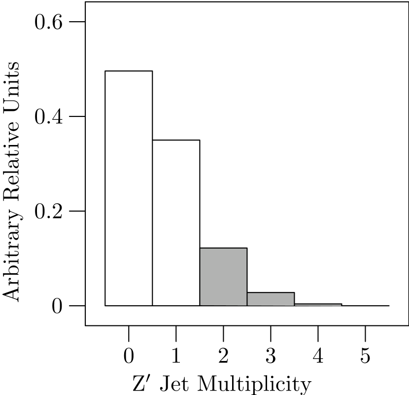
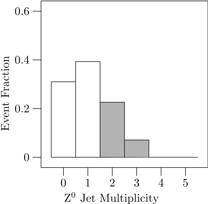
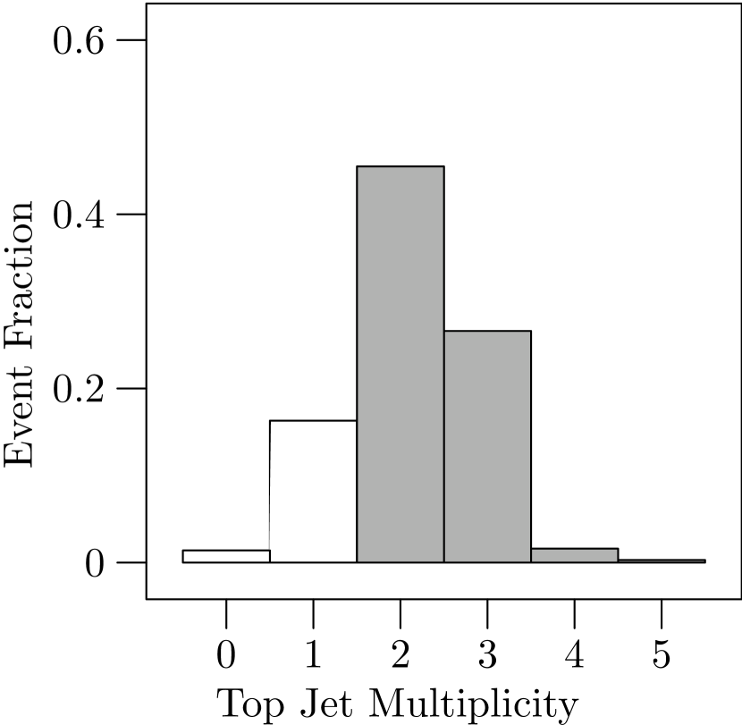
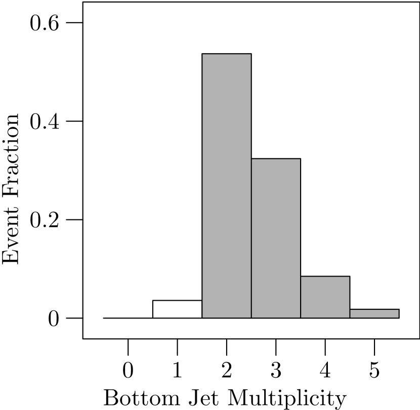
Figure 5: Jet multiplicity for the signal and for each major Standard Model background process following the ${p_{T}^{L}}$ cut. The upper left plot is for the ${\mathrm{Z}^{\prime}}$ signal process, upper center the $\mathrm{Z}^{0}$ background, upper right the $\mathrm{W}$-pair background, and lower left the top background, and the lower right the bottom background. As discussed in the text, all jets of energy exceeding $8\,\mathrm{GeV}$ are included. Each bin is plotted by the fraction of events it contains; the final bin contains all events with $5$ or more jets. Note the qualitative difference between the top and bottom distributions and the other three distributions, which suggests that events with more than one jet be eliminated (these are shaded in gray). The ${\mathrm{Z}^{\prime}}$ plot is for $M_{\mathrm{Z}^{\prime}}=450\,\mathrm{GeV}$ and $s_{\phi}=0.80$.

Note that by rejecting events with jet multiplicity greater than one, we can remove a large majority of the top and bottom backgrounds while minimally impacting the strength of the signal. Comparing the signal-to-background ratio for our model before and after a jet multiplicity cut, we find a significant increase in signal purity, Figure 4.

Next, we apply a topological cut based on the opening angle between the electron and muon, which we will label $\theta_{\mathrm{e}\mathrm{\mu}}$. Given the large mass of the ${\mathrm{Z}^{\prime}}$, we expect it to be produced nearly at rest in the detector, and expect the tau pair to be produced back-to-back and highly boosted. Because of this boost, the electron and muon should be travelling nearly collinearly with their respective parent taus, making them approximately back-to-back with one another in the signal events. The background events would not be expected to have an opening angle distribution that is so highly peaked back-to-back. This is borne out by the Monte Carlo simulation. In Figure 6, we display the distribution of opening angles angles for events which have already passed the ${p_{T}^{L}}$ and jet multiplicity cuts. We choose to eliminate those events with $\cos\theta_{\mathrm{e}\mathrm{\mu}}>-0.5$, that is, those where the electron and muon are not strongly back-to-back. Note that the vast majority of the signal events pass the topological cut, while the background events are more likely to fail it.

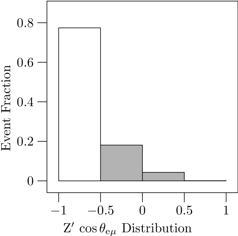
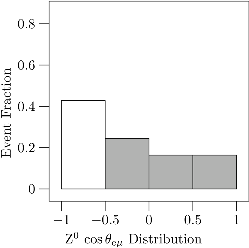
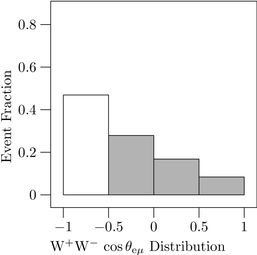
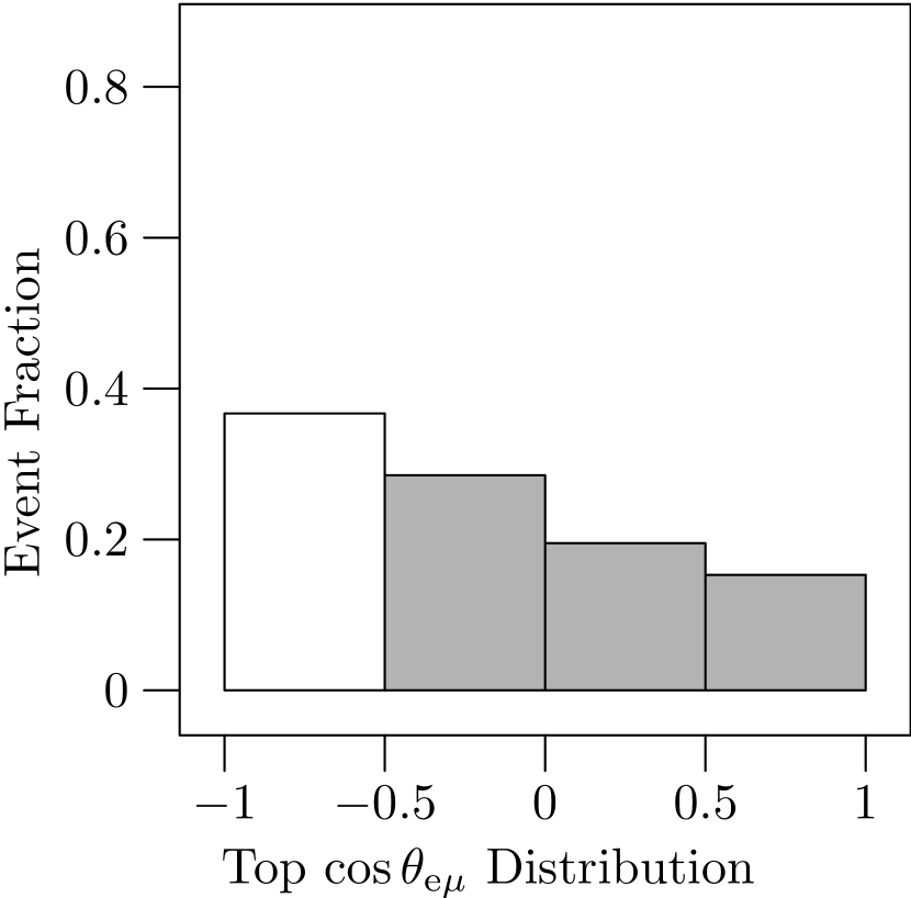
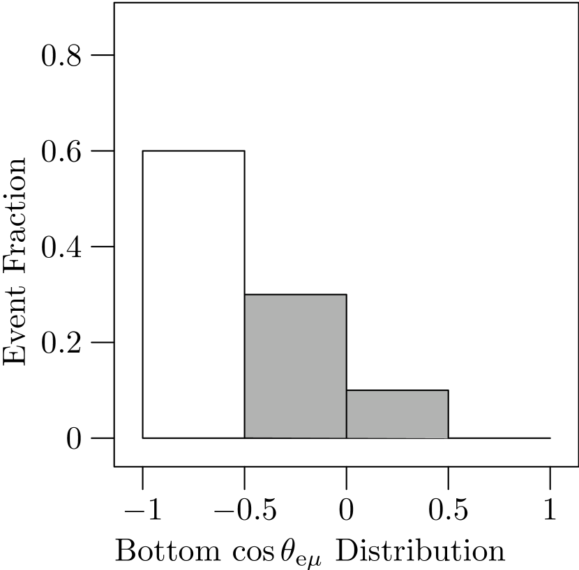
Figure 6: Distribution of opening angles between the electron and muon tracks. We have plotted here the cosines of the opening angle, $\cos\theta_{\mathrm{e}\mathrm{\mu}}$, split into two backward (negative cosine), and two forward (positive cosine) bins, following both the ${p_{T}^{L}}$ and jet multiplicity cuts. The upper left plot is the ${\mathrm{Z}^{\prime}}$ signal process, upper center the $\mathrm{Z}^{0}$ background, upper right the $\mathrm{W}$-pair background, and lower left the top background, and the lower right the bottom background. Note that the vast majority, 80%, of $\mathrm{e}$$\mathrm{\mu}$ pairs from ${\mathrm{Z}^{\prime}}$ signal events are in the “strongly backward” bin (with $\cos\theta<-0.5$), while approximately 40% of $\mathrm{e}$$\mathrm{\mu}$ pairs for all types of background events (except bottom, 60%) are in the “strongly backward” bin. A cut requiring the event to lie in the “strongly backward” bin will eliminate a large group of remaining background events (this group is shaded gray in each figure). The ${\mathrm{Z}^{\prime}}$ plot is for $M_{\mathrm{Z}^{\prime}}=450\,\mathrm{GeV}$ and $s_{\phi}=0.80$.

We have displayed the impact of this topological cut on the signal-to-background ratios for various ${p_{T}^{L}}$ cuts in Figure 4.

At this point, the remaining background is almost purely $\mathrm{W}$-pair. We apply a final topological that that eliminates much of the remaining $\mathrm{W}$-pair background, based on the opening angle between the lowest ${p_{T}}$ lepton and the transverse missing energy in the event, which we label $\theta_{\ell\not E_{T}}$. In order for the event to conserve momentum overall, we would expect the missing transverse energy vector to point along the direction of the softer decay lepton in the $\mathrm{Z}^{0}$ and signal events. Hence, we expect this opening angle to be peaked near $\theta_{\ell\not E_{T}}=0$ for the signal events, while for the other backgrounds, we would not expect this. Based on the opening angle distributions shown in Figure 7, we eliminate events where $\cos\theta_{\ell\not E_{T}}<0.9$, which is particularly effective at eliminating the $\mathrm{W}$-pair background, and particularly ineffective at eliminating signal events.

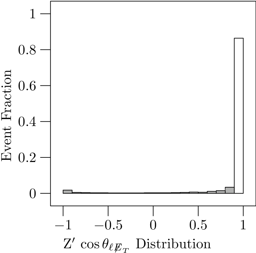
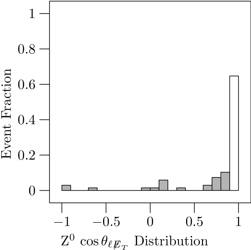
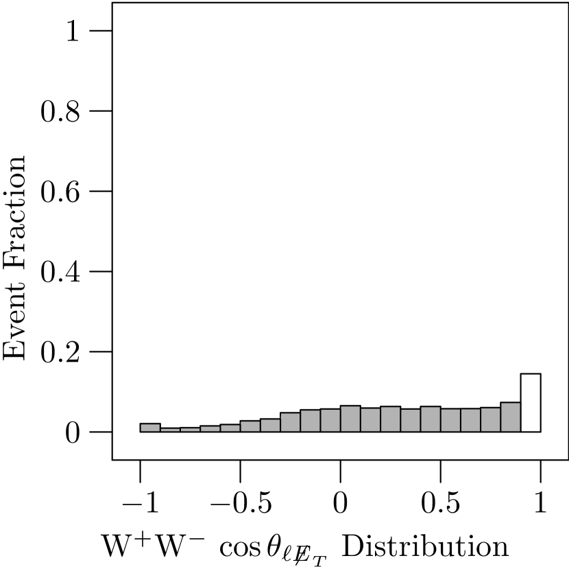
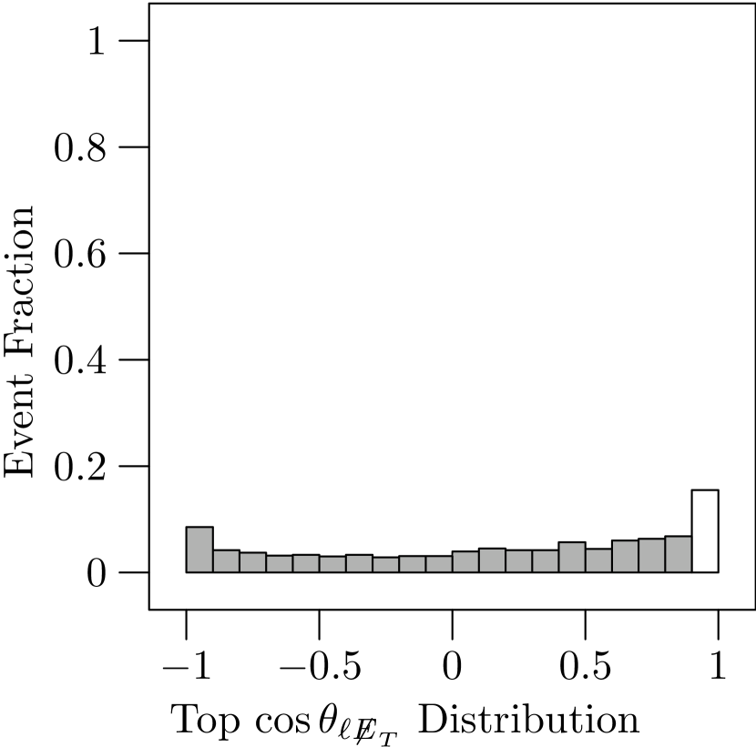
Figure 7: Distribution of $\cos\theta_{\ell\not E_{T}}$, the opening angle between the lowest energy lepton track and the missing energy direction. We have plotted here the fraction of events with given cosine of the opening angle, split into twenty equal bins, following the ${p_{T}^{L}}$, jet multiplicity, and $\theta_{\mathrm{e}\mathrm{\mu}}$ cuts. The upper left plot is the ${\mathrm{Z}^{\prime}}$ signal process, upper right the $\mathrm{Z}^{0}$ background, lower left the $\mathrm{W}$-pair background, and lower right the top background. The bottom background is also reduced by this cut (see Table 1), but the bottom background Monte Carlo sample did not have enough events remaining to produce a smooth distribution at the 20 bin granularity, and so is not plotted here. As discussed in the text, we find the expected qualitative difference between the signal events and the now dominant $\mathrm{W}$-pair background. A cut at small opening angle will preferentially eliminate the $\mathrm{W}$-pair background, and so we choose to require $\cos\theta_{\ell\not E_{T}}>0.90$. The ${\mathrm{Z}^{\prime}}$ plot is for $M_{\mathrm{Z}^{\prime}}=450\,\mathrm{GeV}$ and $s_{\phi}=0.80$.

To summarize the effectiveness of our cuts, we present in Table 1 the fraction of each type of event which survives each cut, along with the expected number of events that survive; overall, roughly 40% of the signal events will survive all four cuts, while substantially less than 1% of all background events will similarly survive.

Event Type	Cuts
	No Cuts		${p_{T}^{L}}$		$n_{\text{jet}}$		$\cos\theta_{\mathrm{e}\mathrm{\mu}}$		$\cos\theta_{\ell\not E_{T}}$
	$\eta$	$\sigma$ (fb)	$\eta$	$\sigma$ (fb)	$\eta$	$\sigma$ (fb)	$\eta$	$\sigma$ (fb)	$\eta$	$\sigma$ (fb)
$\mathrm{SU(2)}$ ${\mathrm{Z}^{\prime}}$ Signal, $M_{\mathrm{Z}^{\prime}}=450\,\mathrm{GeV}$
$s_{\phi}=0.80$	1.00	35.2	0.80	28.0	0.67	23.7	0.58	20.3	0.50	17.5
$\mathrm{U(1)}$ ${\mathrm{Z}^{\prime}}$ Signal, $M_{\mathrm{Z}^{\prime}}=350\,\mathrm{GeV}$
$c_{\phi}=0.80$	1.00	35.7	0.73	26.0	0.62	22.3	0.48	17.2	0.41	14.7
Backgrounds
$\mathrm{Z}^{0}$	1.00	884.3	${<}0.01$	6.7	${<}0.01$	4.7	${<}0.01$	2.0	${<}0.01$	1.3
Top	1.00	92.7	0.65	60.0	0.11	10.6	0.04	3.9	${<}0.01$	0.6
Bottom	1.00	6660.0	0.01	78.0	${<}0.01$	2.8	${<}0.01$	1.7	${<}0.01$	0.8
${\mathrm{W}^{+}}$${\mathrm{W}^{-}}$	1.00	113.4	0.40	45.6	0.34	39.1	0.16	18.4	0.02	2.7
All	1.00	7750.4	0.02	190.3	${<}0.01$	57.2	${<}0.01$	26.0	${<}0.01$	5.4

Table 1: Efficiency of the four event selection cuts. Displayed here are the number of events per inverse femtobarn of luminosity of each type that pass each cut, along with the cumulative efficiency, $\eta$, with which the given cuts retain events. The choice of where to place each of the three cuts is made to maximize the efficiency with which the signal is retained, while simultaneously maximizing the efficiency with which the backgrounds are eliminated and maximizing the overall number of signal events that survive. Overall, roughly 40-50% of the signal events will survive, while less than 1% of the total background will survive for the ${p_{T}^{L}}$, jet, and opening angle cuts discussed in the text.

After performing these cuts on our data, we determined normalized signal and background cross sections from our Monte Carlo data, from which we can obtain luminosity bounds for 90% and 95% exclusion, as well as three and five standard deviation discovery bounds. We will explore first the exclusion reach of the Tevatron, followed by the discovery reach.

Exclusion bounds are obtained by calculating the following Poisson test statistic [27],

$$r(\sigma_{S},\sigma_{B},\mathcal{L})=1-\frac{\sum_{i=0}^{N}\left(S+B\right)^{i}e^{-(S+B)}/i!}{\sum_{i=0}^{N}B^{i}e^{-B}/i!}$$ (4.9)

where $\sigma_{B}$ is the calculated background cross section, $\sigma_{S}$ is the calculated signal cross section, $\mathcal{L}$ is the integrated luminosity, $B=\sigma_{B}\mathcal{L}$ is the expected number of background events, $S=\sigma_{S}\mathcal{L}$ the expected number of signal events, and $N$ is the largest integer smaller than the upper limit on the expected number of background events, that is $N=\lfloor\sigma_{B}\mathcal{L}\rfloor=\lfloor B\rfloor$. For each value of $M_{{\mathrm{Z}^{\prime}}}$ and $s_{\phi}$, taking the calculated signal and background cross sections, we varied the integrated luminosity and determined the statistic $r$. The minimum integrated luminosity required to exclude the model at a given confidence level, ${\mathrm{C}}$, is the luminosity where $r={\mathrm{C}}$. The algorithm determines the ratio of the total probability of $N$ or fewer events occurring in an experiment, for the model of new physics, compared to the probability for standard model physics. At a given confidence level, ${\mathrm{C}}$, the area of overlap between the two probability distributions will be given by $1-{\mathrm{C}}$.

We plot the exclusion limits in Figure 8 for a number of ${\mathrm{Z}^{\prime}}$ masses and a range of mixing parameters, $s_{\phi}$.

Figure 8: Luminosity required to exclude $\mathrm{SU(2)}$ ${\mathrm{Z}^{\prime}}$ bosons of various mass and mixing angles in the extended electroweak scenario of Section 2. We display four pairs of curves, each with a lower dashed curve, the 90% exclusion bound, and an upper solid curve, the 95% exclusion bound. From bottom to top, the curves correspond to ${\mathrm{Z}^{\prime}}$ masses of $600\,\mathrm{GeV}$, $650\,\mathrm{GeV}$, $700\,\mathrm{GeV}$, and $750\,\mathrm{GeV}$. The horizontal lines indicate luminosity targets for Run II, for reference: $2\,\mathrm{fb^{-1}}$, $10\,\mathrm{fb^{-1}}$, and $30\,\mathrm{fb^{-1}}$.

For a ${\mathrm{Z}^{\prime}}$ boson of given mass, the luminosity required for exclusion is lowest when the mixing angle is near $s_{\phi}=0.80$, with an approximately quadratic increase on either side of the minimum. The shape of the exclusion curve reflects the dependence of the ${\mathrm{Z}^{\prime}}$ width on $s_{\phi}$ (cf. Figure 1): narrow ${\mathrm{Z}^{\prime}}$ bosons are easier to detect. With a few inverse femtobarns of integrated luminosity, the ${\mathrm{Z}^{\prime}}\rightarrow\mathrm{\tau}\mathrm{\tau}\to\mathrm{e}\mathrm{\mu}$ channel will begin to explore portions of the model parameter space that are not excluded by the precision electroweak data.

Discovery limits are obtained by applying the following algorithm. For a given integrated luminosity, $\mathcal{L}$, we expect to observe $B=\sigma_{B}\mathcal{L}$ background events, and $S=\sigma_{S}\mathcal{L}$ signal events, for a total of $S+B$ expected events. We calculate the Poisson probability, $P(\mu,x)$, that an expected background of $\mu=B$ events could fluctuate to give us a false signal of $x=S+B$ events total, that is $P(B,S+B)$. If the probability of such a fluctuation is smaller than a given confidence level, we are justified in declaring discovery of a new phenomenon at that level. We choose to determine the luminosity, $\mathcal{L}$, for three gaussian standard deviation discovery (which we denote as $3\sigma$), where $P(B,S+B)_{3\sigma}\leq 1.35\times 10^{-3}$, and for $5\sigma$, where $P(B,S+B)\leq 2.7\times 10^{-7}$. We plot discovery bounds for a number of ${\mathrm{Z}^{\prime}}$ masses and a range of mixing parameter, $s_{\phi}$, in Figure 9

Figure 9: Luminosity required to discover $\mathrm{SU(2)}$ ${\mathrm{Z}^{\prime}}$ bosons of various masses and mixing angles in the extended electroweak scenario of Section 2. We display two types of curves. Dashed curves are $3\sigma$ discovery curves for a fixed mass, while solid curves are $5\sigma$ discovery curves. From bottom to top, $3\sigma$ curves are displayed for ${\mathrm{Z}^{\prime}}$ masses of 550 GeV, 600 GeV, 650 GeV, and 700 GeV. From bottom to top, $5\sigma$ curves are displayed for ${\mathrm{Z}^{\prime}}$ masses of 550 GeV, 600 GeV, and 650 GeV. The horizontal lines indicate luminosity targets for Run II, for reference: $2\,\mathrm{fb^{-1}}$, $10\,\mathrm{fb^{-1}}$, and $30\,\mathrm{fb^{-1}}$.

As expected from the previously determined exclusion bounds, for a ${\mathrm{Z}^{\prime}}$ boson of a given mass, the luminosity for discovery is lowest when the mixing angle is near $s_{\phi}=0.80$. As with exclusion, only a few inverse femtobarns of integrated luminosity will be required to discover a ${\mathrm{Z}^{\prime}}$ boson with mass just above the current exclusion bounds.

By studying the $\mathrm{e}$$\mathrm{\mu}$ invariant mass distribution ($M_{\mathrm{e}\mathrm{\mu}}=|p_{\mathrm{\mu}}+p_{\mathrm{e}}|$) it may be possible to detect the presence of a ${\mathrm{Z}^{\prime}}$ boson and to determine its mass. As shown in Figure 10,

Figure 10: Electron-muon invariant mass ($M_{\mathrm{e}\mathrm{\mu}}=|p_{\mathrm{e}}+p_{\mathrm{\mu}}|$) distribution for signal plus background events surviving all cuts. For comparison, the distribution for all background events is shaded. The presence of a heavy ${\mathrm{Z}^{\prime}}$ boson clearly alters the distribution of events, toward higher invariant mass. Variation of the mixing angle for a fixed mass ${\mathrm{Z}^{\prime}}$ impacts the event rate of the distributions, but roughly speaking, not the shape or location of the peak. The distributions displayed here are for $M_{{\mathrm{Z}^{\prime}}}=450\,\mathrm{GeV}$ and $s_{\phi}=0.60$, and for $M_{{\mathrm{Z}^{\prime}}}=450\,\mathrm{GeV}$ and $s_{\phi}=0.80$.

the invariant mass distribution of the background events which pass all of our cuts peak at around $100\,\mathrm{GeV}$. The centroid of the distribution of signal events is shifted toward higher invariant mass, with the amount of the shift depending on the value of $M_{\mathrm{Z}^{\prime}}$, but almost independent of $s_{\phi}$, Figure 11.

Figure 11: We plot the centroids of the $\mathrm{e}$$\mathrm{\mu}$ invariant mass distributions, $M_{\mathrm{e}\mathrm{\mu}}$. The plot on the left displays the centroids of the signal distributions as a function of mass and mixing angle. Note that the centroids are nearly independent of the mixing angle. We do not, however, measure the signal in isolation, but in the presence of backgrounds. The plot on the right displays the centroids of the combined signal and background distributions. Here, the separation of the model parameters based on the data is less straightforward, although clearly differentiated from the background distribution alone. The solid curves, from bottom to top in the left plot, correspond to ${\mathrm{Z}^{\prime}}$ masses of 450 GeV, 550 GeV, 650 GeV, and 750 GeV; the dotted line at the bottom is the centroid of the background by itself. The signal plus background distributions in the right plot all essentially overlap, but are separated from the background distribution. The dotted line at the bottom is the centroid of the background by itself. The solid curves, from bottom to top, correspond to ${\mathrm{Z}^{\prime}}$ masses of 750 GeV, 450 GeV, 650 GeV, and 550 GeV.

However, as the background rate is independent of the mixing angle while the signal rate is not, the centroid of the background plus signal distribution is not sufficient on its own to determine the mass. With a sufficiently high data rate, available at the LHC for example, it may be possible to choose more aggressive cuts that would lessen the dependence of the centroid on the background; it may alternatively be possible to perform a background subtraction on the invariant mass distribution, although this approach is more difficult to perform with confidence. With enough data, then, it should be possible to determine $M_{\mathrm{Z}^{\prime}}$ from the measured invariant mass distribution $M_{\mathrm{e}\mathrm{\mu}}$.

Determining the value of $s_{\phi}$ will be more challenging. As indicated by the shape of the exclusion curves in Figure 8, the relationship between event-rate and $s_{\phi}$ is double-valued: a given event rate corresponds to two values of $s_{\phi}$, one above and one below $s_{\phi}=0.80$ (approx.). Finding evidence of ${\mathrm{Z}^{\prime}}\rightarrow\mathrm{e}^{+}\mathrm{e}^{-},\ \mathrm{\mu}^{+}\mathrm{\mu}^{-}$ may allow one to differentiate between the two possible values of $s_{\phi}$ due to the different forms of the couplings: the first or second generation lepton couplings vary as $c_{\phi}/s_{\phi}$, while to the third generation couplings vary as $s_{\phi}/c_{\phi}$.

5 ${\mathrm{Z}^{\prime}}$ Bosons from Extended Hypercharge Interactions

Models with an extended hypercharge gauge group can also produce heavy ${\mathrm{Z}^{\prime}}$ bosons that couple more strongly to the third generation than to the lighter generations [3, 8, 28, 10]. In these theories, the electroweak gauge group is

$$\mathrm{SU(2)}_{W}\times\mathrm{U(1)}_{h}\times\mathrm{U(1)}_{\ell}$$ (5.1)

where third-generation fermions couple to $\mathrm{U(1)}_{h}$ with standard hypercharge values and the other fermions are carry standard hypercharges under $\mathrm{U(1)}_{\ell}$. At a scale above the weak scale, the two hypercharge groups break to their diagonal subgroup, identified as $\mathrm{U(1)}_{Y}$. As a result, a ${\mathrm{Z}^{\prime}}$ boson that is a linear combination of the original two hypercharge bosons becomes massive. This heavy ${\mathrm{Z}^{\prime}}$ boson couples to fermions as

$$-i\frac{e}{\cos\theta}\left(\frac{s_{\chi}}{c_{\chi}}Y_{\ell}-\frac{c_{\chi}}{s_{\chi}}Y_{h}\right)$$ (5.2)

where $\chi$ is the mixing angle between the two original hypercharge sectors

$$\cot{\chi}=\left(\frac{g_{h}}{g_{\ell}}\right)^{2}\ .$$ (5.3)

Comparing Equation 5.2 with the covariant derivative for the ${\mathrm{Z}^{\prime}}$ boson from an extended weak group, Equation 2.15, we find three key differences. Two are physically relevant: the overall coupling is of hypercharge rather than weak strength, and the ${\mathrm{Z}^{\prime}}$ couples to both left-handed and right-handed fermions at leading order. One is a matter of convention: mixing angle $\chi$ is equivalent to $\pi/2-\phi$.

At energies well below the mass of the ${\mathrm{Z}^{\prime}}$ boson, its exchange in the process $\mathrm{e}^{+}\mathrm{e}^{-}\rightarrow f\overline{f}$ where $f$ is a $\mathrm{\tau}$ lepton or $\mathrm{b}$ quark may be approximated by the contact interaction

$$\mathcal{L}_{\mathrm{NC}}\supset\frac{e^{2}}{\cos^{2}\theta M^{2}_{{\mathrm{Z}^{\prime}}}}\left(\frac{s_{\chi}}{c_{\chi}}\big{[}\overline{\mathrm{e}}\gamma_{\mu}Y_{\ell}\mathrm{e}\big{]}\right)\left(\frac{c_{\chi}}{s_{\chi}}\big{[}\overline{f}\gamma^{\mu}Y_{h}f\big{]}\right)$$ (5.4)

Comparing this with the contact interactions studied by LEP (see Section 3.1), we find that the LEP data sets its strongest limit through the process $\mathrm{e}^{+}_{R}\mathrm{e}^{-}_{R}\rightarrow\mathrm{\tau}^{+}_{R}\mathrm{\tau}^{-}_{R}$ [20, 21],

$$\Lambda(f=\mathrm{\tau},\ \eta_{RR}=+1)>\begin{cases}3.7\,\mathrm{TeV}&\text{ALEPH}\\ 3.7\,\mathrm{TeV}&\text{OPAL}\ ,\end{cases}$$ (5.5)

which gives a limit on the ${\mathrm{Z}^{\prime}}$ mass of

$$M_{{\mathrm{Z}^{\prime}}}=\Lambda\sqrt{\frac{\alpha_{\mathrm{em}}}{\cos^{2}\theta}}>370\,\mathrm{GeV}\ .$$ (5.6)

This is stronger than the previous limits from precision electroweak data [11].

We have also used the techniques described in Section 4 to analyze the process $\mathrm{p}\overline{\mathrm{p}}\rightarrow{\mathrm{Z}^{\prime}}\rightarrow\mathrm{\tau}\mathrm{\tau}\rightarrow\mathrm{e}\mathrm{\mu}$ for a $\mathrm{U(1)}$ ${\mathrm{Z}^{\prime}}$ boson. Due to the similar form of couplings of the ${\mathrm{Z}^{\prime}}$ bosons to fermions, we obtain results for exclusion and discovery bounds that can be expected from the Tevatron that depend on mixing angle in a similar fashion. We display exclusion bounds in Figure 12

Figure 12: Luminosity required to exclude $\mathrm{U(1)}$ ${\mathrm{Z}^{\prime}}$ bosons of various mass and mixing angles in the extended hypercharge scenario of Section 5. We display four pairs of curves, each with a lower dashed curve, the 90% exclusion bound, and an upper solid curve, the 95% exclusion bound. From bottom to top, the curves correspond to ${\mathrm{Z}^{\prime}}$ masses of $500\,\mathrm{GeV}$, $550\,\mathrm{GeV}$, $600\,\mathrm{GeV}$, and $650\,\mathrm{GeV}$. The horizontal lines correspond to the luminosity targets for Run II, displayed for ease of reference: $2\,\mathrm{fb^{-1}}$, $10\,\mathrm{fb^{-1}}$, and $30\,\mathrm{fb^{-1}}$.

and discovery bounds in Figure 13.

Figure 13: Luminosity required to discover $\mathrm{U(1)}$ ${\mathrm{Z}^{\prime}}$ bosons of various masses and mixing angles in the extended hypercharge scenario of Section 5. We display two types of curves. Dashed curves are $3\sigma$ discovery curves for a fixed mass, while solid curves are $5\sigma$ discovery curves. From bottom to top, $3\sigma$ curves are displayed for ${\mathrm{Z}^{\prime}}$ masses of 450 GeV, 500 GeV, 550 GeV, and 600 GeV. From bottom to top, $5\sigma$ curves are displayed for ${\mathrm{Z}^{\prime}}$ masses of 450 GeV, 500 GeV, and 550 GeV. The horizontal lines indicate luminosity targets for Run II, for reference: $2\,\mathrm{fb^{-1}}$, $10\,\mathrm{fb^{-1}}$, and $30\,\mathrm{fb^{-1}}$.

The luminosity required to exclude or discover a $\mathrm{U(1)}$ ${\mathrm{Z}^{\prime}}$ boson is a bit greater than for an $\mathrm{SU(2)}$ ${\mathrm{Z}^{\prime}}$ boson of the same mass. This difference reflects the fact that the $\mathrm{U(1)}$ boson’s coupling to fermions is of hypercharge rather than weak strength.

6 Future Searches

Detecting even relatively light ${\mathrm{Z}^{\prime}}$ bosons that couple preferentially to third-generation fermions is clearly a challenge for Tevatron and LEP experiments. Even in the $p\bar{p}\rightarrow{\mathrm{Z}^{\prime}}\rightarrow\mathrm{\tau}\mathrm{\tau}\rightarrow\mathrm{e}\mathrm{\mu}$ process where the signal-to-background ratio can be made quite large, the absolute number of signal events is kept low by the size of the ${\mathrm{Z}^{\prime}}$ boson’s coupling to the light fermions from which it is produced. In the long term, the LHC’s higher center-of-mass energy will allow its experiments to search for these ${\mathrm{Z}^{\prime}}$ bosons without being hampered by low signal event rates. In the meantime, we suggest that a few additional search channels may prove useful.

Obviously, the reach in $\mathrm{\tau}^{+}$$\mathrm{\tau}^{-}$ final states will be extended beyond that shown in this analysis if use can be made of one or more hadronic tau decays . The single-prong decays of the tau, which constitutes about 85% of all decays, may have sufficiently small background since QCD should rarely produce isolated, high-${p_{T}}$ tracks. It will be difficult to use these final states to search for ${\mathrm{Z}^{\prime}}$ bosons: it is extremely hard, in the hadronic environment, to trigger on jets, and flavor tagging with high precision is an unresolved problem. Nonetheless, since the branching ratio of $\mathrm{\tau}$ to hadrons ($\mathrm{BR}(\mathrm{\tau}\rightarrow\text{hadrons})\approx 65\%$) is higher than to leptons ($\mathrm{BR}(\mathrm{\tau}\rightarrow\text{leptons})\approx 35\%$) [30], even modest jet trigger and flavor tagging efficiencies could prove extremely valuable in searches or measurement of parameters. The ability to use these additional channels with their higher event rates should yield significantly improved mass limits for a given integrated luminosity.

In the semi-leptonic decay scenario, where we have $\mathrm{\tau}^{+}\mathrm{\tau}^{-}\rightarrow\text{jet}+\ell$, the event trigger could be a high-${p_{T}}$ electron or muon with, for example, ${p_{T}}>15\,\mathrm{GeV}$. In offline processing, one would then reconstruct the jets, and attempt to perform flavor tagging. If the corrected $\mathrm{\tau}$ tagging efficiency can be raised to approximately 15%, then the semi-leptonic events will provide the same event rate for analysis as the fully leptonic events previously considered. Further study of these channels are clearly warranted.

${\mathrm{Z}^{\prime}}$ bosons arising from extended weak interactions will also be accompanied by ${\mathrm{W}^{\prime}}$ bosons of very similar mass (to leading order, $M_{\mathrm{Z}^{\prime}}=M_{\mathrm{W}^{\prime}}$). These bosons could be searched for in the process $\mathrm{p}\overline{\mathrm{p}}\rightarrow{\mathrm{W}^{\prime}}\rightarrow\mathrm{\tau}\mathrm{\nu}_{\mathrm{\tau}}$. Standard model backgrounds would include $\mathrm{p}\overline{\mathrm{p}}\rightarrow W\rightarrow\ell\mathrm{\nu}_{\ell}$ and $\mathrm{p}\overline{\mathrm{p}}\rightarrow\mathrm{W}\mathrm{Z}^{0}\rightarrow\ell\mathrm{\nu}_{\ell}\mathrm{\nu}\mathrm{\nu}$, both of which should have softer lepton spectra, as well as $\mathrm{p}\overline{\mathrm{p}}\rightarrow\mathrm{Z}^{0}+\text{jet}\rightarrow\mathrm{\nu}\mathrm{\nu}+\text{fake lepton}$, where the jet is misidentified.

The methods of analysis pursued in Section 4 could productively be applied to models with scalars that have large branching ratios to tau pairs. While a heavy Standard Model Higgs boson does not have a high enough branching ratio for these analyses to provide useful limits, a pseudoscalar Higgs with large branching ratio would be an interesting candidate for study.

7 Conclusions

We have discussed two methods of searching for ${\mathrm{Z}^{\prime}}$ bosons that couple primarily to third generation fermions. Bounds on the scale of quark-lepton compositeness derived from data taken at LEP and the Tevatron now imply that ${\mathrm{Z}^{\prime}}$ bosons derived from extended $\mathrm{SU(2)}_{h}\times\mathrm{SU(2)}_{\ell}$ or $\mathrm{U(1)}_{h}\times\mathrm{U(1)}_{\ell}$ interactions must have a mass greater than about $375\,\mathrm{GeV}$. The reach of these limits will improve as additional data is taken. As the Tevatron Run II begins, it will become possible to search for ${\mathrm{Z}^{\prime}}$ bosons using the process $p\overline{p}\to{\mathrm{Z}^{\prime}}\to\mathrm{\tau}\mathrm{\tau}\to\mathrm{e}\mathrm{\mu}\mathrm{X}$. We have shown that a combination of cuts based on lepton transverse momenta, jet multiplicity, and event topology, can overcome the standard model backgrounds. With $30\,\mathrm{fb^{-1}}$ of data, the Run II experiments will be able to exclude ${\mathrm{Z}^{\prime}}$ bosons with masses up to $750\,\mathrm{GeV}$. Were a ${\mathrm{Z}^{\prime}}$ boson, instead, discovered, the shape of the $\mathrm{e}$$\mathrm{\mu}$ invariant mass distribution and the relative branching fractions to taus and to muons could reveal the ${\mathrm{Z}^{\prime}}$ mass and coupling strength.

Acknowledgments

The authors thank C. Hoelbling, F. Paige, and M. Popovic for useful conversations, and K. Lane and P. Kalyniak for comments on the manuscript. E.H.S. acknowledges the support of the NSF Faculty Early Career Development (CAREER) program and the DOE Outstanding Junior Investigator program. M.N. acknowledges the support of the NSF Professional Opportunities for Women in Research and Education (POWRE) program. This work was supported in part by the National Science Foundation under grants PHY-9501249 and PHY-9870552, by the Department of Energy under grant DE-FG02-91ER40676, and by the Davis Institute for High Energy Physics.

References

• [1] C.T. Hill, Phys. Lett.  B 266 419 (1991)
• [2] R.S. Chivukula, E.H. Simmons, J. Terning, Phys. Lett.  B 331, 383 (1994), hep-ph/9404209; R.S. Chivukula, E.H. Simmons, J. Terning, Phys. Rev.  D 53, 5258 (1996), hep-ph/9506427.
• [3] C.T. Hill, Phys. Lett.  B 345, 483 (1995), hep-ph/9411426.
• [4] R.S. Chivukula, A.G. Cohen and E.H. Simmons, Phys. Lett.  B 380, 92 (1996), hep-ph/9603311.
• [5] D.J. Muller and S. Nandi, Phys. Lett.  B 383, 354 (1996), hep-ph/9602390; E. Malkawi, T. Tait, and C.P. Yuan, Phys. Lett.  B 385, 304 (1996), hep-ph/9603349; D.J. Muller and S. Nandi, Nucl. Phys. Proc. Suppl. 52A, 192 (1997), hep-ph/9607328; D.J. Muller and S. Nandi, Proceedings, ICHEP 96, Warsaw Poland, 25-31 July 1996 (ICHEP 96:1409), hep-ph/9610404.
• [6] E.H. Simmons, Phys. Rev.  D 55, 5494 (1997), hep-ph/9612402.
• [7] H.J. He, T. Tait, and C.P. Yuan, Phys. Rev.  D 62 (2000) 011702, hep-ph/9911266.
• [8] K. Lane and E. Eichten, Phys. Lett.  B 352, 382 (1995), hep-ph/9503433; K.D. Lane, Phys. Rev.  D 54, 2204 (1996), hep-ph/9602221.
• [9] K.D. Lane, Phys. Lett.  B 433, 96 (1998), hep-ph/9805254.
• [10] M.B. Popovic and E.H. Simmons, Phys. Rev.  D 58, 095007 (1998) hep-ph/9806287.
• [11] R.S. Chivukula and J. Terning, Phys. Lett.  B 385, 209 (1996), hep-ph/9606233.
• [12] M. Cvetic and P. Langacker, “${\mathrm{Z}^{\prime}}$ physics and supersymmetry,” hep-ph/9707451.
• [13] G. Cleaver et al., Phys. Rev.  D 59, 055005 (1999), hep-ph/9807479 and references therein.
• [14] J. Erler and P. Langacker, Phys. Rev. Lett.  84, 212 (2000), hep-ph/9910315.
• [15] M. Cvetiĉ and S. Godfrey, in Electroweak Symmetry Breaking and Beyond the Standard Model, Eds. T. Barklow et al., hep-ph/9504216; S. Godfrey Phys. Rev.  D 51, 1402 (1995); S. Capstick and S. Godfrey, Phys. Rev.  D 37, 2466 (1988).
• [16] CDF Collaboration. F. Abe et al., Phys. Rev. Lett.  82, 2038 (1999), hep-ex/9809022.
• [17] CDF Collaboration. T. Affolder, et al., Submitted to Phys. Rev. Lett.  (2000). hep-ex/0003005.
• [18] E. Malkawi and C. P. Yuan, Phys. Rev.  D 61, 015007 (2000), hep-ph/9906215; P. Langacker and M. Plumacher, Phys. Rev.  D 62, 013006 (2000), hep-ph/0001204.
• [19] H. Georgi, E.E. Jenkins, and E.H. Simmons, Phys. Rev. Lett.  62, 2789 (1989) and Erratum Phys. Rev. Lett.  63, 1540 (1989) and Nucl. Phys.  B 331, 541 (1990).
• [20] ALEPH Collaboration, R. Barate et al., Eur. Phys. J. C 12, 183 (2000). DOI 10.1007/s100529900223.
• [21] OPAL Collaboration, G. Abbiendi et al., Eur. Phys. J. C 6, 1 (1999). DOI 10.1007/s100529801027
• [22] E. Eichten, K. Lane, and M.E. Peskin, Phys. Rev. Lett.  50 (1983) 811.
• [23] CDF Collaboration, F. Abe et al., Phys. Rev. Lett.  79, 2198 (1997), FERMILAB-PUB-97-171-E.
• [24] DØ Collaboration, B. Abbot et al., Phys. Rev. Lett.  82, 4769 (1999), hep-ex/9812010.
• [25] D. Amidei and R. Brock, eds. Future Electroweak Physics at the Fermilab Tevatron: Report of the TeV 2000 Study Group, FERMILAB-PUB-96-082 (1996).
• [26] T. Sjöstrand, Comp. Phys. Comm. 82, 74 (1994).
• [27] J. Conway and K. Maeshima, CDF/PUB/EXOTIC/PUBLIC-4476, (1998); J. Conway, H. Haber, J. Hobbs, H. Prosper, Statistical Conventions and Method for Combining Channels for the Tevatron Run 2 SUSY/Higgs Workshop, Higgs Working Group, http://fnth37.fnal.gov/higgs/conv5.ps.
• [28] G. Buchalla et al., Phys. Rev.  D 53, 5185 (1996), hep-ph/9510376.
• [29] E. Ma and D. P. Roy, Phys. Rev.  D 58, 095005 (1998), hep-ph/9806210.
• [30] Particle Data Group: C. Caso et al., Eur. Phys. J. C C3, 227 (1998), http://pdg.lbl.gov.