TPR-00-10 hep-ph/0007279

Higher Twist Distribution Amplitudes of the Nucleon in QCD

V. Braun, R. J. Fries, N. Mahnke, and E. Stein,

Institut für Theoretische Physik , Universität Regensburg, D-93040 Regensburg, Germany

Abstract
We present the first systematic study of higher-twist light-cone distribution amplitudes of the nucleon in QCD. We find that the valence three-quark state is described at small transverse separations by eight independent distribution amplitudes. One of them is leading twist-3, three distributions are twist-4 and twist-5, respectively, and one is twist-6. A complete set of distribution amplitudes is constructed, which satisfies equations of motion and constraints that follow from conformal expansion. Nonperturbative input parameters are estimated from QCD sum rules.
Submitted to Nuclear Physics B

PACS numbers:

Keywords: QCD, Nucleon, Power Corrections, Distribution Amplitudes

1 Introduction

Hard exclusive processes are coming to the forefront of high energy nuclear and particle physics. This is already visible at TJNAF, COMPASS, HERMES that go for more and more exclusive channels, and it makes the core of the ELFE proposal. One main reason for that is the growing understanding that exclusive reactions provide unmatched opportunities to study the hadron structure, as demonstrated by recent interest to deeply virtual Compton scattering (DVCS) and hard diffractive meson production. All future plans also call for very high luminosity and would therefore be perfectly suited for the investigation of exclusive and semi-exclusive reactions with and without polarization.

The classical theoretical framework for the calculation of hard exclusive processes in QCD was developed in [1, 2], see [3, 4, 5] for a review. This approach introduces a concept of hadron distribution amplitudes as fundamental nonperturbative functions describing the hadron structure in rare parton configurations with a minimum number of Fock constituents (and at small transverse separations). The distribution amplitudes are equally important and to a large extent complementary to conventional parton distributions which correspond to one-particle probability distributions for the parton momentum fraction in an average configuration. The recent data from CLEO [6] and E791 [7] provided, for the first time, quantitative information on the pion distribution amplitude.

For a theorist, the main challenge is to make the QCD description of hard exclusive reactions fully quantitative. Although the leading-twist QCD factorization approach correctly reproduces the power dependence of exclusive amplitudes on the large momentum, there exist many indications that soft end-point and higher-twist corrections might dominate over the naive QCD prediction over the range of accessible values of $Q^{2}$. For mesons, the study of preasymptotic corrections to exclusive reactions has been pursued intensively and in different directions. In particular, meson distribution amplitudes of higher twist have been studied in detail in [3, 8, 9]. For baryons, the corresponding task is more complicated and received less attention in the past. Soft end-point contributions to several hard exclusive reactions involving nucleons have been estimated using various models and were found to be large [10]. To the best of our knowledge, hard higher-twist corrections and nucleon mass corrections have never been addressed in the literature. In this paper we present the first systematic study of nucleon distribution amplitudes of higher twist.

The notion of higher twist contributions to the distribution amplitudes comprises a broad spectrum of effects of different physical origin: First, contributions of “bad” components in the wave function and in particular of components with “wrong” spin projection; second, contributions of transverse motion of quarks (antiquarks) in the leading twist components; third, contributions of higher Fock states with additional gluons and/or quark-antiquark pairs. Finally, one can speak of hadron mass effects, similar to target mass corrections in deep inelastic scattering. The relative significance of these corrections depends on the hadron state in question and the particular hard process. There exists an important conceptual difference between mesons and baryons. For mesons, all effects due to “bad” components in the quark-antiquark wave functions can be rewritten in terms of higher Fock state components thanks to the QCD equations of motion. Since quark-antiquark-gluon matrix elements between the vacuum and the meson state are numerically small (see [8, 9] for the existing estimates), contributions of “bad” components in two-particle wave functions are small as well, and to a large extent dominated by meson mass corrections [8, 9]. For baryons, on the contrary, QCD equations of motion are not sufficient to eliminate the higher-twist three-quark states in favor of the components with extra gluons, so that the former present genuine new degrees of freedom. Moreover, vacuum-to-baryon matrix elements of higher-twist three-quark operators are large, comparable to the ones of leading twist. One may expect, therefore, that higher-twist effects in baryon wave functions are dominated by “bad” components of three-quark states rather than extra gluons. A systematic study of such states as well as taking into account nucleon mass corrections presents the subject of this work.

We find that a generic three-quark matrix element on the light-cone can be parametrized in terms of eight independent distribution amplitudes. In particular, there exists one amplitude of leading twist-three that is familiar from earlier studies [2, 11], three distribution amplitudes of twist-four and twist-five, respectively, and one distribution amplitude of twist-six. Following the approach of [8, 9], we further expand all distribution amplitudes in contributions of operators with increasing conformal spin. The conformal expansion corresponds, physically, to the separation of longitudinal and transverse degrees of freedom, and the coefficients of this expansion present the relevant nonperturbative parameters. We find that the higher-twist distribution amplitudes with the lowest conformal spin (asymptotic wave functions) involve two nonperturbative matrix elements that are well known from the QCD sum rule studies of the nucleon [12, 13, 14]. The leading corrections to the asymptotic wave functions involve three more parameters (for all twists) that we estimate in this work.

The outline of the paper is as follows. The general classification of twist-three distribution amplitudes is worked out in Section 2. One starts with 24 invariant functions in a general decomposition of a three quark light-cone operator. By isospin symmetry the number of independent amplitudes is reduced to eight amplitudes that determine the three-quark proton state completely. A convenient representation of these independent amplitudes is derived in terms of chiral fields.

Section 3 is devoted to the conformal expansion. We identify the nonperturbative parameters that describe the higher-twist distribution amplitudes up to next-to-leading order in the conformal expansion and work out the relations between them, as given by isospin constraints and equations of motion.

In Section 4 we present particular models for the higher-twist distributions based on QCD sum rules and summarize.

Our work encloses a number of appendices. Appendix A gives the Fierz transformation rules used to derive the isospin relations. Appendix B summarizes the determination of nonperturbative parameters in the QCD sum rule approach. Appendix C contains a “handbook” of nucleon distribution amplitudes where we collect all expressions needed in practical calculations.

2 General classification

2.1 Lorentz structure

The notion of hadron distribution amplitudes in general refers to hadron-to-vacuum matrix elements of nonlocal operators built of quark and gluon fields at light-like separations. In this paper we will deal with the three-quark matrix element

$$\left\langle 0\right|\varepsilon^{ijk}u_{\alpha}^{i^{\prime}}(a_{1}z)\left[a_{1}z,a_{0}z\right]_{i^{\prime},i}u_{\beta}^{j^{\prime}}(a_{2}z)\left[a_{2}z,a_{0}z\right]_{j^{\prime},j}d_{\gamma}^{k^{\prime}}(a_{3}z)\left[a_{3}z,a_{0}z\right]_{k^{\prime},k}\left|P(P,\lambda)\right\rangle$$ (2.1)

where $\left|P(P,\lambda)\right\rangle$ denotes the proton state with momentum $P$, $P^{2}=M^{2}$ and helicity $\lambda$. $u,d$ are the quark-field operators. The Greek letters $\alpha,\beta,\gamma$ stand for Dirac indices, the Latin letters $i,j,k$ refer to color. $z$ is an arbitrary light-like vector, $z^{2}=0$, the $a_{i}$ are real numbers. The gauge-factors $\left[x,y\right]$ are defined as

$$\left[x,y\right]={\rm P}\exp\left[ig\int_{0}^{1}\!{\rm d}t\,(x-y)_{\mu}A^{\mu}(tx+(1-t)y)\right]\,$$ (2.2)

and render the matrix element in (2.1) gauge-invariant. To simplify the notation we will not write the gauge-factors explicitely in what follows but imply that they are always present.

Taking into account Lorentz covariance, spin and parity of the nucleon, the most general decomposition of the matrix element in Eq. (2.1) involves 24 invariant functions:

$$4\left\langle 0\right|\varepsilon^{ijk}u_{\alpha}^{i}(a_{1}z)u_{\beta}^{j}(a_{2}z)d_{\gamma}^{k}(a_{3}z)\left|P\right\rangle=$$ (2.3)

$$= {\cal S}_{1}MC_{\alpha\beta}\left(\gamma_{5}N\right)_{\gamma}+{\cal S}_{2}M^{2}C_{\alpha\beta}\left(\!\not\!{z}\gamma_{5}N\right)_{\gamma}+{\cal P}_{1}M\left(\gamma_{5}C\right)_{\alpha\beta}N_{\gamma}+{\cal P}_{2}M^{2}\left(\gamma_{5}C\right)_{\alpha\beta}\left(\!\not\!{z}N\right)_{\gamma}$$

$$+{\cal V}_{1}\left(\!\not\!{P}C\right)_{\alpha\beta}\left(\gamma_{5}N\right)_{\gamma}+{\cal V}_{2}M\left(\!\not\!{P}C\right)_{\alpha\beta}\left(\!\not\!{z}\gamma_{5}N\right)_{\gamma}+{\cal V}_{3}M\left(\gamma_{\mu}C\right)_{\alpha\beta}\left(\gamma^{\mu}\gamma_{5}N\right)_{\gamma}$$

$$+{\cal V}_{4}M^{2}\left(\!\not\!{z}C\right)_{\alpha\beta}\left(\gamma_{5}N\right)_{\gamma}+{\cal V}_{5}M^{2}\left(\gamma_{\mu}C\right)_{\alpha\beta}\left(i\sigma^{\mu\nu}z_{\nu}\gamma_{5}N\right)_{\gamma}+{\cal V}_{6}M^{3}\left(\!\not\!{z}C\right)_{\alpha\beta}\left(\!\not\!{z}\gamma_{5}N\right)_{\gamma}$$

$$+{\cal A}_{1}\left(\!\not\!{P}\gamma_{5}C\right)_{\alpha\beta}N_{\gamma}+{\cal A}_{2}M\left(\!\not\!{P}\gamma_{5}C\right)_{\alpha\beta}\left(\!\not\!{z}N\right)_{\gamma}+{\cal A}_{3}M\left(\gamma_{\mu}\gamma_{5}C\right)_{\alpha\beta}\left(\gamma^{\mu}N\right)_{\gamma}$$

$$+{\cal A}_{4}M^{2}\left(\!\not\!{z}\gamma_{5}C\right)_{\alpha\beta}N_{\gamma}+{\cal A}_{5}M^{2}\left(\gamma_{\mu}\gamma_{5}C\right)_{\alpha\beta}\left(i\sigma^{\mu\nu}z_{\nu}N\right)_{\gamma}+{\cal A}_{6}M^{3}\left(\!\not\!{z}\gamma_{5}C\right)_{\alpha\beta}\left(\!\not\!{z}N\right)_{\gamma}$$

$$+{\cal T}_{1}\left(P^{\nu}i\sigma_{\mu\nu}C\right)_{\alpha\beta}\left(\gamma^{\mu}\gamma_{5}N\right)_{\gamma}+{\cal T}_{2}M\left(z^{\mu}P^{\nu}i\sigma_{\mu\nu}C\right)_{\alpha\beta}\left(\gamma_{5}N\right)_{\gamma}+{\cal T}_{3}M\left(\sigma_{\mu\nu}C\right)_{\alpha\beta}\left(\sigma^{\mu\nu}\gamma_{5}N\right)_{\gamma}$$

$$+{\cal T}_{4}M\left(P^{\nu}\sigma_{\mu\nu}C\right)_{\alpha\beta}\left(\sigma^{\mu\varrho}z_{\varrho}\gamma_{5}N\right)_{\gamma}+{\cal T}_{5}M^{2}\left(z^{\nu}i\sigma_{\mu\nu}C\right)_{\alpha\beta}\left(\gamma^{\mu}\gamma_{5}N\right)_{\gamma}$$

$$+{\cal T}_{6}M^{2}\left(z^{\mu}P^{\nu}i\sigma_{\mu\nu}C\right)_{\alpha\beta}\left(\!\not\!{z}\gamma_{5}N\right)_{\gamma}+{\cal T}_{7}M^{2}\left(\sigma_{\mu\nu}C\right)_{\alpha\beta}\left(\sigma^{\mu\nu}\!\not\!{z}\gamma_{5}N\right)_{\gamma}$$

$$+{\cal T}_{8}M^{3}\left(z^{\nu}\sigma_{\mu\nu}C\right)_{\alpha\beta}\left(\sigma^{\mu\varrho}z_{\varrho}\gamma_{5}N\right)_{\gamma}\,,$$

where $N_{\gamma}$ is the nucleon spinor, $C$ the charge conjugation matrix and $\sigma_{\mu\nu}=\frac{i}{2}[\gamma_{\mu},\gamma_{\nu}]$. The factor 4 on the l.h.s. is introduced for later convenience. Each of the 24 functions ${\cal S}_{i},{\cal P}_{i},{\cal A}_{i},{\cal V}_{i},{\cal T}_{i}$ depends on the scalar product $P\cdot z$.

The invariant functions in Eq. (2.3) do not have a definite twist yet. For the twist classification, it is convenient to go over to the infinite momentum frame. To this end we introduce the second light-like vector

$$p_{\mu} = P_{\mu}-\frac{1}{2}z_{\mu}\frac{M^{2}}{p\cdot z}\,,~{}~{}~{}~{}~{}p^{2}=0\,,$$ (2.4)

so that $P\to p$ if the nucleon mass can be neglected $M\to 0$. Assume for a moment that the nucleon moves in the positive ${\bf e_{z}}$ direction, then $p^{+}$ and $z^{-}$ are the only nonvanishing components of $p$ and $z$, respectively. The infinite momentum frame can be visualized as the limit $p^{+}\sim Q\to\infty$ with fixed $P\cdot z=p\cdot z\sim 1$ where $Q$ is the large scale in the process. Expanding the matrix element in powers of $1/p^{+}$ introduces the power counting in $Q$. In this language twist counts the suppression in powers of $p^{+}$. Similarly, the nucleon spinor $N_{\gamma}(P,\lambda)$ has to be decomposed in “large” and “small” components as

$$N_{\gamma}(P,\lambda)=\frac{1}{2p\cdot z}\left(\!\not\!{p}\!\!\not\!{z}+\!\not\!{z}\!\!\not\!{p}\right)N_{\gamma}(P,\lambda)=N^{+}_{\gamma}(P,\lambda)+N^{-}_{\gamma}(P,\lambda)\;,$$ (2.5)

where we have introduced two projection operators

$$\Lambda^{+}=\frac{\!\not\!{p}\!\!\not\!{z}}{2p\cdot z}\quad,\quad\Lambda^{-}=\frac{\!\not\!{z}\!\!\not\!{p}}{2p\cdot z}$$ (2.6)

that project onto the “plus” and “minus” components of the spinor. Note the useful relations

$$\not\!p\,N(P)=MN^{+}(P)\,, \not\!z\,N(P)=\frac{2pz}{M}N^{-}(P)$$ (2.7)

that follow readily from the Dirac equation $\not\!P\,N(P)=MN(P)$.

Using the explicit expressions for $N(P)$ it is easy to see that $\Lambda^{+}N=N^{+}\sim\sqrt{p^{+}}$ while $\Lambda^{-}N=N^{-}\sim 1/\sqrt{p^{+}}$. To give an example of how such power counting works, decompose the Lorentz structure in front of ${\cal V}_{1}$ in Eq. (2.3) in terms of light-cone vectors

$$\left(\!\not\!{P}C\right)_{\alpha\beta}\left(\gamma_{5}N\right)_{\gamma} = \left(\!\not\!{p}C\right)_{\alpha\beta}\left(\gamma_{5}N^{+}\right)_{\gamma}+\left(\!\not\!{p}C\right)_{\alpha\beta}\left(\gamma_{5}N^{-}\right)_{\gamma}$$ (2.8)

$${}+\frac{M^{2}}{2p\cdot z}\left(\!\not\!{z}C\right)_{\alpha\beta}\left(\gamma_{5}N^{+}\right)_{\gamma}+\frac{M^{2}}{2p\cdot z}\left(\!\not\!{z}C\right)_{\alpha\beta}\left(\gamma_{5}N^{-}\right)_{\gamma}\,.$$

The first structure on the r.h.s. is of order $(p^{+})^{3/2}$, the second of order $(p^{+})^{1/2}$, the third of order $(p^{+})^{-1/2}$ and the fourth $(p^{+})^{-3/2}$, respectively. These contributions are interpreted as twist-3, twist-4, twist-5 and twist-6, respectively, and it follows that the invariant function ${\cal V}_{1}$ contributes to all twists starting from the leading one. Such an effect is familiar from deep inelastic scattering, where the twist-3 structure function $g_{2}(x,Q^{2})$ receives the so-called Wandzura-Wilczek contribution related to the leading-twist structure function $g_{1}(x,Q^{2})$.

The twist classification based on counting of powers of $1/p^{+}$ is mathematically similar to the light-cone quantisation approach of [15]. In this language, one decomposes the quark fields contained in the matrix element Eq. (2.3) in ‘plus’ and ‘minus’ components $q=q^{+}+q^{-}$ in the same manner as done above with the nucleon spinor Eq. (2.5). The leading twist amplitude is identified as the one containing three ‘plus’ quark fields while each ‘minus’ component introduces one additional unit of twist. Up to possible complications due to isospin, one expects, therefore, to find eight independent three quark nucleon distribution amplitudes: One corresponding to the twist-3 operator $(u^{+}u^{+}d^{+})$, three related to the possible twist-4 operators $(u^{+}u^{+}d^{-}),(u^{+}u^{-}d^{+}),(u^{-}u^{+}d^{+})$, three more amplitudes of twist-5 of the type $(u^{-}u^{-}d^{+}),(u^{-}u^{+}d^{-}),(u^{+}u^{-}d^{-})$ and one amplitude of twist-6 having the structure $(u^{-}u^{-}d^{-})$.

Either way, distribution amplitudes of definite twist correspond to the decomposition of Eq. (2.3) in different light-cone components. After a simple algebra, we arrive at the following definition of light-cone nucleon distribution amplitudes:

$$4\left\langle 0\right|\varepsilon^{ijk}u_{\alpha}^{i}(a_{1}z)u_{\beta}^{j}(a_{2}z)d_{\gamma}^{k}(a_{3}z)\left|P\right\rangle=$$ (2.9)

$$= S_{1}MC_{\alpha\beta}\left(\gamma_{5}N^{+}\right)_{\gamma}+S_{2}MC_{\alpha\beta}\left(\gamma_{5}N^{-}\right)_{\gamma}+P_{1}M\left(\gamma_{5}C\right)_{\alpha\beta}N^{+}_{\gamma}+P_{2}M\left(\gamma_{5}C\right)_{\alpha\beta}N^{-}_{\gamma}$$

$$+V_{1}\left(\!\not\!{p}C\right)_{\alpha\beta}\left(\gamma_{5}N^{+}\right)_{\gamma}+V_{2}\left(\!\not\!{p}C\right)_{\alpha\beta}\left(\gamma_{5}N^{-}\right)_{\gamma}+\frac{V_{3}}{2}M\left(\gamma_{\perp}C\right)_{\alpha\beta}\left(\gamma^{\perp}\gamma_{5}N^{+}\right)_{\gamma}$$

$$+\frac{V_{4}}{2}M\left(\gamma_{\perp}C\right)_{\alpha\beta}\left(\gamma^{\perp}\gamma_{5}N^{-}\right)_{\gamma}+V_{5}\frac{M^{2}}{2pz}\left(\!\not\!{z}C\right)_{\alpha\beta}\left(\gamma_{5}N^{+}\right)_{\gamma}+\frac{M^{2}}{2pz}V_{6}\left(\!\not\!{z}C\right)_{\alpha\beta}\left(\gamma_{5}N^{-}\right)_{\gamma}$$

$$+A_{1}\left(\!\not\!{p}\gamma_{5}C\right)_{\alpha\beta}N^{+}_{\gamma}+A_{2}\left(\!\not\!{p}\gamma_{5}C\right)_{\alpha\beta}N^{-}_{\gamma}+\frac{A_{3}}{2}M\left(\gamma_{\perp}\gamma_{5}C\right)_{\alpha\beta}\left(\gamma^{\perp}N^{+}\right)_{\gamma}$$

$$+\frac{A_{4}}{2}M\left(\gamma_{\perp}\gamma_{5}C\right)_{\alpha\beta}\left(\gamma^{\perp}N^{-}\right)_{\gamma}+A_{5}\frac{M^{2}}{2pz}\left(\!\not\!{z}\gamma_{5}C\right)_{\alpha\beta}N^{+}_{\gamma}+\frac{M^{2}}{2pz}A_{6}\left(\!\not\!{z}\gamma_{5}C\right)_{\alpha\beta}N^{-}_{\gamma}$$

$$+T_{1}\left(i\sigma_{\perp p}C\right)_{\alpha\beta}\left(\gamma^{\perp}\gamma_{5}N^{+}\right)_{\gamma}+T_{2}\left(i\sigma_{\perp\,p}C\right)_{\alpha\beta}\left(\gamma^{\perp}\gamma_{5}N^{-}\right)_{\gamma}+T_{3}\frac{M}{pz}\left(i\sigma_{p\,z}C\right)_{\alpha\beta}\left(\gamma_{5}N^{+}\right)_{\gamma}$$

$$+T_{4}\frac{M}{pz}\left(i\sigma_{z\,p}C\right)_{\alpha\beta}\left(\gamma_{5}N^{-}\right)_{\gamma}+T_{5}\frac{M^{2}}{2pz}\left(i\sigma_{\perp\,z}C\right)_{\alpha\beta}\left(\gamma^{\perp}\gamma_{5}N^{+}\right)_{\gamma}+\frac{M^{2}}{2pz}T_{6}\left(i\sigma_{\perp\,z}C\right)_{\alpha\beta}\left(\gamma^{\perp}\gamma_{5}N^{-}\right)_{\gamma}$$

$$+M\frac{T_{7}}{2}\left(\sigma_{\perp\,\perp^{\prime}}C\right)_{\alpha\beta}\left(\sigma^{\perp\,\perp^{\prime}}\gamma_{5}N^{+}\right)_{\gamma}+M\frac{T_{8}}{2}\left(\sigma_{\perp\,\perp^{\prime}}C\right)_{\alpha\beta}\left(\sigma^{\perp\,\perp^{\prime}}\gamma_{5}N^{-}\right)_{\gamma}\,,$$

where an obvious notation $\sigma_{pz}=\sigma^{\mu\nu}p_{\mu}z_{\nu}$ etc. is used as a shorthand and $\perp$ stands for the projection transverse to $z,p$, e.g. $\gamma_{\perp}\gamma^{\perp}=\gamma^{\mu}g_{\mu\nu}^{\perp}\gamma^{\nu}$ with $g_{\mu\nu}^{\perp}=g_{\mu\nu}-(p_{\mu}z_{\nu}+z_{\mu}p_{\nu})/pz$.

By power counting we identify three twist-3 distribution amplitudes $V_{1},A_{1},T_{1}$, nine twist-4 and twist-5, respectively, and three twist-6 distributions, see Table 1.

	twist-3	twist-4	twist-5	twist-6
vector	$V_{1}$	$V_{2}\;,\;V_{3}$	$V_{4}\;,\;V_{5}$	$V_{6}$
pseudo-vector	$A_{1}$	$A_{2}\;,\;A_{3}$	$A_{4}\;,\;A_{5}$	$A_{6}$
tensor	$T_{1}$	$T_{2}\;,\;T_{3}\;,T_{7}$	$T_{4}\;,\;T_{5}\;,T_{8}$	$T_{6}$
scalar		$S_{1}$	$S_{2}$
pseudo-scalar		$P_{1}$	$P_{2}$

Table 1: Twist classification of the distribution amplitudes in Eq. (2.9)

Each distribution amplitude $F=V_{i},A_{i},T_{i},S_{i},P_{i}$ can be represented as

$$F(a_{i}p\cdot z)=\int\!{\cal D}x\,e^{-ipz\sum_{i}x_{i}a_{i}}F(x_{i})\,,$$ (2.10)

where the functions $F(x_{i})$ depend on the dimensionless variables $x_{i},\,0<x_{i}<1,\sum_{i}x_{i}=1$ which correspond to the longitudinal momentum fractions carried by the quarks inside the nucleon. The integration measure is defined as

$$\int\!{\cal D}x=\int_{0}^{1}\!{\rm d}x_{1}{\rm d}x_{2}{\rm d}x_{3}\,\delta(x_{1}+x_{2}+x_{3}-1)\,.$$ (2.11)

Comparision of the expansions in Eq. (2.3) and Eq. (2.9) then leads to the expressions for the invariant functions ${\cal V}_{i},{\cal A}_{i},{\cal T}_{i},{\cal S}_{i},{\cal P}_{i}$ in terms of the distribution amplitudes. For scalar and pseudo-scalar distributions we have:

$$\begin{array}[]{lll}{\cal S}_{1}=S_{1}\,,&&2{p\cdot z}\,{\cal S}_{2}=S_{1}-S_{2}\,,\\ {\cal P}_{1}=P_{1}\,,&&2{p\cdot z}\,{\cal P}_{2}=P_{2}-P_{1}\,,\end{array}$$ (2.14)

for vector distributions:

$$\begin{array}[]{lll}{\cal V}_{1}=V_{1}\,,&{}{}&2p\cdot z{\cal V}_{2}=V_{1}-V_{2}-V_{3}\,,\\ 2{\cal V}_{3}=V_{3}\,,&{}{}&4p\cdot z{\cal V}_{4}=-2V_{1}+V_{3}+V_{4}+2V_{5}\,,\\ 4p\cdot z{\cal V}_{5}=V_{4}-V_{3}\,,&{}{}&(2p\cdot z)^{2}{\cal V}_{6}=-V_{1}+V_{2}+V_{3}+V_{4}+V_{5}-V_{6}\,,\end{array}$$ (2.18)

for axial vector distributions:

$$\begin{array}[]{lll}{\cal A}_{1}=A_{1}\,,&{}{}&2p\cdot z{\cal A}_{2}=-A_{1}+A_{2}-A_{3}\,,\\ 2{\cal A}_{3}=A_{3}\,,&{}{}&4p\cdot z{\cal A}_{4}=-2A_{1}-A_{3}-A_{4}+2A_{5}\,,\\ 4p\cdot z{\cal A}_{5}=A_{3}-A_{4}\,,&{}{}&(2p\cdot z)^{2}{\cal A}_{6}=A_{1}-A_{2}+A_{3}+A_{4}-A_{5}+A_{6}\,,\end{array}$$ (2.22)

and, finally, for tensor distributions:

$$\begin{array}[]{lll}{\cal T}_{1}=T_{1}\,,&{}{}&2{p\cdot z}{\cal T}_{2}=T_{1}+T_{2}-2T_{3}\,,\\ 2{\cal T}_{3}=T_{7}\,,&{}{}&2{p\cdot z}{\cal T}_{4}=T_{1}-T_{2}-2T_{7}\,,\\ 2{p\cdot z}{\cal T}_{5}=-T_{1}+T_{5}+2T_{8}\,,&{}{}&(2{p\cdot z})^{2}{\cal T}_{6}=2T_{2}-2T_{3}-2T_{4}+2T_{5}+2T_{7}+2T_{8}\,,\\ 4{p\cdot z}{\cal T}_{7}=T_{7}-T_{8}\,,&{}{}&(2{p\cdot z})^{2}{\cal T}_{8}=-T_{1}+T_{2}+T_{5}-T_{6}+2T_{7}+2T_{8}\,.\end{array}$$ (2.27)

2.2 Symmetry properties

Not all of the 24 distribution amplitudes in Eq. (2.9) are independent. First of all, each distribution amplitude itself has definite symmetry properties. The identity of the two $u$-quarks in the proton together with symmetry properties of quark operators and $\gamma$-matrices implies that the vector and tensor distribution amplitudes are symmetric, whereas scalar, pseudoscalar and axial-vector distributions are antisymmetric under the interchange of the first two arguments:

$$V_{i}(1,2,3)=\phantom{-}V_{i}(2,1,3)\,, T_{i}(1,2,3)=\phantom{-}T_{i}(2,1,3)\,,$$ (2.28)

$$S_{i}(1,2,3)=-S_{i}(2,1,3)\,, P_{i}(1,2,3)=-P_{i}(2,1,3)\,,\hskip 28.45274ptA_{i}(1,2,3)=-A_{i}(2,1,3)\,.$$

Similar relations hold for the “calligraphic” structures in Eq. (2.3).

In addition, the full matrix element in Eq. (2.9) has to fulfill the symmetry relation

$$\left\langle 0\right|\varepsilon^{ijk}u_{\alpha}^{i}(1)u_{\beta}^{j}(2)d_{\gamma}^{k}(3)\left|P\right\rangle+\left\langle 0\right|\varepsilon^{ijk}u_{\alpha}^{i}(1)u_{\gamma}^{j}(3)d_{\beta}^{k}(2)\left|P\right\rangle+\left\langle 0\right|\varepsilon^{ijk}u_{\gamma}^{i}(3)u_{\beta}^{j}(2)d_{\alpha}^{k}(1)\left|P\right\rangle=0\,.$$ (2.29)

that follows from the condition that the nucleon state has isospin 1/2:

$$\left(T^{2}-\frac{1}{2}(\frac{1}{2}+1)\right)\left\langle 0\right|\varepsilon^{ijk}u_{\alpha}^{i}(1)u_{\beta}^{j}(2)d_{\gamma}^{k}(3)\left|P\right\rangle=0\,,$$ (2.30)

where

$$T^{2}=\frac{1}{2}\left(T_{+}T_{-}+T_{-}T_{+}\right)+T_{3}^{2}\,$$ (2.31)

and $T_{\pm}$ are the usual isospin step-up and step-down operators. Applying the set of Fierz transformations detailed in Appendix A, we end up with the following six equations:

$$2T_{1}(1,2,3) = [V_{1}-A_{1}](1,3,2)+[V_{1}-A_{1}](2,3,1)\,,$$

$$\left[T_{3}+T_{7}+S_{1}-P_{1}\right](1,2,3) = [V_{3}-A_{3}](3,1,2)+[V_{2}-A_{2}](2,3,1)\,,$$

$$2T_{2}(1,2,3) = [T_{3}-T_{7}+S_{1}+P_{1}](3,1,2)+[T_{3}-T_{7}+S_{1}+P_{1}](3,2,1)\,,$$

$$\left[T_{4}+T_{8}+S_{2}-P_{2}\right](1,2,3) = [V_{4}-A_{4}](3,1,2)+[V_{5}-A_{5}](2,3,1)\,,$$

$$2T_{5}(1,2,3) = [T_{4}-T_{8}+S_{2}+P_{2}](3,1,2)+[T_{4}-T_{8}+S_{2}+P_{2}](3,2,1)\,,$$

$$2T_{6}(1,2,3) = [V_{6}-A_{6}](1,3,2)+[V_{6}-A_{6}](2,3,1)\,.$$ (2.32)

The first relation in Eq. (2.2) is familiar from [11] and expresses the tensor nucleon distribution amplitude of the leading twist in terms of the vector and axial vector distributions. Since the latter have different symmetry, they can be combined together to define the single independent leading twist-3 nucleon distribution amplitude

$$\Phi_{3}(x_{1},x_{2},x_{3})=[V_{1}-A_{1}](x_{1},x_{2},x_{3})$$ (2.33)

which is well known and received a lot of attention in the past. The rest of the relations in Eq. (2.2) are new and constrain the number of independent distribution amplitudes of higher twist.

In particular, nine distributions amplitudes of twist-4 (cf. Table 1) can be reduced to three independent distributions that we choose to be

$$\Phi_{4}(x_{1},x_{2},x_{3}) = [V_{2}-A_{2}](x_{1},x_{2},x_{3})\,,\quad$$

$$\Psi_{4}(x_{1},x_{2},x_{3}) = [V_{3}-A_{3}](x_{1},x_{2},x_{3})\,,$$

$$\Xi_{4}(x_{1},x_{2},x_{3}) = [T_{3}-T_{7}+S_{1}+P_{1}](x_{1},x_{2},x_{3})\,.$$ (2.34)

It is easy to check that all nine distributions $V_{2},A_{2},T_{2},V_{3},A_{3},T_{3},T_{7},S_{1},P_{1}$ can be restored from the three above, taking into account the isospin relations in the second and the third lines in Eq. (2.2).

Similarly, we introduce three independent twist-5 distribution amplitudes

$$\Phi_{5}(x_{1},x_{2},x_{3}) = [V_{5}-A_{5}](x_{1},x_{2},x_{3})\,\,,\quad$$

$$\Psi_{5}(x_{1},x_{2},x_{3}) = [V_{4}-A_{4}](x_{1},x_{2},x_{3})\,,$$

$$\Xi_{5}(x_{1},x_{2},x_{3}) = [T_{4}-T_{8}+S_{2}+P_{2}](x_{1},x_{2},x_{3})\,.$$ (2.35)

Finally, one distribution amplitude exists of twist-6:

$$\Phi_{6}(x_{1},x_{2},x_{3})=[V_{6}-A_{6}](x_{1},x_{2},x_{3})\,.$$ (2.36)

2.3 Representation in terms of chiral fields

The physics interpretation of the distribution amplitudes $\Phi(x_{i})$ is most transparent in terms of quark fields of definite chirality

$$q^{{\uparrow}({\downarrow})}=\frac{1}{2}(1\pm\gamma_{5})q\,.$$ (2.37)

Projection on the state where the spins of the two up-quarks are antiparallel $u^{\uparrow}u^{\downarrow}$ singles out vector and axial vector amplitudes, while parallel spins $u^{\uparrow}u^{\uparrow}$ or $u^{\downarrow}u^{\downarrow}$ correspond to scalar, pseudoscalar and tensor structures. We are lead to the classification of the distribution amplitudes in terms of the quarks light-cone components and spin projections, summarized in Table 2.

	Lorentz-structure	Light-cone projection	nomenclature
twist-3	$\left(C\!\not\!{z}\right)\otimes\!\not\!{z}$	$u^{+}_{\uparrow}u^{+}_{\downarrow}d^{+}_{\uparrow}$	$\Phi_{3}(x_{i})=\left[V_{1}-A_{1}\right](x_{i})$
twist-4	$\left(C\!\not\!{z}\right)\otimes\!\not\!{p}$	$u^{+}_{\uparrow}u^{+}_{\downarrow}d^{-}_{\uparrow}$	$\Phi_{4}(x_{i})=\left[V_{2}-A_{2}\right](x_{i})$
	$\left(C\!\!\not\!{z}\gamma_{\perp}\!\!\not\!{p}\,\right)\otimes\gamma^{\perp}\!\!\not\!{z}$	$u^{+}_{\uparrow}u^{-}_{\downarrow}d^{+}_{\downarrow}$	$\Psi_{4}(x_{i})=\left[V_{3}-A_{3}\right](x_{i})$
	$\left(C\!\not\!{p}\!\not\!{z}\right)\otimes\!\not\!{z}$	$u^{-}_{\uparrow}u^{+}_{\uparrow}d^{+}_{\uparrow}$	$\Xi_{4}(x_{i})=\left[T_{3}-T_{7}+S_{1}+P_{1}\right](x_{i})$
twist-5	$\left(C\!\not\!{p}\right)\otimes\!\not\!{z}$	$u^{-}_{\uparrow}u^{-}_{\downarrow}d^{+}_{\uparrow}$	$\Phi_{5}(x_{i})=\left[V_{5}-A_{5}\right](x_{i})$
	$\left(C\!\!\not\!{p}\gamma_{\perp}\!\!\not\!{z}\,\right)\otimes\gamma^{\perp}\!\!\not\!{p}$	$u^{-}_{\uparrow}u^{+}_{\downarrow}d^{-}_{\downarrow}$	$\Psi_{5}(x_{i})=\left[V_{4}-A_{4}\right](x_{i})$
	$\left(C\!\not\!{z}\!\not\!{p}\right)\otimes\!\not\!{p}$	$u^{+}_{\uparrow}u^{-}_{\uparrow}d^{-}_{\uparrow}$	$\Xi_{5}(x_{i})=\left[T_{4}-T_{8}+S_{2}+P_{2}\right](x_{i})$
twist-6	$\left(C\!\not\!{p}\right)\otimes\!\not\!{p}$	$u^{-}_{\uparrow}u^{-}_{\downarrow}d^{-}_{\uparrow}$	$\Phi_{6}(x_{i})=\left[V_{6}-A_{6}\right](x_{i})$

Table 2: Eight independent nucleon distribution amplitudes that enter the expansion in Eq. (2.9).

The leading twist-3 distribution amplitude can be defined as (cf. [16]):

$$\left\langle 0\right|\varepsilon^{ijk}\!\left(u^{{\uparrow}}_{i}(a_{1}z)C\!\!\not\!{z}u^{{\downarrow}}_{j}(a_{2}z)\right)\!\not\!{z}d^{{\uparrow}}_{k}(a_{3}z)\left|P\right\rangle = -\frac{1}{2}pz\!\not\!{z}N^{\uparrow}\!\!\int\!\!{\cal D}x\,e^{-ipz\sum x_{i}a_{i}}\,\Phi_{3}(x_{i})\,.$$ (2.38)

Twist-4 distributions allow for the following representation:

$$\left\langle 0\right|\varepsilon^{ijk}\!\left(u^{{\uparrow}}_{i}(a_{1}z)C\!\!\not\!{z}u^{{\downarrow}}_{j}(a_{2}z)\right)\!\not\!{p}d^{{\uparrow}}_{k}(a_{3}z)\left|P\right\rangle = -\frac{1}{2}pz\!\not\!{p}N^{\uparrow}\!\!\int\!{\cal D}x\,e^{-ipz\sum x_{i}a_{i}}\,\Phi_{4}(x_{i})\,,$$

$$\left\langle 0\right|\varepsilon^{ijk}\!\left(u^{{\uparrow}}_{i}(a_{1}z)C\!\not\!{z}\gamma_{\perp}\!\!\not\!{p}u^{{\downarrow}}_{j}(a_{2}z)\right)\gamma^{\perp}\!\!\!\not\!{z}d^{{\downarrow}}_{k}(a_{3}z)\left|P\right\rangle = -pzM\!\!\not\!{z}N^{\uparrow}\!\int\!\!{\cal D}x\,e^{-ipz\sum x_{i}a_{i}}\,\Psi_{4}(x_{i})\,,$$

$$\left\langle 0\right|\varepsilon^{ijk}\!\left(u^{{\uparrow}}_{i}(a_{1}z)C\!\not\!{p}\!\!\not\!{z}u^{{\uparrow}}_{j}(a_{2}z)\right)\!\not\!{z}d^{{\uparrow}}_{k}(a_{3}z)\left|P\right\rangle = \frac{1}{2}pzM\!\not\!{z}N^{\uparrow}\!\int\!\!{\cal D}x\,e^{-ipz\sum x_{i}a_{i}}\,\Xi_{4}(x_{i})$$ (2.39)

and, similar, for twist-5:

$$\left\langle 0\right|\varepsilon^{ijk}\!\left(u^{{\uparrow}}_{i}(a_{1}z)C\!\not\!{p}u^{{\downarrow}}_{j}(a_{2}z)\right)\!\not\!{z}d^{{\uparrow}}_{k}(a_{3}z)\left|P\right\rangle = -\frac{1}{4}M^{2}\!\not\!{z}N^{\uparrow}\!\int\!\!{\cal D}x\,e^{-ipz\sum x_{i}a_{i}}\,\Phi_{5}(x_{i})\,,$$

$$\left\langle 0\right|\varepsilon^{ijk}\!\left(u^{{\uparrow}}_{i}(a_{1}z)C\!\!\not\!{p}\gamma_{\perp}\!\!\not\!{z}u^{{\downarrow}}_{j}(a_{2}z)\right)\gamma^{\perp}\!\!\not\!{p}\,d^{{\downarrow}}_{k}(a_{3}z)\left|P\right\rangle = -pzM\!\not\!{p}\,N^{\uparrow}\int{\cal D}x\,e^{-ipz\sum x_{i}a_{i}}\,\Psi_{5}(x_{i})\,,$$

$$\left\langle 0\right|\varepsilon^{ijk}\!\left(u^{{\uparrow}}_{i}(a_{1}z)C\!\!\not\!{z}\!\!\not\!{p}\,u^{{\uparrow}}_{j}(a_{2}z)\right)\!\not\!{p}d^{{\uparrow}}_{k}(a_{3}z)\left|P\right\rangle = \frac{1}{2}pzM\!\not\!{p}\,N^{\uparrow}\!\int\!\!{\cal D}x\,e^{-ipz\sum x_{i}a_{i}}\,\Xi_{5}(x_{i})\,.$$ (2.40)

Finally, the twist-6 distribution amplitude is written as

$$\left\langle 0\right|\varepsilon^{ijk}\!\left(u^{{\uparrow}}_{i}(a_{1}z)C\!\!\not\!{p}u^{{\downarrow}}_{j}(a_{2}z)\right)\!\not\!{p}d^{{\uparrow}}_{k}(a_{3}z)\left|P\right\rangle = -\frac{1}{4}M^{2}\!\not\!{p}N^{\uparrow}\!\int\!\!{\cal D}x\,e^{-ipz\sum x_{i}a_{i}}\,\Phi_{6}(x_{i})\,.$$ (2.41)

In the rest of the paper we study this set of distribution amplitudes in some more detail. Final expressions for all the 24 distribution amplitudes in Eq. (2.9) are collected in Appendix C.

3 Conformal expansion

The conformal expansion of light-cone distribution amplitudes is the field-theoretic analogue to the partial wave expansion in quantum mechanics. The idea, in both cases, is to use the symmetry of the problem to introduce a set of separated coordinates. In quantum mechanics, spherical symmetry of the potential allows to separate dependence on radial coordinates from angular ones. All angular dependence is included in spherical harmonics which form an irreducible representation of the symmetry group O(3), while the dependence on radial coordinates is governed by a one-dimensional Schrödinger equation.

In the same spirit conformal symmetry [17] of the QCD Lagrangian can be used to study the distribution amplitudes as it allows to separate longitudinal degrees of freedom from transverse ones [18, 19, 20, 21, 8, 22, 16]. The dependence on longitudinal momentum fractions is taken into account by a set of orthogonal polynomials that form an irreducible representation of the collinear subgroup $SL(2,R)$ of the conformal group which describes Möbius transformations on the light-cone. Transverse coordinates are replaced by the renormalization scale, the dependence on which is governed by the renormalization group. Since the renormalization group equations to leading logarithmic accuracy are driven by tree-level counterterms, they have the conformal symmetry. As a consequence, components in the distribution amplitudes with different conformal spin, dubbed conformal partial waves, do not mix under renormalization to this accuracy.

Conformal spin of the quark is defined as

$$j=\frac{1}{2}(l+s)$$ (3.1)

where $l=3/2$ is the canonical dimension of the quark field and $s=\pm 1/2$ is the quark spin projection on the light-cone. The spin projection operators are in fact the same as used to separate the “plus” and “minus” components of a spinor in Eq. (2.6). The “plus” component of the quark field $q^{+}$ corresponds to $s=1/2$ and, therefore, $j=1$, while the “minus” component $q^{-}$ has $s=-1/2$ and $j=1/2$. For multiquark states, we are left with the classical problem of summation of spins, with the difference that the group is in our case non-compact. The distribution amplitude corresponding to the lowest conformal spin $j_{\rm min}=j_{1}+j_{2}+j_{3}$ of the three-quark system is equal to [21, 8]

$$\Phi_{\rm as}(x_{1},x_{2},x_{3})=\frac{\Gamma[2j_{1}+2j_{2}+2j_{3}]}{\Gamma[2j_{1}]\Gamma[2j_{2}]\Gamma[2j_{3}]}x_{1}^{2j_{1}-1}x_{2}^{2j_{2}-1}x_{3}^{2j_{3}-1}\,.$$ (3.2)

Contributions with higher conformal spin $j=j_{\rm min}+n,n=1,2,\ldots$ are given by $\Phi_{\rm as}$ multiplied by polynomials which are orthogonal over the weight function Eq. (3.2). A suitable orthonormal basis of such “conformal polynomials” has been constructed in [16].

In this section we consider the conformal expansion of nucleon distribution amplitudes taking into account contributions of leading and next-to-leading conformal spin (i.e. “S” and “P”- waves). The expansions can easily be extended to arbitrary spin. One reason why we do not present complete expansions in this paper is that we do not have the tools to estimate the corresponding additional parameters. The second reason is that for yet higher spins one has to take into account contributions of four-particle distributions involving an extra gluon that we do not consider here.

3.1 Leading twist-3 distribution amplitude

At leading twist, there is only one independent distribution amplitude corresponding to the light-cone projection $\left(C\!\not\!{z}\right)\otimes\!\not\!{z}$ and therefore involving three “plus” quark fields , see Table 2. The conformal expansion then reads

$$\Phi_{3}(x_{i},\mu) = 120x_{1}x_{2}x_{3}\left[\phi_{3}^{0}(\mu)+\phi_{3}^{-}(\mu)(x_{1}-x_{2})+\phi_{3}^{+}(\mu)(1-3x_{3})+\ldots\right]\,.$$ (3.3)

Here $\mu$ is the renormalization scale. For the discussion of the shape of the distribution it is often convenient to rewrite Eq. (3.3) to factor out the overall normalization:

$$\Phi_{3}(x_{i},\mu) = 120x_{1}x_{2}x_{3}\phi_{3}^{0}(\mu)\left[1+\widetilde{\phi}_{3}^{-}(\mu)(x_{1}-x_{2})+\widetilde{\phi}_{3}^{+}(\mu)(1-3x_{3})+\ldots\right]\,.$$ (3.4)

The relation between $\phi_{3}^{\pm}$ and $\widetilde{\phi}_{3}^{\pm}$ is obvious.

The statement of conformal symmetry is that the coefficients $\phi^{\pm}(\mu)$ do not mix with $\phi^{0}(\mu)$ under renormalization since they have different conformal spin: $j=4$ and $j=3$, respectively. By an explicit calculation one obtains [23, 24, 25, 26]

$$\phi_{3}^{0}(\mu_{2}) = L^{2/3b}\phi_{3}^{0}(\mu_{1})\,,\qquad L\equiv\frac{\alpha_{s}(\mu_{2})}{\alpha_{s}(\mu_{1})}\,,$$ (3.5)

where $b=11-2/3n_{f}$, and

$$\widetilde{\phi}_{3}^{+}(\mu_{2}) = \frac{1}{4}\left(3L^{20/9b}+L^{8/3b}\right)\widetilde{\phi}_{3}^{+}(\mu_{1})+\frac{1}{4}\left(L^{20/9b}-L^{8/3b}\right)\widetilde{\phi}_{3}^{-}(\mu_{1})\,,$$

$$\widetilde{\phi}_{3}^{-}(\mu_{2}) = \frac{3}{4}\left(L^{20/9b}-L^{8/3b}\right)\widetilde{\phi}_{3}^{+}(\mu_{1})+\frac{1}{4}\left(L^{20/9b}+3L^{8/3b}\right)\widetilde{\phi}_{3}^{-}(\mu_{1})\,.$$ (3.6)

Numerical estimates for the coefficients are available from QCD sum rules [11]:

$$\phi_{3}^{0}(\mu=1~{}{\rm GeV}) = (5.3\pm 0.5)\cdot 10^{-3}~{}{\rm GeV}^{2}\,,$$

$$\widetilde{\phi}_{3}^{+}(\mu=1~{}{\rm GeV}) = 1.1\pm 0.3\,,$$

$$\widetilde{\phi}_{3}^{-}(\mu=1~{}{\rm GeV}) = 4.0\pm 1.5\,.$$ (3.7)

More sophisticated models suggested in [11] involve in addition contributions of second order polynomials related to the operators with conformal spin-5. The estimates of the corresponding coefficients are, however, less reliable and have large errors.

3.2 Higher-twist distribution amplitudes

The conformal expansion of the higher-twist distribution amplitudes defined in Sect. 2 is equally straightforward. With the help of the general expression in Eq. (3.2) one obtains for twist-4:

$$\Phi_{4}(x_{i}) = 24x_{1}x_{2}\left[\phi_{4}^{0}+\phi_{4}^{-}(x_{1}-x_{2})+\phi_{4}^{+}(1-5x_{3})\right]\,,$$

$$\Psi_{4}(x_{i}) = 24x_{1}x_{3}\left[\psi_{4}^{0}+\psi_{4}^{-}(x_{1}-x_{3})+\psi_{4}^{+}(1-5x_{2})\right]\,,$$

$$\Xi_{4}(x_{i}) = 24x_{2}x_{3}\left[\xi_{4}^{0}+\xi_{4}^{-}(x_{2}-x_{3})+\xi_{4}^{+}(1-5x_{1})\right]\,,$$ (3.8)

for twist-5:

$$\Phi_{5}(x_{i}) = 6x_{3}\left[\phi_{5}^{0}+\phi_{5}^{-}(x_{1}-x_{2})+\phi_{5}^{+}(1-2x_{3})\right]\,,$$

$$\Psi_{5}(x_{i}) = 6x_{2}\left[\psi_{5}^{0}+\psi_{5}^{-}(x_{1}-x_{3})+\psi_{5}^{+}(1-2x_{2})\right]\,,$$

$$\Xi_{5}(x_{i}) = 6x_{1}\left[\xi_{5}^{0}+\xi_{5}^{-}(x_{2}-x_{3})+\xi_{5}^{+}(1-2x_{1})\right]\,,$$ (3.9)

and for twist-6:

$$\Phi_{6}(x_{i}) = 2\left[\phi_{6}^{0}+\phi_{6}^{-}(x_{1}-x_{2})+\phi_{6}^{+}(1-3x_{3})\right]\,.$$ (3.10)

At this point the expansion introduces 21 new parameters. Our next task is to find out how many of the parameters actually are independent and which are connected by equations of motion.

The normalisation of all distribution amplitudes and, therefore, the asymptotic wave functions are determined by matrix elements of a local three-quark operator without derivatives. The Lorenz decompositon of a local three quark matrix element is much simpler compared to the general parametrisation in Eq. (2.3) and involves only four structures:

$$4\left\langle 0\right|\varepsilon^{ijk}u_{\alpha}^{i}(0)u_{\beta}^{j}(0)d_{\gamma}^{k}(0)\left|N,P\right\rangle={\cal V}^{0}_{1}\left(\!\not\!{P}C\right)_{\alpha\beta}\left(\gamma_{5}N\right)_{\gamma}+{\cal V}^{0}_{3}M\left(\gamma_{\mu}C\right)_{\alpha\beta}\left(\gamma^{\mu}\gamma_{5}N\right)_{\gamma}$$

$${\cal T}^{0}_{1}\left(P^{\nu}i\sigma_{\mu\nu}C\right)_{\alpha\beta}\left(\gamma^{\mu}\gamma_{5}N\right)_{\gamma}+{\cal T}^{0}_{3}M\left(\sigma_{\mu\nu}C\right)_{\alpha\beta}\left(\sigma^{\mu\nu}\gamma_{5}N\right)_{\gamma}\;.$$ (3.11)

From isospin constraints it follows that in addition ${\cal V}^{0}_{1}={\cal T}^{0}_{1}$. Thus there exist only three independent constants.

Remarkably, these three parameters are well known and can be obtained from existing estimates of the following three matrix elements:

$$\left\langle 0\right|\varepsilon^{ijk}\left[u^{i}(0)C\!\not\!{z}u^{j}(0)\right]\,\gamma_{5}\!\not\!{z}d^{k}(0)\left|P\right\rangle=f_{\rm N}pz\!\not\!{z}N(P)\,,$$

$$\left\langle 0\right|\varepsilon^{ijk}\left[u^{i}(0)C\gamma_{\mu}u^{j}(0)\right]\,\gamma_{5}\gamma^{\mu}d^{k}(0)\left|P\right\rangle=\lambda_{1}MN(P)\,,$$

$$\left\langle 0\right|\varepsilon^{ijk}\left[u^{i}(0)C\sigma_{\mu\nu}u^{j}(0)\right]\,\gamma_{5}\sigma^{\mu\nu}d^{k}(0)\left|P\right\rangle=\lambda_{2}MN(P)\,.$$ (3.12)

The parameter $f_{\rm N}={\cal V}_{1}^{0}$ enters already at the level of twist-3 and determines the normalisation of the leading twist distribution amplitude Eq. (3.1). The other two parameters $\lambda_{1}=({\cal V}_{1}^{0}-4{\cal V}_{3}^{0})$ and $\lambda_{2}=6({\cal V}_{1}^{0}-4{\cal T}_{3}^{0})$ correspond to the nucleon coupling to the two possible independent nucleon interpolating fields that are widely used in calculations of dynamical characteristics of the nucleon in the QCD sum rule approach. The operator corresponding to $\lambda_{1}$ was introduced in [12] while the one corresponding to $\lambda_{2}$ was advertised in [13, 14]. The QCD sum rules summarized in App. B yield the following estimates:

$$\lambda_{1}(\mu=1~{}{\rm GeV}) = -(2.7\pm 0.9)\cdot 10^{-2}~{}{\rm GeV}^{2}\,,$$

$$\lambda_{2}(\mu=1~{}{\rm GeV}) = \phantom{-}(5.1\pm 1.9)\cdot 10^{-2}~{}{\rm GeV}^{2}\,,$$ (3.13)

Anomalous dimensions are the same for both currents [27]

$$\lambda_{1}(\mu_{2})=L^{2/b}\lambda_{1}(\mu_{1})\,,\qquad\lambda_{2}(\mu_{2})=L^{2/b}\lambda_{2}(\mu_{2})\,.\qquad$$ (3.14)

Note that one overall sign in the determination of vacuum-to-nucleon matrix elements is arbitrary as it corresponds to arbitrary (unphysical) overall phase of the nucleon wave function. The relative signs between the couplings $f_{N}$, $\lambda_{1}$, $\lambda_{2}$, etc. are, however, well defined and can be determined from suitable nondiagonal correlation functions, see App. B for details. We choose $f_{\rm N}$ to be real and positive; then, it turns out that $\lambda_{1}$ is negative and $\lambda_{2}$ positive. The fact that $\lambda_{1}$ and $\lambda_{2}$ have opposite signs is known from [14], the negative relative sign between $\lambda_{1}$ and $f_{\rm N}$ is a new result.

The coefficients in Eqs. (3.2), (3.2), (3.10) corresponding to the operators of leading conformal spin then read

$$\phi_{3}^{0}=\phi_{6}^{0}=f_{N}\,,\hskip 8.5359pt \phi_{4}^{0}=\phi_{5}^{0}=\frac{1}{2}\left(\lambda_{1}+f_{N}\right)\,,$$

$$\xi_{4}^{0}=\xi_{5}^{0}=\frac{1}{6}\lambda_{2}\,, \psi_{4}^{0}=\psi_{5}^{0}=\frac{1}{2}\left(f_{N}-\lambda_{1}\right)\,.$$

Note that the normalization of twist-3 and twist-6 distribution amplitudes are equal, and similarly for twist-4 and twist-5 distributions. The constants $\phi^{0}_{4,5}$ and $\psi^{0}_{4,5}$ involve both the leading twist matrix element $f_{N}$ Eq. (3.2) and the higher-twist contribution $\sim\lambda_{1}$. The former is analogous to the Wandzura-Wilczek-type contribution to the higher-twist distribution amplitudes studied in [9] for the $\rho$-meson, and the latter defines the “genuine” higher-twist correction. Note that $\lambda_{1},\lambda_{2}\gg f_{N}$ that is in agreement with our expectation (see Introduction) that the matrix elements of higher-twist three-quark operators are large.

The remaining contributions of next-to-leading conformal spin are related to operators with one derivative. In much the same way as before and as elaborated in App. B the 14 unknown parameters are reduced by isospin symmetry and equations of motion to five dimensionless parameters $V_{1}^{d},A_{1}^{u},f_{1}^{d},f_{2}^{d},f_{1}^{u}$ which we define in the following way:

$$\left\langle 0\right|\left(u(0)C\!\not\!{z}u(0)\right)\,\gamma_{5}\!\not\!{z}(iz\overrightarrow{D}d)(0)\left|P\right\rangle = \phantom{-}f_{\rm N}V_{1}^{d}(pz)^{2}\!\not\!{z}N(P)\,,$$

$$\left\langle 0\right|\left(u(0)C\!\not\!{z}\gamma_{5}iz\stackrel{{\scriptstyle\leftrightarrow}}{{D}}u(0)\right)\,\!\not\!{z}d(0)\left|P\right\rangle = -f_{\rm N}A_{1}^{u}(pz)^{2}\!\not\!{z}N(P)\,,$$

$$\left\langle 0\right|\left(u(0)C\gamma_{\mu}u(0)\right)\,\gamma_{5}\gamma^{\mu}\!\not\!{z}(iz\overrightarrow{D}d)(0)\left|P\right\rangle = \phantom{-}\lambda_{1}f_{1}^{d}(pz)M\!\not\!{z}N(P)\,,$$

$$\left\langle 0\right|\left(u^{a}(0)C\sigma_{\mu\nu}u(0)\right)\,\gamma_{5}\sigma^{\mu\nu}\!\not\!{z}(iz\overrightarrow{D}d)(0)\left|P\right\rangle = -\lambda_{2}f_{2}^{d}(pz)M\!\not\!{z}N(P)\,,$$

$$\left\langle 0\right|\left(u(0)C\gamma_{\mu}\gamma_{5}iz\stackrel{{\scriptstyle\leftrightarrow}}{{D}}u(0)\right)\,\gamma^{\mu}\!\not\!{z}d(0)\left|P\right\rangle = -\lambda_{1}f_{1}^{u}(pz)M\!\not\!{z}N(P)\,.$$ (3.15)

Here, we have used the shorthand notation for the left-right derivative $iz\cdot\stackrel{{\scriptstyle\leftrightarrow}}{{D}}=iz\cdot(\overrightarrow{D}-\overleftarrow{D})$ and for brevity omitted colour indices. The first two matrix elements $V_{1}^{d}$ and $A_{1}^{u}$ are leading twist-3 and were estimated in [11]:

$$V_{1}^{d}(\mu=1~{}{\rm GeV}) = 0.23\pm 0.03\,,$$

$$A_{1}^{u}(\mu=1~{}{\rm GeV}) = 0.38\pm 0.15\,.$$ (3.16)

We have used these estimates above in Eq. (3.1): $\widetilde{\phi}_{3}^{-}=\frac{21}{2}A_{1}^{u}$ and $\widetilde{\phi}_{3}^{+}=\frac{7}{2}(1-3V_{1}^{d})$. The other three parameters are genuine higher-twist and are estimated in App. B using QCD sum rules. We obtain:

$$f_{1}^{d}(\mu=1~{}{\rm GeV}) = 0.6\pm 0.2\,,$$

$$f_{2}^{d}(\mu=1~{}{\rm GeV}) = 0.15\pm 0.06\,,$$

$$f_{1}^{u}(\mu=1~{}{\rm GeV}) = 0.22\pm 0.15\,.$$ (3.17)

The remaining coefficients expressed in terms of the above parameters read for twist-4:

$$\phi_{4}^{-} = \frac{5}{4}\left(\lambda_{1}(1-2f_{1}^{d}-4f_{1}^{u})+f_{N}(2A_{1}^{u}-1)\right)\,,$$

$$\phi_{4}^{+} = \frac{1}{4}\left(\lambda_{1}(3-10f_{1}^{d})-f_{N}(10V_{1}^{d}-3)\right)\,,$$

$$\psi_{4}^{-} = -\frac{5}{4}\left(\lambda_{1}(2-7f_{1}^{d}+f_{1}^{u})+f_{N}(A_{1}^{u}+3V_{1}^{d}-2)\right)\,,$$

$$\psi_{4}^{+} = -\frac{1}{4}\left(\lambda_{1}(-2+5f_{1}^{d}+5f_{1}^{u})+f_{N}(2+5A_{1}^{u}-5V_{1}^{d})\right)\,,$$

$$\xi_{4}^{-} = \frac{5}{16}\lambda_{2}(4-15f_{2}^{d})\,,$$

$$\xi_{4}^{+} = \frac{1}{16}\lambda_{2}(4-15f_{2}^{d})\,.$$ (3.18)

for twist-5:

$$\phi_{5}^{-} = \frac{5}{3}\left(\lambda_{1}(f_{1}^{d}-f_{1}^{u})+f_{N}(2A_{1}^{u}-1)\right)\,,$$

$$\phi_{5}^{+} = -\frac{5}{6}\left(\lambda_{1}(4f_{1}^{d}-1)+f_{N}(3+4V_{1}^{d})\right)\,,$$

$$\psi_{5}^{-} = \frac{5}{3}\left(\lambda_{1}(f_{1}^{d}-f_{1}^{u})+f_{N}(2-A_{1}^{u}-3V_{1}^{d})\right)\,,$$

$$\psi_{5}^{+} = -\frac{5}{6}\left(\lambda_{1}(-1+2f_{1}^{d}+f_{1}^{u})+f_{N}(5+2A_{1}^{u}-2V_{1}^{d})\right)\,,$$

$$\xi_{5}^{-} = -\frac{5}{4}\lambda_{2}f_{2}^{d}\,,$$

$$\xi_{5}^{+} = \phantom{-}\frac{5}{36}\lambda_{2}(2-9f_{2}^{d})\,,$$ (3.19)

and for twist-6:

$$\phi_{6}^{-} = \phantom{-}\frac{1}{2}\left(\lambda_{1}(1-4f_{1}^{d}-2f_{1}^{u})+f_{N}(1+4A_{1}^{u})\right)\,,$$

$$\phi_{6}^{+} = -\frac{1}{2}\left(\lambda_{1}(1-2f_{1}^{d})+f_{N}(4V_{1}^{d}-1)\right)\,.$$ (3.20)

With these relations, the construction of higher-twist nucleon distribution amplitudes is complete to our accuracy. Note that numerical values of the parameters given in Eqs. (3.2), (3.2) are strongly correlated within the QCD sum rule approach, and the given errors should not be added together in the sums (3.2)–(3.2). We expect that the accuracy of the QCD sum rule calculation of all coefficients in the distribution amplitudes is of the order of 50%.

	$\phi_{i}^{0}$	$\phi_{i}^{-}$	$\phi_{i}^{+}$	$\psi_{i}^{0}$	$\psi_{i}^{-}$	$\psi_{i}^{+}$	$\xi_{i}^{0}$	$\xi_{i}^{-}$	$\xi_{i}^{+}$
twist-3: $i=3$	$\phantom{-}0.53$	$\phantom{-}2.11$	0.57
twist-4: $i=4$	$-1.08$	$\phantom{-}3.22$	2.12	1.61	$-6.13$	0.99	0.85	$\phantom{-}2.79$	0.56
twist-5: $i=5$	$-1.08$	$-2.01$	1.42	1.61	$-0.98$	-0.99	0.85	$-0.95$	0.46
twist-6: $i=6$	$\phantom{-}0.53$	$\phantom{-}3.09$	-0.25

Table 3: Numerical values for the expansion parameters defined in Eq. (3.2) to Eq. (3.10). The values are given in units of $10^{-2}\,{\rm GeV^{2}}$.

In table Tab. (3) we have collected the numerical values for the expansion parameters.

In Fig. 1 we have presented the leading twist distribution amplitude $\Phi_{3}(x_{i})$, in Fig. 2 the three distribution amplitudes of twist-4 are plotted. Note that the scale on the $z$-axis is not the same for each plot.

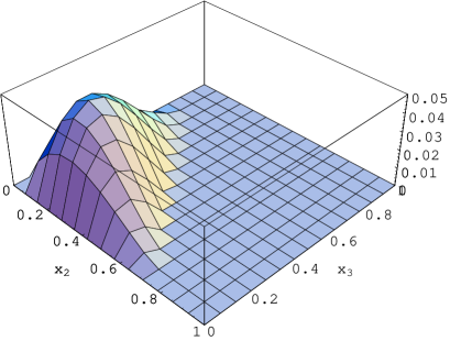
Figure 1: Twist-3 distribution amplitude $\Phi_{3}(x_{i})$

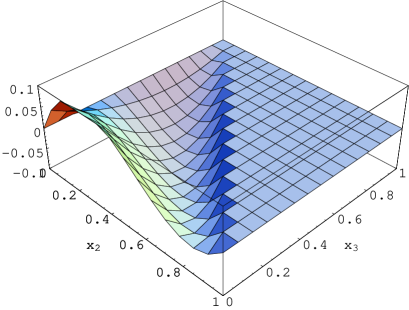
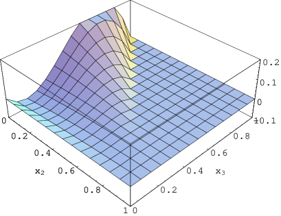
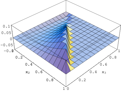
Figure 2: Twist-4 distribution amplitudes $\Phi_{4}(x_{i})$ in the first line to the left, $\Psi_{4}(x_{i})$ in the first line to the right, and $\Xi(x_{i})$ in the second line

4 Summary and conclusions

We have carried out a systematic study of the higher-twist light-cone distribution amplitudes of the nucleon in QCD and found that a generic three-quark matrix element on the light-cone can be parametrized in terms of eight independent nucleon distribution amplitudes. In particular, we have identified one distribution of leading twist-3, three of twist-4, three of twist-5 and one of twist-6. The shape of the distribution amplitudes at asymtotically large momentum transfers is found and is dictated by the conformal symmetry of the QCD Lagrangian. In order to quantify the corrections, we attempt to expand the distribution amplitudes in contributions of local conformal operators and keep contributions of the next-to-leading conformal spin (“P”-waves). The coefficients in this expansion present the necessary nonperturbative input. Some of them are related by QCD equations of motion, so that to our accuracy we end up with eight independent parameters

From this amount, three parameters determine the leading twist amplitude and are known already from the analysis in [11]; two more — the normalisations of the higher-twist asymptotic distributions — can be directly inferred from QCD sum rule phenomenology of the nucleon. The remaining three parameters determine the deviation of the higher-twist distribution amplitudes from their asymptotic form and are estimated in this work.

To avoid confusion, we remind that our work does not present the complete analysis of all existing higher-twist distributions, but of its subset related to three-quark operators without extra gluon fields. As explained in the introduction, we believe that the three-quark contributions considered in this paper dominate higher-twist corrections because of large matrix elements. Indeed, we found that the matrix elements of higher-twist three-quark operators are of the same order or larger than those of the leading twist, see Sec. 3. We stress that the situation in the nucleon case is quite different to that of higher twist-corrections in the meson case studied earlier [8, 9]. The reason is that in the meson case “bad” components of quark fields always can be eliminated in favour of “good” components and an additional gluon. The resulting matrix elements turn out to be numerical small. In the nucleon case quark fields with “minus” projection give rise to genuine three-quark higher twist effects that cannot be attributed to higher Fock components in the wave function, involving an additional gluon.

A detailed summary of the distribution amplitudes is presented in Appendix C. In this paper we do not consider phenomenological applications, but expect that our results are relevant for the studies of a wide range of interesting physical processes.

One obvious application can be found in the calculation of the nucleon form factors. While the magnetic form factor of the proton $G_{\rm M}(Q^{2})$ allows for the leading twist description [1, 3], it is known that the Pauli formfactor $F_{2}(Q^{2})$ is higher-twist, suppressed by an additional power of $Q^{2}$. The description of $F_{2}$ therefore calls for the input of higher twist distribution amplitudes presented in this paper.

Twist-4 distribution amplitudes of the nucleon are, probably, the most interesting and in general are related to various spin asymmetries in exclusive processes. Indeed, while the total helicity is conserved in processes involving leading twist distribution amplitdues [29], this is not the case for non-leading twist contributions. Thus spin-sensitive transition formfactors will provide a testing ground for higher twist effects.

Last but not least, the distribution amplitudes presented in this paper can immediately be applied to calculations of exclusive reactions at moderate momentum transfers in the framework of QCD light-cone sum rules [30]. This approach allows to study soft non-factorisable contributions to hard exclusive reactions in a largely model-independent way, see e.g. [31].

Appendices

Appendix A Fierz transformations

In this section we give the Fierz transformation rules necessary to derive the isospin constraints Eq. (2.2) from the symmetry requirement Eq. (2.29).

We write the definition of distribution amplitudes in Eq. (2.9) in a shorthand notation as

$$\left\langle 0\right|\varepsilon^{ijk}u_{\alpha}^{i}(a_{1}z)u_{\beta}^{j}(a_{2}z)d_{\gamma}^{k}(a_{3}z)\left|P(P,\lambda)\right\rangle$$

$$=S_{1}(s_{1})_{\alpha\beta,\gamma}+S_{2}(s_{2})_{\alpha\beta,\gamma}+P_{1}(p_{1})_{\alpha\beta,\gamma}+P_{2}(p_{2})_{\alpha\beta,\gamma}+V_{1}(v_{1})_{\alpha\beta,\gamma}+V_{2}(v_{2})_{\alpha\beta,\gamma}+\frac{1}{2}V_{3}(v_{3})_{\alpha\beta,\gamma}$$

$$+\frac{1}{2}V_{4}(v_{4})_{\alpha\beta,\gamma}+V_{5}(v_{5})_{\alpha\beta,\gamma}+V_{6}(v_{6})_{\alpha\beta,\gamma}+A_{1}(a_{1})_{\alpha\beta,\gamma}+A_{2}(a_{2})_{\alpha\beta,\gamma}+\frac{1}{2}A_{3}(a_{3})_{\alpha\beta,\gamma}$$

$$+\frac{1}{2}A_{4}(a_{4})_{\alpha\beta,\gamma}+A_{5}(a_{5})_{\alpha\beta,\gamma}+A_{6}(a_{6})_{\alpha\beta,\gamma}+T_{1}(t_{1})_{\alpha\beta,\gamma}+T_{2}(t_{2})_{\alpha\beta,\gamma}+T_{3}(t_{3})_{\alpha\beta,\gamma}$$

$$+T_{4}(t_{4})_{\alpha\beta,\gamma}+T_{5}(t_{5})_{\alpha\beta,\gamma}+\frac{1}{2}T_{7}(t_{7})_{\alpha\beta,\gamma}+\frac{1}{2}T_{8}(t_{8})_{\alpha\beta,\gamma}\,.$$ (A.1)

The small letters, e.g. $(s_{1})_{\alpha\beta,\gamma}=\left(C\right)_{\alpha\beta}N_{\gamma}$ stand for the Lorentz structures $\left(\Gamma C\right)_{\alpha\beta}\left(\Gamma^{\prime}N\right)_{\gamma}$, etc. By means of the following Fierz transformation

$$\left(\Gamma C\right)_{\alpha\beta}\left(\Gamma^{\prime}N\right)_{\gamma}=\frac{1}{4}\bigg{[}C_{\gamma\beta}\left(\Gamma\Gamma^{\prime}N\right)_{\alpha}+\left(\gamma_{5}C\right)_{\gamma\beta}\left(\Gamma\gamma_{5}\Gamma^{\prime}N\right)_{\alpha}$$

$$+\frac{1}{{p\cdot z}}\left(\!\not\!{p}C\right)_{\gamma\beta}\left(\Gamma\!\not\!{z}\Gamma^{\prime}N\right)_{\alpha}+\frac{1}{{p\cdot z}}\left(\!\not\!{z}C\right)_{\gamma\beta}\left(\Gamma\!\not\!{p}\Gamma^{\prime}N\right)_{\alpha}+\left(\gamma_{\perp}C\right)_{\gamma\beta}\left(\Gamma\gamma^{\perp}\Gamma^{\prime}N\right)_{\alpha}$$

$$-\frac{1}{{p\cdot z}}\left(\!\not\!{p}\gamma_{5}C\right)_{\gamma\beta}\left(\Gamma\!\not\!{z}\gamma_{5}\Gamma^{\prime}N\right)_{\alpha}-\frac{1}{{p\cdot z}}\left(\!\not\!{z}\gamma_{5}C\right)_{\gamma\beta}\left(\Gamma\!\not\!{p}\gamma_{5}\Gamma^{\prime}N\right)_{\alpha}-\left(\gamma_{\perp}\gamma_{5}C\right)_{\gamma\beta}\left(\Gamma\gamma^{\perp}\gamma_{5}\Gamma^{\prime}N\right)_{\alpha}$$

$$+\frac{1}{({p\cdot z})^{2}}\left(\sigma_{pz}C\right)_{\gamma\beta}\left(\Gamma\sigma_{zp}\Gamma^{\prime}N\right)_{\alpha}+\frac{1}{2}\left(\sigma_{\perp\perp^{\prime}}C\right)_{\gamma\beta}\left(\Gamma\sigma^{\perp\perp^{\prime}}\Gamma^{\prime}N\right)_{\alpha}$$

$$+\frac{1}{{p\cdot z}}\left(i\sigma_{\perp p}C\right)_{\gamma\beta}\left(\Gamma\gamma^{\perp}\!\not\!{z}\Gamma^{\prime}N\right)_{\alpha}+\frac{1}{{p\cdot z}}\left(i\sigma_{\perp z}C\right)_{\gamma\beta}\left(\Gamma\gamma^{\perp}\!\not\!{p}\Gamma^{\prime}N\right)_{\alpha}\bigg{]}$$ (A.2)

all Lorentz structures are brought into the same form, i.e. we apply for the expansion of the third contribution in Eq. (2.29) the following transformations of twist-3 structures

$$(v_{1})_{\gamma\beta,\alpha} = \frac{1}{2}\left(v_{1}-a_{1}-t_{1}\right)_{\alpha\beta,\gamma}$$

$$(a_{1})_{\gamma\beta,\alpha} = \frac{1}{2}\left(-v_{1}+a_{1}-t_{1}\right)_{\alpha\beta,\gamma}$$

$$(t_{1})_{\gamma\beta,\alpha} = -\left(v_{1}+a_{1}\right)_{\alpha\beta,\gamma}$$ (A.3)

and similar transformations for twist-4

$$(s_{1})_{\gamma\beta,\alpha} = \frac{1}{4}\left(s_{1}+p_{1}-2v_{2}-2a_{2}+v_{3}-a_{3}-t_{3}-2t_{2}+\frac{1}{2}t_{7}\right)_{\alpha\beta,\gamma}$$

$$(p_{1})_{\gamma\beta,\alpha} = \frac{1}{4}\left(s_{1}+p_{1}+2v_{2}+2a_{2}-v_{3}+a_{3}-t_{3}-2t_{2}+\frac{1}{2}t_{7}\right)_{\alpha\beta,\gamma}$$

$$(v_{2})_{\gamma\beta,\alpha} = \frac{1}{4}\left(-s_{1}+p_{1}+v_{3}+a_{3}-t_{3}-\frac{1}{2}t_{7}\right)_{\alpha\beta,\gamma}$$

$$(a_{2})_{\gamma\beta,\alpha} = \frac{1}{4}\left(-s_{1}+p_{1}-v_{3}-a_{3}-t_{3}-\frac{1}{2}t_{7}\right)_{\alpha\beta,\gamma}$$

$$(v_{3})_{\gamma\beta,\alpha} = \frac{1}{4}\left(2s_{1}-2p_{1}+4v_{2}-4a_{2}-2t_{3}-t_{7}\right)_{\alpha\beta,\gamma}$$

$$(a_{3})_{\gamma\beta,\alpha} = \frac{1}{4}\left(-2s_{1}+2p_{1}+4v_{2}-4a_{2}+2t_{3}+t_{7}\right)_{\alpha\beta,\gamma}$$

$$(t_{2})_{\gamma\beta,\alpha} = \frac{1}{4}\left(-2s_{1}-2p_{1}-2t_{3}+t_{7}\right)_{\alpha\beta,\gamma}$$

$$(t_{3})_{\gamma\beta,\alpha} = \frac{1}{4}\left(-s_{1}-p_{1}-2v_{2}-2a_{2}-v_{3}+a_{3}+t_{3}-2t_{2}-\frac{1}{2}t_{7}\right)_{\alpha\beta,\gamma}$$

$$(t_{7})_{\gamma\beta,\alpha} = \frac{1}{4}\left(2s_{1}+2p_{1}-4v_{2}-4a_{2}-2v_{3}+2a_{3}-2t_{3}+4t_{2}+t_{7}\right)_{\alpha\beta,\gamma}\,.$$ (A.4)

Relations for twist-5 and twist-6 are identical up to the substitutions: $\{v_{1},a_{1},t_{1}\}\to\{v_{6},a_{6},t_{6}\}$ and $\{s_{1},p_{1},v_{2},v_{3},a_{2},a_{3},t_{2},t_{3},t_{7}\}\to\{s_{2},p_{2},v_{5},v_{4},a_{5},a_{4},t_{5},t_{4},t_{8}\}$. By a simple substitution, one also gets the necessary Fierz transformations from $(\ldots)_{\alpha\gamma,\beta}\to(\ldots)_{\alpha\beta,\gamma}$ required in the second contribution in Eq. (2.29). Putting everything together we derive three equations for the twist-3 amplitudes from the coefficients $v_{1},a_{1},t_{1}$:

$$0=\left[2T_{1}(1,2,3)-V_{1}(1,3,2)+A_{1}(1,3,2)-V_{1}(3,2,1)-A_{1}(3,2,1)\right]\left(t_{1}\right)_{\alpha\beta,\gamma}$$

$$+\left[2V_{1}(1,2,3)+2V_{1}(1,3,2)+2A_{1}(1,3,2)-2T_{1}(1,3,2)\right.$$

$$\left.\quad+V_{1}(3,2,1)-A_{1}(3,2,1)-2T_{1}(3,2,1)\right]\left(v_{1}\right)_{\alpha\beta,\gamma}$$

$$+\left[2A_{1}(1,2,3)+2V_{1}(1,3,2)+2A_{1}(1,3,2)+2T_{1}(1,3,2)\right.$$

$$\left.\quad-V_{1}(3,2,1)+A_{1}(3,2,1)-2T_{1}(3,2,1)\right]\left(a_{1}\right)_{\alpha\beta,\gamma}\,.$$ (A.5)

Using the symmetry properties Eq. (2.28) it is easy to see, however, that all three above equations are in fact identical to the one given in Eq. (2.2). In the similar way one can derive an overcomplete set of nine twist-4 equations that all can be reduced to the two equations relating twist-4 amplitudes in Eq. (2.2). The derivation for the remaining twist-5 and twist-6 equations is similar.

Appendix B Nonperturbative parameters

In Sect. 3.2 we have demonstrated that the normalisation of the asymptotic distribution amplitudes of all twists involves three independent parameters. In the first part of this Appendix we consider leading corrections to the asymptotic distribution amplitudes, related to contributions of three-quark conformal one extra derivative, and find that they involve five new parameters.

In the second part, we work out QCD sum rule estimates of the higher-twist matrix elements. Partially the results can be adapted from existing sum rule calculations containing nucleon currents [12, 14, 28], partially they are new.

B.1 Equations of motion

The coefficients of “P”-wave contributions in the conformal expansion of distribution amplitudes are given by matrix elements of operators containing one derivative. In case the derivative acts on the down quark we have the general decomposition:

$$4\left\langle 0\right|\varepsilon^{ijk}u_{\alpha}^{i}(0)u_{\beta}^{j}(0)\left[iD_{\lambda}d_{\gamma}\right]^{k}(0)\left|N,P\right\rangle$$

$$={\cal V}_{1}^{d}P_{\lambda}\left(\!\not\!{P}C\right)_{\alpha\beta}\left(\gamma_{5}N\right)_{\gamma}+{\cal V}_{2}^{0}M\left(\!\not\!{P}C\right)_{\alpha\beta}\left(\gamma_{\lambda}\gamma_{5}N\right)_{\gamma}+{\cal V}_{3}^{d}P_{\lambda}M\left(\gamma_{\mu}C\right)_{\alpha\beta}\left(\gamma^{\mu}\gamma_{5}N\right)_{\gamma}$$

$$+{\cal V}_{4}^{0}M^{2}\left(\gamma_{\lambda}C\right)_{\alpha\beta}\left(\gamma_{5}N\right)_{\gamma}+{\cal V}_{5}^{0}M^{2}\left(\gamma^{\mu}C\right)_{\alpha\beta}\left(i\sigma_{\mu\lambda}\gamma_{5}N\right)_{\gamma}$$

$$+{\cal T}_{1}^{d}P_{\lambda}\left(P^{\nu}i\sigma_{\mu\nu}C\right)_{\alpha\beta}\left(\gamma^{\mu}\gamma_{5}N\right)_{\gamma}+{\cal T}_{2}^{0}M\left(P^{\nu}i\sigma_{\lambda\nu}C\right)_{\alpha\beta}\left(\gamma_{5}N\right)_{\gamma}+{\cal T}_{3}^{d}P_{\lambda}M\left(\sigma_{\mu\nu}C\right)_{\alpha\beta}\left(\sigma^{\mu\nu}\gamma_{5}N\right)_{\gamma}$$

$$+{\cal T}_{4}^{0}M\left(P_{\nu}\sigma^{\mu\nu}C\right)_{\alpha\beta}\left(\sigma_{\mu\lambda}\gamma_{5}N\right)_{\gamma}+{\cal T}_{5}^{0}M^{2}\left(i\sigma_{\mu\lambda}C\right)_{\alpha\beta}\left(\gamma^{\mu}\gamma_{5}N\right)_{\gamma}$$

$$+{\cal T}_{7}^{0}M^{2}\left(\sigma_{\mu\nu}C\right)_{\alpha\beta}\left(\sigma^{\mu\nu}\gamma_{\lambda}\gamma_{5}N\right)_{\gamma}$$ (B.1)

yielding 11 parameters.

Acting with one derivative on the up-quarks picks up the structures of $\gamma$-matrices that are odd under transposition:

$$4\left\langle 0\right|\varepsilon^{ijk}u_{\alpha}^{i}(0)i\stackrel{{\scriptstyle\leftrightarrow}}{{D}}_{\lambda}u_{\beta}^{j}(0)d_{\gamma}^{k}(0)\left|N,P\right\rangle$$

$$={\cal S}_{1}^{u}P_{\lambda}MC_{\alpha\beta}\left(\gamma_{5}N\right)_{\gamma}+{\cal S}_{2}^{0}M^{2}C_{\alpha\beta}\left(\gamma_{\lambda}\gamma_{5}N\right)_{\gamma}+$$

$$+{\cal P}_{1}^{u}P_{\lambda}M\left(\gamma_{5}C\right)_{\alpha\beta}N_{\gamma}+{\cal P}_{2}^{0}M^{2}\left(\gamma_{5}C\right)_{\alpha\beta}\left(\gamma_{\lambda}N\right)_{\gamma}+$$

$$+{\cal A}_{1}^{u}P_{\lambda}\left(\!\not\!{P}\gamma_{5}C\right)_{\alpha\beta}N_{\gamma}+{\cal A}_{2}^{0}M\left(\!\not\!{P}\gamma_{5}C\right)_{\alpha\beta}\left(\gamma_{\lambda}N\right)_{\gamma}+{\cal A}_{3}^{u}P_{\lambda}M\left(\gamma_{\mu}\gamma_{5}C\right)_{\alpha\beta}\left(\gamma^{\mu}N\right)_{\gamma}$$

$$+{\cal A}_{4}^{0}M^{2}\left(\gamma_{\lambda}\gamma_{5}C\right)_{\alpha\beta}N_{\gamma}+{\cal A}_{5}^{0}M^{2}\left(\gamma^{\mu}\gamma_{5}C\right)^{\alpha\beta}\left(i\sigma_{\mu\lambda}N\right)_{\gamma}$$ (B.2)

and introduces 9 parameters. Hence, altogether there are 20 unknown numbers. The equations of motions yield, however, a number of constraints:

$$\left\langle 0\right|\varepsilon^{ijk}u^{i}(0)C\gamma_{\varrho}u^{j}(0)\,\gamma^{\lambda}\left[iD_{\lambda}d_{\gamma}\right]^{k}(0)\left|N,P\right\rangle=0\,,$$

$$\left\langle 0\right|\varepsilon^{ijk}u^{i}(0)C\gamma^{\lambda}u^{j}(0)\,\left[iD_{\lambda}d_{\gamma}\right]^{k}(0)\left|N,P\right\rangle=P_{\lambda}\left\langle 0\right|\varepsilon^{ijk}u^{i}(0)C\gamma_{\lambda}u^{j}(0)\,d_{\gamma}^{k}(0)\left|N,P\right\rangle\,,$$

$$\left\langle 0\right|\varepsilon^{ijk}u^{i}(0)C\sigma_{\alpha\beta}u^{j}(0)\,\gamma^{\lambda}\left[iD_{\lambda}d_{\gamma}\right]^{k}(0)\left|N,P\right\rangle=0\,,$$

$$\left\langle 0\right|\varepsilon^{ijk}u^{i}(0)Ci\sigma_{\alpha\beta}u^{j}(0)\,\left[iD^{\beta}d_{\gamma}\right]^{k}(0)\left|N,P\right\rangle$$

$$=P^{\beta}\left\langle 0\right|\varepsilon^{ijk}u^{i}(0)Ci\sigma_{\alpha\beta}u^{j}(0)\,d^{k}(0)\left|N,P\right\rangle-\left\langle 0\right|\varepsilon^{ijk}\left[u(0)Ci\stackrel{{\scriptstyle\leftrightarrow}}{{D}}_{\alpha}u(0)\right]^{ij}\,d_{\gamma}^{k}(0)\left|N,P\right\rangle\,,$$

$$\left\langle 0\right|\varepsilon^{ijk}u^{i}(0)Ci\gamma_{5}\sigma_{\alpha\beta}u^{j}(0)\,\,\left[iD^{\beta}d_{\gamma}\right]^{k}(0)\left|N,P\right\rangle$$

$$=P^{\beta}\left\langle 0\right|\varepsilon^{ijk}u^{i}(0)C\gamma_{5}i\sigma_{\alpha\beta}u^{j}(0)\,d^{k}(0)\left|N,P\right\rangle-\left\langle 0\right|\varepsilon^{ijk}\left[u(0)C\gamma_{5}i\stackrel{{\scriptstyle\leftrightarrow}}{{D}}_{\alpha}u(0)\right]^{ij}\,d_{\gamma}^{k}(0)\left|N,P\right\rangle\,,$$

which translate to

$${\cal V}_{1}^{d} = 4{\cal V}_{2}^{0}+2{\cal V}_{3}^{d}\,,\hskip 22.76228pt\qquad-3{\cal V}_{5}^{0}={\cal V}_{3}^{d}+{\cal V}_{4}^{0}\,,$$

$${\cal V}_{1}^{0}-{\cal V}_{3}^{0} = {\cal V}_{1}^{d}-{\cal V}_{3}^{d}+4{\cal V}_{4}^{0}-{\cal V}_{2}^{0}\,,$$

$$0 = {\cal T}_{3}^{d}+{\cal T}_{5}^{0}\,,\hskip 45.52458pt\qquad{\cal T}_{2}^{0}=-{\cal T}_{1}^{d}+4{\cal T}_{3}^{d}+3{\cal T}_{4}^{0}\,,$$

$${\cal T}_{1}^{0}-2{\cal T}_{3}^{0}-{\cal S}_{2}^{0} = {\cal T}_{1}^{d}-2{\cal T}_{3}^{d}-{\cal T}_{4}^{0}+3{\cal T}_{5}^{0}+6{\cal T}_{7}^{0}\,,$$

$${\cal T}_{1}^{0}-2{\cal T}_{3}^{0}-{\cal S}_{1}^{u} = {\cal T}_{1}^{d}-3{\cal T}_{2}^{0}-2{\cal T}_{3}^{d}-{\cal T}_{4}^{0}\,,$$

$$-2{\cal T}_{3}^{d}+2{\cal T}_{4}^{0} = -2{\cal T}_{3}^{0}-{\cal P}_{1}^{u}\,,\hskip 8.5359pt\quad 2{\cal T}_{3}^{0}-{\cal P}_{2}^{0}=2{\cal T}_{3}^{d}-2{\cal T}_{4}^{0}-6{\cal T}_{7}^{0}\,,$$ (B.4)

The two relations in the first line in Eq. (B.1) follow from the first equation in Eq. (B.1), the relations in the second line from the second equation, the third line from the third equation, fourth and fifth line from the fourth equation and the last line from the last equation. In a similar way one observes that the axial structures have to fulfill the constraints

$$\left\langle 0\right|\varepsilon^{ijk}\left[u(0)C\gamma^{\varrho}\gamma_{5}\stackrel{{\scriptstyle\leftrightarrow}}{{D}}_{\varrho}u(0)\right]^{ij}\,d_{\gamma}^{k}(0)\left|N,P\right\rangle=0\,,$$

$$\left\langle 0\right|\varepsilon^{ijk}\left[u(0)C\left\{\gamma_{\lambda}i\stackrel{{\scriptstyle\leftrightarrow}}{{D}}_{\varrho}-\gamma_{\varrho}i\stackrel{{\scriptstyle\leftrightarrow}}{{D}}_{\lambda}\right\}\gamma_{5}u(0)\right]^{ij}d_{\gamma}^{k}(0)\left|N,P\right\rangle$$

$$=\left\langle 0\right|\varepsilon^{ijk}\left[u(0)C\frac{i}{2}\left\{\sigma_{\lambda\varrho}\gamma^{\alpha}i\overleftarrow{D}_{\alpha}+\gamma^{\alpha}\sigma_{\lambda\varrho}i\overrightarrow{D}_{\alpha}\right\}\gamma_{5}u(0)\right]^{ij}\,d_{\gamma}^{k}(0)\left|N,P\right\rangle$$

$$=-i\varepsilon_{\lambda\varrho\alpha\delta}\left[P^{\alpha}\left\langle 0\right|\varepsilon^{ijk}u^{i}(0)C\gamma^{\delta}u^{j}(0)d_{\gamma}^{k}(0)\left|N,P\right\rangle-\left\langle 0\right|\varepsilon^{ijk}u^{i}(0)C\gamma^{\delta}u^{j}(0)\left[iD^{\alpha}d_{\gamma}\right]^{k}(0)\left|N,P\right\rangle\right]\,,$$

where from it follows that

$${\cal A}_{1}^{u}+{\cal A}_{3}^{u}+{\cal A}_{2}^{0}+4{\cal A}_{4}^{0}=0\,,$$

$${\cal A}_{3}^{u}-{\cal A}_{2}^{0}={\cal V}_{2}^{0}+{\cal V}_{3}^{0}-{\cal V}_{3}^{d}\,,\qquad 2{\cal A}_{5}^{0}={\cal V}_{2}^{0}+{\cal V}_{3}^{0}-2{\cal V}_{5}^{0}-{\cal V}_{3}^{d}\,.$$ (B.6)

where the relation in the first line is derived from the first equation in Eq. (B.1). Combining the constraints from the equations of motion with the eight isospin relations obtainable from Eq. (2.2) we obtain an overcomplete set of 20 equations. Choosing ${\cal V}_{1}^{d},{\cal A}_{1}^{u},{\cal V}_{3}^{d},{\cal A}_{3}^{u}$ and ${\cal T}_{3}^{d}$ as the independent parameters and solving these equations, we can express the remaining parameters as

$${\cal V}_{2}^{0}=\frac{1}{4}\left({\cal V}_{1}^{d}-2\,{\cal V}_{3}^{d}\right)\,,\qquad\hskip 119.50148pt{\cal V}_{4}^{0}=\frac{1}{16}\left(4\,{\cal V}_{1}^{0}-3\,{\cal V}_{1}^{d}-4\,{\cal V}_{3}^{0}+2\,{\cal V}_{3}^{d}\right)\,,$$

$${\cal V}_{5}^{0}=\frac{1}{48}\left(-4\,{\cal V}_{1}^{0}+3\,{\cal V}_{1}^{d}+4\,{\cal V}_{3}^{0}-18\,{\cal V}_{3}^{d}\right)\,,\qquad\hskip 25.6073pt{\cal A}_{2}^{0}={\cal A}_{3}^{u}-\frac{{\cal V}_{1}^{d}}{4}-{\cal V}_{3}^{0}+\frac{3\,{\cal V}_{3}^{d}}{2}\,,$$

$${\cal A}_{4}^{0}=\frac{1}{16}\left(-4\,{\cal A}_{1}^{u}-8\,{\cal A}_{3}^{u}+{\cal V}_{1}^{d}+4\,{\cal V}_{3}^{0}-6\,{\cal V}_{3}^{d}\right)\,,\qquad{\cal A}_{5}^{0}=\frac{1}{48}\left(4\,{\cal V}_{1}^{0}+3\,{\cal V}_{1}^{d}+20\,{\cal V}_{3}^{0}-18\,{\cal V}_{3}^{d}\right)\,,$$

$${\cal T}_{2}^{0}=\frac{1}{8}\left({\cal A}_{1}^{u}+6\,{\cal A}_{3}^{u}+8\,{\cal T}_{3}^{d}-{\cal V}_{1}^{0}-2\,{\cal V}_{1}^{d}-6\,{\cal V}_{3}^{0}+12\,{\cal V}_{3}^{d}\right)\,,\qquad{\cal T}_{5}^{0}=-{\cal T}_{3}^{d}\,,$$

$${\cal T}_{4}^{0}=\frac{1}{8}\left(-{\cal A}_{1}^{u}+2\,{\cal A}_{3}^{u}-8\,{\cal T}_{3}^{d}+{\cal V}_{1}^{0}-2\,{\cal V}_{1}^{d}-2\,{\cal V}_{3}^{0}+4\,{\cal V}_{3}^{d}\right)\,,$$

$${\cal T}_{7}^{0}=\frac{1}{96}\left(3\,{\cal A}_{1}^{u}-6\,{\cal A}_{3}^{u}-16\,{\cal T}_{3}^{0}+48\,{\cal T}_{3}^{d}+{\cal V}_{1}^{0}+6\,{\cal V}_{1}^{d}+6\,{\cal V}_{3}^{0}-12\,{\cal V}_{3}^{d}\right)\,,$$

$${\cal S}_{2}^{0}=\frac{1}{16}\left(3\,{\cal A}_{1}^{u}+10\,{\cal A}_{3}^{u}-16\,{\cal T}_{3}^{0}+16\,{\cal T}_{3}^{d}+9\,{\cal V}_{1}^{0}-2\,{\cal V}_{1}^{d}-10\,{\cal V}_{3}^{0}+20\,{\cal V}_{3}^{d}\right)\,,$$

$${\cal S}_{1}^{u}=\frac{1}{4}\left(3\,{\cal A}_{1}^{u}+10\,{\cal A}_{3}^{u}-8\,{\cal T}_{3}^{0}+16\,{\cal T}_{3}^{d}+{\cal V}_{1}^{0}-2\,{\cal V}_{1}^{d}-10\,{\cal V}_{3}^{0}+20\,{\cal V}_{3}^{d}\right)\,,$$

$${\cal P}_{1}^{u}=\frac{1}{4}\left({\cal A}_{1}^{u}-2\,{\cal A}_{3}^{u}-8\,{\cal T}_{3}^{0}+16\,{\cal T}_{3}^{d}-{\cal V}_{1}^{0}+2\,{\cal V}_{1}^{d}+2\,{\cal V}_{3}^{0}-4\,{\cal V}_{3}^{d}\right)\,,$$

$${\cal P}_{2}^{0}=\frac{1}{16}\left(-{\cal A}_{1}^{u}+2\,{\cal A}_{3}^{u}+16\,{\cal T}_{3}^{0}-16\,{\cal T}_{3}^{d}+5\,{\cal V}_{1}^{0}-2\,{\cal V}_{1}^{d}-2\,{\cal V}_{3}^{0}+4\,{\cal V}_{3}^{d}\right)\,,$$

$${\cal T}_{1}^{d}=\frac{1}{2}\left(-{\cal A}_{1}^{u}+{\cal V}_{1}^{0}-{\cal V}_{1}^{d}\right)\,.$$ (B.7)

Finally, the parameters ${\cal V}_{1}^{d},{\cal A}_{1}^{u},{\cal V}_{3}^{d},{\cal A}_{3}^{u}$ and ${\cal T}_{3}^{d}$ can be expressed by the reduced matrix elements of the operators defined in Eq. (3.2). We have

$${\cal V}_{1}^{d} = f_{N}V_{1}^{d}\,,\qquad{\cal A}_{1}^{u}=f_{N}A_{1}^{u}\,,\qquad\lambda_{1}f_{1}^{d}=\frac{1}{2}\left({\cal V}_{1}^{d}-6{\cal V}_{3}^{d}\right)\,,$$

$$\lambda_{1}f_{1}^{u} = \frac{1}{2}\left(-2{\cal A}_{1}^{u}-12{\cal A}_{3}^{u}+{\cal V}_{1}^{d}+4{\cal V}_{3}^{0}-6{\cal V}_{3}^{d}\right)\,,$$

$$\lambda_{2}f_{2}^{d} = 2\left(-2{\cal A}_{3}^{u}-8{\cal T}_{3}^{d}+{\cal V}_{1}^{d}+2{\cal V}_{3}^{0}-4{\cal V}_{3}^{d}+2{\cal T}_{1}^{d}\right)\,.$$ (B.8)

The first two parameters appear already at the level of twist-3 and are known from [11]. The others will be calculated in the next subsection.

B.2 QCD sum rule estimates

The QCD sum rule estimates for $\lambda_{1}$, $\lambda_{2}$ are derived from the consideration of the two-point correlation function

$$i\int{\rm d}^{4}x\,e^{iqx}\left\langle 0\right|\eta_{i}(x)\bar{\eta}_{i}(0)\left|0\right\rangle=|\lambda_{i}|^{2}M^{2}\frac{(\!\not\!{q}+M)}{M^{2}-q^{2}}+\ldots\,,$$ (B.9)

where $\left\langle 0\right|\eta_{1}(0)\left|P\right\rangle=M\lambda_{1}N(P)$ and $\left\langle 0\right|\eta_{2}(0)\left|P\right\rangle=M\lambda_{2}N(P)$ are the local three-quark operators defined in Eq. (3.2). The dots refer to excited states and the continuum contribution. Taking into account vacuum condensates up to dimension-8 one obtains the sum rules [14, 28]:

$$2(2\pi)^{4}M^{2}|\lambda_{1}|^{2} = \exp(M^{2}/M_{B}^{2})\left\{M_{B}^{6}E_{3}(s_{0}/M_{B}^{2})+\frac{b}{4}M_{B}^{2}E_{1}(s_{0}/M_{B}^{2})+\frac{a^{2}}{3}\left(4-\frac{m_{0}^{2}}{M_{B}^{2}}\right)\right\}$$

and

$$2(2\pi)^{4}M^{2}\frac{|\lambda_{2}|^{2}}{6} = \exp(M^{2}/M_{B}^{2})\left\{M_{B}^{6}E_{3}(s_{0}/M_{B}^{2})+\frac{b}{4}M_{B}^{2}E_{1}(s_{0}/M_{B}^{2})\right\}\,,$$ (B.11)

where

$$E_{n}(s_{0}/M_{B}^{2})=1-e^{(-s_{0}/M_{B}^{2})}\sum_{k=0}^{n-1}\frac{1}{k!}\left(\frac{s_{0}}{M_{B}^{2}}\right)^{k}\,.$$ (B.12)

Here and below $M_{B}$ is the Borel parameter. We use the Borel window $1{\rm GeV^{2}}\leq M_{B}^{2}\leq 2{\rm GeV^{2}}$, with the continuum threshold $\sqrt{s_{0}}\sim 1.5\;{\rm GeV}$ and values of the condensates normalized at $\mu^{2}=1~{}{\rm GeV^{2}}$ [9]:

$$a = -(2\pi)^{2}\langle\bar{q}q\rangle~{}~{}~{}~{}~{}\sim 0.55\;{\rm GeV^{3}}\,,$$

$$b = \phantom{-}(2\pi)^{2}\langle\frac{\alpha_{S}}{\pi}G^{2}\rangle\sim 0.47\;{\rm GeV^{4}}\,,$$

$$m_{0}^{2} = \phantom{-}\frac{\langle\bar{q}gGq\rangle}{\langle\bar{q}q\rangle}~{}~{}~{}~{}~{}~{}~{}~{}\sim 0.8\;{\rm GeV^{2}}\,.$$ (B.13)

With these inputs, we find $|\lambda_{1}|=0.027\pm 0.009\,{\rm GeV^{2}}$, $|\lambda_{2}|=0.051\pm 0.019\,{\rm GeV^{2}}$. Note that the above sum rules only fix the absolute value of the parameters $\lambda_{1}$ and $\lambda_{2}$. Relative phases between different nucleon-to-vacuum matrix elements can be computed by investigating suitable non-diagonal correlation functions. To determine the relative sign between $f_{N}$ and $\lambda_{1}$ we consider the correlation function

$$i\int{\rm d}^{4}x\,e^{iqx}\left\langle 0\right|\varepsilon^{ijk}\left[u^{i}(x)C\!\not\!{z}u^{j}(x)\right]\,\gamma_{5}\!\not\!{z}d^{k}(x)\;\bar{\eta}_{1}(0)\left|0\right\rangle=f_{N}\lambda_{1}^{*}M\!\not\!{z}\frac{(\!\not\!{q}+M)}{M^{2}-q^{2}}+\ldots\,.$$ (B.14)

Taking the ratio of the corresponding sum rule and the sum rule Eq. (B.2) we obtain

$$\frac{f_{N}}{\lambda_{1}}=-\frac{1}{3}\frac{\left(2M_{B}^{2}E_{1}(s_{0}/M_{B}^{2})-m_{0}^{2}\right)aM}{\displaystyle M_{B}^{6}E_{3}(s_{0}/M_{B}^{2})+\frac{b}{4}M_{B}^{2}E_{1}(s_{0}/M_{B}^{2})+\frac{a^{2}}{3}\left(4-\frac{m_{0}^{2}}{M_{B}^{2}}\right)}$$ (B.15)

which is real and negative. We have chosen $f_{N}$ to be positive according to the standard choice in [11] and $\lambda_{1}$ to be negative. Note also that the above sum rule leads to a value $f_{N}=5.6\cdot 10^{-3}{\rm GeV^{2}}$ consistent with standard estimates. A similar calculation of the nondiagonal correlation function

$$i\int{\rm d}^{4}x\,e^{iqx}\left\langle 0\right|\eta_{1}(x)\bar{\eta}_{2}(0)+\eta_{2}(x)\bar{\eta}_{1}(0)\left|0\right\rangle=\left(\lambda_{1}\lambda_{2}^{*}+\lambda_{2}\lambda_{1}^{*}\right)M^{2}\frac{(\!\not\!{q}+M)}{M^{2}-q^{2}}+\ldots$$ (B.16)

was performed in [14]. The resulting sum rule

$$-2(2\pi)^{4}M^{3}\left(\lambda_{1}\lambda_{2}^{*}+\lambda_{2}\lambda_{1}^{*}\right)=2ae^{\frac{M^{2}}{M_{B}^{2}}}\left(12M_{B}^{4}E_{2}(s_{0}/M_{B}^{2})-6m_{0}^{2}M_{B}^{2}E_{1}(s_{0}/M_{B}^{2})+\frac{32\alpha_{s}a^{2}}{27\pi M_{B}^{2}}\right)$$

shows that the relative sign between $\lambda_{2}$ and $\lambda_{1}$ is negative.

To estimate the remaining parameters we consider the nondiagonal correlation functions involving the last three higher-twist operators in Eq. (3.2) with either $\bar{\eta}_{1}(0)$ or $\bar{\eta}_{2}(0)$:

$$i\int{\rm d}^{4}x\,e^{iqx}\left\langle 0\right|\varepsilon^{ijk}\left(u^{i}(x)C\gamma_{\mu}u^{j}(x)\right)\,\gamma_{5}\gamma^{\mu}(iz\overrightarrow{D}d)^{k}(x)\;\bar{\eta}_{1}(0)\left|0\right\rangle=\frac{f_{1}^{d}|\lambda_{1}|^{2}M^{2}q\cdot z\!\not\!{q}}{M^{2}-q^{2}}+\ldots\,,$$

$$i\int{\rm d}^{4}x\,e^{iqx}\left\langle 0\right|\varepsilon^{ijk}\left(u(x)C\gamma_{\mu}\gamma_{5}iz\stackrel{{\scriptstyle\leftrightarrow}}{{D}}u(x)\right)^{ij}\,\gamma^{\mu}d^{k}(x)\;\bar{\eta}_{1}(0)\left|0\right\rangle=\frac{f_{1}^{u}|\lambda_{1}|^{2}M^{2}q\cdot z\!\not\!{q}}{M^{2}-q^{2}}+\ldots\,,$$

$$i\int{\rm d}^{4}x\,e^{iqx}\varepsilon^{ijk}\left\langle 0\right|\left(u^{i}(x)C\sigma_{\mu\nu}u^{j}(x)\right)\,\gamma_{5}\sigma^{\mu\nu}(iz\overrightarrow{D}d)^{k}(x)\;\bar{\eta}_{2}(0)\left|0\right\rangle=\frac{f_{2}^{d}|\lambda_{2}|^{2}M^{2}q\cdot z\!\not\!{q}}{M^{2}-q^{2}}+\ldots\,.$$

The dots refer, again, to contributions of excited states and different Lorentz structures that we do not consider. Expressing $|\lambda_{i}|^{2}$ by the expression in Eq. (B.2) and Eq. (B.11) we obtain the following sum rules:

$$f_{1}^{d} = \frac{\displaystyle\frac{3}{10}M_{B}^{6}E_{3}(s_{0}/M_{B}^{2})+\frac{b}{9}M_{B}^{2}E_{1}(s_{0}/M_{B}^{2})+\frac{a^{2}}{3}\left(4-\frac{m_{0}^{2}}{M_{B}^{2}}\right)}{\displaystyle M_{B}^{6}E_{3}(s_{0}/M_{B}^{2})+\frac{b}{4}M_{B}^{2}E_{1}(s_{0}/M_{B}^{2})+\frac{a^{2}}{3}\left(4-\frac{m_{0}^{2}}{M_{B}^{2}}\right)}\,,$$

$$f_{1}^{u} = \frac{\displaystyle\frac{1}{10}M_{B}^{6}E_{3}(s_{0}/M_{B}^{2})+\frac{b}{8}M_{B}^{2}E_{1}(s_{0}/M_{B}^{2})+\frac{5a^{2}}{18}\frac{m_{0}^{2}}{M_{B}^{2}}}{\displaystyle M_{B}^{6}E_{3}(s_{0}/M_{B}^{2})+\frac{b}{4}M_{B}^{2}E_{1}(s_{0}/M_{B}^{2})+\frac{a^{2}}{3}\left(4-\frac{m_{0}^{2}}{M_{B}^{2}}\right)}\,,$$

$$f_{2}^{d} = \frac{\displaystyle\frac{8}{5}M_{B}^{6}E_{3}(s_{0}/M_{B}^{2})-\frac{4b}{9}M_{B}^{2}E_{1}(s_{0}/M_{B}^{2})}{\displaystyle 6M_{B}^{6}E_{3}(s_{0}/M_{B}^{2})+\frac{3b}{2}M_{B}^{2}E_{1}(s_{0}/M_{B}^{2})}\,.$$ (B.19)

Inserting the numerical values of parameters, we end up with the following estimates for the higher-twist matrix elements:

$$f_{1}^{d}(\mu=1~{}{\rm GeV}) = 0.6\pm 0.2\,,$$

$$f_{2}^{d}(\mu=1~{}{\rm GeV}) = 0.15\pm 0.06\,,$$

$$f_{1}^{u}(\mu=1~{}{\rm GeV}) = 0.22\pm 0.15\,.$$ (B.20)

Appendix C Handbook of nucleon distribution amplitudes

In this Appendix we give a complete list of all 24 nucleon distribution amplitudes.

The chiral structure of our basic set of eight independent distribution amplitudes is summarized in Table 2 in the text. The corresponding representations for the remaining 16 distributions are collected in Table A and Table B. The set in Table A contains the amplitudes that can be directly obtained from Eq. (2.38) to Eq. (2.41) by flipping spin-projections of the two up-quarks. Table B contains four distributions that are obtainable from the previous ones by exchanging light-cone projections, and also $T_{1},T_{2},T_{5}$ and $T_{6}$ that cannot be read off from the previous expressions in a straightforward way and therefore are given below:

$$\left\langle 0\right|\varepsilon^{ijk}\!\left(u^{{\uparrow}}_{i}(a_{1}z)Ci\sigma_{\perp z}u^{{\uparrow}}_{j}(a_{2}z)\right)\gamma^{\perp}\!\not\!{z}d^{{\downarrow}}_{k}(a_{3}z)\left|P\right\rangle = -2pz\!\not\!{z}N^{\uparrow}\!\!\int\!\!{\cal D}x\,e^{-ipz\sum x_{i}a_{i}}\,T_{1}(x_{i})\,,$$

$$\left\langle 0\right|\varepsilon^{ijk}\!\left(u^{{\downarrow}}_{i}(a_{1}z)Ci\sigma_{\perp z}u^{{\downarrow}}_{j}(a_{2}z)\right)\gamma^{\perp}\!\not\!{p}d^{{\downarrow}}_{k}(a_{3}z)\left|P\right\rangle = -2pz\!\not\!{p}N^{\uparrow}\!\!\int\!\!{\cal D}x\,e^{-ipz\sum x_{i}a_{i}}\,T_{2}(x_{i})\,,$$

$$\left\langle 0\right|\varepsilon^{ijk}\!\left(u^{{\downarrow}}_{i}(a_{1}z)Ci\sigma_{\perp p}u^{{\downarrow}}_{j}(a_{2}z)\right)\gamma^{\perp}\!\not\!{z}d^{{\downarrow}}_{k}(a_{3}z)\left|P\right\rangle = -M^{2}\!\not\!{z}N^{\uparrow}\!\!\int\!\!{\cal D}x\,e^{-ipz\sum x_{i}a_{i}}\,T_{5}(x_{i})\,,$$

$$\left\langle 0\right|\varepsilon^{ijk}\!\left(u^{{\uparrow}}_{i}(a_{1}z)Ci\sigma_{\perp p}u^{{\uparrow}}_{j}(a_{2}z)\right)\gamma^{\perp}\!\not\!{p}d^{{\downarrow}}_{k}(a_{3}z)\left|P\right\rangle = -M^{2}\!\not\!{p}N^{\uparrow}\!\!\int\!\!{\cal D}x\,e^{-ipz\sum x_{i}a_{i}}\,T_{6}(x_{i})\,.$$ (C.1)

Note also that for scalar and tensor contributions the following representations can be given:

$$\left\langle 0\right|\varepsilon^{ijk}\!\left(u^{{\uparrow}}_{i}(a_{1}z)Cu^{{\uparrow}}_{j}(a_{2}z)\right)\!\not\!{z}d^{{\uparrow}}_{k}(a_{3}z)\left|P\right\rangle = \frac{1}{2}M\!\not\!{z}N^{\uparrow}\!\!\int\!\!{\cal D}x\,e^{-ipz\sum x_{i}a_{i}}\,\left[S_{1}+P_{1}\right](x_{i})\,,$$

$$\left\langle 0\right|\varepsilon^{ijk}\!\left(u^{{\uparrow}}_{i}(a_{1}z)Ci\sigma_{zp}u^{{\uparrow}}_{j}(a_{2}z)\right)\!\not\!{z}d^{{\uparrow}}_{k}(a_{3}z)\left|P\right\rangle = \frac{1}{2}pzM\!\not\!{z}N^{\uparrow}\!\!\int\!\!{\cal D}x\,e^{-ipz\sum x_{i}a_{i}}\,\left[T_{3}-T_{7}\right](x_{i})\,.$$

	Lorentz-structure	Light-cone projection	nomenclature
twist-3	$\left(C\!\not\!{z}\right)\otimes\!\not\!{z}$	$u^{+}_{\downarrow}u^{+}_{\uparrow}d^{+}_{\uparrow}$	$\left[V_{1}+A_{1}\right](x_{i})$
twist-4	$\left(C\!\not\!{z}\right)\otimes\!\not\!{p}$	$u^{+}_{\downarrow}u^{+}_{\uparrow}d^{-}_{\uparrow}$	$\left[V_{2}+A_{2}\right](x_{i})$
	$\left(C\!\!\not\!{z}\gamma_{\perp}\!\!\not\!{p}\,\right)\otimes\gamma^{\perp}\!\!\not\!{z}$	$u^{+}_{\downarrow}u^{-}_{\uparrow}d^{+}_{\downarrow}$	$\left[V_{3}+A_{3}\right](x_{i})$
	$\left(C\!\not\!{p}\!\not\!{z}\right)\otimes\!\not\!{z}$	$u^{-}_{\downarrow}u^{+}_{\downarrow}d^{+}_{\uparrow}$	$\left[T_{3}+T_{7}+S_{1}-P_{1}\right](x_{i})$
twist-5	$\left(C\!\not\!{p}\right)\otimes\!\not\!{z}$	$u^{-}_{\downarrow}u^{-}_{\uparrow}d^{+}_{\uparrow}$	$\left[V_{5}+A_{5}\right](x_{i})$
	$\left(C\!\!\not\!{p}\gamma_{\perp}\!\!\not\!{z}\,\right)\otimes\gamma^{\perp}\!\!\not\!{p}$	$u^{-}_{\downarrow}u^{+}_{\uparrow}d^{-}_{\downarrow}$	$\left[V_{4}+A_{4}\right](x_{i})$
	$\left(C\!\not\!{z}\!\not\!{p}\right)\otimes\!\not\!{p}$	$u^{+}_{\downarrow}u^{-}_{\downarrow}d^{-}_{\uparrow}$	$\left[T_{4}+T_{8}+S_{2}-P_{2}\right](x_{i})$
twist-6	$\left(C\!\not\!{p}\right)\otimes\!\not\!{p}$	$u^{-}_{\downarrow}u^{-}_{\uparrow}d^{-}_{\uparrow}$	$\left[V_{6}+A_{6}\right](x_{i})$

Table A: Eight nucleon distribution amplitudes that can be obtained from Tab. (1) by flipping the spin projections of the two up quarks.

	Lorentz-structure	Light-cone projection	nomenclature
twist-3	$\left(Ci\sigma_{\perp z}\right)\otimes\gamma^{\perp}\!\not\!{z}$	$u^{+}_{\uparrow}u^{+}_{\uparrow}d^{+}_{\downarrow}$	$T_{1}(x_{i})$
twist-4	$\left(Ci\sigma_{\perp z}\right)\otimes\gamma^{\perp}\!\not\!{p}$	$u^{+}_{\downarrow}u^{+}_{\downarrow}d^{-}_{\downarrow}$	$T_{2}(x_{i})$
	$\left(C\!\not\!{z}\!\not\!{p}\right)\otimes\!\not\!{z}$	$u^{+}_{\uparrow}u^{-}_{\uparrow}d^{+}_{\uparrow}$	$-\left[T_{3}-T_{7}-S_{1}-P_{1}\right](x_{i})$
	$\left(C\!\not\!{z}\!\not\!{p}\right)\otimes\!\not\!{z}$	$u^{+}_{\downarrow}u^{-}_{\downarrow}d^{+}_{\uparrow}$	$-\left[T_{3}+T_{7}-S_{1}+P_{1}\right](x_{i})$
twist-5	$\left(Ci\sigma_{\perp p}\right)\otimes\gamma^{\perp}\!\not\!{z}$	$u^{-}_{\downarrow}u^{-}_{\downarrow}d^{+}_{\downarrow}$	$T_{5}(x_{i})$
	$\left(C\!\not\!{p}\!\not\!{z}\right)\otimes\!\not\!{p}$	$u^{-}_{\uparrow}u^{+}_{\uparrow}d^{-}_{\uparrow}$	$-\left[T_{4}-T_{8}-S_{2}-P_{2}\right](x_{i})$
	$\left(C\!\not\!{p}\!\not\!{z}\right)\otimes\!\not\!{p}$	$u^{-}_{\downarrow}u^{+}_{\downarrow}d^{-}_{\uparrow}$	$-\left[T_{4}+T_{8}-S_{2}+P_{2}\right](x_{i})$
twist-6	$\left(Ci\sigma_{\perp p}\right)\otimes\gamma^{\perp}\!\not\!{p}$	$u^{-}_{\uparrow}u^{-}_{\uparrow}d^{-}_{\downarrow}$	$T_{6}(x_{i})$

Table B: The remaining eight nucleon distribution amplitudes that enter the expansion in Eq. (2.9).

In the following subsections we give the complete set of distribution amplitudes starting from twist-3 to twist-6. The numerical values of the expansion parameters can be obtained from Table 3 in the text.

C.1 Twist-3 distribution amplitudes

$$V_{1}(x_{i},\mu) = 120x_{1}x_{2}x_{3}\left[\phi_{3}^{0}(\mu)+\phi_{3}^{+}(\mu)(1-3x_{3})\right]\,,$$

$$A_{1}(x_{i},\mu) = 120x_{1}x_{2}x_{3}(x_{2}-x_{1})\phi_{3}^{-}(\mu)\,,$$

$$T_{1}(x_{i},\mu) = 120x_{1}x_{2}x_{3}\left[\phi_{3}^{0}(\mu)+\frac{1}{2}\left(\phi_{3}^{-}-\phi_{3}^{+}\right)(\mu)(1-3x_{3})\right]\,.$$ (C.3)

C.2 Twist-4 distribution amplitudes

$$V_{2}(x_{i},\mu) = 24x_{1}x_{2}\left[\phi_{4}^{0}(\mu)+\phi_{4}^{+}(\mu)(1-5x_{3})\right]\,,$$

$$A_{2}(x_{i},\mu) = 24x_{1}x_{2}(x_{2}-x_{1})\phi_{4}^{-}(\mu)\,,$$

$$V_{3}(x_{i},\mu) = 12x_{3}\left[\psi_{4}^{0}(\mu)(1-x_{3})+\psi_{4}^{-}(\mu)(x_{1}^{2}+x_{2}^{2}-x_{3}(1-x_{3}))+\psi_{4}^{+}(\mu)(1-x_{3}-10x_{1}x_{2})\right]\,,$$

$$A_{3}(x_{i},\mu) = 12x_{3}(x_{2}-x_{1})\left[\left(\psi_{4}^{0}(\mu)+\psi_{4}^{+}(\mu)\right)+\psi_{4}^{-}(\mu)(1-2x_{3})\right]\,,$$

$$T_{3}(x_{i},\mu) = 6x_{3}\left[(\xi_{4}^{0}+\phi_{4}^{0}+\psi_{4}^{0})(\mu)(1-x_{3})+(\xi_{4}^{-}+\phi_{4}^{-}-\psi_{4}^{-})(\mu)(x_{1}^{2}+x_{2}^{2}-x_{3}(1-x_{3}))\right.$$

$$\left.\qquad+(\xi_{4}^{+}+\phi_{4}^{+}+\psi_{4}^{+})(\mu)(1-x_{3}-10x_{1}x_{2})\right]\,,$$

$$T_{7}(x_{i},\mu) = 6x_{3}\left[(-\xi_{4}^{0}+\phi_{4}^{0}+\psi_{4}^{0})(\mu)(1-x_{3})+(-\xi_{4}^{-}+\phi_{4}^{-}-\psi_{4}^{-})(\mu)(x_{1}^{2}+x_{2}^{2}-x_{3}(1-x_{3}))\right.$$

$$\left.\qquad+(-\xi_{4}^{+}+\phi_{4}^{+}+\psi_{4}^{+})(\mu)(1-x_{3}-10x_{1}x_{2})\right]\,,$$

$$T_{2}(x_{i},\mu) = 24x_{1}x_{2}\left[\xi_{4}^{0}(\mu)+\xi_{4}^{+}(\mu)(1-5x_{3})\right]\,,$$

$$S_{1}(x_{i},\mu) = 6x_{3}(x_{2}-x_{1})\left[(\xi_{4}^{0}+\phi_{4}^{0}+\psi_{4}^{0}+\xi_{4}^{+}+\phi_{4}^{+}+\psi_{4}^{+})(\mu)+(\xi_{4}^{-}+\phi_{4}^{-}-\psi_{4}^{-})(\mu)(1-2x_{3})\right]\,,$$

$$P_{1}(x_{i},\mu) = 6x_{3}(x_{2}-x_{1})\left[(\xi_{4}^{0}-\phi_{4}^{0}-\psi_{4}^{0}+\xi_{4}^{+}-\phi_{4}^{+}-\psi_{4}^{+})(\mu)+(\xi_{4}^{-}-\phi_{4}^{-}+\psi_{4}^{-})(\mu)(1-2x_{3})\right]\,.$$

C.3 Twist-5 distribution amplitudes

$$V_{5}(x_{i},\mu) = 6x_{3}\left[\phi_{5}^{0}(\mu)+\phi_{5}^{+}(\mu)(1-2x_{3})\right]\,,$$

$$A_{5}(x_{i},\mu) = 6x_{3}(x_{2}-x_{1})\phi_{5}^{-}(\mu)\,,$$

$$V_{4}(x_{i},\mu) = 3\left[\psi_{5}^{0}(\mu)(1-x_{3})+\psi_{5}^{-}(\mu)\left(2x_{1}x_{2}-x_{3}(1-x_{3})\right)+\psi_{5}^{+}(\mu)(1-x_{3}-2(x_{1}^{2}+x_{2}^{2}))\right]\,,$$

$$A_{4}(x_{i},\mu) = 3(x_{2}-x_{1})\left[-\psi_{5}^{0}(\mu)+\psi_{5}^{-}(\mu)x_{3}+\psi_{5}^{+}(\mu)(1-2x_{3})\right]\,,$$

$$T_{4}(x_{i},\mu) = \frac{3}{2}\left[\left(\xi_{5}^{0}+\psi_{5}^{0}+\phi_{5}^{0}\right)(\mu)(1-x_{3})+\left(\xi_{5}^{-}+\phi_{5}^{-}-\psi_{5}^{-}\right)(\mu)\left(2x_{1}x_{2}-x_{3}(1-x_{3})\right)\right.$$

$$\left.\qquad+\left(\xi_{5}^{+}+\phi_{5}^{+}+\psi_{5}^{+}\right)(\mu)(1-x_{3}-2(x_{1}^{2}+x_{2}^{2}))\right]\,,$$

$$T_{8}(x_{i},\mu) = \frac{3}{2}\left[\left(\psi_{5}^{0}+\phi_{5}^{0}-\xi_{5}^{0}\right)(\mu)(1-x_{3})+\left(\phi_{5}^{-}-\psi_{5}^{-}-\xi_{5}^{-}\right)(\mu)\left(2x_{1}x_{2}-x_{3}(1-x_{3})\right)\right.$$

$$\left.\qquad+\left(\phi_{5}^{+}+\psi_{5}^{+}-\xi_{5}^{+}\right)(\mu)(1-x_{3}-2(x_{1}^{2}+x_{2}^{2}))\right]\,,$$

$$T_{5}(x_{i},\mu) = 6x_{3}\left[\xi_{5}^{0}(\mu)+\xi_{5}^{+}(\mu)(1-2x_{3})\right]\,,$$

$$S_{2}(x_{i},\mu) = \frac{3}{2}(x_{2}-x_{1})\left[-\left(\psi_{5}^{0}+\phi_{5}^{0}+\xi_{5}^{0}\right)(\mu)+\left(\xi_{5}^{-}+\phi_{5}^{-}-\psi_{5}^{0}\right)(\mu)x_{3}\right.$$

$$\left.\qquad\qquad+\left(\xi_{5}^{+}+\phi_{5}^{+}+\psi_{5}^{0}\right)(\mu)(1-2x_{3})\right]\,,$$

$$P_{2}(x_{i},\mu) = \frac{3}{2}(x_{2}-x_{1})\left[\left(\psi_{5}^{0}+\psi_{5}^{0}-\xi_{5}^{0}\right)(\mu)+\left(\xi_{5}^{-}-\phi_{5}^{-}+\psi_{5}^{0}\right)(\mu)x_{3}\right.$$ (C.5)

$$\left.\qquad\qquad+\left(\xi_{5}^{+}-\phi_{5}^{+}-\psi_{5}^{0}\right)(\mu)(1-2x_{3})\right]\,,$$

C.4 Twist-6 distribution amplitudes

$$V_{6}(x_{i},\mu) = 2\left[\phi_{6}^{0}(\mu)+\phi_{6}^{+}(\mu)(1-3x_{3})\right]\,,$$

$$A_{6}(x_{i},\mu) = 2(x_{2}-x_{1})\phi_{6}^{-}\,,$$

$$T_{6}(x_{i},\mu) = 2\left[\phi_{6}^{0}(\mu)+\frac{1}{2}\left(\phi_{6}^{-}-\phi_{6}^{+}\right)(1-3x_{3})\right]\,.$$ (C.6)

References

• [1] V.L. Chernyak and A.R. Zhitnitsky, JETP Lett. 25 (1977) 510; Yad. Fiz. 31 (1980) 1053;
A.V. Efremov and A.V. Radyushkin, Phys. Lett. B 94 (1980) 245; Teor. Mat. Fiz. 42 (1980) 147;
G.P. Lepage and S.J. Brodsky, Phys. Lett. B 87 (1979) 359; Phys. Rev. D 22 (1980) 2157;
V.L. Chernyak, V.G. Serbo and A.R. Zhitnitsky, JETP Lett. 26 (1977) 594; Sov. J. Nucl. Phys. 31 (1980) 552.
• [2] G.P. Lepage and S.J. Brodsky, Phys. Rev. Lett. 43 (1979) 545, 1625 (E);
V.A. Avdeenko, V.L. Chernyak and S.A. Korenblit, Yad. Fiz. 33 (1981) 481;
S.J. Brodsky, G.P. Lepage and A.A. Zaidi, Phys. Rev.  D23 (1981) 1152;
S.J. Brodsky and G.P. Lepage, Phys. Rev.  D24 (1981) 2848;
A.I. Milshtein and V.S. Fadin, Yad. Fiz. 35 (1982) 1603.
• [3] V.L. Chernyak and A.R. Zhitnitsky, Phys. Rept. 112 (1984) 173.
• [4] S.J. Brodsky and G.P. Lepage, in: Perturbative Quantum Chromodynamics, ed. by A.H. Mueller, p. 93, World Scientific (Singapore) 1989.
• [5] G. Sterman and P. Stoler, Ann. Rev. of Nuc. and Part. Sci. 47 (1997) 193.
• [6] J. Gronberg et al., Phys. Rev. D57 (1998) 33.
• [7] D. Ashery for the E791 Collaboration, hep-ex/9910024.
• [8] V. M. Braun and I. E. Filyanov, Z. Phys.  C48 (1990) 239;
P. Ball, JHEP 9901 (1999) 010.
• [9] P. Ball, V. M. Braun, Y. Koike and K. Tanaka, Nucl. Phys.  B529 (1998) 323;
P. Ball and V. M. Braun, Nucl. Phys.  B543 (1999) 201.
• [10] A. V. Radyushkin, Nucl. Phys.  A532 (1991) 141;
V. M. Belyaev and A. V. Radyushkin, Phys. Rev.  D53 (1996) 6509;
P. Kroll, M. Schurmann and P. A. Guichon, Nucl. Phys.  A598 (1996) 435;
A. V. Radyushkin, Phys. Rev.  D58 (1998) 114008;
M. Diehl, T. Feldmann, R. Jakob and P. Kroll, Eur. Phys. J.  C8 (1999) 409;
P. Kroll, Nucl. Phys.  A666/667 (2000) 3.
• [11] V.L. Chernyak and I.R. Zhitnitsky, Nucl. Phys. B246 (1984) 52;
I.D. King and C.T. Sachrajda, Nucl. Phys. B279 (1987) 785;
V.L. Chernyak, A.A. Ogloblin and I.R. Zhitnitsky, Sov. J. Nucl. Phys. 48 (1988) 536; Z. Phys. C 42 (1989) 583.
• [12] B. L. Ioffe, Nucl. Phys.  B188 (1981) 317.
• [13] Y. Chung, H. G. Dosch, M. Kremer and D. Schall, Nucl. Phys.  B197 (1982) 55.
• [14] A. V. Kolesnichenko, Yad. Fiz.  39 (1984) 1527.
• [15] J. B. Kogut and D. E. Soper, Phys. Rev.  D1 (1970) 2901.
• [16] V. M. Braun, S. E. Derkachov, G. P. Korchemsky and A. N. Manashov, Nucl. Phys.  B553 (1999) 355.
• [17] G. Mack and A. Salam, Ann. of Phys. 53 (1969) 174.
• [18] S.J. Brodsky et al., Phys. Lett.  B91 (1980) 239; Phys. Rev.  D33 (1986) 1881.
• [19] Yu.M. Makeenko, Sov. J. Nucl. Phys. 33 (1981) 440.
• [20] Th. Ohrndorf, Nucl. Phys. B198 (1982) 26.
• [21] I.I. Balitsky and V.M. Braun, Nucl. Phys. B311 (1989) 541.
• [22] D. Müller, Phys. Rev. D49 (1994) 2525; D51 (1995) 3855; D58 (1998) 054005;
A.V. Belitsky and D. Müller, Nucl. Phys. B537 (1999) 397.
• [23] G.P. Lepage and S.J. Brodsky,  Phys. Rev. Lett. 43 (1979) 545; Erratum-ibid. 43 (1979) 1625.
• [24] M.E. Peskin, Phys. Lett. 88B (1979) 128.
• [25] K. Tesima, Nucl. Phys. B202 (1982) 523.
• [26] Su-Long Nyeo,  Z. Phys. C54 (1992) 615.
• [27] A. A. Pivovarov and L. R. Surguladze, Nucl. Phys.  B360 (1991) 97.
• [28] D. B. Leinweber, Phys. Rev.  D51 (1995) 6383.
• [29] S. J. Brodsky and G. P. Lepage, Phys. Rev.  D24 (1981) 2848.
• [30] I. I. Balitsky, V. M. Braun and A. V. Kolesnichenko, Nucl. Phys.  B312, 509 (1989);
V. M. Braun and I. E. Filyanov, Z. Phys.  C44, 157 (1989);
V. L. Chernyak and I. R. Zhitnitsky, Nucl. Phys.  B345, 137 (1990).
• [31] P. Ball and V. M. Braun, Phys. Rev.  D55 (1997) 5561; Phys. Rev.  D58 (1998) 094016;
V. M. Braun, A. Khodjamirian and M. Maul, Phys. Rev.  D61 (2000) 073004.