TAUP-2639 - 2000

Energy Dependence    of   $\mathbf{\sigma^{DD}/\sigma_{tot}}$
in DIS and Shadowing Corrections

E.  Gotsman, ^a),d)   E.  Levin,^a),b)   M.  Lublinsky,^c)
U.  Maor ^a)  and    K.  Tuchin ^a)

^a) HEP Department
School of Physics and Astronomy
Raymond and Beverly Sackler Faculty of Exact Science
Tel Aviv University, Tel Aviv, 69978, ISRAEL
^b) DESY Theory Group
22603, Hamburg, GERMANY
^c) Department of Physics
Technion – Israel Institute of Technology
Haifa 32000, ISRAEL
^d) Department of Physics and Astronomy
Univerity of California, Irvine
Irvine, CA 92697-4575, USA

Abstract: We gereralize the Kovchegov-McLerran formula for the ratio $\sigma^{DD}/\sigma_{tot}$ in perturbative QCD, using Mueller-Glauber approach for shadowing corrections and AGK cutting rules. We investigate several phenomenological approaches with the goal of obtaining results consisent with experimental data. We fail to reproduce the observed weak energy dependence of the ratio, and conclude that the soft nonperturbative contribution present at short distances must also be included.

1 Introduction

One of the intriguing phenomena, observed at HERA, is the behaviour of the energy dependence of the ratio $\sigma^{DD}/\sigma_{tot}$ in deep inelastic scattering (DIS ). It appears ( see Ref.[1] and Fig. 1 ) that this ratio as a function of energy is almost constant for different masses of the diffractively produced hadrons over a wide range of photon virtualities $Q^{2}$. At present there is no theoretical explanation for this striking experimental observation. The only valid theoretical idea on the market is the quasiclassical gluon field approach (see Ref. [2] ) in which the total as well as the diffractive cross section do not depend on energy.

Recently, Yu. Kovchegov and L. McLerran [3] suggested that the constantcy of the ratio $\sigma^{DD}/\sigma_{tot}$ is closely related to strong shadowing corrections ( SC ) for diffractive production. They derived a formula for this ratio for the case where only a quark - antiquark pair is produced in diffractive dissociation. On the other hand, K. Golec - Bierat and M. Wüsthoff [4] suggested a phenomenological model which incorporates two main theoretical ideas regarding the transition between “hard” and “soft” processes in QCD [5]: (i) the appearence of a new scale which depends on energy, and is related to the average transverse monentum of a parton in the parton cascade; and (ii) the saturation of the parton density at high energies. This model is successful in describing all the available experimental data on total and diffractive cross sections, including the energy behaviour of $\sigma^{DD}/\sigma_{tot}$ [4] [6].

Figure 1: Experimantal data for the ratio $\sigma^{DD}/\sigma_{tot}$ taken from Ref. [1].

The success of the above mentioned papers prompted us to reexamine the energy behaviour of $\sigma^{DD}/\sigma_{tot}$ in perturbative QCD ( pQCD ) in more detail. Our approach is based on two main ideas used to describe the total and diffractive cross section for DIS:

1. The final state of the diffractive processes in HERA kinamatic region [7], are desribed by the diffraction dissociation of a virtual photon ( $\gamma^{*}$ ) into a quark-antiquark pair and quark-antiquark pair plus one extra gluon (see Fig.2 );

2. The Mueller-Glauber approach[8] for calculating SC in the total and diffractive cross sections for DIS, this was used successfully to describe other indications of strong SC in HERA data [7] [9], such as the $Q^{2}$ - behaviour of the $F_{2}$ slope and energy behaviour of the diffractive cross section [10].

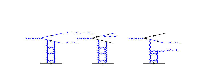
Figure 2: Diffractive dissociation of the virtual photon into quark - antiquark pair ( $q\bar{q}$ ) and quark - antiquark pair plus one extra gluon ( $q\bar{q}G$) in pQCD.

The paper is organized as follows. In section 2 we give a simple derivation of the Kovchegov and McLerran formula based on the $s$-channel unitarity constraints. We generalize this formula for the case of $q\bar{q}G$ final state ( see Fig.2 ) and discuss the relation between this approach and the AGK cutting rules [11]. Section 3 is devoted to a numeric calculation of the ratio $\sigma^{DD}/\sigma_{tot}$ without any restriction on the value of produced masses. In section 4 we discuss how limitations on the mass range change the energy dependence of the ratio. A summary of our results as well as a discussion on future HERA experiments are given in section 5. Appendix fives all formulae and all details of our calculations.

2 Shadowing corrections in QCD

2.1 Notations and definitions

In this paper we develop further our approach for diffractive production in DIS started in Ref.[7]. We use the same notations and definitions as in Ref. [7]. In this paper we examine the main physical ideas of Ref. [12], i.e. that the correct degrees of freedom at high enegies ( low $x$ ) are colour dipoles, rather than quarks and gluons which appear explicitly in the QCD Lagrangian. The consequence of this hypothesis is that a QCD interaction at high energies does not change the size and energy of a colour dipole. Hence, the majority of our variables and observables are related to the distribution and interaction of the colour dipoles in a hadron.

To facilitate reading the paper we list the notation and definitions which we will use ( see Fig.3 ):

Figure 3: Diffractive production of a quark - antiquark pair.

1. $Q^{2}$ denotes the virtuality of the photon in DIS, $M$ the produced mass and $W$ the energy of the collision in c.m. frame;

2. $x_{P}\,\,=\,\,(Q^{2}+M^{2})/W^{2}$ is the fraction of energy carried by the Pomeron ( two gluon ladder in Fig.3 ). Bjorken scaling variable is $x_{B}\,\,=\,\,Q^{2}/W^{2}$;

3. We use the symbol $x$ for both $x_{P}$ and $x_{B}$ .

4. $\beta\,\,=\,\,Q^{2}/(Q^{2}+M^{2})\,\,=\,\,x_{B}/x_{P}$ is the fraction of the Pomeron energy carried by the struck quark;

5. $k_{\perp}$ denotes the transverse momentum of the quark, and $r_{\perp}\,\,\equiv\,\,r$ the transverse distance between the quark and the antiquark i.e. the size of the colour dipole;

6. $l_{\perp}$ is the transverse momentum of the gluon emitted by the quark ( antiquark );

7. $z$ is the fraction of the photon momentum in the laboratory frame carried by the quark or antiquark;

8. $b_{t}$ is the impact parameter of the reaction and is the variable conjugated to $q_{\perp}$, the momentum transfer from the incoming proton to the recoiled proton. Note that $t=-q^{2}_{\perp}$;

9. Our amplitude is normalized so that

   $$\frac{d\sigma}{dt}\,\,=\,\,\pi\,|f(s=W^{2},t)|^{2}\,\,,$$ (2.1)

   with the optical theorem given by

   $$\sigma_{tot}\,\,\,=\,\,4\,\pi\,\,Im\,f(s,0)\,\,.$$ (2.2)

10. The scattering amplitude in $b_{t}$ space is defined by

    $$a^{el}(s,b_{t})\,\,=\,\,\frac{1}{2\,\pi}\,\int\,d^{2}\,q_{\perp}\,\,e^{-i\,\vec{\mathbf{q_{\perp}}}\cdot\vec{\mathbf{b_{t}}}}\,\,f(s,t=-q^{2}_{\perp})\,\,.$$ (2.3)

11. The $s$-channel unitarity constraint then has the form

    $$2\,Im\,a^{el}(s,b_{t})\,\,\,=\,\,\,|a^{el}(s,b_{t})|^{2}\,\,\,+\,\,\,G^{in}(s,b_{t})\,\,,$$ (2.4)

    where $G^{in}$ denotes the contribution of the all inelastic processes.

    Therefore, in the impact parameter representation:

    $$\sigma_{tot}\,\,\,=\,\,\,2\,\,\int\,\,d^{2}\,b_{t}\,\,Im\,a^{el}(s,b_{t})\,\,;$$ (2.5)

    $$\sigma_{el}\,\,\,=\,\,\,\int\,\,d^{2}\,b_{t}\,\,|\,a^{el}(s,b_{t})\,|^{2}\,\,;$$ (2.6)

    $$\sigma_{in}\,\,\,=\,\,\,\,\,\int\,\,d^{2}\,b_{t}\,\,G^{in}(s,b_{t})\,\,.$$ (2.7)

12. $x_{B}G(x_{B},Q^{2})$ is the gluon distribution of the nucleon;

13. $\sigma_{dipole}(x_{P},r_{\perp})$ is the total cross section for dipole - nucleon scattering, and is given by ( see Ref. [7] and references therein )

    $$\sigma_{dipole}(x_{P},r_{\perp})\,\,\,=\,\,\,\frac{\pi^{2}\alpha_{S}}{3}r^{2}_{\perp}\,\,x_{P}G(x_{P},\frac{4}{r^{2}_{\perp}})\,\,,$$ (2.8)

    where $x_{P}G(x_{P},\frac{4}{r^{2}_{\perp}})$ is the number of gluons with $Q^{2}=\frac{4}{r^{2}_{\perp}}$ and energy $x_{P}$ in the nucleon.

14. To characterize the strength of the colour dipole interaction we introduce

    $$\kappa_{dipole}\,\,\,=\,\,\frac{\sigma_{dipole}}{\pi R^{2}}\,\,=\,\,\frac{\pi^{2}\alpha_{S}}{3\,\pi\,R^{2}}r^{2}_{\perp}\,\,x_{P}G^{DGLAP}(x_{P},\frac{4}{r^{2}_{\perp}})\,\,,$$ (2.9)

    where $R$ is the nonperturbative parameter which is related to the correlation radius of the gluons in a hadron. We determine its value from high energy phenomenology and HERA experimental data ( see section 3 for discussion ).

    To illustrate the physical meaning of Eq. (2.9) we rewrite it in the form:

    $$\kappa_{dipole}\,\,\,=\,\,\sigma_{0}\,\,\rho(r_{\perp},x)\,\,,$$ (2.10)

    where

    $$\rho(r_{\perp},x)\,\,\,=\,\,\,\frac{xG^{DGLAP}(x,\frac{4}{r^{2}_{\perp}})}{\pi R^{2}}\,\,$$ (2.11)

    is the density of colour dipoles of size $r_{\perp}$ and energy $x$ in the transverse plane. In Eq. (2.10), $\sigma_{0}$ denotes the cross section for the interaction of a dipole of size $r_{\perp}$ with a point - like probe

    $$\sigma_{0}\,\,=\,\,\frac{\pi^{2}\alpha_{S}}{3}\,\,r^{2}_{\perp}\,\,.$$

    Hence, $\kappa_{dipole}$ is a packing factor for dipoles of size $r_{\perp}$ in a proton. If $\kappa_{dipole}$ is small, we have a diluted gas of colour dipoles in a proton, but at low $x$ the gluon density increases [10] and $\kappa_{dipole}\,\,\longrightarrow\,\,1$. In a such kinematic region our parton cascade becomes a dense system of colour dipoles which should be treated non-perturbatively;

15. The amplitude for colour dipole scattering on a nucleon is given by

    $$a^{el}_{dipole}(s,r_{\perp};b_{t})\,\,=\,\,\frac{\pi^{2}\alpha_{S}}{3}r^{2}_{\perp}\,\,x_{P}G(x_{P},\frac{4}{r^{2}_{\perp}};b_{t})\,\,,$$ (2.12)

    where $x_{P}G(x_{P},\frac{4}{r^{2}_{\perp}};b_{t})$ is the number of gluons at fixed impact parameter $b_{t}$.

16. It can be shown ( see Ref.[5] and references therein ) that we can write

    $$x_{P}G^{DGLAP}(x_{P},\frac{4}{r^{2}_{\perp}};b_{t})\,\,\,=\,\,\,x_{P}G^{DGLAP}(x_{P},\frac{4}{r_{\perp}})\,\,S(b_{t})\,\,,$$ (2.13)

    if $x_{P}G^{DGLAP}(x_{P},\frac{4}{r^{2}_{\perp}};b_{t})$ satisfies the DGLAP evolution equations[13].

    In Eq. (2.13) $S(b_{t})$ is the nucleon profile function which is a pure nonperturbative ingredient in our calculations. We assume a Gaussian form for

    $$S(b_{t})\,\,\,=\,\,\,\frac{1}{\pi\,R^{2}}\,\,e^{-\frac{b^{2}_{t}}{R^{2}}}\,\,,$$ (2.14)

    where $R$ has been discussed above;

17. For the exchange of one ladder ( “hard” Pomeron ) as shown in Fig. 3, $a^{el}_{dipole}$ can be written as

    $$\Omega^{P}_{dipole}\,\,=\,\,a^{el}_{dipole}(x,r_{\perp};b_{t})\,\,\,=\,\,\,\kappa^{DGLAP}_{dipole}(x,r_{\perp})\,\,e^{-\frac{b^{2}_{t}}{R^{2}}}\,\,$$ (2.15)

18. $\Psi^{\gamma^{*}}(z,r_{\perp};Q^{2})$ is the wave function of the quark - antiquark pair with the transverse distance $r_{\perp}$ between a quark and an antiquark and with a fraction of energy $z$ ( colour dipole of the size $r_{\perp}$ ). This wave function depends on the polarization of the virtual photon and it has been calculated previously in [8] [14].

    $$\Psi^{\gamma^{*}}_{L}(z,r_{\perp};Q^{2})\,\,\,=\,\,\,Q\,z\,(1-z)\,K_{0}(a\,r_{\perp})\,\,;$$ (2.16)

    $$\Psi^{\gamma^{*}}_{T}(z,r_{\perp};Q^{2})\,\,\,=\,\,\,i\,a\,K_{1}(a\,r_{\perp})\,\frac{\mathbf{\vec{r}_{\perp}}}{r_{\perp}}\,;$$ (2.17)

    where $a^{2}=z(1-z)Q^{2}+m^{2}_{q}$ and subscripts $T$ and $L$ denote the transverse and longitudinal polarizations of the photon, respectively.

19. In our calculations we only require the probabilty to find a quark-antiquark pair with the size $r_{\perp}$ inside a virtual photon, namely

    $$P^{\gamma^{*}}(z,r_{\perp};Q^{2}) = \frac{\alpha_{em}N_{c}}{2\pi^{2}}\,\sum_{f}\,Z^{2}_{f}\sum_{\lambda_{1},\lambda_{2}}\,\{\,|\Psi_{T}|^{2}\,\,+\,\,|\Psi_{L}|^{2}\,\}\,\,$$

    $$= \frac{\alpha_{em}N_{c}}{2\pi^{2}}\sum_{f}Z^{2}_{f}\,\{\,(z^{2}+(1-z)^{2})a^{2}K^{2}_{1}(a\,r_{\perp})\,+\,4\,Q^{2}\,z^{2}(1-z)^{2}K^{2}_{0}(a\,r_{\perp})\,\}.$$

2.2 Shadowing corrections for penetration of $\mathbf{q\bar{q}}$ pair through the target.

2.2.1 General approach

The physics underlying our approach has been formulated and developed in Refs. [15] [8]. During its passage through the target, the distance $r_{\perp}$ between a quark and an antiquark can vary by an amount $\Delta r_{\perp}\,\,\propto\,\,Rk_{\perp}/E$, where $E$ is the pair energy and $R$ is the size of the target. Since the quark’s transverse momentum $k_{\perp}\,\,\propto\,\,1/r_{\perp}$, the relation

$$\Delta\,r_{\perp}\,\,\propto\,\,R\,\frac{k_{\perp}}{E}\,\,\approx\,\,R\,\frac{1}{r_{\perp}\,\,E}\,\,\ll\,\,r_{\perp}$$ (2.19)

holds if

$$r^{2}\,s\,\,\gg\,\,2mR\,\,,$$ (2.20)

where $s=W^{2}=2mE$ with $m$ being the mass of the hadron.

Eq. (2.20) can be rewritten in terms of $x_{P}$, namely,

$$x_{P}\,\,\ll\,\,\frac{2}{(1-\beta)mR}\,\,.$$ (2.21)

From Eq. (2.21) it follows that $r_{\perp}$ is a good degree of freedom [8] for high energy scattering.

We can therefore write the total cross section for the interaction of the virtual photon with the target as follows:

$$\sigma_{tot}(\gamma^{*}+p)\,\, = \,\,\int\,dz\,\int\,d^{2}\,r_{\perp}\,P^{\gamma^{*}}(z,r_{\perp};Q^{2})\,\,\sigma_{dipole}(x_{B},r_{\perp})\,\,$$ (2.22)

$$= 2\,\int\,d^{2}b_{t}\,\,\int dz\,\int\,d^{2}\,r_{\perp}\,\,P^{\gamma^{*}}(z,r_{\perp};Q^{2})\,\,Im\,a^{el}_{dipole}(x_{B},r_{\perp};b_{t})\,\,.$$ (2.23)

The amplitude for diffractive production of a $q\bar{q}$ - pair is equal to

$$a^{DD}(\gamma^{*}+p\,\rightarrow\,q+\bar{q})\,\,=\,\,\int d^{2}\,r_{\perp}\,\,\Psi^{\gamma^{*}}(z,r_{\perp};Q^{2})\,a^{el}_{dipole}(x_{B},r_{\perp};b_{t})\,\,\Psi^{q\bar{q}}(k_{\perp},z,r_{\perp})\,\,,$$ (2.24)

where $\Psi^{q\bar{q}}(k_{\perp},z,r_{\perp})$ is the wave function of the quark-antiquark pair with fixed momentum $k_{\perp}$ and fraction of energy $z$. To calculate the total cross section of the diffractive production we should integrate over all $k_{\perp}$ and $z$. Using the completeness of the $q\bar{q}$ wave function one obtains

$$\sigma^{DD}(\gamma^{*}+p\,\rightarrow\,q+\bar{q})\,\,\,=\,\,\int\,d^{2}\,b_{t}\,\,\int dz\,\int\,d^{2}\,r_{\perp}\,P^{\gamma^{*}}(z,r_{\perp};Q^{2})\,|a^{el}_{dipole}(x_{B},r_{\perp};b_{t})|^{2}\,\,.$$ (2.25)

Utilizing the unitarity constraint we obtain a prediction for the ratio

$${\Re}\,\,=\,\,\frac{\sigma^{DD}}{\sigma_{tot}}\,\,=\,\,\frac{\int\,d^{2}\,b_{t}\,\int\,dz\,\int\,d^{2}\,r_{\perp}\,\,P^{\gamma^{*}}(z,r_{\perp};Q^{2})\,|a^{el}_{dipole}(x_{B},r_{\perp};b_{t})|^{2}}{2\,\int\,d^{2}b_{t}\,\int\,dz\,\int\,d^{2}\,r_{\perp}\,\,P^{\gamma^{*}}((z,r_{\perp};Q^{2})\,\,Im\,a^{el}_{dipole}(x_{B},r_{\perp};b_{t})}\,\,.$$ (2.26)

Eq. (2.26) is a general prediction for the ratio $\Re$ [16][3]. It shows that the diffractive dissociation and total cross sections are related through unitarity. However, Eq. (2.26) is too general to be used for pratical estimates.

Assuming that the dipole - proton amplitude is mainly imaginary at high energy the unitarity constraint of Eq. (2.4) has a general solution

$$a^{el}_{dipole}(x,r_{\perp};b_{t})\,\,=\,\,i\,\left(\,1\,\,-\,\,e^{-\frac{\Omega(x,r_{\perp};b_{t})}{2}}\,\right)\,\,;$$ (2.27)

$$G^{in}_{dipole}(x,r_{\perp};b_{t})\,\,=\,\,1\,\,-\,\,e^{-\Omega(x,r_{\perp};b_{t})}\,\,;$$ (2.28)

where $\Omega$ is arbitrary real function.

Using Eq. (2.27) and Eq. (2.28), Eq. (2.26) reduces to

$$\Re\,\,=\,\,\frac{\sigma^{DD}}{\sigma_{tot}}\,\,=\,\,\frac{\int\,d^{2}\,b_{t}\int\,dz\int\,d^{2}r_{\perp}P^{\gamma^{*}}(z,r_{\perp};Q^{2})\,\left(\,1\,\,-\,\,e^{-\frac{\Omega(x,r_{\perp};b_{t})}{2}}\,\right)^{2}}{2\,\int\,d^{2}b_{t}\,\int\,dz\,\int\,d^{2}\,r_{\perp}\,\,P^{\gamma^{*}}(z,r_{\perp};Q^{2})\,\,\left(\,1\,\,-\,\,e^{-\frac{\Omega(x,r_{\perp};b_{t})}{2}}\,\right)}\,\,.$$ (2.29)

The main goal of our microscopic approach based on QCD is to find $\Omega$ .

2.2.2 Mueller-Glauber approach

One way to get a more detailed picture of the interaction, is to consider the dipole - proton interaction in the Eikonal model, which is closely related to Mueller - Glauber approach [8].

The main assumption of this model is to identify the function $\Omega$ in Eq. (2.29) with the exchange of the “hard” Pomeron ( gluon ladder ) given by Eq. (2.15) ( see Fig. 3 ). Since the gluon distribution given by the DGLAP evolution equations originates from inelastic processes of gluon emission, we assume an oversimplified structure of the final states in the Eikonal model, namely, it consists of only a proton and a quark-antiquark pair ( “elastic” scattering ), and an inelastic state with a large number of emitted gluons ($N_{G}\,\,\propto\,\,\ln(1/x)$ . In particular, we neglect the rich structure of the diffraction dissociation processes and simplify them to the final state of $p+q\bar{q}$. For example, we neglect the diffractive production of an excited nucleon in DIS.

We will discuss the accuracy of our approach in the next subsection, where we expand our model to include an excitation of the target. Our accuracy is restricted by the assumption of only a quark - antiquark pair and a nucleon in the final state for diffractive processes. The rough estimate for the contribution of all excitations of the nucleon is

$$\frac{\sigma^{DD}(\gamma^{*}+p\,\rightarrow\,\,q\bar{q}+N^{*})}{\sigma^{DD}(\gamma^{*}+p\,\rightarrow\,\,q\bar{q}+N)}\,\,\,=\,\,\sqrt{\frac{\sigma^{DD}(p+p\,\rightarrow\,\,p+N^{*})}{2\,\,\sigma_{el}(p+p\,\rightarrow\,\,p+p)}}\,\,\approx\,\,0.2\div 0.3\,\,.$$ (2.30)

consequently, we have to consider the nucleon excitations or, at least, to discuss them in the HERA kinematic region.

Substituting $\Omega=\Omega^{P}$ ( see Eq. (2.15) ) in Eq. (2.29) we obtain the Kovchegov - McLerran formula [8] [17], then for large $Q^{2}$ we have

$$\int^{1}_{0}\,dz\,\,P_{T}^{\gamma^{*}}(z,r_{\perp};Q^{2})\,\,=\,\,\frac{4\,\alpha_{em}N_{c}}{3\,\pi^{2}\,Q^{2}}\,\times\,\frac{1}{r^{4}_{t}}\,\,.$$ (2.31)

We can see from Eq. (2.29) and Eq. (2.31) that

$$\sigma^{DD}\,\propto\,\,R^{2}Q^{2}/<r^{2}_{\perp}>\,\,;$$

$$\sigma_{tot}\,\propto\,\,R^{2}Q^{2}/<r^{2}_{\perp}>\,\,;$$

we can evaluate $<r^{2}_{\perp}>$ from the condition

$$\Omega^{P}_{dipole}(b_{t}=0)\,\,\,=\,\,\,\kappa^{DGLAP}_{dipole}(x,<r_{\perp}>)\,\,=\,\,1\,\,.$$ (2.32)

If we assume that $xG(x,\frac{4}{r^{2}_{\perp}})$ depends rather smoothly on $r^{2}_{\perp}$, and substitute $\frac{4}{r^{2}_{\perp}}=Q^{2}$ as an estimate, we have

$$\frac{1}{<r_{\perp}>}\,\,\propto\,\,xG(x,Q^{2})\,\,.$$ (2.33)

Eq. (2.33) gives the ratio $\Re$ constant as well as $\sigma^{DD}\,\propto\,\,R^{2}Q^{2}\,\times\,x_{B}G(x_{B},Q^{2})$. This simple estimate, given in Ref. [3], illustrates that the SC lead to a constant ratio $\Re$, or, vice versa, the constant ratio $\Re$ can be a strong argument for substantial SC. To examine this point we calculate the ratio $\Re$ using the same assumption that $\frac{4}{r^{2}_{\perp}}=Q^{2}$ in the gluon distribution. Using the result of the explicit calculation in Ref.[18] we obtain:

$$\Re\,\,=\,\,\frac{\sigma^{DD}}{\sigma_{tot}}\,\,=\,\,1\,\,-\,\,\frac{\ln(\kappa_{dipole})\,\,+\,\,C\,\,+\,\,(\,1\,+\,\kappa_{dipole}\,)\,E_{1}(\kappa_{dipole})\,+\,1\,-\,e^{-\kappa_{dipole}}}{2\,[\ln(\frac{\kappa_{dipole}}{2})\,\,+\,\,C\,\,+\,\,(\,1\,+\,\frac{\kappa_{dipole}}{2}\,)\,E_{1}(\,\frac{\kappa_{dipole}}{2})\,+\,1\,-\,e^{-\frac{\kappa_{dipole}}{2}}\,]}\,\,.$$ (2.34)

Fig. 4-a	Fig. 4-b

Figure 4: Ratio $\sigma^{DD}/\sigma_{tot}$ calculated using Eq. (2.34) in the Eikonal model for $q\bar{q}$ diffractive production.

In Fig.4 the ratio $\Re$, given by Eq. (2.34), is plotted as a function of $\kappa_{dipole}$. One can see that at large $\kappa_{dipole}$ this ratio has a smooth dependence on $\kappa_{dipole}$. However, the values of $\kappa_{dipole}$ that we are dealing with are not very large ( $\kappa_{dipole}\,\,\approx\,\,1$, see Fig.5, where $\kappa_{dipole}$ is calculated using the GRV parameterization for the gluon distribution [19] ). Fig.4-a shows that for $\kappa_{dipole}=0.2-2$ we cannot expect that Eq. (2.34) to yield a more or less constant ratio $\Re$.

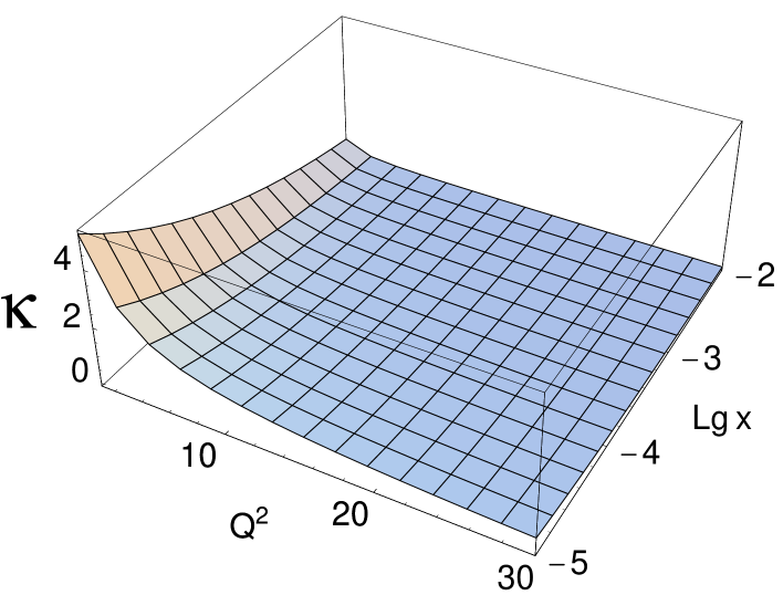
Figure 5: $\kappa_{dipole}$ calculated in HERA kinematic region, using the GRV-94 parameterization [19] for the gluon distrubution. $lgx=log_{10}(x)$.

However, we would like to draw the reader’s attention to the fact that the ratio differs from the small $\kappa_{dipole}\,\,\ll\,\,1$ limit where $\Re\,\,\propto\,\,\kappa_{dipole}$.

These simple estimates indicate that the SC are essential, but they are still not sufficiently strong to use the asymptotic formulae. We are in the transition region from low density QCD, described by the DGLAP evolution, to high density QCD where we can use the quasi-classical gluon field approximation [20]. In the transition region the Mueller-Glauber approach is a natural way to obtain reliable estimates of the SC. However, we need to study corrections to Eq. (2.29) more carefully. The most important among them, are the diffractive production of nucleon excitation ( see Eq. (2.30)) and of the $q\bar{g}G$ system, which gives the dominant contribution to the diffractive cross section [7].

2.2.3 Diffractive production of nucleon excitations

A. General approach

We start with a trivial remark, that the nucleon excitations even in DIS are closely related to long distance processes and, therefore, to the “soft” interaction which cannot be determined in QCD. An alternate way of saying this is, to attribute these diffractive processes to nonperturbative QCD, for which at present we only have a phenomenological approach. Theoretically “soft” diffraction can be viewed [21] as a typical quantum mechanical process which occurs, since the hadron states are not diagonal with respect to the strong interaction scattering matrix. In other words diffractive dissociation occurs, because even at high energy hadrons are not the correct degrees of freedom for the strong nonperturbative interaction. Unfortunately, we do not know the correct degrees of freedom and below we will discuss some models for them. We denote by $n$ the correct degree of freedom or the set of quantum numbers which characterizes the wave function $\Psi_{n}$. These function $\Psi_{n}$ are diagonal with respect to the strong interaction

$$A_{n,n^{\prime}}\,\,=\,\,\big{<}\Psi_{n}\big{|}{\mathbf{T}}\big{|}\Psi_{n^{\prime}}\big{>}\,\,=\,\,A_{n}\,\,\delta_{n,n^{\prime}}\,\,,$$ (2.35)

where parentheses denote all needed integrations and $\mathbf{T}$ is the scattering matrix.

Note, that only for amplitudes $A_{n}$ do we have the unitarity constraints in the form of Eq. (2.4), namely,

$$Im\,A^{el}_{n}(s,b_{t})\,\,\,=\,\,|A^{el}_{n}(s,b_{t})|^{2}\,\,\,+\,\,\,G^{in}_{n}(s,b_{t})$$ (2.36)

which has solutions of Eq. (2.27) and Eq. (2.28) for mainly imaginary $A_{n}$ at high energies:

$$A^{el}_{n}\,\,\,=\,\,i\,\{\,\,1\,\,\,-\,\,\,e^{-\frac{\Omega_{n}(s,b_{t})}{2}}\,\,\}\,\,;$$ (2.37)

$$G^{in}_{n}\,\,\,=\,\,\,1\,\,\,-\,\,\,e^{-\Omega_{n}(s,b_{t})}\,\,.$$ (2.38)

The wave function of a hadron is

$$\Psi_{hadron}\,\,=\,\,\sum^{\infty}_{n=1}\,\,\alpha_{n}\,\,\Psi_{n}\,\,.$$ (2.39)

For a dipole - hadron interaction the wave function is equal to $\Psi_{dipole}(r_{\perp})\,\times\,\Psi_{hadron}$ before collision. After collision the scattering matrix $\mathbf{T}$ leads to a new wave function,namely

$$\Psi_{final}\,\,=\,\,\Psi_{dipole}(r_{\perp})\,\times\,\sum^{\infty}_{n=1}\,\,\alpha_{n}\,\,A_{n}\,\Psi_{n}\,\,.$$ (2.40)

From Eq. (2.40) we obtain the elastic amplitude

$$a^{el}_{dipole}\,\,=\,\,\big{<}\Psi_{final}\big{|}\Psi_{dipole}(r_{\perp})\,\times\,\Psi_{hadron}\big{>}\,\,=\,\,\sum^{\infty}_{n=1}\,\,\alpha^{2}_{n}\,A_{n}(s,b_{t})\,\,\,,$$ (2.41)

while for the total cross section of the diffractive nucleon excitations we have

$$\sigma^{DD}_{N^{*}}\,\, = \,\,\big{<}\Psi_{final}\big{|}\Psi_{final}\big{>}^{2}\,\,\,-\,\,\big{<}\Psi_{final}\big{|}\Psi_{dipole}(r_{\perp})\,\times\,\Psi_{hadron}\big{>}^{2}\,\,;$$ (2.42)

$$= \,\,\sum^{\infty}_{n=1}\,\,\alpha^{2}_{n}\,|A_{n}(s,b_{t})|^{2}\,\,\,-\,\,\{\,\sum^{\infty}_{n=1}\,\,\alpha^{2}_{n}\,A_{n}(s,b_{t})\,\}^{2}\,\,.$$ (2.43)

Therefore, using Eq. (2.31) instead of Eq. (2.29), we obtain a generalized formula

$$\Re\,\,=\,\,\frac{\sigma^{DD}}{\sigma_{tot}}\,\,\,=\,\,\,\frac{\sum^{\infty}_{n=1}\,\alpha^{2}_{n}\,\,\int\,d^{2}\,b_{t}\int\,\frac{dr^{2}_{\perp}}{r^{4}_{\perp}}\,\{\,1\,\,-\,\,e^{-\frac{\Omega^{P}_{n}(r^{2}_{\perp},y;b_{t})}{2}}\,\}^{2}}{2\,\,\sum^{\infty}_{n=1}\,\alpha^{2}_{n}\,\,\int\,d^{2}\,b_{t}\int\,\frac{dr^{2}_{\perp}}{r^{4}_{\perp}}\,\{\,1\,\,-\,\,e^{-\frac{\Omega^{P}_{n}(r^{2}_{\perp},y;b_{t})}{2}}\,\}}\,\,,$$ (2.44)

One can see that this generalized formula has all the attractive features of Eq. (2.29), and at small $x$ the ratio tends to $1/2$, since the normalization constraint

$$\sum^{\infty}_{n=1}\,\,\alpha^{2}_{n}\,\,=\,\,1$$ (2.45)

We can estimate $\Omega^{P}_{n}$ using the same Eq. (2.15) here

$$\Omega_{n}\,\,=\,\,\kappa^{n}_{dipole}\,\,\,e^{-\frac{b^{2}_{t}}{R^{2}_{n}}}\,\,,$$ (2.46)

where

$$\kappa^{n}_{dipole}\,\,\,=\,\,\,\frac{\pi^{2}\alpha_{S}}{3\,\pi\,R^{2}_{n}}r^{2}_{\perp}\,\,x_{P}G_{n}(x_{P},\frac{4}{r^{2}_{\perp}})\,\,.$$ (2.47)

Therefore, the main difficulty with Eq. (2.46) and Eq. (2.47) is to determine $R_{n}$ and $xG_{n}(x,\frac{4}{r^{2}_{\perp}})$. We only have direct experimental information for the proton radius and the gluon distribution in the proton. Unfortunately, we cannot evaluate Eq. (2.44) without developing some model for the diffractive excitations.

B. Two channel model for diffractive nucleon excitations.

The main idea [22] of this model is to replace the many final states of diffractively produced hadrons by one state ( effective hadron ). In this case the general Eq. (2.39) reduces to the simple form

$$\Psi_{hadron}\,\,\,=\,\,\alpha_{1}\,\,\Psi_{1}\,\,\,+\,\,\,\alpha_{2}\,\,\Psi_{2}\,\,,$$ (2.48)

with the condition $\alpha^{2}_{1}\,\,+\,\,\alpha^{2}_{2}\,\,=\,\,1$ from Eq. (2.45).

The wave function of the produced effective hadron is equal to

$$\Psi_{D}\,\,\,=\,\,-\,\alpha_{2}\,\,\Psi_{1}\,\,\,+\,\,\,\alpha_{1}\,\,\Psi_{2}\,,$$ (2.49)

which is orthogonal to $\Psi_{hadron}$.

Eq. (2.44) can be rewritten in the form

$$\Re\,\, = \,\,\frac{\sigma^{DD}}{\sigma_{tot}}\,\,\,=\,\,\$$

$$= \,\,\,\frac{\,\,\,\int\,d^{2}\,b_{t}\int\,\frac{dr^{2}_{\perp}}{r^{4}_{\perp}}\,\left(\,\alpha^{2}_{1}\{\,1\,\,-\,\,e^{-\frac{\Omega^{P}_{1}(r^{2}_{\perp},y;b_{t})}{2}}\,\}^{2}\,\,+\,\,\alpha^{2}_{2}\,\,\{\,1\,\,-\,\,e^{-\frac{\Omega^{P}_{2}(r^{2}_{\perp},y;b_{t})}{2}}\,\}^{2}\,\right)}{2\,\,\int\,d^{2}\,b_{t}\int\,\frac{dr^{2}_{\perp}}{r^{4}_{\perp}}\,\left(\,\{\,1\,\,-\,\,e^{-\frac{\Omega^{P}_{1}(r^{2}_{\perp},y;b_{t})}{2}}\,\}\,\,+\,\,\alpha^{2}_{2}\,\,e^{-\frac{\Omega^{P}_{1}(r^{2}_{\perp},y;b_{t})}{2}}\,\{\,1\,\,-\,\,e^{-\frac{\Delta\Omega^{P}(r^{2}_{\perp},y;b_{t})}{2}}\,\}\,\right)}\,\,;$$

with $\Delta\Omega\,\,=\,\,\Omega_{2}\,-\,\Omega_{1}$.

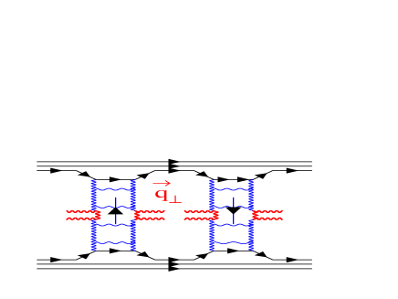
Fig. 6-a	Fig. 6-b

Figure 6: Mueller diagrams [24] for J/$\Psi$ photoproduction ( Fig.6-a ) and for double parton interaction ( Fig.6-b ).

For $\Omega_{1}$ and $\Delta\Omega$ we use the parameterization given by Eq. (2.46) and Eq. (2.47), and the following experimental data and phenomenological observations:

1. Data for single diffraction in proton - proton collisions lead to $\alpha^{2}_{2}\,\,\approx\,\,0.2$ Ref. [22]  ;

2. Data for J/$\Psi$ photoproduction at HERA [23] ( see Fig.6a ) show that $t$-dependance is quite different for elastic and inelastic photoproduction. The measured values are $B_{el}\,\,=\,\,4\,\,GeV^{-2}$ while $B_{in}\,\,=\,\,1.66\,\,GeV^{-2}$. Therefore, we take $R^{2}_{1}=2\,B_{el}=8\,\,GeV^{-2}$ in $\Omega_{1}$ and $R^{2}_{D}=2B_{in}=3.32\,\,GeV^{-2}$, where $R^{2}_{D}$ is the radius in the exponential parameterization for $\Delta\Omega$ ;

3. The energy behaviour of diffractive J/$\Psi$ photoproduction shows that we can consider this process as a typical “hard” process which occurs at short distances [10] ;

4. We use experimental evidence [23] that the cross section for elastic and inelastic diffractive J/$\Psi$ photoproduction are equal. From this fact we can conclude that

   $$\alpha_{2}\,(1-\alpha_{2})(\Delta\Omega)(b_{t}=0)^{2}\,\,R^{2}_{D}\,\,=\,\,(1-\alpha_{2})^{2}\,\Omega^{2}_{1}(b_{t}=0)\,\,R^{2}_{1}\,\,,$$ (2.51)

   which gives

   $$\Delta\Omega(b_{t}=0)\,\,=\,\,\sqrt{\frac{(1-\alpha^{2}_{2})}{\alpha^{2}_{2}}}\,\frac{R_{1}}{R_{D}}\,\,\Omega_{1}(b_{t}=0)\,\,.$$ (2.52)

   Substituting in Eq. (2.52) we find $\Delta\kappa_{dipole}\,\,\approx\,\,3.4\,\,\kappa^{1}_{dipole}$.

Fig. 7-a	Fig. 7-b

Figure 7: Ratio $\sigma^{DD}/\sigma_{tot}$ (Fig.7a) and ratio $\sigma^{DD}_{excitation}/\sigma^{DD}_{elastic}$ (Fig. 7b) versus $\kappa_{dipole}$ calculated in two channel model for nucleon excitations for $q\bar{q}$ diffractive production.

In Fig. 7 we display the ratio $R$ as a function of $\kappa_{dipole}$. Comparing this figure with Fig. 4a we can conclude that in the two channel model, R increases more or less at the same rate as in the Eikonal model, but the value of the ratio depends crucially on the model for the diffractive excitation of the nucleon. Fig. 7b shows the contamination of the total diffractive cross section by the nucleon excitations. One can conclude that the two channel model gives a small fraction of the excitation cross section at sufficiently large $\kappa_{dipole}$. Experimentally,$\sigma^{DD}_{excitation}/\sigma^{DD}_{elastic}$ = $35\,\pm\,15\%$. Fig.7b supports a low value for this ratio, but this question should be reconsidered after taking into account the diffractive production of the $q\bar{q}G$ system.

C. Diffractive production in the Additive Quark Model

As we have mentioned, the main problem of dealing with the “soft” high energy interaction, is to find the correct degrees of freedom, and to incorporate them in the general formalism for high energy scattering. The two channel model gives an estimate of the importance of proton excitation processes, but it is too phenomenological to be instructive and not totally reliable. Here, we consider the nucleon excitation in the Additive Quark Model [25]. In this model the correct degrees of freedom at high energies are the constituent quarks. In spite of a certain naivity this model has not been abandoned and it is included in the standard Donnachie - Landshoff Pomeron approach[26] for “soft” processes at high energies.

Inherent in this model is the assumption, that the $\gamma^{*}$ - constituent quark interactions dominate, while other interactions e.g. the interaction of $\gamma^{*}$ with two constituent quarks, are suppressed by factor $r^{2}_{Q}/R^{2}_{N}$ , here $r_{Q}$ is the size of the constituent quark and $R_{N}$ is the radius of the proton. It is obvious that in the AQM we have the same Eq. (2.29) ( or Eq. (2.26) ) where $\Omega=\Omega^{P}_{Q}$ describes the interaction of a colour dipole with the constituent quark. In the AQM the gluon distribution of the constituent quark is equal to $xG_{Q}(x,Q^{2})\,=\,\frac{1}{3}\,xG_{N}(x,Q^{2})$ and, therefore

$$\Omega^{P}_{Q}(x,r_{\perp};b_{t})\,\,\,=\,\,\kappa^{Q}_{dipole}\,\,e^{-\frac{b^{2}_{t}}{r^{2}_{Q}}}\,\,=\,\,\frac{\pi^{2}\alpha_{S}}{9\,\pi\,r^{2}_{Q}}r^{2}_{\perp}\,\,xG_{N}(x,\frac{4}{r^{2}_{\perp}})\,\,e^{-\frac{b^{2}_{t}}{r^{2}_{Q}}}\,\,.$$ (2.53)

Consequently, we find $r_{Q}$ using the same AQM to describe the double parton cross section measured by the CDF [27] (see Fig. 7b ). The CDF collaboration has measured the inclusive cross section for the production of two “hard” pairs of jets, with large and almost compensating transverse momenta in each pair, and with similar values of rapidity. Such processes cannot occur in a one parton shower, and only originate from two parton shower interactions as shown in Fig.7b.

The double parton cross section can be written in the form [27]

$$\sigma_{DP}\,\,=\,\,m\,\frac{\sigma_{inel}(2jets)\,\,\sigma_{inel}(2jets)}{2\sigma_{eff}}\,\,$$ (2.54)

where factor $m$ is equal to 2 for different pairs of jets, and to 1 for identical pairs. The experimental value[27] of $\sigma_{eff}\,\,=\,\,14.5\,\,\pm\,\,1.7\,\,\pm\,\,2.3\,\,mb$.

In the AQM (see Fig.7b ) $\sigma_{eff}$ can be easily calculated and it is equal to

$$\sigma_{eff}\,\,=\,\,9\,\times\,2\pi\,r^{2}_{Q}\,\,,$$ (2.55)

where factor 9 reflects the quark counting and $2\pi r^{2}_{Q}$ comes from the integration over $b_{t}$. Comparing Eq. (2.55) with the experimental value of $\sigma_{eff}$ we obtain $r^{2}_{Q}\,\,=\,\,0.66\,\pm\,0.16\,GeV^{-2}$.

Substituting this result in Eq. (2.53) we find $\kappa^{Q}_{dipole}\,\,\approx\,\,5\,\kappa^{N}_{dipole}$ with the same $x$ and $r_{\perp}$ dependance. In Fig. 8 one can see the prediction for the ratio $\sigma^{DD}/\sigma_{tot}$. This approach gives the ratio which depends smoothly on $\kappa_{dipole}$ for $\kappa_{dipole}\,>\,0.75$.

Comparing Fig.8 and Fig.4a we can conclude that the diffractive production of the nucleon excitations gives about 30% of the total diffractive cross section at $\kappa_{dipole}\,\approx\,0.2-0.6$ and becomes very small at $\kappa_{dipole}\,\approx\,1.5-2$.

Fig. 8-a	Fig. 8-b

Figure 8: Ratio $\sigma^{DD}/\sigma_{tot}$ (Fig.8a) and ratio $\sigma^{DD}_{excitation}/\sigma^{DD}_{elastic}$ (Fig. 8b) versus $\kappa_{dipole}$ calculated in the Additive Quark Model for nucleon excitations for $q\bar{q}$ diffractive production.

2.2.4 AGK cutting rules and diffractive production

In this section we derive Eq. (2.29) in the Mueller-Glauber approach exploiting the AGK cutting rules [11]. This derivation is more complicated than the previous derivation which was based directly on the $s$-channel unitarity constraints. As we intend using the AGK cutting rules for calculating the diffraction production of the $q\bar{q}G$ system, we think it instructive to start with a simple example.

The AGK cutting rules provide a prescription of how to calculate the cross sections for the processes with different multiplicities of the produced particles, if one knows the structure of the Pomeron exchange, and the expression for the total cross section in terms of multi Pomeron exchanges [11] [28]. In the Mueller-Glauber approach we have such an expression for the total colour dipole - proton cross section, namely, (see Fig.9)

$$\sigma_{dipole}\,\,\,=\,\,2\,\int\,d^{2}b_{t}\,\,\{\,1\,\,-\,\,e^{-\frac{\Omega^{P}(x,r_{\perp};b_{t})}{2}}\,\}\,\,,$$ (2.56)

where $\Omega^{P}$ is given by Eq. (2.15). We first need to define the Pomeron structure i.e. to specify the kind of inelastic processes that are described by $\Omega^{P}$. From Eq. (2.15) we see that $\Omega^{P}$ describes the inelastic processes with large average multiplicity ( $<n_{P}>$ ) of produced partons, since it is related to the DGLAP parton cascade. For example, at large $Q^{2}$ and low $x$, $<n_{P}>\,\,=\,\,2\sqrt{\bar{\alpha}_{S}\ln Q^{2}\ln(1/x)}\,\,\gg\,\,1$. The AGK cutting rules allow us to calculate the cross sections for the processes with average multiplicities 2$<n_{P}>$, 3 $<n_{P}>$ and so on, as well as the process for the diffractive dissociation with multiplicity much smaller that $<n_{P}>$.

Eq. (2.56) can be rewritten in the form

$$\sigma_{dipole}\,\,\,=\,\,2\,\int\,d^{2}b_{t}\,\,\sum^{\infty}_{n=1}\,\,C_{n}\,(-1)^{n+1}\,\,\left(\,\frac{\Omega^{P}}{2}\,\right)^{n}\,\,,$$ (2.57)

where each term corresponds to the exchange of $n$ Pomerons. The AGK rules are

$$\sigma^{n}_{dipole}(k<n_{P}>)\, = \,\int\,d^{2}b_{t}\,C_{n}(-1)^{n-k}\,\frac{n!}{(n-k)!\,k!}\,\,\left(\,\Omega^{P}\,\right)^{n}\,\,\,;$$ (2.58)

$$\sigma_{dipole}^{n}(DD)\, = \,\int\,d^{2}b_{t}\,C_{n}(-1)^{n}\,\{\,\left(\,\Omega^{P}\,\right)^{n}\,\,-\,\,2\,\left(\,\frac{\Omega^{P}}{2}\,\right)^{n}\,\}\,\,;$$ (2.59)

where $\sigma^{n}_{dipole}(k<n_{P}>)$ and $\sigma_{dipole}^{n}(DD)$ are the contributions of $n$-Pomeron exchange to the cross section for the process with average multiplicity $k<n_{P}>$, and to the cross section for the diffractive dissociation processes with small multiplicity.

Figure 9: Total cross section for the dipole - nucleon interaction in the Mueller-Glauber approach. The dashed line shows the diffraction dissociation cut.

Summing over $n$ in Eq. (2.59) we obtain

$$\sigma^{DD}_{dipole}(r_{\perp})\,\, = \,\,\int\,d^{2}b_{t}\,\sum^{\infty}_{n=1}\,\,C_{n}\,(-1)^{n}\,\{\,\left(\,\Omega^{P}\,\right)^{n}\,\,-\,\,2\,\left(\,\frac{\Omega^{P}}{2}\,\right)^{n}\,\}\,\,;$$ (2.60)

$$= \,\,\int\,d^{2}b_{t}\,\left(\,2\,\{\,1\,\,-\,\,e^{-\frac{\Omega^{P}}{2}}\,\}\,\,-\,\,\{\,1\,\,-\,\,e^{-\Omega^{P}}\,\}\,\right)\,\,;$$ (2.61)

$$= \,\,\int\,d^{2}b_{t}\,\left(\,1\,\,-\,\,e^{-\frac{\Omega^{P}}{2}}\,\right)^{2}\,\,.$$ (2.62)

One can see that Eq. (2.62) is just the same equation for diffractive production that we have obtained from unitarity ( see Eq. (2.29) ). From Eq. (2.58) we can find the cross section for the production of $k$ - parton showers which is equal to

$$\sigma_{dipole}(k<n_{P}>)\,\,\,=\,\,\int\,\,d^{2}\,b_{t}\,\,\,\frac{\left(\,\Omega^{P}\,\right)^{k}}{k!}\,\,e^{-\Omega^{P}}\,\,.$$ (2.63)

Eq. (2.63) will be very useful below, when we discuss the diffraction production of the $q\bar{q}G$ system.

2.3 Cross section for $\mathbf{q\bar{q}G}$ diffractive production with SC

2.3.1 First correction to the Mueller - Glauber formula for the total cross section

As shown in Fig.9, the Eikonal approach takes into account only rescatterings of the fastest colour dipole. In this subsection we will extend the formalism so as also to include the rescatterings with the target of the two fastest color dipoles: the initial colour dipole and the fastest gluon in Fig.9. Our goal is to include all diagrams of the type shown in Fig.10. Dashed lines in Fig.10 indicate the diffraction dissociation cuts. These diagrams include the diffractive production of $q\bar{q}G$ system as well as a quark - antiquark pair.

Since Eq. (2.27) and Eq. (2.28) give the general solution to the unitarity constraint, our problem is to find an expression for $\Omega$ which will be more general that Eq. (2.15) with $\kappa^{DGLAP}$ defined by Eq. (2.9).

Figure 10: Total cross section for dipole - nucleon interaction in the first iteraction of the Mueller-Glauber approach. The dashed lines show the diffraction dissociation cut.

The natural generalization of $\kappa^{DGLAP}$ is to substitute in Eq. (2.9) the Mueller-Glauber formula for the gluon structure function [8] [18], namely

$$\frac{1}{\pi R^{2}}\,\,xG^{DGLAP}(x,\frac{4}{r^{2}_{\perp}})\,\,e^{-\frac{b^{2}_{t}}{R^{2}}}\,\,\longrightarrow\,\,xG^{MG}(x,\frac{4}{r^{2}_{\perp}};b_{t})\,\,\,=\,\,$$ (2.64)

$$\frac{4}{\pi^{3}}\,\,\int^{1}_{x}\,\frac{dx^{\prime}}{x^{\prime}}\int^{\infty}_{r^{2}_{\perp}}\,\,\frac{d\,r^{\prime 2}_{\perp}}{r^{\prime 4}_{\perp}}\,2\,\{\,1\,\,\,-\,\,e^{-\frac{\Omega^{P}_{G}(x^{\prime},r^{\prime}_{\perp};b_{t})}{2}}\,\}\,\,,$$

where

$$\Omega^{P}_{G}\,\,=\,\,\frac{3\pi^{2}\alpha_{S}}{4\pi R^{2}}\,\,r^{2}_{\perp}\,\,G^{DGLAP}(x,\frac{4}{r^{2}_{\perp}})\,\,e^{-\frac{b^{2}_{t}}{R^{2}}}\,\,.$$ (2.65)

Eq. (2.64) takes into account the rescattering of the gluon with the target in the Eikonal approach ( see Fig.10), however, the question arises of why we need to only include gluon rescattering for the $q\bar{q}G$ system. To understand the physics of Eq. (2.64) it is advantageous to consider the equation that describes the rescattering of all partons. Kovchegov [29] using two principle ideas suggested by A. Mueller [12] proved that the GLR nonlinear equation [5] is able to describe such rescatterings. The principles are:

1. The QCD interaction at high energy does not change the transverse size of interacting colour dipoles, and thus they can be considered as the correct degrees of freedom at high energies;

2. The process of interaction of a dipole with the target has two clear stages:

   1. The transition of the dipole into two dipoles, the probability for this is given by

      $$|\Psi(\,{\mathbf{x_{01}}}\,\rightarrow\,{\mathbf{x_{02}}}\,\,+\,\,{\mathbf{x_{12}}}\,)|^{2}\,\,\,=\,\,\,\frac{1}{z}\,\,\frac{{\mathbf{x^{2}_{01}}}}{{\mathbf{x^{2}_{02}}}\,{\mathbf{x^{2}_{12}}}}\,\,,$$ (2.66)

      where $\mathbf{x_{ik}}$ denotes the size of the dipoles, and $z$ the fraction of energy of the initial dipole that the final dipole carries;

   2. The interaction of each dipole with the target has an amplitude $a^{el}({\mathbf{x}},b_{t},y=\ln(1/x))$.

The equation is illustrated in Fig.11 and it has the following analytic form:

$$\frac{da^{el}_{dipole}({\mathbf{x_{01}}},b_{t},y)}{dy}\,\,\,=\,\,\,-\,\frac{2\,C_{F}\,\alpha_{S}}{\pi}\,\ln\left(\frac{{\mathbf{x^{2}_{01}}}}{\rho^{2}}\right)\,\,a^{el}_{dipole}({\mathbf{x}},b_{t},y)\,\,\,+\frac{C_{F}\,\alpha_{S}}{\pi^{2}}\,\,\int_{\rho}\,\,d^{2}{\mathbf{x_{2}}}\,\frac{{\mathbf{x^{2}_{01}}}}{{\mathbf{x^{2}_{02}}}\,{\mathbf{x^{2}_{12}}}}\,\,$$ (2.67)

$$\{2\,a^{el}_{dipole}({\mathbf{x_{02}}},{\mathbf{b_{t}-\frac{1}{2}x_{12}}},y)\,\,\,-\,\,\,a^{el}_{dipole}({\mathbf{x_{02}}},{\mathbf{b_{t}-\frac{1}{2}x_{12}}},y)\,\,a^{el}_{dipole}({\mathbf{x_{12}}},{\mathbf{b_{t}-\frac{1}{2}x_{02}}},y)\,\}\,\,.$$

The first term on the r.h.s. of the equation gives the contribution of virtual corrections, which appear in the equation due to the normalization of the partonic wave function of the fast colour dipole ( see Ref. [12] ). The second term describes the decay of the colour dipole of size ${\mathbf{x_{01}}}$ into two dipoles of sizes ${\mathbf{x_{02}}}$ and ${\mathbf{x_{12}}}$, and their interactions with the target in the impulse approximation ( notice factor 2 in Eq. (2.67) ). The third term corresponds to the simultaneous interaction of two produced colour dipoles with the target and describes the Glauber-type corrections for scattering of these dipoles.

Figure 11: Pictorial representation of the nonlinear evolution equation that takes into account the rescattering of all partons with the target.

The initial condition for this equation [29] is given by Eq. (2.27) with $\Omega=\Omega^{P}$ from Eq. (2.15) at $x=x_{0}$.

In DIS the dominant contribution comes from the decay of a small dipole into two large dipoles. Therefore, we can reduce the kernel of Eq. (2.67) to [29]

$$\int_{\rho}\,\,d^{2}{\mathbf{x_{2}}}\,\,\frac{{\mathbf{x^{2}_{01}}}}{{\mathbf{x^{2}_{02}}}\,{\mathbf{x^{2}_{12}}}}\,\,\,\longrightarrow\,\,\,{\mathbf{x^{2}_{01}}}\,\pi\,\,\int^{\frac{1}{\Lambda^{2}_{QCD}}}_{{\mathbf{x^{2}_{01}}}}\,\,\frac{d{\mathbf{x^{2}_{02}}}}{(\,{\mathbf{x^{2}_{02}}}\,)^{2}}\,\,.$$ (2.68)

We make the first iteration of Eq. (2.67), by substituting the Mueller - Glauber formula for color dipole rescattering ( see Eq. (2.27) with $\Omega=\Omega^{P}$ from Eq. (2.15) ), and obtain

$$a^{el}_{dipole}(\,\,first\,\,\,\,\,iteration\,\,)\,\, = \,\,C_{F}\,\alpha_{S}\,\mathbf{x^{2}_{01}}\,\,\{2\,(1-e^{-\frac{\Omega^{P}}{2}})-(1-e^{-\frac{\Omega^{P}}{2}})^{2}\,\}\,\,$$

$$= \,\,C_{F}\,\alpha_{S}\,\,\mathbf{x^{2}_{01}}\,\,\{\,1\,\,\,-\,\,\,e^{-\frac{2\,\Omega^{P}}{2}}\,\,\}\,\,.$$

Eq. (2.3.1) gives the Mueller - Glauber formula for the gluon structure function of Eq. (2.64) . Note, that two assumptions have been made in deriving Eq. (2.3.1): (i) $b_{t}\,\,\gg\,\,\mathbf{x_{12}}$ or $\mathbf{x_{02}}$ and (ii) we neglected the first term in Eq. (2.67). Both approximations hold in the so called double log approximation of pQCD [29].

Eq. (2.64) describes the passage of the $q\bar{q}G$ system through the target, as it corresponds to the interaction of two colour dipoles, which is our $q\bar{q}G$ system, but not the gluon. However, in the parton cascade in the DIS kinematic region, the gluon always corresponds to two colour dipoles of the same size. By changing $\Omega^{P}\,\rightarrow\Omega^{MG}$ we take into account the fact that initial quark - antiquark pair can fluctuate in the $q\bar{q}G$ system many times during the passage through the target. This is illustrated in Fig.10.

Finally, we obtain the following formula for the total cross section:

$$\sigma^{(1)}_{dipole}\,\,\,=\,\,\int d^{2}b_{t}2\,\{\,1\,\,-\,\,e^{-\frac{\Omega^{MG}(x,r_{\perp};b_{t})}{2}}\,\}\,\,,$$ (2.70)

where

$$\Omega^{MG}(x,r_{\perp};b_{t})\,\,\,=\,\,\,\frac{\pi^{2}\,\alpha_{S}}{3}\,\,r^{2}_{\perp}\,\,xG^{MG}(x,r^{2}_{\perp};b_{t})\,\,$$ (2.71)

with $xG^{MG}(x,r^{2}_{\perp};b_{t})$ given in Eq. (2.64).

2.3.2 Cross section for diffractive production

We would like to obtain the cross section for the diffractive production of both $q\bar{q}$ and $q\bar{q}G$ final states using the AGK cutting rules. In Fig.10 one can see which cuts in the total cross section are related to the diffracrive processes. They are shown in Fig.10 by dashed lines. First, we have to generalized the AGK cutting rules, since in Eq. (2.58) and Eq. (2.59) we have used the property of one Pomeron exchange i.e. one gluon “ladder” exchange , namely

$$2\,\Omega^{P}\,\,=\,\,G_{in}\,\,,$$ (2.72)

where $G_{in}$ stands for the inelastic cross section with large multiplicity $<n_{P}>$ ( see Fig.9 ). In Eq. (2.70) $\Omega^{MG}$ itself has a more complicated structure , which can be recovered using the AGK rules of Eq. (2.58) and Eq. (2.59). Eq. (2.59) for $\Omega^{MG}$ gives

$$\sigma^{DD}_{MG}(b_{t})\,\,\,=\,\,\frac{N_{c}\alpha_{S}}{\pi}\,r^{2}_{t}\,\,\int^{1}_{x}\,\frac{dx^{\prime}}{x^{\prime}}\,\int_{r^{2}_{t}}\,\frac{dr^{2}_{\perp}}{r^{\prime 4}_{\perp}}\,\,\left(\,1\,\,\,-\,\,\,e^{-\frac{\Omega^{P}_{G}}{2}}\,\right)^{2}\,\,,$$ (2.73)

with $\Omega^{P}_{G}$ from Eq. (2.65).

We denote by $\Omega^{MG}_{cut}$ the contribution of all processes given by the AGK rules for $\Omega^{MG}$. Using this notation the simple generalization of the AGK cutting rules gives the contributions of different processes to the total cross section of Eq. (2.70);

$$\sigma^{(1)}_{dipole}\, = \int\,d^{2}b_{t}\,\sum^{\infty}_{n=1}\,\,C_{n}\,(-1)^{n+1}\,\left(\,\frac{\Omega^{MG}}{2}\,\right)^{n}\,\,;$$ (2.74)

$$\sigma^{(1)}_{dipole}(n;k)\, = \,\int\,d^{2}b_{t}\,C_{n}\,(-1)^{n-k}\,\frac{n!}{(n-k)!\,k!}\,\,(\,\Omega^{MG}\,)^{n-k}(\,\Omega^{MG}_{cut}\,)^{k}\,\,;$$ (2.75)

$$\sigma^{(1)}_{dipole}(n;0)\, = \int\,d^{2}b_{t}\,C_{n}(-1)^{n}\,\{\,\left(\,\Omega^{MG}\,\right)^{n}\,\,-\,\,2\,\left(\,\frac{\Omega^{MG}}{2}\,\right)^{n}\,\}\,\,;$$ (2.76)

where we denote by $\sigma^{(1)}_{dipole}(n;k)$ the contribution of $k$ - cut $\Omega^{MG}$ to the $n$-th term of Eq. (2.74), $\sigma^{(1)}_{dipole}(n;0)$ is the cross section for the diffraction production of a quark - antiquark pair for the $n$-th term of Eq. (2.74) ( see Fig.10). The structure of the inelastic processes for each term $\sigma^{(1)}_{dipole}(n;k)$ is rather complicated but is well defined by the AGK rules for $\Omega^{MG}$. However, we need only take the cross section of the diffractive process from each $\Omega^{MG}_{cut}$ or, in other words, we should replace $\Omega^{MG}_{cut}$ by $\sigma^{DD}_{MG}(b_{t})$ in Eq. (2.75). Performing the summation over $n$ and $k$ we obtain:

$$\sigma^{DD}_{dipole}(q\bar{q}\,\rightarrow\,q\bar{q}\,G)\,\,\,=\,\,\,\int\,d^{2}b_{t}\,\,e^{-\Omega^{MG}(x,r_{\perp};b_{t})}\,\,\left(\,e^{\sigma^{DD}_{MG}(b_{t})}\,\,-\,\,1\,\right)\,\,,$$ (2.77)

where $\Omega^{MG}$ defined in Eq. (2.71). Eq. (2.77) gives the contribution to the diffractive dissociation cross section of emission of gluons and $k$ is the number of gluons that we summed over. Eq. (2.76) leads to

$$\sigma^{DD}_{dipole}(q\bar{q}\,\rightarrow\,q\bar{q})\,\,\,=\,\,\,\int\,d^{2}b_{t}\,\,\left(\,1\,\,\,-\,\,e^{-\frac{\Omega^{MG}(x,r_{\perp};b_{t})}{2}}\,\,\right)^{2}\,\,.$$ (2.78)

In this paper we are only interested in production of one extra gluon which corresponds to Eq. (2.75) with $k$ = 1. Therefore

$$\sigma^{DD}_{dipole}(q\bar{q}\,\rightarrow\,q\bar{q}\,G)\,\,\,=\,\,\,\int\,d^{2}b_{t}\,\,e^{-\Omega^{MG}(x,r_{\perp};b_{t})}\,\sigma^{DD}_{MG}(b_{t})\,\,,$$ (2.79)

which we will use for our numerical calculation.

Finally, collecting Eq. (2.70), Eq. (2.78), and Eq. (2.79) we obtain the generalization of Eq. (2.29), which takes into account the diffractive production of both a quark - antiquark pair, and a quark - antiquark pair plus an extra gluon final states:

$$\Re\,\,=\,\,\frac{\sigma^{DD}}{\sigma_{tot}};$$ (2.80)

$$\sigma^{DD}\,\,=\,\,\int\,d^{2}b_{t}\,\int\,d^{2}r_{\perp}\,P^{\gamma^{*}}(z,r_{\perp};Q^{2})\times$$

$$\left(\{\,1\,-\,e^{-\frac{\Omega^{MG}(x,r_{\perp};b_{t})}{2}}\,\,\}^{2}\,+\,\,e^{-\Omega^{MG}(x,r_{\perp};b_{t})}\,r^{2}_{\perp}\frac{2\alpha_{S}(r_{\perp})}{3\pi}\,\int^{1}_{x}\frac{dx^{\prime}}{x^{\prime}}\,\int^{\infty}_{r^{2}_{\perp}}\frac{dr^{\prime 2}_{\perp}}{r^{\prime 4}_{\perp}}\,\{\,1\,-\,e^{-\frac{\Omega^{P}_{G}(x^{\prime},r^{\prime}_{\perp};b_{t})}{2}}\,\}^{2}\,\right);$$

$$\sigma_{tot}\,\,=\,\,2\,\,\,\int\,d^{2}b_{t}\,\int\,d^{2}r_{\perp}\,P^{\gamma^{*}}(z,r_{\perp};Q^{2})\,\,\left(\,\,1\,\,\,-\,\,\,e^{-\frac{\Omega^{MG}(x,r_{\perp};b_{t})}{2}}\,\,\right).$$

We note that Eq. (2.80) was derived in the double log approximation to the DGLAP evolution equations, in which the colour dipoles in the produced $q\bar{q}G$ system are much larger than the initial quark - antiquark dipole.

The factor $e^{-\Omega^{MG}(x,r_{\perp};b_{t})}$ in the second term in Eq. (2.80), leads to the suppression of diffractive production of the the $q\bar{q}G$ system. Therefore, in the asymptotic limit at large values of $\kappa_{dipole}$, only elastic rescattering of the quark - antiquark pair survives, leading to the value of the ratio $\sigma^{DD}/\sigma_{tot}\,\,\longrightarrow\,\,1/2$. It turns out that this factor is important for numrerical calculations in the HERA kinematic region ( see the next section). It was omitted in Ref.[6]

3 Numerical calculation for $\mathbf{\sigma^{DD}/\sigma_{tot}}$

In this section we present the numerical result for the ratio of the total diffractive dissociation cross section to the total cross section in DIS. We postpone to the next section the consideration of the influence of the experimental mass cutoff on this ratio.

The main parameters that determine the value of $\kappa_{dipole}$, are the value of $R^{2}$ and the value of the gluon distribution. We choose $R^{2}\,=\,10\,GeV^{-2}$ since it is the value which is obtained from “soft” high energy phenomenology [26] [30] and is in agreement with HERA data on J/$\Psi$ photoproduction [23]. For $xG(x,Q^{2})$ we use the GRV’94 parameterization and the leading order solution of the DGLAP evolution equation [19]. We have two reasons for this choice:

1. Our goal in this paper is to understand the influence of the SC on the energy behaviour of the ratio $\sigma^{DD}/\sigma_{tot}$. However, experience shows that we are able to describe almost all HERA data by changing the initial conditions of the DGLAP evolution equations. Unfortunately, we have no theoretical restrictions on this input for any of the parameterizations on the market. On the other hand, we know theoretically [5] that the SC corrections work in a such manner that they alter the initial conditions for the DGLAP evolution, making it impossible to apply them at fixed $Q^{2}=Q^{2}_{0}$. With SC we have to solve the DGLAP equations starting with $Q^{2}=Q^{2}_{0}(x)$ where $Q^{2}_{0}$ is the solution of the equation $\kappa^{DGLAP}_{dipole}(x,Q^{2}_{0}(x))\,=\,1$. Therefore, we are in controversial situation: we require a GLAP input but, if we take it from the so called global fits, there is a danger that we will incorporate all the effects of the SC in the initial condition of these parameterizations. Only data taken after the 1995 runs are at energies sufficiently high to effect the low $x$ behaviour of the initial inputs. GRV’94 is based on the experimental data at rather large $x$, so we hope that SC are minimal in this parameterization;

2. The GRV parameterization starts with rather low virtualities ( as low as $Q^{2}\,\approx\,0.5\,GeV^{-2}$ ). This is a major weakness of this approach, since one cannot guarantee that only the leading twist contribution is dominant in the DGLAP evolution equations. We agree with this criticism, but the low value of $Q^{2}_{0}$ leads to the solution of the DGLAP equation which is closer to the leading log approximation, in which we can guarantee the accuracy of our master equation ( see Eq. (2.80) ).

Before we present our numerical results we have to make an important comment. It concerns the substitution in Eq. (2.64), where the iterarted gluon density $xG^{MG}(x,4/r^{2};b)$ is defined. Due to technical problems, two modifications of the formula are made in the actual numerical calculations. First of all we assume the exponential $b$ factorization of $xG^{MG}(x,4/r^{2};b)$:

$$xG^{MG}(x,4/r^{2};b)\,\,=\,\,\frac{1}{\pi\,R^{2}}\,xG^{MG}(x,4/r^{2})\,e^{-\frac{b^{2}}{R^{2}}},$$

where

$$xG^{MG}(x,4/r^{2})=\int d^{2}b\,xG^{MG}(x,4/r^{2};b)$$ (3.1)

We justify the factorization by the following two arguments. The first one is numerical. We actually have checked that factorization holds numerically with satisfactory accuracy. The second argument is that having assumed factorization for $xG^{DGLAP}$ on the same basis we can assume it for $xG^{MG}$. The second modification, made with Eq. (2.64) is due to the fact that the GRV parameterization we are working with does not satisfy the DGLAP equation in DLA (see Ref. [18] for the discussion of the problem). The authors of [18] suggested a modification of Eq. (3.1), which we implement in all our numerical calculations. The final formula for $xG^{MG}$ has the form:

$$xG^{MG}(x,Q^{2})\,=\,\frac{4}{\pi^{2}}\int_{x}^{1}\frac{dx^{\prime}}{x^{\prime}}\ \int_{4/Q^{2}}^{\infty}\frac{dr^{\prime 2}}{r^{\prime 4}}\int\,db^{2}\,2\,(1-e^{-\Omega^{GRV}(x^{\prime},r^{\prime},b)})\,+$$

(3.2)

$$xG^{GRV}(x,Q^{2})-\frac{\alpha_{S}N_{c}}{\pi}\int_{x}^{1}\int_{Q_{0}^{2}}^{Q^{2}}\frac{dx^{\prime}}{x^{\prime}}\frac{dQ^{\prime 2}}{Q^{\prime 2}}\,x^{\prime}G^{GRV}(x^{\prime},Q^{\prime 2}).$$

In all the figures representing our numerical results the upper solid line corresponds to the full answer, the widely spaced dashed line to diffractive production of $q\bar{q}$ pair, while the narrowly spaced dashed line to the diffractive production of $q\bar{q}G$ .

In Fig. 12 we plot the results of our calculations using Eq. (2.80). We have not added any contribution from the nucleon excitations, based on our estimates given in Fig.7b. In Fig.13 we show our predictions for small values of $Q^{2}$. The first observation is the fact that the ratio increases considerably, reaching the value of about 25 %. It should be stressed that even at rather small values of $Q^{2}$, we do not see any sign of saturation of the energy behaviour of this ratio, which is continously increasing in the HERA kinematic region.

It is interesting to consider separately the quark - antiquark diffractive production and the production of the $q\bar{q}G$ final state. Both cross sections increase as a function of the energy $W$. At small $Q^{2}$ (Fig. 13) the total diffractive cross section is dominated (about 70 %) by the diffractive production of the quark - antiquark pair. The situation changes when higher values of $Q^{2}$ are considered. Then the $q\bar{q}G$ final state contibutes even more than the $q\bar{q}$ pair. Indeed, at high energy $W=200\,GeV$, $q\bar{q}G$ is produced in approximately $\,25\%$ of all diffractive events at $Q^{2}\,=\,8\,GeV^{2}$. For smaller values of $Q^{2}$ this fraction decreases, being only 10% at $Q^{2}=1\,GeV^{2}$. This is a expected behaviour if the SC play an important role. The results presented show that the contribution of the extra gluon emission is crucial for the predictions, and may lead to a hundred percent enhancement of the ratio.

At small $Q^{2}$, the fraction of $q\bar{q}G$ diffractive production to the total cross section increases sufficiently slow due to the suppression factor $e^{-\,\Omega^{MG}(x,r_{\perp};b)}$ in Eq. (2.80). For larger $Q^{2}$, $\Omega^{MG}$ becomes small and the fraction of $q\bar{q}G$ diffractive production increases faster with the energy.

In Fig. 14 we illustrate the dependence of our calculation on the value of $R^{2}$. We would like to recall that two values of the radius $R$, which we use, have the following physics behind them:

1. $R^{2}\,=\,10\,GeV^{-2}$ is related to the Mueller-Glauber approach, which corresponds to the Eikonal model for the nucleon target ;

2. $R^{2}\,=\,5\,GeV^{-2}$ is the average radius for the two channel model which has been discussed in subsection 2.2.3(B) ;

$\mathbf{Q^{2}=8\,GeV^{2}}$	$\mathbf{Q^{2}=14\,GeV^{2}}$
$\mathbf{Q^{2}=27\,GeV^{2}}$	$\mathbf{Q^{2}=60\,GeV^{2}}$

Figure 12: The ratio $\sigma^{DD}/\sigma_{tot}$ versus $W$ for different values of $Q^{2}$ ( $R^{2}\,=\,10\,{\rm GeV}^{-2}$ ). The upper solid line corresponds to the full answer, the widely spaced dashed line to diffractive production of $q\bar{q}$ pair, while the narrowly dashed line to the diffractive production of $q\bar{q}G$ .

$\mathbf{Q^{2}=1\,GeV^{2}}$	$\mathbf{Q^{2}=2.5\,GeV^{2}}$

Figure 13: The ratio $\sigma^{DD}/\sigma_{tot}$ versus $W$ for small values of $Q^{2}$ ( $R^{2}=10\,GeV^{-2}$ ) The upper solid line corresponds to the full answer, the widely spaced dashed line to diffractive production of $q\bar{q}$ pair, while the narrowly spaced dashed line to the diffractive production of $q\bar{q}G$ .

One can see from Fig. 14 that the value of the ratio $\sigma^{DD}/\sigma_{tot}$ depends on $R^{2}$. However, the energy dependence is still very pronounced.

Therefore, the general conclusion of this section is that the SC fail to reproduce the constant ratio of $\sigma^{DD}/\sigma_{tot}$ for DIS seen in the HERA kinematic region.

$\mathbf{Q^{2}=1\,GeV^{2}}$   $\mathbf{R^{2}=5\,GeV^{-2}}$	$\mathbf{Q^{2}=2.5\,GeV^{2}}$  $\mathbf{R^{2}=5\,GeV^{-2}}$
$\mathbf{Q^{2}=8\,GeV^{2}}$  $\mathbf{R^{2}=5\,GeV^{-2}}$	$\mathbf{Q^{2}=14\,GeV^{2}}$  $\mathbf{R^{2}=5\,GeV^{-2}}$
$\mathbf{Q^{2}=27\,GeV^{2}}$   $\mathbf{R^{2}=5\,GeV^{-2}}$	$\mathbf{Q^{2}=60\,GeV^{2}}$  $\mathbf{R^{2}=5\,GeV^{-2}}$

Figure 14: Ratio $\sigma^{DD}/\sigma_{tot}$ versus $W$ for $R^{2}\,=\,5\,{\rm GeV}^{-2}$.

4 Ratio $\mathbf{\sigma^{DD}/\sigma_{tot}}$ in the mass windows

In this section we examine a possibility that the mass interval will induce an energy independent ratio $\sigma^{DD}/\sigma_{tot}$. As one can see in Fig.1, the experimental measurements were made within some windows in mass.

The full derivation of the mass dependent formulae is presented in the Appendix. The cross sections for the diffractive dissociation production of $q\bar{q}$ pair and $q\bar{q}G$ parton system with a definite final state mass are given by Eq. (A.4) and Eq. (A.10) respectively. Any mass window can be selected for the mass integrals.

If summation over the whole infinite mass intervals is performed, our formulae for the diffractive dissotiation as well as for the total cross sections should in principle reproduce Eq. (2.80). However, the two sets of formulas are different but consistent with each other in the leading $\log(1/x)$ approximation where $\log(1/x_{P})\simeq\log(1/x_{B})$. When $x_{P}$ is replaced by $x_{B}$, Eq. (A.4) and Eq. (A.3) reproduce analytically (and numerically) the corresponding expressions in Eq. (2.80). In the numerical computations we use $x_{P}$ instead of $x_{B}$ since this energy variable reflects the real kinematics of the diffraction production process. Since $x_{P}=x_{B}/\beta$ and the typical values of $\beta$ is not very small for $q\bar{q}$ system, we do not expect large corrections due to this substitution. The $q\bar{q}G$ channel is more sensitive to the kinematic restriction (see Eq. (A.10)). The changes, introduced in Eq. (A.10), concern both the energy variables as well as the integration limits. These cannot be justified in log(1/x) limit which we used in our general formulae, but we have to introduced them to make our calculation reasonable for the diffractive production in the mass window.

Figure 15 presents our results for the mass bins, for which experimental data exists (Fig. 1). The ratio of the diffractive dissociation cross section to the inclusive cross section is plotted as a function of the center of mass energy. The $q\bar{q}$ pair (tranverse plus longitudinal) and $q\bar{q}G$ contributions are shown separately.

The ratios obtained do not reproduce the experimental data (Fig. 1). The significant energy dependence persists due to the growth of both the $q\bar{q}$ and $q\bar{q}G$ contributions. In the wide range of the energies our results are smaller than the experimental curves. This observation is quite consistent, since our model excluded the target excitations estimated in the Chapter 2 by about 30%.

As it should be, at small masses the main contributions come from the $q\bar{q}$ pair with more than 50% given by the longitudinal part. The $q\bar{q}G$ production is suppressed at small masses. Its contibution grows with the mass and dominates at large masses.

Summing all results up to the mass $M=15$(GeV) we do not reproduce the inclusive mass results of the previous section. This means that even for $Q^{2}=8{\rm GeV^{2}}$ we expect contributions from higher masses. At $Q^{2}=8({\rm GeV^{2}})$ these contributions originated from $q\bar{q}G$ production. At $Q^{2}=60({\rm GeV^{2}})$ both $q\bar{q}$ and $q\bar{q}G$ will be significant above $M=15$(GeV). It is seen that only about 50% of the inclusive DD production is contributed by small masses up to $M=15$(GeV).

$\mathbf{Q^{2}=8\,GeV^{2}}$	$\mathbf{Q^{2}=14\,GeV^{2}}$
$\mathbf{Q^{2}=27\,GeV^{2}}$	$\mathbf{Q^{2}=60\,GeV^{2}}$

Figure 15: The ratio $\sigma^{DD}/\sigma_{tot}$ as a function of $W$ for differen mass bins ( $R^{2}=10\,GeV^{-2}$ ). The upper solid line corresponds to the full answer, the widely dashed line to diffractive production of a $q\bar{q}$ pair, while the narrowly dashed line to the diffractive production of $q\bar{q}G$ .

We wish to point that we have completely disregarded possible final state corrections. As an example of such corrections, the master formula Eq. (2.80) does not take into account the second diagram in Fig. 2. This diagram is believed to give a relatively small contribution compared to the first and the third diagrams.

It is worthwhile comparing our model with the Golec-Biernat Wusthoff model [4], which successefully reproduces the experimental data (Fig. 1). In the Golec-Biernat Wusthoff model the effective dipole cross section $\sigma_{GW}(x,r)$, describing the interaction of the $q\bar{q}$ pair with a nucleon has the form:

$$\sigma_{GW}(x,r_{\perp})\,=\,\sigma_{0}\,[1\,-\,\exp(-r^{2}_{\perp}/(4\,R_{0}^{2}(x)))];\,\,\,\,\,\,\,R_{0}(x)\,=\,(x/x_{0})^{\lambda/2}\,({\rm GeV^{-1}});$$ (4.1)

$$\sigma_{0}\,=\,23.03\,({\rm mb});\,\,\,\,\,\,\lambda\,=\,0.288;\,\,\,\,\,\,\,x_{0}\,=\,3.04\,\cdot\,10^{-4}.$$

In this model, the diffractive dissociation cross section is given by the squaring of $\sigma_{CW}$ in Eq. (4.1):

$$\sigma_{GW}^{DD}(x,r_{\perp})\,=\,\sigma_{CW}^{2}/(16\,\pi\,B_{D});\,\,\,\,\,\,\,B_{D}\,=\,6\,{\rm GeV^{-2}}.$$ (4.2)

A comparison between CW model and the present work model is presented in Fig. 16.

We found a significant difference between the two models . The advantage of G-W model is that this model takes into account in the simplest way a new scale: saturation momentum $Q^{2}_{s}(x)=4/R^{2}_{0}(x)$, but in doing so, this model loses its correspondence with the DGLAP evolution equation. Our approach has a correct matching with the DGLAP evolution and we expected that we would be able to describe experimental data better than the G-W model. It turns out ( see Fig.16-a and Fig. 16-b ) that we do not reproduce the $\sigma^{DD}/\sigma_{tot}$ ratio in contrast to the G-W model, mostly due to our ‘improvement’ in the region of small $r^{2}_{\perp}$.

The second remark is the substantial difference in the way we describe the $q\bar{q}G$ state. We failed to find a correspondence between our formula for $q\bar{q}G$ production which follows from the AGK cutting rules, and the G-W description of this process. However, our failure to fit the experimental data is mostly due to a large difference in the dipole cross section, rather than in the different treatment of the $q\bar{q}G$ diffractive production.

a)	b)
c)	d)
e)	f)

Figure 16: A comparison between G-W model and our approach: a) The ratio of our calculation of the dipole cross sections to G-W model versus $r^{2}_{\perp}$. b) The same as Fig.16a but for the diffractive dissociation cross sections. All the graphs are plotted for $x=10^{-3}$. c) The ratio of the total cross sections for $Q^{2}=8\,GeV^{2}$ as function of energy $W$. d) The ratio of the diffractive cross sections for $Q^{2}=8\,GeV^{2}$ as a function of energy $W$. e) and f) the same as c) and d) for $Q^{2}=60\,GeV^{2}$.

Fig.17-1	Fig.17-2
Fig.17-3	Fig.17-4
Fig.17-5	Fig.17-6
Fig.17-7	Fig.17-8

Figure 17: $\sigma_{dipole}^{tot}(r_{t};x)$ ( Fig.17-1 ) and $\sigma^{DD}_{dipole}(r_{t};x)$ (Fig.17-2) versus $r_{t}$ at different values of $x$. All others figures are the integrants and partial contributions to the cross sections versus distances $r_{t}$ at diffeent values of $x$ and $Q^{2}$.

Figs.17-1 and 17-2 show our dipole cross sections at different energies. The main difference with the Golec-Biernat and Wusthoff model is the energy rise of the cross sections which follows from $b_{t}$ dependance included in the Eikonal formulae but neglected in the Golec-Biernat and Wusthoff model. Fig.17-3 - Fig.17-10 show whast distances are essential in our calculations. One can see that the main contributions in diffractive cross sections stem from longer distances than in the total cross sections as have been predicted theoretically [5]. As has been known for long time the typical distances in diffractive cross section is of the order of the saturation scale $Q_{s}(x)$ ($\kappa_{dipole}(r_{t}=2/Q_{s}(x))=1$ ) in contrast with total cross section were typical distances are much shorter , about $1/Q$.. Therefore, one of the reason why we failed to describe the ratio of interest could be that our model cannot describe the dipole cross section in the vicinity of the saturation scale. However, it was demonstrated in AGL papers ( see Ref. [5] ) that our Eikonal model gives a good approximation to the correct non-linear evolution equations at that particular distances which are essential accordingly to Fig.17.

5 Summary and discussions

In this paper we developed an approach to the diffractive dissociation in DIS , based on three main ideas:

1. The dominant contribution to diffractive dissociation processes in DIS stems from rather short distances [7] and, therefore, we can use pQCD to describe them;

2. The final state in diffractive dissociation can be simplified in the HERA kinematic region by only considering the production of $q\bar{q}$ and $q\bar{q}G$ ([7] );

3. The shadowing corrections which are essential for the description of the diffractive processes, can be taken into account, using Mueller-Glauber approach [8].

Using pQCD and Mueller-Glauber approach we derived a generalization of Kovchegov-McLerran formula [3] for the ratio $\sigma^{DD}/\sigma_{tot}$ ( see Eq. (2.80) ) which is applicable to the HERA experimental data on diffractive production at HERA. However, we found that Eq. (2.80) cannot describe the approximate energy independence of the ratio $\sigma^{DD}/\sigma_{tot}$ , observed experimentally. Our attempts to introduce the experimental cuts for diffractive production does not change this pessimistic conclusion.

Therefore, we believe, this paper is a strong argument that the nonperturbative QCD contribution is essential for diffractive production and our approach, based on pQCD, should be reconsidered. However, we showed that the main source of the observed energy dependence arises from rather short distances ( see Figs. 16 and 17 ) where we did not see any nonperturbative correction to the total DIS cross section. In principle, it was pointed out in Ref. [32] that the scale anomaly of QCD generates a nonperturbative contribution at high energy at sufficiently short distances $r^{2}_{\perp}\approx 1/M^{2}_{0}\sim 0.25GeV^{-1}$ . We intend studying the influence of such nonperturbative corrections in further publications.

We studied in detail the contribution of the excited hadronic states in diffractive production. We found that the contribution of nucleon excitations should depend on $Q^{2}$ and $x$ leading to large cross section at bigger values of $Q^{2}$ and higher $x$.

We hope that our paper will draw the attention of the high energy community to the beautiful experimental data on the energy dependance of the ratio $\sigma^{DD}/\sigma_{tot}$ which have still not recieved an adequate theoretical explanation, and which can provide a new insight to the importance of nonperturbative corrections at sufficiently short distances.

Acknowledgements: E.L. would like to acknowledge the hospitality extended to him at DESY Theory Group where this work was started.

The research was supported in part by BSF # 9800276 and by the Israel Science Foundation, founded by the Israeli Academy of Science and Humanities.

Appendix A Appendix

In this Appendix we present a derivation of formulae for the cross sections for the diffractive dissociation production of a $q\bar{q}$ pair and the $q\bar{q}G$ parton system when a final state mass window is selected. In order to preserve the unitarity relation between the DD cross section and the total cross section, we modify the latter. All the formulae are written in the leading $\log(1/x)$ aproximation of pQCD. Below we only present results derived for the transversely polarized photon. The results for the longitudinal part can be obtained by similar treatment.

A.1 $q\bar{q}$ contribution

The $q\bar{q}$ DD cross section has the form [8]:

$$\sigma^{DD}_{qq}\,\,=\,16\,\pi\,\int\,\frac{dM^{2}}{M^{2}+Q^{2}}\,\frac{\alpha_{em}\,N_{c}}{8\,(2\pi)^{2}}\,\sum_{f}\,Z^{2}_{f}\,\int\,\frac{d^{2}k_{\perp}}{(2\pi)^{2}}\int^{1}_{0}\,dz\,\,\,4\pi\,N_{\lambda}\,(M^{2}\,+\,Q^{2})\times$$

$$\delta(M^{2}\,\,-\,\,\frac{k^{2}}{z\,(1-z)})\,\,|f_{qq}|^{2},$$ (A.1)

where within our model for the dipole interaction the square of the amplitude is written:

$$|f_{qq}|^{2}\,=\,\int d^{2}b\int\frac{\,d^{2}r}{2\pi}\frac{d^{2}r^{\prime}}{2\pi}\,\,\Psi^{\gamma^{*}}(r))^{*}\Psi^{\gamma^{*}}(r^{\prime})\{1-e^{-\frac{\Omega^{MG}(x^{\prime},r;b)}{2}}\}\{1-e^{-\frac{\Omega^{MG}(x^{\prime},r^{\prime};b)}{2}}\}e^{i\vec{k}(\vec{r}-\vec{r}^{\prime})}$$ (A.2)

The notation has been introduced in section 2 (see also Fig. 3), while the parameters are defined as follows.

$$x^{\prime}\,\,=\,\,(k^{2}\,/\,z(1-z)\,\,+\,\,Q^{2})\,/\,W^{2};\ \ \ \ \ \ N_{\lambda}\,\,=\,\,z^{2}\,\,+\,\,(1-z)^{2};\ \ \ \ \\ \ a^{2}\,\,=\,\,Q^{2}\,z\,(1-z)$$

It is important to note that in Eq. (A.2) we introduce a correct energy argument $x^{\prime}$ in $\Omega$ since at fixed $M^{2}$ the energy of the dipole-proton interaction is $\beta\,W^{2}$. The kinematic constraint forced by the delta function sets $x^{\prime}\,=\,x_{P}$. Performing the angle integrations we obtain

$$|f_{qq}|^{2}\,=\,\,\int d^{2}b\,\left[\int_{0}^{\infty}dr\,r\,a\,K_{1}(ar)\,J_{1}(kr)\,\{1-e^{-\frac{\Omega^{MG}(x^{\prime},r;b)}{2}}\}\right]^{2},$$ (A.3)

Finally for the cross-section we get the result

$$\sigma^{DD}_{qq}\,=\,8\,\alpha_{em}\int\frac{dM}{M^{3}}\int_{0}^{M/2}\frac{dk\,k^{3}\,N_{\lambda}}{\sqrt{1-4k^{2}/M^{2}}}\int db^{2}\left[\int_{0}^{\infty}dr\,r\,a\,K_{1}(ar)\,J_{1}(kr)\{1-e^{-\frac{\Omega^{MG}(x_{p},r;b)}{2}}\}\right]^{2}$$ (A.4)

with

$$N_{\lambda}\,\,\,=\,\,1\,\,-\,\,2\,k^{2}\,/\,M^{2}\,;\ \ \ \ \ \ \ \ \ \ \ \ \ \ a\,\,\,=\,\,\,Q\,k\,/\,M\,.$$

A.2 $q\bar{q}G$ contribution

Consider the diffractively produced $q\bar{q}G$ system with $z$ and $z^{\prime}$ being the fractions of the energy carried by quark and gluon respectively. We assume that the transverse gluon momentum $l$ is much smaller than the quark transverse momentum $k$. In the leading $\log(1/x)$ approximation of pQCD $z^{\prime}\ll z$. The kinematic constraint is dictated by the final state mass:

$$M^{2}\,\,\,=\,\,\,k^{2}\,/z\,(1-z)\,\,+\,\,l^{2}\,/z^{\prime}.$$

The cross section for the $q\bar{q}G$ production is

$$\sigma^{DD}_{qqG}\,=\,(16\pi)\frac{\alpha_{em}N_{c}}{8(2\pi)^{2}}\sum_{f}\,Z^{2}_{f}\int dM^{2}\int\,\frac{d^{2}k}{(2\pi)^{2}}\int^{1}_{0}\,dz\,\,\,4\pi N_{\lambda}\,|f_{qqG}|^{2},$$ (A.5)

with the square of the amplitude

$$|f_{qqG}|^{2}\,=\,\int d^{2}b\int\frac{\,d^{2}r}{2\pi}\,\frac{d^{2}r^{\prime}}{2\pi}\,\,\Psi^{\gamma^{*}}(r))^{*}\Psi^{\gamma^{*}}(r^{\prime})e^{-\frac{\Omega^{MG}(x^{\prime},r;b)}{2}}\,e^{-\frac{\Omega^{MG}(x^{\prime},r^{\prime};b)}{2}}\,e^{i\vec{k}(\vec{r}-\vec{r}^{\prime})}\,\tilde{\kappa}/2.$$ (A.6)

$\tilde{\kappa}$ is defined as follows.

$$\tilde{\kappa}\,=\,\frac{2}{\pi^{2}}\int_{0}^{z}dz^{\prime}\int_{r}^{\infty}\frac{d^{2}R}{\pi}\frac{d^{2}R^{\prime}}{\pi}\int_{0}^{k^{2}}\frac{d^{2}l}{(2\pi)^{2}}\delta(M^{2}-k^{2}/z(1-z)-l^{2}/z^{\prime})\,e^{i\vec{l}(\vec{R}-\vec{R}^{\prime})}\times$$

$$\Psi_{g}(R)\,\Psi_{g}^{*}(R^{\prime})\,(1-e^{-\frac{\Omega^{P}_{G}(x_{P},R;b)}{2}})\,(1-e^{-\frac{\Omega^{P}_{G}(x_{P},R^{\prime};b)}{2}})\,\sqrt{\alpha_{S}(r^{2})}\,\sqrt{\alpha_{S}(r^{\prime 2})}\,\frac{\pi^{2}\,\vec{r}\,\cdot\,\vec{r^{\prime}}}{3}$$ (A.7)

We use the small $z^{\prime}$ approximation of the gluon wave function

$$\Psi_{g}^{m\,n}(R,z^{\prime})\,\,\simeq\,\,\frac{\sqrt{2}}{\sqrt{z^{\prime}}\,R^{2}}\,\left(\delta^{m\,n}\,-\,2\,\frac{R^{m}\,R^{n}}{R^{2}}\right)$$

Performing the angle integration and removing the delta function by doing the $z^{\prime}$ integration we obtain

$$|f_{qqG}|^{2}\,=\,\frac{2}{3}\frac{1}{M^{2}-k^{2}/z(1-z)}\int d^{2}b\int_{0}^{zM^{2}-k^{2}/(1-z)}\frac{d^{2}l}{(2\pi)^{2}}\times$$

$$\left[\int\frac{\,d^{2}r}{2\pi}\,aK_{1}(ar)\sqrt{\alpha_{S}(r^{2})}rJ_{1}(kr)e^{-\frac{\Omega^{MG}(x^{\prime},r;b)}{2}}\int_{r^{2}}^{\infty}\frac{dR^{2}}{R^{2}}J_{2}(lR)(1-e^{-\frac{\Omega^{P}_{G}(x_{P},R;b)}{2}})\right]^{2}$$ (A.8)

As a result of the delta function integration we also find that $k^{2}\,\leq\,M^{2}\,z\,(1-z)$. It should be stressed that $r$ is the size of the initial quark -antiquark pair, while $R$ is the size of the produced two colour dipoles. In our approximation, both dipoles have the same size with $R\,\gg\,r$. Introducing dimensionless variable $\tilde{l}$

$$l^{2}\,=\,(z\,M^{2}\,-\,k^{2}\,/\,(1-z))\,\tilde{l}^{2}$$ (A.9)

we finally arrive at the expression for the cross section:

$$\sigma^{DD}_{qqG}\,\,=\,\,\frac{\alpha_{em}}{6}\int dM^{2}\int^{1}_{0}\,dz\,z\,N_{\lambda}\int_{0}^{M^{2}z(1-z)}\,dk^{2}\int db^{2}\int_{0}^{1}d\tilde{l}^{2}\times$$ (A.10)

$$\left[\int\,dr\,r^{2}\,a\,K_{1}(ar)\sqrt{\alpha_{S}(r^{2})}\,J_{1}(k\,r)\,e^{-\frac{\Omega^{MG}(x^{\prime},r;b)}{2}}\,\int_{r^{2}}^{\infty}\frac{dR^{2}}{R^{2}}\,J_{2}(l\,R)\,(1-e^{-\frac{\Omega^{P}_{G}(x_{P},R;b)}{2}})\right]^{2}.$$

Contrary to the $q\bar{q}$ case, in the present expression $x^{\prime}$, which is $(k^{2}\,/\,z(1-z)\,+\,Q^{2})\,/\,W^{2}$ is not equal to $x_{P}$. The energy variables are different for $\Omega^{GM}$ and $\Omega^{P}_{G}$, because they describe different physics. Indeed, factor $e^{-\Omega^{MG}}$ is a probability that $q\bar{q}$ pair does not interact inelastically before emission of the extra gluon, while $(1-e^{-\frac{\Omega^{P}_{G}}{2}})^{2}$ stands for diffractive production of $q\bar{q}G$ system ( two colour dipoles of size $R$ ). For the rescattering of the $q\bar{q}$ colour dipole the energy is $s=W^{2}\,x_{B}$, while the rescattering of the colour dipoles of size $R$ occurs at energy $s^{\prime}=\beta s$.

A.3 Total cross section

In order to preserve the unitarity relation between $q\bar{q}$ DD cross section and the total cross section we modify the latter. Similarly to the $q\bar{q}$ case we write for the total cross section

$$\sigma_{tot}\,\,=\,\,16\,\pi\,\int\,\frac{dM^{2}}{M^{2}+Q^{2}}\,\frac{\alpha_{em}\,N_{c}}{8\,(2\pi)^{2}}\,\sum_{f}\,Z^{2}_{f}\,\int\,\frac{d^{2}k_{\perp}}{(2\pi)^{2}}\,\int^{1}_{0}\,dz\,\,4\pi\,N_{\lambda}\,(M^{2}+Q^{2})\times$$

$$\delta(M^{2}\,-\,\frac{k^{2}}{z(1-z)})\,\,|f_{tot}|^{2}$$ (A.11)

with the square of the amplitude

$$|f_{tot}|^{2} = \int d^{2}b\int\frac{\,d^{2}r}{2\pi}\,\frac{d^{2}r^{\prime}}{2\pi}(\Psi^{\gamma^{*}}(r))^{*}\Psi^{\gamma^{*}}(r^{\prime})\{2\,-\,e^{-\frac{\Omega^{MG}(x^{\prime},r;b)}{2}}\,-\,e^{-\frac{\Omega^{MG}(x^{\prime},r^{\prime};b)}{2}}\}e^{i\vec{k}(\vec{r}-\vec{r}^{\prime})}\,\,\,=$$

$$\int d^{2}b\int_{0}^{\infty}dr\,r\,dr^{\prime}\,r^{\prime}\,a^{2}\,K_{1}(ar)\,J_{1}(kr)\,K_{1}(ar^{\prime})\,J_{1}(kr^{\prime})\{2\,-\,e^{-\frac{\Omega^{MG}(x^{\prime},r;b)}{2}}\,-\,e^{-\frac{\Omega^{MG}(x^{\prime},r^{\prime};b)}{2}}\}$$

One of the space integrations can be performed analytically noting that

$$\int_{0}^{\infty}dr\,r\,K_{1}(a\,r)\,J_{1}(k\,r)\,\,=\,\,\frac{k}{a\,(k^{2}\,+\,a^{2})}$$ (A.13)

Substituting $a\,=\,Q\,k\,/\,M$ we finally obtain the total cross section

$$\sigma_{tot}\,\,=\,\,16\,\alpha_{em}\int\frac{dM}{M^{2}}\,\frac{Q}{Q^{2}\,+\,M^{2}}\int_{0}^{M/2}k^{3}\,dk\,\frac{1\,-\,2\,k^{2}\,/\,M^{2}}{\sqrt{1-4\,k^{2}\,/\,M^{2}}}\times$$

$$\int db^{2}\int dr\,r\,K_{1}(a\,r)\,\,J_{1}(k\,r)\,\,\{1\,-\,e^{-\frac{\Omega^{MG}(x_{P},r;b)}{2}}\}$$ (A.14)

In the above expression for the total cross section the mass integration should be carried out over the whole infinite mass interval. The result obtained is consistent with the previous expression for the total cross section. If we change $x_{P}$ to $x_{B}$ and perform the $M$ integration we reproduce the old result written in Eq. (2.80). A useful equality we use is

$$\int dM\,\frac{M^{2}}{Q^{2}\,+\,M^{2}}\,\,J_{1}(M\,r)\,\,=\,\,Q\,K_{1}(Q\,r)$$ (A.15)

References

- [1] ZEUS collaboration: J. Breitweg et al., Eur. Phys. J. C6 (1999) 43.
- [2] W. Buchmüller, “Towards the Theory of Diffractive DIS”, DESY 99-076, hep-ph/9906546 and references therein.
- [3] Yu. V. Kovchegov and L. McLerran, Phys. Rev. D60 (1999) 054025.
- [4] K. Golec-Biernat and M. Wüsthoff, Phys. Rev. D59 (1999) 014017.
-
[5]
L. V. Gribov,
E. M. Levin and M. G. Ryskin, Phys.Rep. 100, 1 (1983);
A.H. Mueller and J. Qiu, Nucl. Phys. B268, 427 (1986);
E.M. Levin and M.G. Ryskin, Phys. Rept. 189 (1990) 267;
E. Laenen and E. Levin, Ann. Rev. Nucl. Part. 44 (1994) 199 and references therein;
L. McLerran and R. Venugopalan, Phys. Rev. D49 (1994) 2233,3352, D50 (1994) 2225, D53 (1996) 458;
A.L. Ayala, M.B. Gay Ducati and E.M. Levin, Nucl. Phys. B493, 305 (1997), B510, 355 (1998);
A.H. Mueller, CU - TP - 941, hep-ph/9906322, CU - TP - 937, hep-ph/9904404. - [6] K. Golec-Biernat and M. Wüsthoff, Phys. Rev. D59 (1999) 014017.
- [7] E. Gotsman,E. Levin and U. Maor,Nucl. Phys. B493 (1997) 354.
- [8] A. H. Mueller: Nucl. Phys. B335 (1990) 115.
-
[9]
E. Gotsman,E. Levin and U. Maor, Nucl. Phys. B464 (1996) 251; Phys. Lett. B403 (1997) 420;
Phys. Lett. B425 (1998) 369;
E. Gotsman,E. Levin, U. Maor and E. Naftali, Nucl. Phys. B539 (1999) 535. -
[10]
A.M. Cooper-Sarkar, R.C.E. Devenish and A. De
Roeck, Int.J.Mod.Phys. A13 (1998) 3385;
H.Abramowicz and A. Caldwell,Rev. Mod. Phys. 17 (1999) 1275. - [11] V.A. Abramovsky, V.N. Gribov and O.V. Kancheli, Sov. J. Nucl. Phys. 18 (1973) 308.
- [12] A.H. Mueller, Nucl. Phys. B425 (1994) 471.
-
[13]
V.N. Gribov and L.N. Lipatov,Sov. J. Nucl. Phys. 15 (1972) 438
;
L.N. Lipatov, Yad. Fiz. 20(1974) 181 ;
G. Altarelli and G. Parisi, Nucl. Phys. B126 (1977) 298;
Yu.L. Dokshitser, Sov. Phys. JETP 46(1977) 641. - [14] N.N.Nikolaev and B.G. Zakharov, Z. Phys. C49 (1991) 607, Phys. Lett. B260 (1991) 414; E. Levin and M. Wüsthoff, Phys. Rev. D50 (1994) 4306; E. Levin, A.D. Martin, M.G. Ryskin and T. Teubner, Z. Phys. C74 (1997) 671.
- [15] E. M. Levin and M. G. Ryskin, Sov. J. Nucl. Phys. 45 (1987) 150.
- [16] A.H. Mueller, Eur. Phys. J. A1 (1998) 19.
- [17] A.L. Ayala, M.B. Gay Ducati and E.M. Levin, Phys. Lett. B388 (1996) 188.
- [18] A.L. Ayala, M.B. Gay Ducati and E.M. Levin, Nucl. Phys. B493, 305 (1997), B510, 355 (1998).
- [19] M. Gluck, E. Reya and A. Vogt, Z. Phys. C67 (1995) 433.
-
[20]
L. McLerran and R. Venugopalan, Phys. Rev. D49 (1994)
2233,3352, D50 (1994) 2225, D53 (1996) 458;
J. Jalilian-Marian, A. Kovner, A. Leonidov and H. Weigert, Phys. Rev. D 59 (1999) 014014, 034007; Nucl. Phys. B504 (1997) 415. -
[21]
E.L. Feinberg, ZhETP 29 (1955) 115;
A.I. Akieser and A.G. Sitenko, ZhETP 32 (1957) 744;
M.L. Good and W.D. Walker, Phys. Rev. 120 (1960) 1857. - [22] E. Gotsman,E. Levin and U. Maor, Phys. Rev. D60 (1999) 094011. and references therein.
-
[23]
H1 Collaboration: S. Aid et al., Nucl. Phys. B472 (1996) 3;
ZEUS Collaboration: M. Derrick et al., Phys. Lett. B350 (1996) 120. - [24] A.H. Mueller, Phys. Rev. D2 (1970) 2963, Phys. Rev. D4 (1971) 150.
-
[25]
E.M. Levin and L.L. Frankfurt, JETP Letters 2 (1965) 65;
H.J. Lipkin and F. Scheck, Phys. Rev. Lett. 16 (1966) 71;
J.J.J. Kokkedee, The Quark Model , NY, W.A. Benjamin, 1969. - [26] A. Donnachie and P.V. Landshoff, Nucl. Phys. B244 (1984) 322, Nucl. Phys. B267 (1986) 690, Phys. Lett. B296 (1992) 227, Z. Phys. C61 (1994) 139.
- [27] CDF Collaboration: F. Abe et al.,Phys. Rev. Lett. 79 (1997) 584.
- [28] J. Bartels and M.G. Ryskin, Z. Phys. C76 (1997) 241 and references therein.
- [29] Yuri Kovchegov, Phys. Rev. D60 (1999) 034008.
- [30] E. Gotsman,E. Levin and U. Maor, Phys. Lett. B452 (1999) 287, Phys. Rev. D49 (1994) 4321, Phys. Lett. B304 (1993) 199, Z. Phys. C57 (1993) 672.
- [31] J. Bartels and M. Wüsthoff, Phys. Lett. B379 (1996) 239 and references therein.
- [32] D. Kharzeev and E. Levin, Nucl. Phys. B578 (2000) 351.