Higher twists and maxima for DIS
on nuclei in high density QCD region

Abstract

We show that the ratio of different structure functions have a maximum which depends on $x_{B}$ and $A$. We argue that these maxima are proportional to the saturation scale. The analysis of leading and higher twist contributions for different observables is given with the aim of determining the kinematic region where high parton density effects could be seen experimentally.

1 Introduction

It was noted many years ago that at fixed $Q^{2}$ but low $x_{B}$ (high energies) we are dealing with a parton system in DIS in a kinematical region where the coupling constant is small while the interaction between constituents is large[1]. In such a parton system we have competition between emission of partons (gluons) and their annihilation, which leads to an equilibrium state with a definite value of the gluon density[1][2][3]. At any value of small $x_{B}$ there is a value of $Q^{2}=Q^{2}_{s}(x_{B})$ at which the parton density reaches a sufficiently high value that the interactions (annihilations) between partons become so strong that they diminish the number of partons. The new scale in DIS at which this phenomenon occurs we shall call the saturation scale. This scale depends on the energy of the colliding system as well as on the atomic numbers of colliding nuclei, and can be evaluated from the condition that the packing factor ($f_{pack}$) of partons in a parton cascade is equal to unity[1, 2, 3] :

$$f_{pack}\,=\,\,\,\frac{3\,\pi^{2}\alpha_{S}}{2Q^{2}_{s}(x_{B};A)}\,\times\,\frac{x_{B}G_{A}(x_{B},Q^{2}_{s}(x_{B};A))}{\pi\,R^{2}_{A}}\,\,=\,\,1\quad;$$ (1)

and $r^{2}_{saturation}=1/Q^{2}_{s}(x_{B})$.

The high parton density effects appear as nonlinear corrections to the DGLAP evolution equation. A few theoretical approaches have been developed which take into account non-linear corrections to the DGLAP evolution. One of them is based on the pQCD approach which has been used at the limit of the region where it is valid [1, 2, 4]. Finally, Yu. Kovchegov [5] and Ia. Balitsky [6] have derived an evolution equation for the dipole wave function with GLR-type corrections[1] which describes the parton system in the full kinematic region. The initial condition for this equation is a Glauber-like distribution which must be fixed at not too small values of $x_{B}$. The saturation scale which appears in this equation has been studied in Refs.[7]. The same scale appears in a different approach based on the effective Lagrangian for semiclassical gluonic fields, emission and the interactions which are responsible for high gluon density system [3, 8]. Despite the quite different techniques that have been incorporated in these approaches, they describe the same physics just approaching it from a different value of the parton density: pQCD from the low density side while the effective Lagrangian approach is from the high density side.

Approaching the saturation scale the total cross section saturates at a geometrical size of the target. Using the language of the operator product expansion we can say that the reason for this breakdown is that it is no longer a valid approximation to neglect higher twist operators in comparison with the twist-2 operator. Thus, to estimate the kinematical region for which shadowing corrections , i.e. non-linear effects at large energies become important, one has to solve the non-linear evolution equation.

This problem has not yet been solved, to do so we suggest the following approach. Namely, we propose estimating the size of the different twist contributions to the observed quantities and find the kinematical region where they become equally important. This will aid in determining the region where the linear evolution breaks down. Such an approach has been developed in Ref. [9] for the DIS on a nucleon in the framework of Golec-Biernat and Wusthoff model [10].

It should be stressed that in spite of the fact that at present there does not appear to be any direct evidence of saturation in the experimental data at HERA, there are some hints of high parton density effects in the same data [11]. One of the goals of this paper is to provide experimentalists with new observables or/and with new ways of analyzing the data which will enable one to explore high density QCD effects in data from nuclear targets.

The paper is organized as follows: We start by arguing that the eikonal approach is a reasonable model, since it is a first iteration of the exact evolution equation. We then derive, making an approximation, the analytical expression for the contribution of any twist to the longitudinal and transverse structure functions, as well as to the longitudinal and transverse diffractive structure functions. We show that to estimate the saturation scale it is helpful to consider the ratios of the various structure functions. (Sec. 2). In Sec. 3 we discuss numerical estimations with formulae of Sec. 2. Finally, in Sec. 4 we conclude by proposing how one can measure different twists at eRHIC.

2 The Model

2.1 Eikonal Approach

Complete description of the eikonal (or Mueller-Glauber) approach to shadowing corrections was given in Refs. [12, 13, 14, 15, 16]. We recall the main points.

1. We work in the target rest frame where the whole evolution occurs in the virtual photon wave function. This wave function consists of colour dipoles which emerged as a result of numerous splittings of gluons (i.e. quarks and anti-quarks in $N_{c}\gg 1$). In the leading $\log(1/x_{B})$ approximation a long time elapses after the photon wave function is formed, until every dipole scatters off the nucleus. The factorization of the two processes — radiation of the dipoles and their interaction with the target is the basis of the dipole picture of DIS[12, 13]. In this picture the scattering amplitude is diagonal with respect to the size of the dipole $r_{t}$ and the fraction of initial energy $z$ carried by quark [13] . Let $P^{\gamma^{*}}(z,r_{t};Q^{2})$ be the probability to find a quark -antiquark pair inside a virtual photon of virtuality $Q^{2}$ and $\hat{\sigma}(x_{B},r_{t})$ be the total cross section for the dipole-nucleon interaction. The total cross section for the interaction of the virtual photon with the nucleus is given by [12, 13, 14, 15]

   $$\sigma_{tot}(\gamma^{*}p)(x_{B},Q^{2})=\int\,dz\int\,d^{2}r_{t}\,P^{\gamma^{*}}(z,r_{t};Q^{2})\hat{\sigma}(x_{B},r_{t})$$ (2)

   $$P^{\gamma^{*}}(z,r_{t};Q^{2}) = \frac{\alpha_{em}N_{c}}{2\pi^{2}}\sum_{f}Z_{f}^{2}\{|\Psi_{T}|^{2}+|\Psi_{L}|^{2}\}$$ (3)

   $$|\Psi_{T}(z,r_{t};Q^{2})|^{2} = (z^{2}+(1-z)^{2})a^{2}K_{1}^{2}(ar_{t})+m_{f}^{2}\,K_{0}^{2}(ar_{t})$$ (4)

   $$|\Psi_{L}(z,r_{t};Q^{2})|^{2} = 4Q^{2}z^{2}(1-z)^{2}K_{0}^{2}(ar_{t})$$ (5)

   where $a^{2}=z(1-z)Q^{2}+m_{f}^{2}$.

2. The optical theorem in the impact parameter $b_{t}$ representation reads

   $$\hat{\sigma}(x_{B},r_{t})=2\int\,d^{2}b_{t}\,\mathrm{Im}\,a^{el}_{dipole}(x_{B},r_{t},b_{t})$$ (6)

   where $a^{el}(x_{B},b_{t})$ is a partial elastic amplitude at fixed $b_{t}$ with a given Bjorken scaling variable $x_{B}$.

3. In all approaches to high energy scattering processes, it is assumed that the dipole – nucleus amplitude is purely imaginary at high energy. $s$-channel unitarity then leads to the following equation:

   $$a^{el}_{dipole}(x_{B},t_{t};b_{t})=i\left(1-e^{-\frac{\Omega(x_{B},r_{t};b_{t})}{2}}\right)$$ (7)

   In the Glauber-Mueller model the opacity $\Omega(x_{B},r_{t};b_{t})$ represents the exchange of one hard Pomeron. It is defined as

   $$\Omega(x_{B},r_{t};b_{t})=\kappa(x_{B},r_{t})\>S(b_{t})\>\pi R_{A}^{2}=\frac{\pi^{2}\alpha_{S}}{3}\,r_{t}^{2}\,x_{B}G(x_{B},\frac{4}{r_{t}^{2}})\,S(b_{t})\quad,$$ (8)

   so that for small $\Omega(x_{B},r_{t};b_{t})$ Eq. (6) yields the DGLAP evolution equation (in the double $\ln(1/x_{B})\ln(Q^{2})$) approximation. We assume that this relation is valid in the whole kinematical region.

4. We assume, for simplicity, a Gaussian form for the profile function

   $$S(b_{t})=\frac{1}{\pi R_{A}^{2}}e^{-\frac{b_{t}^{2}}{R_{A}^{2}}}$$ (9)

   where $R_{A}$ is a target radius.

5. Diffraction of the photon on the target can be thought of as an elastic scattering of each dipole off the nucleus [18]. So instead of $\mathrm{Im}\,a^{el}_{dipole}(x_{B},r_{t},b_{t})$ we substitute

   $$|a^{el}_{dipole}(x_{B},r_{t},b_{t})|^{2}=\left(1-e^{-\frac{\Omega(x_{B},r_{t};b_{t})}{2}}\right)^{2}$$ (10)

   to get $\sigma^{D}(\gamma^{*}A)$.

It was shown in Ref. [16, 17, 19] that the eikonal approximation leads to a reasonable theoretical as well as experimental approximation in the region of not too small $x_{B}$. We will use this model to calculate contributions of different twists to the total and diffractive cross sections. This needs additional justification which are based on the following arguments.

1. When the shadowing corrections are small ( at large values of $Q^{2}$ ) the eikonal approximation gives the correct matching to the DGLAP evolution;

2. The eikonal approximation gives a natural explanation and an estimate of the saturation scale $Q_{s}(x_{B},A)$ [1, 2, 3];

3. It is a good approximation[19] to the non-linear evolution equation for the HERA kinematical region at $Q^{2}\geq 5\,\,GeV^{2}$ where it describes available experimental data well.

4. It provides the correct anomalous dimensions for all higher twist contributions in the limit $N_{c}\gg 1$ and $\alpha_{S}(Q^{2})\ln(1/x_{B})\gg 1$[20];

5. Our approach includes the impact parameter behaviour of the dipole-target scattering amplitude and, therefore, it can be used for different target , including nuclei;

6. The eikonal approach is very similar to the saturation model of Ref. [10] which describes the experimental data at HERA very well. The main difference between these models is that eikonal satisfies the DGLAP evolution equation in the limit of large $Q^{2}$, while the Golec-Biernat and Wusthoff model does not do so (for the complete discussion of this issue see Ref. [16] ).

This simple eikonal model is a reasonable starting point for understanding how the shadowing corrections are turned on. Moreover, as was shown in Ref. [5] using the Glauber approach for a nuclear target can be justified, there is a possibility that it will also be successful for the case of a nucleon (see Ref. [21]).

2.2 Analytical expansion for $m_{f}^{2}=0$.

Collecting formulae of the previous subsection we arrive at the following expressions (for three flavours):

$$\sigma_{tot}(\gamma^{*}A)(x_{B},Q^{2}) = 2\,\frac{\alpha_{em}}{\pi^{2}}\int\,dz\int\,d^{2}r_{t}\int\,d^{2}b_{t}\;\{|\Psi_{T}|^{2}+|\Psi_{L}|^{2}\}\;\left(1-e^{-\frac{\Omega(x_{B},r_{t};b_{t})}{2}}\right)$$ (11)

$$\sigma_{tot}^{D}(\gamma^{*}A)(x_{B},Q^{2}) = \frac{\alpha_{em}}{\pi^{2}}\int\,dz\int\,d^{2}r_{t}\int\,d^{2}b_{t}\;\{|\Psi_{T}|^{2}+|\Psi_{L}|^{2}\}\;\left(1-e^{-\frac{\Omega(x_{B},r_{t};b_{t})}{2}}\right)^{2}$$ (12)

We introduce new dimensionless integration variables which simplify the calculation according to

$$t^{2}=r_{t}^{2}\,Q^{2};\quad\xi=e^{-\frac{b_{t}^{2}}{R_{A}^{2}}};\quad y^{2}=z(1-z)\quad.$$ (13)

In the limit $m_{f}^{2}=0$ Eq. (11) reads:

$$\sigma_{L}(\gamma^{*}A) = 32R_{A}^{2}\alpha_{em}\int_{0}^{1/2}\,dy\int_{0}^{\infty}\,dt^{2}\int_{0}^{1}\,\frac{d\xi}{\xi}\,\frac{y^{5}}{\sqrt{1-4y^{2}}}\,K_{0}^{2}(yt)\left(1-e^{-\frac{\Omega}{2}}\right)$$ (14)

$$\sigma_{T}(\gamma^{*}A) = 8R_{A}^{2}\alpha_{em}\int_{0}^{1/2}\,dy\int_{0}^{\infty}\,dt^{2}\int_{0}^{1}\,\frac{d\xi}{\xi}\,\frac{y^{3}(1-y^{2})}{\sqrt{1-4y^{2}}}\,K_{1}^{2}(yt)\left(1-e^{-\frac{\Omega}{2}}\right)$$ (15)

$$\sigma_{tot}(\gamma^{*}A) = \sigma_{L}(\gamma^{*}A)+\sigma_{T}(\gamma^{*}A)$$ (16)

and a similar expression for Eq. (12).

Most of the dipoles in the virtual photon wave function are of size $r_{t}^{2}=4/Q^{2}$. We assume that all dipoles are of this size. This assumption will not affect our calculations of the twist contributions to the cross sections, as it only gives logarithmic $Q^{2}$ corrections at small $Q^{2}$ and is valid in the leading $\ln Q^{2}$ approximation. Thus, Eq. (8) reads

$$\frac{\Omega(x_{B},t;\xi;Q^{2})}{2}\approx\frac{t^{2}\xi}{Q^{2}}\,C(x_{B},Q^{2})$$ (17)

where we have defined

$$C(x_{B},Q^{2})\equiv\frac{A\pi\alpha_{S}\,x_{B}G(x_{B},Q^{2})}{6R_{A}^{2}}$$ (18)

In this massless approximation integrals of Eq. (11) and Eq. (12) can be expressed in terms of special functions.

First, integration over $\xi$ gives:

$$\int_{0}^{1}\,\frac{d\xi}{\xi}\left(1-e^{-\frac{t^{2}C}{Q^{2}}\xi}\right)=\ln\left(\frac{t^{2}C}{Q^{2}}\right)+\gamma+E_{1}\left(\frac{t^{2}C}{Q^{2}}\right)=\sum_{k=1}^{\infty}\frac{(-1)^{k+1}}{k\>k!}\left(\frac{t^{2}C}{Q^{2}}\right)^{k}$$ (19)

where $E_{1}$ is an exponential integral and $\gamma$ is the Euler constant. We now consider the longitudinal part of the cross section. Integrating over $t$ and summing over $k$ one obtains

$$\sigma_{L}(\gamma^{*}A) = \sqrt{\pi}\alpha_{em}R_{A}^{2}\int_{0}^{1}\,\frac{dy\,y^{5}}{\sqrt{1-y^{2}}}\sum_{k=1}^{\infty}\,\frac{(-1)^{k+1}}{k\>k!}\left(\frac{C}{Q^{2}}\right)^{k}\frac{4^{k}\Gamma(1+k)^{3}(y^{2})^{-1-k}}{\Gamma(\frac{3}{2}+k)}$$ (20)

$$= \frac{16C}{3Q^{2}}\alpha_{em}R_{A}^{2}\int_{0}^{1}\,\frac{dy\,y}{\sqrt{1-y^{2}}}\;{{}_{3}}F_{1}(1,1,2;\frac{5}{2};-\frac{4C}{Q^{2}y^{2}})$$

$$= 2\alpha_{em}\pi R_{A}^{2}\frac{C}{Q^{2}}G^{3\,2}_{3\,4}\left(\frac{Q^{2}}{4C}\Bigg{|}{0,1;\frac{5}{2}\atop 1,1,2;-\frac{1}{2}}\right)$$

where we have used the definition of the generalized hypergeometric function ${{}_{3}}F_{1}$ and expressed the integral over $y$ as a Meijer function $G^{3\,2}_{3\,4}$ (see Ref.[22]). This Meijer function is defined by the following integration

$$G^{3\,2}_{3\,4}\left(\frac{Q^{2}}{4C}\Bigg{|}{a_{1},a_{2};a_{3}\atop b_{1},b_{2},b_{3};b_{4}}\right)=\frac{1}{2\pi i}\int_{L}ds\left(\frac{Q^{2}}{4C}\right)^{s}\frac{\Gamma(1-a_{1}+s)\Gamma(1-a_{2}+s)\Gamma(b_{1}-s)\Gamma(b_{2}-s)\Gamma(b_{3}-s)}{\Gamma(a_{3}-s)\Gamma(1-b_{4}+s)}$$ (21)

where the integration contour $L$ runs from $+\infty$ to $+\infty$ and encloses all poles of functions $\Gamma(b_{i}-s)$, $i=1,2,3$ in the negative direction, but does not encloses poles of functions $\Gamma(1-a_{j}+s)$, $j=1,2$. The contour for the Meijer function in Eq. (20) is shown in Fig.1(a).

In the case of the transverse cross section we repeat the by now familiar procedure to obtain the following result:

$$\sigma_{T}(\gamma^{*}A) = 4\alpha_{em}\pi R_{A}^{2}\frac{C}{Q^{2}}\left[G^{3\,2}_{3\,4}\left(\frac{Q^{2}}{4C}\Bigg{|}{1,1;\frac{5}{2}\atop 1,1,1;\frac{1}{2}}\right)-\frac{1}{2}G^{3\,2}_{3\,4}\left(\frac{Q^{2}}{4C}\Bigg{|}{0,1;\frac{5}{2}\atop 1,1,1;-\frac{1}{2}}\right)\right.$$ (22)

$$\left.+\frac{4C}{Q^{2}}\left\{\frac{1}{4}G^{3\,2}_{3\,4}\left(\frac{Q^{2}}{4C}\Bigg{|}{1,1;\frac{7}{2}\atop 2,2,2;\frac{1}{2}}\right)-\frac{1}{2}G^{3\,2}_{3\,4}\left(\frac{Q^{2}}{4C}\Bigg{|}{1,2;\frac{7}{2}\atop 2,2,2;\frac{3}{2}}\right)\right\}\right]$$

The contour for the first two functions is shown in Fig.1(a) and for the last two in Fig.1(b).

Figure 1: Integration contours for the Meijer function in Eq. (20) and Eq. (22).

The simplest way to calculate $\sigma(\gamma^{*}A)^{D}_{L}$ and $\sigma(\gamma^{*}A)^{D}_{T}$ is to note that using Eq. (7) and Eq. (10)

$$\sigma_{el}(\kappa)=\int\,d^{2}b_{t}\left(1-e^{-\frac{\Omega}{2}}\right)^{2}=2\int\,d^{2}b_{t}\left(1-e^{-\frac{\Omega}{2}}\right)-\int\,d^{2}b_{t}\left(1-e^{-\Omega}\right)=\hat{\sigma}(\kappa)-\frac{1}{2}\hat{\sigma}(2\kappa)$$

Using Eq. (20) and Eq. (22) one gets

$$\sigma(\gamma^{*}A)^{D}_{T,L}(C/Q^{2})=\sigma(\gamma^{*}A)_{T,L}(C/Q^{2})-\frac{1}{2}\sigma(\gamma^{*}A)_{T,L}(2C/Q^{2})$$ (23)

Formulae Eq. (20), Eq. (22) and Eq. (23) make it possible to estimate the contribution of any twist to the particular cross section. To this end we should close the contours of Fig.1 to the left over a particular number of poles. Each of these poles represents the contribution of a particular twist. Below we show some results for twist-2 and twist-4 contributions.

$$\sigma_{L}^{\tau=2} = 2\alpha_{em}\pi R_{A}^{2}\frac{C}{Q^{2}}\frac{8}{3\pi}\quad,$$ (24)

$$\sigma_{T}^{\tau=2} = 4\alpha_{em}\pi R_{A}^{2}\frac{C}{Q^{2}}\frac{14+12(\gamma+\ln(Q^{2}/4C))}{9\pi}\quad,$$ (25)

$$\sigma_{L}^{D\,\tau=2} = 0\quad,$$ (26)

$$\sigma_{T}^{D\,\tau=2} = 4\alpha_{em}\pi R_{A}^{2}\frac{C}{Q^{2}}\ln 2\quad,$$ (27)

$$\sigma_{L}^{\tau=4} = -2\alpha_{em}\pi R_{A}^{2}\left(\frac{C}{Q^{2}}\right)^{2}\frac{32(17+30\gamma+30\ln(Q^{2}/4C))}{225\pi}\quad,$$ (28)

$$\sigma_{T}^{\tau=4} = 4\alpha_{em}\pi R_{A}^{2}\left(\frac{C}{Q^{2}}\right)^{2}\frac{24}{15\pi}\quad.$$ (29)

2.3 Ratios of cross sections

As we now have analytical formulae for different twists we can estimate in which kinematical region twist-2, say, equals twist-4, and therefore find where the twist expansion breaks down. We will do this in the following section. The estimation we make is not accurate for two reasons. First, the equality of two first twists is a sufficient but not necessary condition for the breaking down of the twist expansion. This argument will be illustrated in the next section. Second, all models describing the shadowing corrections are written in the leading logarithmic approximation. In order to estimate the reliability of these models one has to perform calculation of the corrections to the leading order. This has not been done yet. In Ref. [16, 19] we overcame this problem by noting that in the eikonal approximation corrections to the leading log factorize out of the formulae for the cross sections. This makes it possible to describe the experimental data quite well by introducing some universal factor. However, we would like to avoid introducing factors of unclear theoretical origin.

One can overcome these difficulties by studying the ratios of the cross sections instead of the cross sections themselves. In this paper we will consider two ratios $\sigma_{L}/\sigma_{T}$ and $\sigma_{L}^{D}/\sigma_{T}^{D}$. Both of these ratios have a remarkable property as a function of photon virtuality $Q^{2}$. At small $Q^{2}$ the ratios vanish since the real photon is transverse. At large $Q^{2}$ they vanish as well, as implied by pQCD . This leads us to suggest that both ratios have maximum. We would expect that this maximum occurs at the same value of $Q^{2}_{max}$ indicating that there exists a universal scale $Q_{s}^{2}\propto Q^{2}_{max}$ which we call the ”saturation scale”. If in the kinematical region that we are interested in we get different maxima for different ratios, then we can conclude that the Shadowing Corrections are small in this specific kinematical region. The maximum is strongly influenced by the confinement forces at the scale $m_{f}^{2}$.

In practice it is difficult to separate the contributions of unitarity and confinement forces. The manifestation of this is that $\sigma_{L}$ and $\sigma_{L}^{D}$ are logarithmically divergent in the massless limit as $Q^{2}\rightarrow 0$. We, however, expect that at large enough energies (small $x_{B}$) the unitarity forces become important at much larger $Q^{2}$ then the confinement ones. This should appear as a maximum at virtualities much larger than the quark mass squared, which has been introduced to model confinement forces.

3 Numerical estimations

We now present the results of numerical calculations. We performed the calculation using GRV’94 parameterization for the gluon structure function $x_{B}G(x_{B},Q^{2})$. The reason for choosing this particular parameterization is that we hope that non-linear corrections to the DGLAP evolution equation which were, perhaps, seen at HERA are not obscured by it. It is well known that all existent experimental data can be fitted more or less well with a linear parameterization. It seems senseless to look for shadowing corrections using such parameterization. An additional reason for using GRV’94 is that it enables us to perform calculations at values of $Q^{2}$ as low as $0.4$ GeV².

However, GRV’94 has a serious drawback. There exists a domain in $Q^{2}$ where it gives the anomalous dimension of $x_{B}G(x_{B},Q^{2})$ larger than 1. This manifests itself as a spurious minimum of $1/\kappa(x_{B},4/Q^{2})$ (see Eq. (8)) as a function of $Q^{2}$ at some $\tilde{Q}^{2}(x_{B})$. This minimum threatens to spoil the calculation of extremum of ratios discussed in the previous section. To get rid of it we use the following gluon structure function

$$x_{B}G(x_{B},Q^{2}) = x_{B}G^{GRV}(x_{B},Q^{2})\>\theta(Q^{2}-\tilde{Q}^{2}(x_{B}))$$ (30)

$$+\frac{Q^{2}}{\tilde{Q}^{2}(x_{B})}\>x_{B}G^{GRV}(x_{B},\tilde{Q}^{2}(x_{B}))\>\theta(\tilde{Q}^{2}(x_{B})-Q^{2})$$

where $\theta$ is a step function. Eq. (30) is a rough way of taking into account the shadowing corrections in the gluon channel which have not been calculated systematically in our approach, namely, Eq. (30) leads to a DGLAP gluon structure function for $Q^{2}$ larger than the saturation scale $\tilde{Q}^{2}(x_{B})$ while it gives a saturated gluon structure function for $Q^{2}$ smaller than this scale.

The results are conveniently represented in terms of various structure functions instead of corresponding cross sections. They are defined by the equation

$$F_{2}(x_{B},Q^{2})=\frac{Q^{2}}{4\alpha_{em}\pi^{2}}\sigma(\gamma^{*}A)$$

Note, that all the equations of our model are written in the leading $\ln(1/x_{B})$ approximation. This means that they are valid in the kinematical region where the condition $\alpha_{S}(Q^{2})\ln(1/x_{B})\geq 1$ holds. Hence, we are working at the boundary of this kinematical region. So the question concerning corrections to the eikonal approach arises. These corrections are large but, as we have discussed, they cancel in the ratios since they mostly affect the normalization of the calculated structure functions. We can take these corrections into account by modeling the anomalous dimension as described in Ref. [19]. This effectively leads to the factor $\approx 0.5$ in front of Eq. (20) and Eq. (22). To compare our calculation of the structure functions with experimental data one should divide all the values by factor 2.

$F_{L}(Q^{2})$
$x_{B}=10^{-2}$	$x_{B}=5\cdot 10^{-3}$	$x_{B}=10^{-3}$
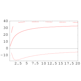
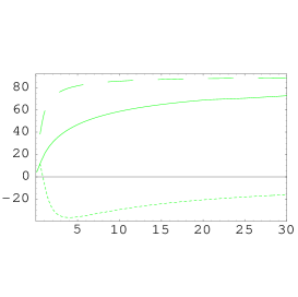
$F_{T}(Q^{2})$
$x_{B}=10^{-2}$	$x_{B}=5\cdot 10^{-3}$	$x_{B}=10^{-3}$
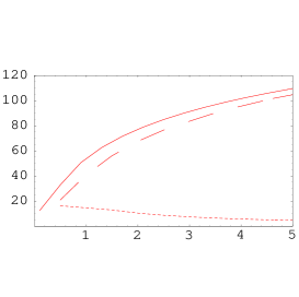
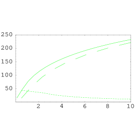
$F_{L}^{D}(Q^{2})$
$x_{B}=10^{-2}$	$x_{B}=5\cdot 10^{-3}$	$x_{B}=10^{-3}$
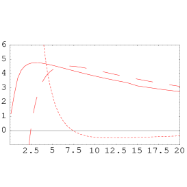
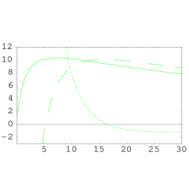
$F_{T}^{D}(Q^{2})$
$x_{B}=10^{-2}$	$x_{B}=5\cdot 10^{-3}$	$x_{B}=10^{-3}$

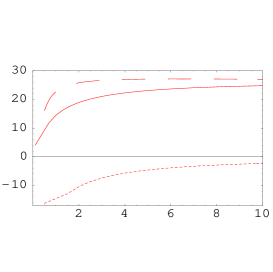
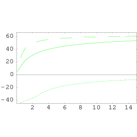
Figure 4: Different twists contributions to the various structure functions for DIS on nucleus $A$=238 ($U$): leading twist (at high $Q^{2}$) – dashed line, next-to-leading – dotted one, exact structure function – solid curve.

To estimate the contributions of the different twists to various structure functions we perform calculations using Eq. (20),Eq. (22) and Eq. (23). Note, that Eq. (20) and Eq. (22) are valid only in the massless limit $m_{f}^{2}=0$. As was explained above, this is a good assumption as long as we are not concerned with small $Q^{2}$ behaviour. All our calculations are made for the eRHIC kinematical region. The results of the calculations for Zn ($A$=30), Sn ($A$=119) and U ($A$=238) are shown in Figs. 2,3 and 4. The following important effects are clearly seen when we compare the contributions of first two non-vanishing twists:

1. In all structure functions except $F_{L}$ there is a scale $\hat{Q}^{2}$ specific for the particular structure function where these two twists are equal. $\hat{Q}^{2}$ is largest for $F_{L}^{D}$;

2. $\hat{Q}^{2}$ grows as $x_{B}$ decreases and $A$ increases;

3. twist-4 in $F_{L}$ cancels numerically with twist-4 in $F_{2}$ in the region of $Q^{2}$ where twist-4 is significant (low $Q^{2}$). This is a reason for measuring the polarized structure functions instead of the total one.

In Figs. 5 and 6 we plotted the ratios $F_{L}/F_{T}\,(x_{B},Q^{2},A)$ and $F_{L}^{D}/F_{T}^{D}\,(x_{B},Q^{2},A)$ correspondingly versus $Q^{2}$. The calculations were performed with formulae Eq. (11) and Eq. (12) not neglecting the mass of the quark $m_{f}$. As is expected on theoretical grounds[7] the ratio has a maximum which increases as $x_{B}$ decreases and $A$ increases. It occurs at $Q^{2}_{max}\gg m_{f}^{2}$ which implies that we are sufficiently distant from the confinement region. However, it differs numerically for inclusive and diffractive ratios. This in turn implies that the SC will be still small at eRHIC.

In Figs. 7 and 8 we show the behavior of $Q^{2}_{max}(x_{B},A)$ as a function of $x_{B}$ and $A$. Note in Fig. 8 that $Q^{2}_{max}\sim A^{0.25}$. If the SC were absent we would expect that $Q^{2}_{max}$ not to depend on $A$, while in saturation regime $Q^{2}_{max}\sim A^{2/3}$. This confirms once more our conclusion that the kinematical region of eRHIC is intermediate between the linear and the saturation regimes.

4 Conclusions

The goal of our work is to understand to what extent the high parton density regime of QCD could manifest itself in DIS experiments at eRHIC where the density of partons could be large enough to make shadowing corrections significant despite the fact that energies are much smaller than that achieved at HERA for DIS on nucleons.

The eikonal approach, developed in Refs. [12, 19, 15] was used for the first estimates of the manifestation of the saturation scale in deep inelastic scattering with nuclei. It has been argued that it provides a reasonable first iteration to the exact evolution equation. We realize that it is not clear whether the equations written in the leading $\ln(1/x_{B})$ approximation are valid in the kinematical region of our interest. However, we believe that our calculations give a reasonable estimate for the magnitude of the effect and of the kinematic region where this effect could be observed experimentally.

We observed two manifestations of the saturation scale:

1. The position of maxima in ratios $F_{L}/F_{T}$ and $F_{L}^{D}/F_{T}^{D}$ ($Q^{2}_{max}$) is intimely related to the saturation scale $Q_{s}^{2}(x_{B})$. $Q^{2}_{max}$ shows $x_{B}$ and $A$ dependence typical for the saturation scale (see Figs. 7 and 8);

2. The results of our calculations show that there exists a scale at which the twist expansion breaks down since all twists become of the same order. We can use the DGLAP evolution equations only for $Q^{2}$ larger than this scale. The energy ($x_{B}$) and $A$ dependence of this scale gives us hope that the experimental data for deep inelastic scattering with nuclei will help to separate leading and higher twists contributions. In the case of nucleon deep inelastic scattering such a separation appears to be a rather difficult task which has not been performed until now.

With this paper we started a systematic analysis of possible manifestation of gluon saturation phenomena in deep inelastic scattering on nuclei. We hope that our estimates will be useful for planning of future experiments especially at eRHIC.

Acknowledgments

We thank Jochen Bartels, Krzysztof Golec-Biernat, Dima Kharzeev and Yura Kovchegov for very fruitful discussions of saturation phenomena.

This paper in part was supported by BSF grant # 9800276. The work of L.McL. was supported by the US Department of Energy (Contract # DE-AC02-98CH10886). The research of E.L., K.T. , E.G. and U.M. was supported in part by the Israel Science Foundation, founded by the Israeli Academy of Science and Humanities.

$F_{L}(Q^{2})$
$x_{B}=10^{-2}$	$x_{B}=5\cdot 10^{-3}$	$x_{B}=10^{-3}$
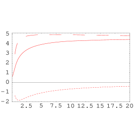
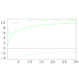
$F_{T}(Q^{2})$
$x_{B}=10^{-2}$	$x_{B}=5\cdot 10^{-3}$	$x_{B}=10^{-3}$
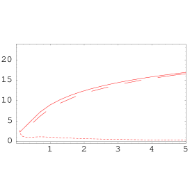
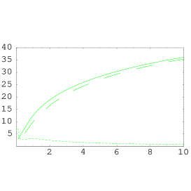
$F_{L}^{D}(Q^{2})$
$x_{B}=10^{-2}$	$x_{B}=5\cdot 10^{-3}$	$x_{B}=10^{-3}$
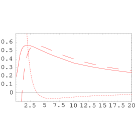
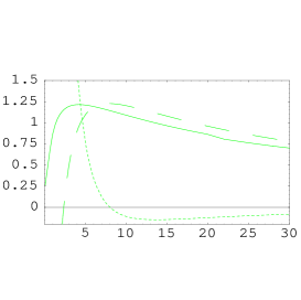
$F_{T}^{D}(Q^{2})$
$x_{B}=10^{-2}$	$x_{B}=5\cdot 10^{-3}$	$x_{B}=10^{-3}$

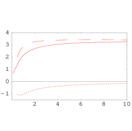
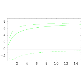
Figure 2: Different twists contributions to the various structure functions for DIS on nucleus $A$=30: leading twist (at high $Q^{2}$) – dashed line, next-to-leading – dotted one, exact structure function – solid curve.

$F_{L}(Q^{2})$
$x_{B}=10^{-2}$	$x_{B}=5\cdot 10^{-3}$	$x_{B}=10^{-3}$
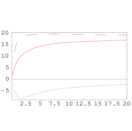
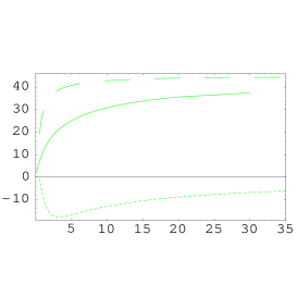
$F_{T}(Q^{2})$
$x_{B}=10^{-2}$	$x_{B}=5\cdot 10^{-3}$	$x_{B}=10^{-3}$
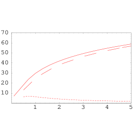
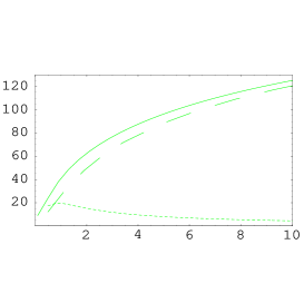
$F_{L}^{D}(Q^{2})$
$x_{B}=10^{-2}$	$x_{B}=5\cdot 10^{-3}$	$x_{B}=10^{-3}$
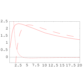
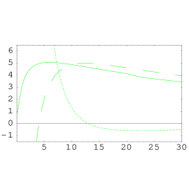
$F_{L}^{D}(Q^{2})$
$x_{B}=10^{-2}$	$x_{B}=5\cdot 10^{-3}$	$x_{B}=10^{-3}$

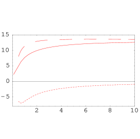
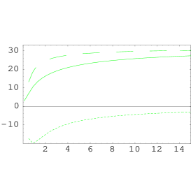
Figure 3: Different twists contributions to the various structure functions for DIS on nucleus $A$=119: leading twist (at high $Q^{2}$) – dashed line, next-to-leading – dotted one, exact structure function – solid curve.

Figure 5: Ratio $F_{L}/F_{T}$ versus $Q^{2}$ for different $x_{B}$ and $A$.

Figure 6: Ratio $F_{L}^{D}/F_{T}^{D}$ versus $Q^{2}$ for different $x_{B}$ and $A$.

Figure 7: Scaling of $Q_{max}^{2}$ with $x_{B}$: maxima of ratios of $F_{L}/F_{T}$ and $F_{L}^{D}/F_{T}^{D}$ versus $\log_{10}(1/x_{B})$ for different $A$.

Figure 8: Scaling of $Q_{max}^{2}$ with $A$: $\ln$ of maxima of ratios of $F_{L}/F_{T}$ and $F_{L}^{D}/F_{T}^{D}$ versus $\ln A$ for different $x_{B}$.

References

- [1] L.V. Gribov, E.M. Levin and M.G. Ryskin, Phys. Rep. 100:1 (1983).
- [2] A.H. Mueller and J. Qiu, Nucl. Phys. B268:427 (1996).
- [3] L. McLerran and R. Venugopalan, Phys. Rev. D49:2233,3352 (1994), Phys. Rev. D50:2225 (1994), Phys. Rev. D53:458 (1996), Phys. Rev. D59:094002 (1999).
- [4] E. Levin and M.G. Ryskin, Phys. Rep. 189:267 (1990); J.C.Collins and J. Kwiecinski, Nucl. Phys. B335:89 (1990); J. Bartels, J. Blumlein and G. Shuler, Z. Phys. C50:91 (1991); E. Laenen and E. Levin, Ann. Rev. Nucl. Part. Sci. 44:199 (1994) and references therein; A.L. Ayala, M.B. Gay Ducati and E.M. Levin, Nucl. Phys. B493:305 (1997), Nucl. Phys. B510:355 (1998); Yu. Kovchegov, Phys. Rev. D54:5463 (1996); Phys. Rev. D55:5445 (1997), Phys. Rev. D60:034008 (1999); A.H. Mueller, Nucl. Phys. B572:227 (2000), Nucl. Phys. B558:285 (1999); Yu. V. Kovchegov, A.H. Mueller, Nucl. Phys. B529:451 (1998); M. Braun LU-TP-00-06,hep-ph/0001268.
- [5] Yu. V. Kovchegov, Phys. Rev. D60:034008 (1999).
- [6] I. Balitsky Nucl. Phys. B463:1996 (99).
- [7] Yu. V. Kovchegov, Phys. Rev. D61:074018 (2000); E. Levin and K. Tuchin, Nucl. Phys. B573:833 (2000).
- [8] J. Jalilian-Marian, A. Kovner, L. McLerran and H. Weigert, Phys. Rev. DD55:5414 (1997); J. Jalilian-Marian, A. Kovner and H. Weigert, Phys. Rev. D59:014015 (1999); J. Jalilian-Marian, A. Kovner and H. Weigert, Phys. Rev. D59:014015 (1999); J. Jalilian-Marian, A. Kovner, A. Leonidov and H. Weigert, Phys. Rev. D59:014014,034007 (1999); Erratum-ibid. Phys. Rev. D59:099903 (1999); A. Kovner, J.Guilherme Milhano and H. Weigert, OUTP-00-10P, NORDITA-2000-14-HE, hep-ph/0004014; H. Weigert, NORDITA-2000-34-HE, hep-ph/0004044.
- [9] J. Bartels, K. Golec-Biernat and K. Peters, hep-ph/0003042.
- [10] K. Golec-Biernat and M. Wusthoff, Phys. Rev. D59:1999 (014017), Phys. Rev. D60:1999 (114023).
- [11] ZEUS collaboration: J. Breitweg et al., Eur. Phys. J.C6:43 (1999); H. Abramowicz and J.B. Dainton, J. Phys. G22:911 (1996).
- [12] A. Zamolodchikov, B. Kopeliovich and L. Lapidus, JETP Lett. 33:612 (1981); E.M. Levin and M.G. Ryskin, Sov. J. Nucl. Phys. 45:150 (1987); A.H. Mueller, Nucl. Phys. B335:115 (1990).
- [13] A.H. Mueller, Nucl. Phys. B415:373 (1994).
- [14] N.N. Nikolaev and B.G. Zakharov, Z. Phys. C49:607 (1991), plb2604141991; E.M. Levin, A.D. Martin, M.G. Ryskin and T. Teubner, Z. Phys. C74:671 (1997).
- [15] H. Abramowicz, L. Frankfurt and M. Strikman,Surveys High Energ.Phys. bf 11:51 (1997) and references therein; B.Blaettel,G. Baym, L. L. Frankfurt, H. Heiselberg and M. Strikman, Phys. Rev. D47:2761 (1993); A.L. Ayala, M.B. Gay Ducati and E.M. Levin, Nucl. Phys. B493:305 (1997), Nucl. Phys. B510:355 (1998) and references therein; E. Gotsman, E. Levin and U. Maor, Phys. Lett. B403:120 (1997), Nucl. Phys. B493:354 (1997), Nucl. Phys. B464:251 (1996); Yu. V. Kovchegov and L. McLerran, Phys. Rev. D60:054025 (1999).
- [16] E. Gotsman, E. Levin, M. Lublinsky, U. Maor and K. Tuchin, TAUP-2639-2000,hep-ph/0007261.
- [17] E. Gotsman, E. Levin, M. Lublinsky, U. Maor and K. Tuchin, TAUP-2605-1999 hep-ph/9911270.
- [18] Yu. V. Kovchegov and L. McLerran, Phys. Rev. D60:054025 (1999).
- [19] A.L. Ayala, M.B. Gay Ducati, E.M. Levin, Nucl. Phys. B493:1997 (305).
-
[20]
J. Bartels, Z. Phys. C60:1993 (471); Phys. Lett. B298:1993 (204);
E. Levin, M. Ryskin and A. Shuvaev, Nucl. Phys. B387:1992 (589). - [21] A.L. Ayala, M.B. Gay Ducati, E.M. Levin, Nucl. Phys. B511:1998 (355).
- [22] H. Bateman and A. Erdelyi, Higher transcendental functions, v.1, McGraw-Hill, 1953.
- [23] M. Glück, E. Reya and A. Vogt, Z. Phys. C67:433 (1995).
- [24] M. Glück, E. Reya and A. Vogt, Z. Phys. C5:461 (1998).