We construct and discuss a ”realistic” example of SUSY $SU(5)$ GUT model, with an additional $U(1)$ flavour symmetry, that is not plagued by the need of large fine tunings, like those associated with doublet-triplet splitting in the minimal model, and that leads to an acceptable phenomenology. This includes coupling unification with a value of $\alpha_{s}(m_{Z})$ in much better agreement with the data than in the minimal version, an acceptable hierarchical pattern for fermion masses and mixing angles, also including neutrino masses and mixings, and a proton decay rate compatible with present limits (but the discovery of proton decay should be within reach of the next generation of experiments). In the neutrino sector the preferred solution is one with nearly maximal mixing both for atmospheric and solar neutrinos.

1 Introduction

The idea that all particle interactions merge into a unified theory [1] at very high energies is so attractive that this concept has become widely accepted by now. The quantitative success of coupling unification in Supersymmetric (SUSY) Grand Unified Theories (GUT’s) has added much support to this idea [2]. The recent developments on neutrino oscillations [3], pointing to lepton number violation at large scales, have further strengthened the general confidence. However the actual realization of this idea is not precisely defined. On the one hand, at the Planck scale, $M_{Pl}$, the unification of gravity with gauge interactions is a general property of superstring theories. On the other hand, in simple GUT models gauge interactions are unified at a distinctly lower mass scale $M_{GUT}$ within the context of a renormalizable gauge theory. But this neat separation between gauge unification and merging with gravity is not at all granted. The gap between $M_{GUT}$ and $M_{Pl}$ could be filled up by a number of threshold effects and several layers of additional states. Also, coupling unification could be realized without gauge unification, as suggested in some versions of superstring theory or in flipped $SU(5)$.

Assuming gauge unification, minimal models of GUT’s based on $SU(5)$, $SO(10)$, … have been considered in detail. Also, many articles have addressed particular aspects of GUT’s models like proton decay, fermion masses and, recently, neutrino masses and mixings. But minimal models are not plausible as they need a large amount of fine tuning and are therefore highly unnatural (for example with respect to the doublet-triplet splitting problem or proton decay). Also, analyses of particular aspects of GUT’s often leave aside the problem of embedding the sector under discussion into a consistent whole. So the problem arises of going beyond minimal toy models by formulating sufficiently realistic, not unnecessarily complicated, relatively complete models that can serve as benchmarks to be compared with experiment. More appropriately, instead of ”realistic” we should say ”not grossly unrealistic” because it is clear that many important details cannot be sufficiently controlled and assumptions must be made. The model we aim at should not rely on large fine tunings and must lead to an acceptable phenomenology. This includes coupling unification with an acceptable value of $\alpha_{s}(m_{Z})$, given $\alpha$ and $sin^{2}\theta_{W}$ at $m_{Z}$, compatibility with the more and more stringent bounds on proton decay [4, 5], agreement with the observed fermion mass spectrum, also considering neutrino masses and mixings and so on. The success or failure of the program of constructing realistic models can decide whether or not a stage of gauge unification is a likely possibility.

Prompted by recent neutrino oscillation data some new studies on realistic GUT models have appeared in the context of $SO(10)$ or larger groups [6]. In the present paper we address the question whether the smallest SUSY $SU(5)$ symmetry group can still be considered as a basis for a realistic GUT model. We indeed present an explicit example of a realistic $SU(5)$ model, which uses a $U(1)$ flavour symmetry as a crucial ingredient. In principle the flavour symmetry could be either global or local. We tentatively assume here that the flavour symmetry is global. This is more in the spirit of GUT’s in the sense that all gauge symmetries are unified. The associated Goldstone boson receives a mass from the anomaly. Such a pseudo-Goldstone boson can be phenomenologically acceptable in view of the existing limits on axion-like particles [7].

In this model the doublet-triplet splitting problem is solved by the missing partner mechanism [8] stabilized by the flavour symmetry against the occurrence of doublet mass lifting due to non renormalizable operators. Relatively large representations (50, $\overline{50}$, 75) have to be introduced for this purpose. A good effect of this proliferation of states is that the value of $\alpha_{s}(m_{Z})$ obtained from coupling unification in the next to the leading order perturbative approximation receives important negative corrections from threshold effects near the GUT scale. As a result, the central value changes from $\alpha_{s}(m_{Z})\approx 0.130$ in minimal SUSY $SU(5)$ down to $\alpha_{s}(m_{Z})\approx 0.116$, in better agreement with observation [9, 10, 11]. The same $U(1)$ flavour symmetry that stabilizes the missing partner mechanism is used to explain the hierarchical structure of fermion masses. In the neutrino sector, the mass matrices already proposed in a previous paper by two of us are reproduced [12]. The large atmospheric neutrino mixing is due to a large left-handed mixing in the lepton sector that corresponds to a large right-handed mixing in the down quark sector. In the present particular version maximal mixing also for solar neutrinos is preferred. A possibly problematic feature of the model is that, beyond the unification point, when all the states participate in the running, the asymptotic freedom of $SU(5)$ is destroyed by the large number of matter fields. As a consequence, the coupling increases very fast and the theory becomes non perturbative below $M_{Pl}$. In the past models similar to ours have been considered, but were discarded just because they contain many additional states and tend to become non perturbative between $M_{GUT}$ and $M_{Pl}$. We instead argue that these features are not necessarily bad. While the predictivity of the theory is reduced because of non renormalizable operators that are only suppressed by powers of $M_{GUT}/\Lambda$ with $\Lambda<M_{Pl}$, still these corrections could explain the distortions of the mass spectrum with respect to the minimal model, the suppression of proton decay and so on. However, it is certainly true that also in this case, as for any other known realistic model, the resulting construction is considerably more complicated than in the corresponding minimal model.

2 The Model

The symmetry of the model is SUSY $SU(5)\otimes U(1)$. We call $Q$ the charge associated with $U(1)$. The superpotential of the model has three parts:

$$w=w_{1}+w_{2}+w_{3}~{}~{}~{}~{}.$$ (1)

The $w_{1}$ term only contains the field $Y$ of the representation 75 of $SU(5)$ with $Q=0$:

$$w_{1}=c_{1}~{}Y^{3}+M_{Y}~{}Y^{2}~{}~{}~{}~{}~{}.$$ (2)

The effect of $w_{1}$ is to provide $Y$ with a vev of order $M_{Y}/c_{1}\approx M_{Y}\approx M_{GUT}$ and to give a mass to all physical components of $Y$, i.e. those that are not absorbed by the Higgs mechanism (the 75 uniquely breaks $SU(5)$ down to $SU(3)\otimes SU(2)\otimes U(1)$).

The $w_{2}$ term induces the doublet-triplet splitting:

$$w_{2}=c_{2}~{}HYH_{50}~{}+~{}c_{3}\bar{H}YH_{\overline{50}}~{}+~{}c_{4}~{}H_{50}{H_{\overline{50}}}X~{}~{}~{}.$$ (3)

Here $H$ and $\bar{H}$ are the usual pentaplets of Higgs fields, except that now they carry non opposite $Q$ charges. It is not restrictive to take $c_{2}$, $c_{3}$ and $c_{4}$ real and positive. The renormalizable couplings that appear in $w_{2}$ are the most general allowed by the $SU(5)$ and $Q$ assignments of the fields in eq. (3) which are given as follows:

$${\rm field}~{}~{}~{}~{}~{}~{}~{}~{}~{}Y~{}~{}~{}~{}~{}~{}~{}~{}~{}H~{}~{}~{}~{}~{}~{}~{}~{}~{}\bar{H}~{}~{}~{}~{}~{}~{}~{}~{}~{}H_{50}~{}~{}~{}~{}~{}~{}~{}~{}~{}{H_{\overline{50}}}~{}~{}~{}~{}~{}~{}~{}~{}~{}X$$

$$SU(5)~{}~{}~{}~{}~{}~{}~{}~{}~{}75~{}~{}~{}~{}~{}~{}~{}~{}~{}5~{}~{}~{}~{}~{}~{}~{}~{}~{}~{}\bar{5}~{}~{}~{}~{}~{}~{}~{}~{}~{}~{}50~{}~{}~{}~{}~{}~{}~{}~{}~{}~{}~{}\bar{50}~{}~{}~{}~{}~{}~{}~{}~{}~{}~{}~{}1$$

$$~{}~{}~{}~{}Q~{}~{}~{}~{}~{}~{}~{}~{}~{}0~{}~{}~{}~{}~{}~{}~{}~{}-q~{}~{}~{}~{}~{}~{}~{}~{}~{}q-1~{}~{}~{}~{}~{}q~{}~{}~{}~{}~{}~{}~{}~{}~{}~{}1-q~{}~{}~{}~{}~{}~{}-1$$ (4)

The value of $q$ will be specified later. At the minimum of the potential, in the limit of unbroken SUSY, the vevs of the fields $H$, $\bar{H}$, $H_{50}$ and ${H_{\overline{50}}}$ all vanish, while the $X$ vev remains undetermined. As we shall see, when SUSY is softly broken the light doublets in $H$ and $\bar{H}$ acquire a small vev while the $X$ vev will be fixed near the cut-off $\Lambda$, of the order of the scale between $M_{GUT}$ and $M_{Pl}$ where the theory becomes strongly interacting (we shall see that we estimate this scale at around $10-20~{}M_{GUT}$, large enough that the approximation of neglecting terms of order $M_{GUT}/\Lambda$ is not unreasonable). The missing partner mechanism to solve the doublet-triplet splitting problem occurs because the 50 contains a $(\bar{3},1)$, i.e. a coloured antitriplet, $SU(2)$ singlet (of electric charge 1/3) but no colourless doublet (1,2). The $U(1)$ flavour symmetry protects the doublet Higgs to take mass from radiative corrections because no $H\bar{H}$ mass term is allowed. Also no non renormalizable terms of the form $H\bar{H}Y^{m}X^{n}$ $(m,n\geq 0)$ are possible, because $X$ has a negative $Q$ charge. This version of the missing partner mechanism was introduced in ref. [13] and overcomes the observation in ref. [14] that, in general, non renormalizable interactions spoil the mechanism. The Higgs colour triplets mix with the analogous states in the 50 and the resulting mass matrix is of the see-saw form:

$$\hat{m}_{T}=\left[\matrix{0&c_{2}\langle Y\rangle\cr c_{3}\langle Y\rangle&c_{4}\langle X\rangle}\right]~{}~{}~{}~{}~{}.$$ (5)

Defining $m_{\phi}=c_{4}\langle X\rangle$ the eigenvalues of the matrix $\hat{m}_{T}\hat{m}_{T}^{\dagger}$ are the squares of:

$$m_{T1,2}=\frac{1}{2}\left[\sqrt{m_{\phi}^{2}+(c_{2}+c_{3})^{2}\langle Y\rangle^{2}}\pm\sqrt{m_{\phi}^{2}+(c_{2}-c_{3})^{2}\langle Y\rangle^{2}}\right]~{}~{}~{}.$$ (6)

Note that $m_{T1}m_{T2}=c_{2}c_{3}\langle Y\rangle^{2}$. The effective mass that enters in the dimension 5 operators with $|\Delta B=1|$ is

$$m_{T}=\frac{{{m_{T}}_{1}}{{m_{T}}_{2}}}{m_{\phi}}=\frac{c_{2}c_{3}}{c_{4}}\frac{\langle Y\rangle^{2}}{\langle X\rangle}~{}~{}~{}.$$ (7)

The $w_{3}$ term contains the Yukawa interactions of the quark and lepton fields $\Psi_{10}$, $\Psi_{\bar{5}}$ and $\Psi_{1}$, transforming as the representations 10, $\bar{5}$ and 1 of SU(5) respectively. We assume an exact $R$-parity discrete symmetry under which $\Psi_{10}$, $\Psi_{\bar{5}}$ and $\Psi_{1}$ are odd whereas $H$, $\bar{H}$, $H_{50}$ and ${H_{\overline{50}}}$ are even. The $w_{3}$ term is symbolically given by

$$w_{3} = \Psi_{10}G_{u}(X,Y)\Psi_{10}H~{}+~{}\Psi_{10}G_{d}(X,Y)\Psi_{\bar{5}}\bar{H}~{}+~{}\Psi_{\bar{5}}G_{\nu}(X,Y)\Psi_{1}H$$ (8)

$$+ M\Psi_{1}G_{M}(X,Y)\Psi_{1}~{}+~{}\Psi_{10}{G_{\overline{50}}}(X,Y)\Psi_{10}H_{{\overline{50}}}~{}~{}~{}.$$

The Yukawa matrices $G_{u}$, $G_{d}$, $G_{\nu}$, $G_{M}$ and ${G_{\overline{50}}}$ depend on $X$ and $Y$ and the associated mass matrices on their vevs. The last term does not contribute to the mass matrices because of the vanishing vev of ${H_{\overline{50}}}$, but is important for proton decay. The pattern of fermion masses is determined by the $U(1)$ flavour symmetry that fixes the powers of $\lambda\equiv\langle X\rangle/\Lambda$ for each entry of the mass matrices. In fact $X$ is the only field with non vanishing $Q$ that takes a vev. The powers of $\lambda$ in the mass terms are fixed by the $Q$ charges of the matter field $\Psi$ and of the Higgs fields $H$ and $\bar{H}$. We can then specify the charge $q$ that appears in (4) and the $Q$ charges of the matter fields $\Psi$ in order to obtain realistic textures for the fermion masses. We choose $q=2$, so that we have from the table in (4):

$$Q(H)=-2~{}~{}{\rm and}~{}~{}Q(\bar{H})=1~{}~{}~{},$$ (9)

and, for matter fields

$$Q(\Psi_{10})=(4,3,1)~{}~{}~{},~{}~{}~{}~{}~{}~{}~{}Q(\Psi_{\bar{5}})=(4,2,2)~{}~{}~{},~{}~{}~{}~{}~{}~{}~{}Q(\Psi_{1})=(1,-1,0)~{}~{}~{}.$$ (10)

The Yukawa mass matrices are of the form:

$$G_{r}(\langle X\rangle,\langle Y\rangle)_{ij}~{}=~{}\lambda^{n_{ij}}G_{r}(\langle Y\rangle)_{ij},~{}~{}~{}~{}~{}~{}~{}~{}{r=u,d,\nu,M}~{}~{}~{}.$$ (11)

We expand $G_{r}(\langle Y\rangle)_{ij}$ in powers of $\langle Y\rangle$ and consider the lowest order term at first. Taking $G_{r}(0)_{ij}$ of order 1 and $n_{ij}$ as dictated by the above charge assignments we obtain :

$$\begin{array}[]{lr}m_{u}~{}=~{}\frac{1}{\sqrt{2}}\left[\matrix{\lambda^{6}&\lambda^{5}&\lambda^{3}\cr\lambda^{5}&\lambda^{4}&\lambda^{2}\cr\lambda^{3}&\lambda^{2}&1}\right]~{}v_{u}~{}~{}~{}~{},&~{}~{}~{}~{}~{}~{}~{}~{}~{}~{}m_{d}~{}=~{}m_{e}^{T}~{}=~{}\frac{1}{\sqrt{2}}\left[\matrix{\lambda^{5}&\lambda^{3}&\lambda^{3}\cr\lambda^{4}&\lambda^{2}&\lambda^{2}\cr\lambda^{2}&1&1}\right]~{}v_{d}\lambda^{4}~{}~{}~{}~{}~{},\\ &\\ m_{\nu}~{}=~{}\frac{1}{\sqrt{2}}\left[\matrix{\lambda^{3}&\lambda&\lambda^{2}\cr\lambda&0&1\cr\lambda&0&1}\right]~{}v_{u}~{}~{}~{}~{},&m_{maj}~{}=~{}\left[\matrix{\lambda^{2}&1&\lambda\cr 1&0&0\cr\lambda&0&1}\right]~{}M~{}~{}~{}~{}.\end{array}$$ (12)

For a correct first approximation of the observed spectrum we need $\lambda\approx\lambda_{C}\approx 0.22$, $\lambda_{C}$ being the Cabibbo angle. These mass matrices closely match those of ref. [12], with two important special features. First, we have here that $\tan\beta=v_{u}/v_{d}\approx m_{t}/m_{b}\lambda^{4}$, which is small. The factor $\lambda^{4}$ is obtained as a consequence of the Higgs and matter fields charges Q, while in ref. [12] the $H$ and $\bar{H}$ charges were taken as zero. We recall that a value of $\tan\beta$ near 1 is an advantage for suppressing proton decay. A small range of $\tan\beta$ around one is currently disfavored by the negative results of the SUSY Higgs search at LEP [15]. Of course we could easily avoid this range, if necessary. Second, the zero entries in the mass matrices of the neutrino sector occur because the negatively $Q$-charged $X$ field has no counterpart with positive $Q$-charge. Neglected small effects could partially fill up the zeroes. As explained in ref. [12] these zeroes lead to near maximal mixing also for solar neutrinos.

A problematic aspect of this zeroth order approximation to the mass matrices is the relation $m_{d}=m_{e}^{T}$. This equality is good as an order of magnitude relation because relates large left-handed mixings for leptons to large right handed mixings for down quarks [12, 16]. However the implied equalities $m_{b}/m_{\tau}=m_{s}/m_{\mu}=m_{d}/m_{e}=1$ are good only for the third generation while need to be corrected by factors of 3 for the first two generations. The necessary corrective terms can arise from the neglected terms in the expansion in $\langle Y\rangle$ of $G_{r}(\langle Y\rangle)_{ij}$ [17]. The higher order terms correspond to non renormalizable operators with the insertion of $n$ factors of the 75, which break the transposition relation between $m_{d}$ and $m_{e}$. For this purpose we would like the expansion parameter $\langle Y\rangle/\Lambda$ to be not too small in order to naturally provide the required factors of 3. We will present in the following explicit examples of parameter choices that lead to a realistic spectrum without unacceptable fine tuning.

The breaking of SUSY fixes a large vev for the field $X$ by removing the corresponding flat direction, gives masses to s-partners, provides a small mass to the Higgs doublet and introduces a $\mu$ term. Up to coefficients of order one we can write down the terms that break SUSY softly:

$$-{\cal L}_{soft}~{}=~{}m^{2}|x|^{2}+m^{2}|c|^{2}~{}+~{}m^{2}|\bar{c}|^{2}~{}+m(c\bar{c}x~{}+~{}h.c.)~{}+.....$$ (13)

where $c$, $\bar{c}$ and $x$ denote the scalar components of $H_{50}$, ${H_{\overline{50}}}$ and $X$ respectively, and dots stand for the remaining soft breaking terms, including mass terms for the scalar components of the Higgs doublet fields . In the SUSY limit and neglecting the mixing between the $(50,{\overline{50}})$ and the $(5,\bar{5})$ sectors, fermions and scalars in the $50$ and ${\overline{50}}$ have a common squared mass $c^{2}_{4}x^{2}$. When SUSY is broken by the soft terms for each fermion of mass $c_{4}x$ there are two bosons of squared masses $c^{2}_{4}x^{2}+m^{2}\pm mx$. The $x$ terms in the scalar potential at one loop accuracy are given by:

$$V = m^{2}x^{2}+\frac{50}{64\pi^{2}}\left\{2(c^{2}_{4}x^{2}+m^{2}+mx)^{2}\left[\log\left({\frac{c^{2}_{4}x^{2}+m^{2}+mx}{\Lambda^{2}}}\right)-3/2\right]\right.$$ (14)

$$+ 2(c^{2}_{4}x^{2}+m^{2}-mx)^{2}\left[\log\left({\frac{c^{2}_{4}x^{2}+m^{2}-mx}{\Lambda^{2}}}\right)-3/2\right]$$

$$- \left.4c^{4}_{4}x^{4}\left[\log\left({\frac{c^{2}_{4}x^{2}}{\Lambda^{2}}}\right)-3/2\right]\right\}$$

A numerical study of this potential in the limit $m\ll\Lambda$ and for $c_{4}$ of order one, shows that the minimum is at $x$ of order $\Lambda$ (somewhat smaller than $\Lambda$ but close to it). The expression for $V$ in eq. (14) provides a good approximation of the scalar potential only in a small region around $\Lambda$. Outside this region the perturbative approximation will break down. We take our numerical analysis as an indication that the minimum occurs near $\Lambda$ and we assume that the true minimum occurs at $x=\langle X\rangle=0.25\Lambda$, that is $\lambda=0.25$. The complex field $x$ describes two physical scalar particles. The one associated to the real part of $x$ has a mass of order $m$ and couplings to the ordinary fermions suppressed by $1/\Lambda$. The particle associated to the imaginary part of $x$ is massless only in the tree approximation. Due to the anomaly of the related $U(1)_{Q}$ current the particle acquires a mass of order $f_{\pi}m_{\pi}/\langle X\rangle$. Cosmological bounds on $\langle X\rangle$ have been recently reconsidered in ref. [7] where it has been observed that $\langle X\rangle$ of the order of the grand unification scale is not in conflict with observational data.

An alternative possibility is to assume that the $U(1)$ symmetry is local [13]. In this case the supersymmetric action contains a Fayet-Iliopoulos term and the associated D-term in the scalar potential provides a large vev for $x$, of the order of the cut-off scale $\Lambda$.

A $\mu$ term for the fields $H$ and $\bar{H}$ of the appropriate order of magnitude can be generated according to the Giudice-Masiero mechanism [18]. Assume that the breaking of SUSY is induced by the $\theta^{2}$ component of a chiral (effective) superfield $S$, singlet under $SU(5)$ with $Q=0$. In the Kahler potential a term of the form

$$K~{}=~{}\frac{S^{\dagger}X^{\dagger}H\bar{H}}{\Lambda^{2}}+{\rm h.c.}$$ (15)

is allowed. The vevs of $S$ and $X$, $\langle S\rangle\sim\theta^{2}mM_{Pl}$, $\langle X\rangle=\lambda\Lambda$ lead to an equivalent term in the superpotential of the desired form $\mu H\bar{H}$ with $\mu\sim\lambda mM_{Pl}/\Lambda$ which can be considered of the right order.

3 Coupling Unification

It is well known that in the minimal version of SUSY SU(5) the central value of $\alpha_{s}(m_{Z})$ required by the constraint of coupling unification is somewhat large: $\alpha_{s}(m_{Z})\approx 0.13$ [9, 10, 11, 19, 20]. In the model discussed here, where the doublet triplet splitting problem is solved by introducing the $SU(5)$ representations $50$, ${\overline{50}}$ and $75$, the central value of $\alpha_{s}(m_{Z})$ is modified by threshold corrections near $M_{GUT}$ which bring the central value down by a substantial amount so that the final result can be in much better agreement with the observed value. As discussed in refs. [9, 10], this remarkable result arises because the $24$ of the minimal model is replaced by the $75$. The mass splittings inside these representations are dictated by the group embedding of the singlet under $SU(3)\otimes SU(2)\otimes U(1)$ that breaks SU(5). The difference in the threshold contributions from the $24$ and the $75$ has the right sign and amount to bring $\alpha_{s}(m_{Z})$ down even below the observed value. The right value can then be obtained by moving $m_{SUSY}$ and $m_{T}$ in a reasonable range. The difference in the favored value of $m_{T}$ with respect to the minimal model in order to reproduce the observed value of $\alpha_{s}(m_{Z})$ goes in the right direction to also considerably alleviate the potential problems from the bounds on proton decay. Note that there are no additional threshold corrections from the $50$ and ${\overline{50}}$ representations because the mass of these states arise from the coupling to the field $X$ which is an $SU(5)$ singlet. Thus there are no mass splittings inside the $50$ and the ${\overline{50}}$ and no threshold contributions. While there is no effect on the value of $\alpha_{s}(m_{Z})$ the presence of the states in the $50$ and ${\overline{50}}$ representations affects the value of the unified coupling at $M_{GUT}$ and also spoils the asymptotic freedom of SU(5) beyond $M_{GUT}$. We find it suggestive that the solution of the doublet triplet splitting problem in terms of the $50$, ${\overline{50}}$ and $75$ representations automatically leads to improve the prediction of $\alpha_{s}(m_{Z})$ and at the same time relaxes the constraints from proton decay. We now discuss this issue in more detail.

Defining in the ${\overline{MS}}$ scheme $\alpha\equiv\alpha_{QED}(m_{Z})$, $\sin^{2}{\theta}\equiv\sin^{2}{\theta}(m_{Z})$, $a_{3}\equiv\alpha_{s}(m_{Z})$, $a_{5}\equiv\alpha_{5}(M_{GUT})$, from the one-loop renormalization group evolution of the couplings in the MSSM with only two light Higgs doublets we have:

$$a_{3}^{(0)}=\frac{28\alpha}{60\sin^{2}{\theta}-12}$$

$$a_{5}^{(0)}=\frac{28\alpha}{36\sin^{2}{\theta}-3}$$

$$\log{(M^{(0)}_{GUT}/m_{Z})}=\frac{\pi(3-8\sin^{2}{\theta})}{14\alpha}$$ (16)

where by $a^{(0)}$ we mean the quantity $a$ in the leading log approximation (LO). The LO results are the same as in minimal SUSY $SU(5)$. For $\alpha^{-1}=127.934$ and $\sin^{2}{\theta}=0.231$ one obtains $a_{3}^{(0)}=0.118$ and $M^{(0)}_{GUT}=2.1~{}10^{16}$ GeV.

To go beyond the LO one must include two-loop effects in the running of gauge couplings, threshold effects at the scale $m_{SUSY}$, close to the electroweak scale, and threshold effects at the large scale $M_{GUT}$. The unification scale $M_{GUT}$ is not univocally defined beyond LO and here we choose to identify it with the mass of the $SU(5)$ superheavy gauge bosons. The results derived in ref. [9] can be written in the following form:

$$a_{3} = \frac{a_{3}^{(0)}}{(1+a_{3}^{(0)}\delta)}$$

$$\delta = k+\frac{1}{2\pi}\log\frac{m_{SUSY}}{m_{Z}}-\frac{3}{5\pi}\log\frac{m_{T}}{M_{GUT}^{(0)}}~{}~{}~{}~{}.$$ (17)

In this expression for $\delta$ the logarithmic term with $m_{SUSY}$ comes from particles with masses near $m_{SUSY}$. Similarly, the logarithmic term with $m_{T}$ arises from particles with masses of order $m_{T}\approx M_{GUT}$. The definition of $m_{T}$ is the mass of Higgs colour triplets in the minimal model or the effective mass, defined in eq. (7), that, in the realistic model, plays the same role for proton decay [9, 10]. The term indicated with $k=k(2)+k(SUSY)+k(M_{GUT})$ contains the contribution of two-loop diagrams to the running couplings, $k(2)$, the threshold contribution of states near $m_{SUSY}$, $k(SUSY)$, and the threshold contribution from states near $M_{GUT}$, $k(M_{GUT})$. The threshold contributions would vanish if all states had the mass $m_{SUSY}$ or $M_{GUT}$ so that only mass splittings contribute to $k(SUSY)$ and $k(M_{GUT})$. The values of $k(2)$ and of $k(SUSY)$ are essentially the same in the minimal and the realistic model: typical values are $k(2)=-0.733$ and $k(SUSY)=-0.510$. The value for $k(SUSY)=-0.510$ corresponds to the representative spectrum displayed in Table 1. The value of $k(M_{GUT})$ is practically zero for the $24$ of the minimal model while we have $k(M_{GUT})=1.857$ for the $75$ of the realistic model. Thus we obtain:

$$k=-0.733-0.510 = -1.243~{}~{}~{}~{}~{}~{}~{}~{}\rm{minimal~{}model}$$

$$k=-0.733-0.510+1.857 = 0.614~{}~{}~{}~{}~{}~{}~{}~{}~{}~{}~{}\rm{realistic~{}model}$$ (18)

This difference is very important and makes the comparison with experiment of the predicted value of $\alpha_{s}(m_{Z})$ much more favorable in the case of the realistic model. In fact for $k$ large and negative as in the minimal model we need to take $m_{SUSY}$ as large as possible and $m_{T}$ as small as possible. But the smaller $m_{T}$ the faster is proton decay. The best compromise is something like $m_{SUSY}\approx 1$ TeV and $m_{T}\approx M_{GUT}^{(0)}$, which leads to $\alpha_{s}(m_{Z})\approx 0.13$ which is still rather large and proton decay is dangerously fast. This is to be confronted with the case of the realistic model where $k$ is instead positive and large enough to drag $\alpha_{s}(m_{Z})$ below the observed value. We now prefer $m_{T}$ to be larger than $M_{GUT}^{(0)}$ by typically a factor of 20-30, which means a factor of 400-1000 of suppression for the proton decay rate with respect to the minimal model. For example, for $m_{SUSY}\approx 0.25$ TeV and $m_{T}\approx 6\cdot 10^{17}$ GeV we obtain $\alpha_{s}(m_{Z})\approx 0.116$ which is acceptable. The predictions for $a_{3}$ versus $(m_{SUSY},m_{T})$ in the minimal and the missing doublet models are shown in fig. 1.

sparticle	mass2
gluinos	$(2.7m_{1/2})^{2}$
winos	$(0.8m_{1/2})^{2}$
higgsinos	$\mu^{2}$
extra Higgses	$m_{H}^{2}$
squarks	$m_{0}^{2}+6m^{2}_{1/2}$
(sleptons)L	$m_{0}^{2}+0.5m^{2}_{1/2}$
(sleptons)R	$m_{0}^{2}+0.15m^{2}_{1/2}$

Table 1. Representative SUSY spectrum. $SU(2)\otimes U(1)$ breaking effects are neglected. The additional freedom related to the parameters $m_{0}$, $m_{1/2}$, $\mu$, $m_{H}$ is here fixed by choosing $0.8m_{0}=0.8m_{1/2}=2\mu=m_{H}$ and taking as a definition $m_{SUSY}\equiv m_{H}$, so that all particle masses can be expressed in term of $m_{SUSY}$. This parametrization leads to $k(SUSY)=-0.510$.

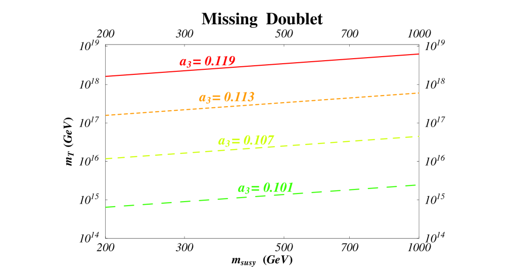
Figure 1: Contours of $a_{3}\equiv\alpha_{s}(m_{Z})$ in the plane $(m_{SUSY},m_{T})$, for the minimal $SU(5)$ and the missing doublet model. The SUSY spectrum is parametrized as in Table 1.

Clearly, there is an uncertainty on $k(SUSY)$, related to the possibility of varying both the parametrization used and the relations assumed between the parameters $m_{0}$, $m_{1/2}$, $\mu$, $m_{H}$. An overall uncertainty of $\pm 0.005$ on $a_{3}$ has been estimated in ref. [19] by scanning many models consistent with electroweak symmetry breaking, a neutral lightest supersymmetric particle and sparticle masses above the experimental bound and below $\sim$ 2 TeV .

Another source of uncertainty on $a_{3}$ is related to the unknown physics above the cut-off scale of the grand unified theory. There can be threshold effects due to new heavy particles or even non perturbative effects that arise in the underlying fundamental theory. These effects can be estimated from the non-renormalizable operators, suppressed by $\langle Y\rangle/\Lambda$, that split the gauge couplings at the scale $M_{GUT}^{(0)}$ [22]. For generic, order one coefficients and barring cancellations among different terms, the presence of these operators may affect $a_{3}$ by additional contributions of about $\pm 0.005M_{Pl}/\Lambda$ [19]. As we will see the model under discussion requires $\Lambda\approx 0.1M_{Pl}$. Therefore, to maintain the good agreement between the experimental and predicted values of $a_{3}$, we need a suppression of this contribution by about a factor of 10, which we do not consider too unnatural.

In view of the large theoretical uncertainties on $a_{3}$ we cannot firmly conclude that the gauge coupling unification fails in the minimal model while it is completely successful in the realistic one. However we find very encouraging that, by solving the doublet-triplet splitting problem within the missing partner model, acceptable values of $a_{3}$ can be easily obtained and that they are directly related to a proton lifetime potentially larger than in the minimal model.

Due to the large matter content the model is not asymptotically free and the gauge coupling constant $\alpha_{5}$ blows up at the scale

$$M_{GUT}~{}~{}{\rm exp}{\displaystyle\left(\frac{\pi}{26a_{5}}\right)}~{}~{}~{}~{}~{}.$$ (19)

Taking into account that threshold effects modify $a_{5}$ with respect the LO value $a_{5}^{(0)}\approx 1/24$, we find that the pole occurs near $10^{17}$ GeV, the precise value depending on the details of the heavy spectrum.

4 Yukawa couplings

To reproduce the fermion mass spectrum we must further specialize the Yukawa couplings introduced in eq. (8):

$$w_{3} = \frac{1}{4}\Psi_{10}^{ab}~{}G_{u}~{}\Psi_{10}^{cd}~{}H^{e}\epsilon_{abcde}+\frac{1}{4}\Psi_{10}^{ab}~{}G_{\overline{50}}~{}\Psi_{10}^{cd}~{}{H_{\overline{50}}}_{abcd}$$ (20)

$$+ \sqrt{2}~{}\Psi_{10}^{ab}~{}G_{d}~{}{\Psi_{\bar{5}}}_{a}~{}{\bar{H}}_{b}+\frac{1}{\Lambda}~{}\sqrt{2}~{}\Psi_{10}^{ab}~{}F_{d}~{}{\Psi_{\bar{5}}}_{c}~{}{\bar{H}}_{d}~{}Y^{cd}_{ab}$$

$$+ \Psi_{1}~{}G_{\nu}~{}{\Psi_{\bar{5}}}_{a}~{}H^{a}-\frac{1}{2}~{}M~{}\Psi_{1}~{}G_{M}~{}\Psi_{1}+...$$

where $G_{r}~{}(r=u,d,\nu,M,{\overline{50}})$ is proportional to $G_{r}(\langle X\rangle,0)$ of eq. (8). We have explicitly introduced a term linear in $Y$, whose couplings are described by the $\langle X\rangle$-dependent matrix $F_{d}$. There are other terms linear in $Y/\Lambda$, not explicitly given above. In particular we may insert $Y/\Lambda$ in the renormalizable term providing masses to the up type quarks. We neglect such a term since, on the one hand, the matrix $G_{u}$ is already sufficient to correctly reproduce the up quark masses and, on the other hand, this operator would not significantly modify the results for proton decay. As we will show, $Y/\Lambda$ is close to 0.1 in our model and higher order terms in the $Y/\Lambda$ expansion can be safely neglected. The interaction term involving ${H_{\overline{50}}}_{abcd}$ does not contribute to the fermion spectrum, but it will be relevant for the proton decay amplitudes.

The term linear in $Y$ in the previous equation is sufficient to differentiate the spectra in the charged lepton and down quark sectors. We get the following Dirac mass matrices:

$$m_{u,\nu}=y_{u,\nu}~{}\frac{v_{u}}{\sqrt{2}}~{}~{}~{},~{}~{}~{}~{}~{}m_{d,e}=y_{d,e}~{}\frac{v_{d}}{\sqrt{2}}~{}~{}~{}~{}~{},$$ (21)

$$\begin{array}[]{lll}y_{u}=G_{u}{}{}{}&&y_{\nu}=G_{\nu}~{}~{}~{}~{}~{},\\ &\\ y_{d}=G_{d}+\displaystyle\frac{\langle Y\rangle}{\Lambda}F_{d}{}{}{}&&y_{e}^{T}=G_{d}-3\displaystyle\frac{\langle Y\rangle}{\Lambda}F_{d}~{}~{}~{},\end{array}$$ (22)

where $v_{u}$, $v_{d}$ and $\langle Y\rangle$ parametrize the vevs of $H$, ${\bar{H}}$ and $Y$ respectively. The fermion spectrum can be easily fitted by appropriately choosing the numerical values of the matrices $G_{u}$, $G_{d}$, $F_{d}$, $G_{\nu}$ and $G_{M}$. The most general fitting procedure would leave a large number of free parameters. Here we limit ourselves to the discussion of one particular example. In agreement with eq. (12), we take:

$$G_{u}=\left[\matrix{(-0.51+0.61i)\lambda^{6}&(0.42-0.70i)\lambda^{5}&(0.27+0.86i)\lambda^{3}\cr(0.42-0.70i)\lambda^{5}&(-0.39+0.52i)\lambda^{4}&(-0.30-1.14i)\lambda^{2}\cr(0.27+0.86i)\lambda^{3}&(-0.30-1.14i)\lambda^{2}&1.39}\right]~{}~{}~{},$$ (23)

$$G_{d}=\lambda^{4}\left[\matrix{(2.39-1.11i)\lambda^{5}&(0.33-0.59i)\lambda^{3}&(0.13+0.45i)\lambda^{3}\cr(0.87+0.55i)\lambda^{4}&(2.76+0.89i)\lambda^{2}&(0.69-0.51i)\lambda^{2}\cr(-1.50+0.94i)\lambda^{2}&(0.45+1.78i)&1.94}\right]~{}~{}~{},$$ (24)

$$\frac{\langle Y\rangle}{\Lambda}F_{d}=\lambda^{4}\left[\matrix{(0.38-0.18i)\lambda^{5}&(-0.16-0.06i)\lambda^{3}&(0.07+0.04i)\lambda^{3}\cr(-0.08-0.05i)\lambda^{4}&(-0.20-0.15i)\lambda^{2}&(0.15-0.11i)\lambda^{2}\cr(-0.09+0.12i)\lambda^{2}&(0.07+0.14i)&-0.19}\right]~{}~{}~{},$$ (25)

$$G_{\nu}=\left[\matrix{(-0.78-0.19i)\lambda^{3}&(0.52-0.34i)\lambda&(1.38+0.39i)\lambda^{2}\cr(-1.23-0.34i)\lambda&0&(1.04+1.31i)\cr(0.45+1.18i)\lambda&0&0.8+1.2i}\right]~{}~{}~{},$$ (26)

$$G_{M}=\left[\matrix{(1.50+0.55i)\lambda^{2}&(1.41+1.19i)&(0.35-1.53i)\lambda\cr(1.41+1.19i)&0&0\cr(0.35-1.53i)\lambda&0&1.26+1.48i}\right]~{}~{}~{}.$$ (27)

While the generic pattern of $G_{u}$, $G_{d}$, $F_{d}$, $G_{\nu}$ and $G_{M}$ is dictated by the $U(1)$ flavour symmetry, the precise values of the coefficients multiplying the powers of $\lambda$ are chosen to reproduce the data. We take $\lambda\equiv\langle X\rangle/\Lambda=0.25$, $\tan\beta=1.5$ and $M=0.9\cdot 10^{15}$ GeV. In SU(5) the matrix $G_{u}$ contains two additional phases [23], $\phi_{1}$ and $\phi_{2}$ that have been set to zero in eq. (23). These phases do not affect the fermion spectrum but enter the proton decay amplitude. When discussing the proton decay we will analyze also the dependence on $\phi_{1}$ and $\phi_{2}$.

From the above matrices we obtain, at the unification scale:

$$\begin{array}[]{lll}m_{t}=200~{}{\rm GeV}&m_{c}=0.27~{}{\rm GeV}&m_{u}=0.9~{}{\rm MeV}\\ m_{b}=1.0~{}{\rm GeV}&m_{s}=26~{}{\rm MeV}&m_{d}=1.1~{}{\rm MeV}\\ m_{\tau}=1.1~{}{\rm GeV}&m_{\mu}=71~{}{\rm MeV}&m_{e}=0.34~{}{\rm MeV}\end{array}$$ (28)

$$|V_{us}|=0.22~{}~{}~{}~{}~{}|V_{ub}|=0.0022~{}~{}~{}~{}~{}|V_{cb}|=0.052~{}~{}~{}~{}~{}J=1.9\cdot 10^{-5}~{}~{}~{},$$ (29)

where $J$ is the CP-violating Jarlskog invariant. In the neutrino sector, we find:

$$m_{1}=0.81\cdot 10^{-3}{\rm eV}~{},~{}~{}~{}~{}m_{2}=0.88\cdot 10^{-3}{\rm eV}~{},~{}~{}~{}~{}m_{3}=0.061~{}{\rm eV}~{}~{}~{}.$$ (30)

More precisely:

$$\Delta m^{2}_{sol}\equiv m_{2}^{2}-m_{1}^{2}=1.1\cdot 10^{-7}~{}{\rm eV}^{2}~{}~{},~{}~{}~{}~{}~{}\Delta m^{2}_{atm}\equiv m_{3}^{2}-m_{2}^{2}=3.7\cdot 10^{-3}~{}{\rm eV}^{2}~{}~{}~{}.$$ (31)

The neutrino mixing angles are

$$\theta_{12}\sim\frac{\pi}{4}~{}~{},~{}~{}~{}~{}~{}\theta_{23}\sim\frac{\pi}{4}~{}~{},~{}~{}~{}~{}~{}\theta_{13}=0.06~{}~{}~{}.$$ (32)

Until now we have not specified the value of $\langle Y\rangle/\Lambda$. We know that $\langle Y\rangle$ should be around $M_{GUT}^{(0)}$. The cut-off $\Lambda$ cannot be too close to $\langle Y\rangle$, otherwise most of the spectrum of the model would lie beyond the cut-off. At the same time $\Lambda$ cannot be too large: it is bounded from above by the scale at which the $SU(5)$ gauge coupling blows up, which, as we see from eq. (19), occurs more or less one order of magnitude below the Planck mass. This is welcome. If, for instance, we take $\langle Y\rangle/\Lambda=0.05-0.1$, it is reasonable to neglect multiple insertions of $Y$ in the Yukawa operators. At the same time, in the example given in eq. (25), the coefficients of the powers of $\lambda$ in $F_{d}$ remain of order one, even if $\langle Y\rangle/\Lambda$ is as small as 0.05. A too large cut-off would have been ineffective in separating down quarks from charged leptons unless we had chosen unnaturally large coefficients in the allowed operators. What is usually considered a bad feature of the missing partner mechanism - the lack of perturbativity before the Planck mass - turns out here to be an advantage to provide a correct description of the fermion spectrum.

The neutrino sector is quite similar to one of the two options described in ref. [12]. We obtain a bimaximal neutrino mixing with the so-called LOW solution to the solar neutrino problem . Within the same $U(1)$ flavour symmetry considered here we could as well reproduce the vacuum oscillation solution, by appropriately tuning the order one coefficients in $G_{\nu}$ and $G_{M}$. We recall that the value of $M$ required to fit the observed atmospheric oscillations is probably somewhat small in the context of $SU(5)$, where a larger scale, closer to the cut-off $\Lambda$, is expected. This feature might be improved by embedding the model in $SO(10)$ where $M$ is directly related to the $B-L$ breaking scale.

In conclusion, the known fermion spectrum can be reproduced starting from a superpotential with order one dimensionless coefficients. Mass matrix elements for charged leptons and down quarks match only within $10-20\%$, due to $\langle Y\rangle/\Lambda\approx 0.1$, and this produces the required difference between the two sectors. The neutrino mixing is necessarily bimaximal in our model, with either the LOW or the vacuum oscillation solution to the solar neutrino problem.

5 Proton Decay

Similarly to the case of minimal $SU(5)$, we expect that the main contribution to proton decay comes from the dimension five operators [24] originating at the grand unified scale when the colour triplet superfields are integrated out [25, 26, 27]. We denote the colour triplets contained in $H$, ${\bar{H}}$, $H_{50}$, ${H_{\overline{50}}}$ by $H_{3u}$, $H_{3d}$, $H^{\prime}_{3d}$ and $H^{\prime}_{3u}$, respectively. The part of the superpotential depending on these superfields reads:

$$w = H_{3u}\left[-\frac{1}{2}QG_{u}Q+U^{c}G_{u}E^{c}\right]$$ (33)

$$+ H_{3d}\left[Q\hat{C}L+U^{c}\hat{D}D^{c}\right]$$

$$+ H^{\prime}_{3u}\left[-\frac{1}{2}QG_{\overline{50}}Q+U^{c}G_{\overline{50}}E^{c}\right]$$

$$+ c_{2}\langle Y\rangle~{}H^{\prime}_{3d}H_{3u}+c_{3}\langle Y\rangle~{}H_{3d}H^{\prime}_{3u}+c_{4}\langle X\rangle~{}H^{\prime}_{3d}H^{\prime}_{3u}+...$$

where

$$\hat{C}=-G_{d}-\frac{\langle Y\rangle}{\Lambda}F_{d}~{}~{},~{}~{}~{}~{}~{}~{}~{}~{}\hat{D}=G_{d}-\frac{\langle Y\rangle}{\Lambda}F_{d}$$ (34)

and $Q$, $L$, $U^{c}$, $D^{c}$ and $E^{c}$ denote as usual the chiral multiplets associated to the three fermion generations. Notice that, at variance with the minimal $SU(5)$ model, an additional interaction term depending on $H^{\prime}_{3u}$ is present. By integrating out the colour triplets we obtain the following effective superpotential:

$$w_{eff}=\frac{1}{m_{T}}\left[Q\hat{A}Q~{}Q\hat{C}L+U^{c}\hat{B}E^{c}~{}U^{c}\hat{D}D^{c}\right]+...$$ (35)

where $m_{T}$ has been defined in eq. (7),

$$\hat{B}=-2\hat{A}=\left(G_{u}-\frac{c_{2}}{c_{4}}\frac{\langle Y\rangle}{\langle X\rangle}G_{\overline{50}}\right)$$ (36)

and dots stand for terms that do not violate baryon or lepton number. Minimal $SU(5)$ is recovered by setting $G_{\overline{50}}=F_{d}=0$. In that case the matrices $\hat{A}$, $\hat{B}$, $\hat{C}$ and $\hat{D}$ are determined by $G_{u}$ (in which now also $\phi_{1}$ and $\phi_{2}$ play a role) and $G_{d}$ and therefore strictly related to the fermionic spectrum [25]. In our case we have a distortion due to the terms proportional to $G_{\overline{50}}$ and $F_{d}$. These distortions have different physical origins. On the one hand the terms containing $F_{d}$ are required to avoid the rigid mass relation of minimal $SU(5)$. They are suppressed by $\langle Y\rangle/\Lambda$ and we expect a mild effect from them [28]. On the other hand the terms containing $G_{\overline{50}}$ are a consequence of the missing doublet mechanism and they might be as important as those of the minimal model.

At lower scales the dimension five operators give rise to the four fermion operators relevant to proton decay, via a “dressing” mainly due to chargino exchange [24, 25, 29]. When considering the operators $QQQL$ the main contribution, here called $L_{1}$, comes from the exchange of a wino . Charged higgsino exchange provides instead the most important dressing of the operators $U^{c}U^{c}D^{c}E^{c}$ [32]. We term $L_{2}$ the leading four-fermion operator in this case. Beyond $L_{1}$ and $L_{2}$ other 6 operators are generated by chargino exchange, 3 from $QQQL$ and 3 from $U^{c}U^{c}D^{c}E^{c}$. The contributions to the proton decay amplitudes from these operators are suppressed by at least $\lambda^{2}$ with respect to those associated to $L_{1}$ and $L_{2}$, and can be safely neglected in the present estimate. $L_{1}$ and $L_{2}$ are given by:

$$L_{1} = C^{1}_{ijkl}~{}(\nu_{l}d_{i})~{}(d_{j}u_{k})+{\rm h.c.}$$

$$L_{2} = C^{2}_{ijkl}~{}(d_{i}\nu_{j})~{}(\overline{u^{c}}_{k}\overline{d^{c}}_{l})+{\rm h.c.}~{}~{}~{},$$ (37)

where $i,j,k,l$ are generation indices and

$$C^{1}_{ijkl} = \frac{K_{1}}{m_{T}}\frac{g^{2}}{8\pi^{2}}~{}[f_{\tilde{w}}(\tilde{u},\tilde{d})+f_{\tilde{w}}(\tilde{u},\tilde{e})]~{}P_{ij}~{}Q_{kl}$$

$$C^{2}_{ijkl} = -\frac{K_{2}}{m_{T}}\frac{1}{8\pi^{2}}~{}f_{\tilde{h}}(\tilde{u^{c}},\tilde{e^{c}})S_{ij}^{*}~{}T_{kl}^{*}$$ (38)

$$\begin{array}[]{lll}P=2~{}L_{d}^{T}\hat{A}~{}L_{d}&&Q=L_{u}^{T}\hat{C}~{}L_{e}\\ &\\ S=L_{d}^{\dagger}~{}y_{u}^{*}~{}\hat{B}~{}y_{e}^{\dagger}~{}L_{e}^{*}&&T=R_{u}^{*}~{}\hat{D}~{}R_{d}^{\dagger}~{}~{}~{}.\end{array}$$ (39)

$L_{u,d,e}$ and $R_{u,d,e}$ are the unitary matrices that diagonalize the fermion mass matrices:

$$L_{u}^{T}y_{u}R_{u}^{\dagger}=(y_{u})_{diag}~{}~{}~{}~{}~{}~{}~{}~{}-L_{d}^{T}y_{d}R_{d}^{\dagger}=(y_{d})_{diag}~{}~{}~{}~{}~{}~{}~{}~{}-L_{e}^{T}y_{e}R_{e}^{\dagger}=(y_{e})_{diag}~{}~{}~{},$$ (40)

with $(y_{f})_{diag}~{}~{}(f=u,d,e)$ diagonal and positive. The quark mixing matrix is $V_{CKM}=L_{u}^{\dagger}L_{d}$. $K_{1,2}$ are constants accounting for the renormalization of the operators from the grand unification scale down to 1 GeV [25, 27, 33]. In our estimates we take $K_{1}=K_{2}=10$. Finally, $f$ is a function coming from the loop integration:

$$f_{\tilde{c}}({\tilde{a}},{\tilde{b}})=\frac{m_{\tilde{c}}}{2}\frac{1}{(m^{2}_{\tilde{a}}-m^{2}_{\tilde{b}})}\left[\frac{m^{2}_{\tilde{a}}}{m^{2}_{\tilde{a}}-m^{2}_{\tilde{c}}}\log\frac{m^{2}_{\tilde{a}}}{m^{2}_{\tilde{c}}}-\frac{m^{2}_{\tilde{b}}}{m^{2}_{\tilde{b}}-m^{2}_{\tilde{c}}}\log\frac{m^{2}_{\tilde{b}}}{m^{2}_{\tilde{c}}}\right]~{}~{}~{}.$$ (41)

We parametrize the partial rates according to the results of a chiral lagrangian computation [34]. The rates for the dominant channels are given in Table 2.

To estimate the proton decay rates we should specify some important parameters. First of all the mass $m_{T}$. From the discussion of the threshold corrections we know that a large value for $m_{T}$ is preferred in our model. We should however check that this value can be obtained with reasonable choices of the parameters at our disposal. The unification conditions constrain $\langle Y\rangle$ in a small range around $10^{16}$ GeV . Then the cut-off scale and the $X$ vev are fixed by the phenomenological requirements $\langle Y\rangle\approx 0.05~{}\Lambda$ and $\lambda\equiv\langle X\rangle/\Lambda=0.25$. Large values of $m_{T}$ could be obtained either by taking $m_{T_{1}}m_{T_{2}}$ large or by choosing a small $m_{\phi}$. This last possibility is however not practicable, since the gauge coupling $\alpha_{5}$ blows up at approximately 20 $m_{\phi}$: it is not reasonable to push $m_{\phi}$ below $5\cdot 10^{15}$ GeV.

channel	rate
$K^{+}\bar{\nu}_{\mu}$	$X_{K}\left|\beta\left[\frac{2}{3}\frac{m_{p}}{m_{B}}DC^{1}_{1212}+\left(1+\frac{m_{p}}{3m_{B}}(D+3F)\right)C^{1}_{2112}\right]\right|^{2}$
$K^{+}\bar{\nu}_{\tau}$	$X_{K}\left|\beta\left[\frac{2}{3}\frac{m_{p}}{m_{B}}DC^{1}_{1213}+\left(1+\frac{m_{p}}{3m_{B}}(D+3F)\right)C^{1}_{2113}\right]\right.$
	$\left.+\alpha\left[\frac{2}{3}\frac{m_{p}}{m_{B}}DC^{2}_{1312}+\left(1+\frac{m_{p}}{3m_{B}}(D+3F)\right)C^{2}_{2311}\right]\right|^{2}$
$\pi^{+}\bar{\nu}_{\mu}$	$X_{\pi}\left|\beta\left(1+D+F\right)C^{1}_{1112}\right|^{2}$
$\pi^{+}\bar{\nu}_{\tau}$	$X_{\pi}\left|\beta\left(1+D+F\right)C^{1}_{1113}+\alpha\left(1+D+F\right)C^{2}_{1311}\right|^{2}$

Table 2. Proton decay rates. We define $X_{K,\pi}=(m^{2}_{p}-m^{2}_{K,\pi})^{2}/(32\pi m_{p}^{3}f_{\pi}^{2})$; $m_{p}$, $m_{K}$, $m_{\pi}$ are the proton, $K^{+}$ and $\pi^{+}$ masses; $m_{B}$ is an average baryon mass, $f_{\pi}$ is the pion decay constant; $D$ and $F$ are coupling constants between baryons and mesons in the relevant chiral lagrangian; $\beta$ and $\alpha$ parametrize the hadronic matrix element. In our estimates we take $m_{p}=0.938$ GeV, $m_{B}=1.150$ GeV, $m_{K}=0.494$ GeV, $m_{\pi}=0.140$ GeV, $f_{\pi}=0.139$ GeV, $D=0.8$, $F=0.45$ [35], $\beta=-\alpha=0.003$ GeV³ [36].

The only remaining freedom to obtain the desired large value for $m_{T}$ is represented by the coefficients $c_{2}$ and $c_{3}$ that, however, cannot be taken arbitrarily large. We should also check that all the heavy spectrum remains below $\Lambda$ and this requirement imposes a further constraint on our parameters. A choice that respects all these requirements is provided by :

$$c_{1}=0.004~{}~{}~{},~{}~{}~{}~{}~{}c_{2}=c_{3}=19.3,~{}~{}~{}~{}~{}c_{4}=0.7~{}~{}~{},$$ (42)

$$\langle X\rangle=3.0\cdot 10^{16}~{}{\rm GeV},~{}~{}~{}~{}~{}\langle Y\rangle=5.7\cdot 10^{15}~{}{\rm GeV}~{}~{}~{}~{}~{}(\Lambda=1.2\cdot 10^{17}~{}{\rm GeV})~{}~{}~{},$$ (43)

which leads to:

$$M_{GUT}=2.9\cdot 10^{16}~{}{\rm GeV}~{}~{}~{},~{}~{}~{}~{}~{}m_{\phi}=2.0\cdot 10^{16}~{}{\rm GeV}~{}~{}~{},$$ (44)

$$m_{T_{1}}=1.2\cdot 10^{17}~{}{\rm GeV}~{}~{}~{},~{}~{}~{}~{}~{}m_{T_{2}}=1.0\cdot 10^{17}~{}{\rm GeV}~{}~{}~{},~{}~{}~{}~{}~{}m_{T}=6\cdot 10^{17}~{}{\rm GeV}~{}~{}~{}.$$ (45)

The heavy sector of the particle spectrum is displayed in fig. 2. With the above values we also obtain:

$$\frac{c_{2}}{c_{4}}\frac{\langle Y\rangle}{\langle X\rangle}\simeq 5.5~{}~{}~{}.$$ (46)

To evaluate the loop function $f$ we also need the spectrum of the supersymmetric particles. As an example we take here the same spectrum considered in table 1, with $m_{SUSY}=250$ GeV. This leads to a squark mass of about $800$ GeV, a slepton mass of approximately $350$ GeV a wino mass of 250 GeV and a charged higgsino mass of 125 GeV.

The matrix ${G_{\overline{50}}}$ is not directly related to any accessible observable quantity and the only constraint we have on it comes from the $U(1)$ flavour symmetry that requires the following general pattern:

$${G_{\overline{50}}}=\left[\matrix{\lambda^{7}&\lambda^{6}&\lambda^{4}\cr\lambda^{6}&\lambda^{5}&\lambda^{3}\cr\lambda^{4}&\lambda^{3}&\lambda}\right]~{}~{}~{}.$$ (47)

Figure 2: Heavy sector of the spectrum.

The texture for ${G_{\overline{50}}}$ has an overall suppression factor $\lambda$ compared to $G_{u}$. Therefore the contribution of ${G_{\overline{50}}}$ to the matrices $\hat{A}$ and $\hat{B}$ is comparable or even slightly larger than the minimal contribution provided by $G_{u}$. The interference between the amplitude with $G_{u}$ and the one with ${G_{\overline{50}}}$ can be either constructive or destructive, depending on the relative phases between the two terms. We have scanned several examples for ${G_{\overline{50}}}$, obtained by generating random coefficients for the order one variables in eq. (47). By keeping fixed all the remaining parameters we obtain a proton decay rate in the range $8\cdot 10^{31}-3\cdot 10^{34}$ ys for the channel $p\to K^{+}\overline{\nu}$ and a rate between $2\cdot 10^{32}$ ys and $8\cdot 10^{34}$ ys for the channel $p\to\pi^{+}\overline{\nu}$. For comparison, considering the same choice of parameters but setting ${G_{\overline{50}}}=F_{d}=0$, we obtain $9\cdot 10^{32}$ ys and $2\cdot 10^{33}$ ys respectively, for the above channels. The present 90% CL bound on $\tau/BR(p\to K^{+}\bar{\nu})$ is $1.9~{}10^{33}$ ys [5]. These estimates have been obtained by setting to zero the two physical phases $\phi_{1}$, $\phi_{2}$ contained in the matrix $G_{u}$. These additional parameters may increase the uncertainty on the proton lifetime. For instance, in minimal SU(5), the proton decay rates for the channels considered above, change by about one order of magnitude when $\phi_{1}$ and $\phi_{2}$ are freely varied between 0 and $2\pi$. Even when the inverse decay rates for the channels $K^{+}\bar{\nu}$ and $\pi^{+}\bar{\nu}$ are as large as $10^{34}$ ys, they remain the dominant contribution to the proton lifetime. Indeed, since the heavy vector boson mass, $M_{GUT}$, is equal to $2.9~{}10^{16}$ GeV in our model, the dimension 6 operators provide an inverse decay rate for the channel $e^{+}\pi^{0}$ larger than $10^{36}$ ys.

The effective theory considered here breaks down at the cut-off scale $\Lambda$. We expect additional non-renormalizable operators contributing to proton decay amplitudes from the physics above the cut-off. By assuming dimensionless coupling constants of order one, in unified models without flavour symmetries the proton lifetime induced by these operators is unacceptably short, even when $\Lambda=M_{Pl}$ [30, 37]. In our case these contributions are adequately suppressed by the $U(1)$ symmetry. If we compare the amplitude $A_{nr}$ induced by the new non-renormalizable operators with the amplitude $A_{3}$ coming from the triplet exchange, we obtain, for the generic decay channel,

$$\frac{A_{nr}}{A_{3}}\approx\frac{c_{2}c_{3}}{c_{4}}\left(\frac{\langle Y\rangle}{\Lambda}\right)^{2}\approx 1~{}~{}~{}~{}~{}.$$ (48)

This supports the conclusion that a proton lifetime range considerably larger than the one estimated in minimal models is expected in our case.

6 Conclusions

We have constructed an example of SUSY $SU(5)$ GUT model, with an additional $U(1)$ flavour symmetry, which is not plagued by the need of large amounts of fine tunings, like those associated with doublet-triplet splitting in the minimal model, and leads to an acceptable phenomenology. This includes coupling unification with a value of $\alpha_{s}(m_{Z})$ in much better agreement with the data than in the minimal version, an acceptable pattern for fermion masses and mixing angles, also including neutrino masses and mixings, and the possibility of a slower proton decay than in the minimal version, compatible with the present limits (in particular the limit from Super-Kamiokande of about $2\cdot 10^{33}$ ys for the channel $p\rightarrow K^{+}\bar{\nu}$). In the neutrino sector the present model is a special case of the class of theories discussed in ref. [12]. The preferred solution in this case is one with nearly maximal mixing both for atmospheric and solar neutrinos. The $U(1)$ flavour symmetry plays a crucial role by protecting the light doublet Higgs mass from receiving large mass contributions from higher dimension operators and by determining the observed hierarchy of fermion masses and mixings. Of course, the $U(1)$ symmetry can only reproduce the order of magnitude of masses and mixings, while more quantitative relations among masses and mixings can only arise from a non abelian flavour symmetry.

A remarkable feature of the model is that the presence of the representations $50$, $\overline{50}$ and $75$, demanded by the missing partner mechanism for the solution of the doublet-triplet splitting problem, directly produces, through threshold corrections at $M_{GUT}$ from the $75$, a decrease of the value of $\alpha_{s}(m_{Z})$ that corresponds to coupling unification and an increase of the effective mass that mediates proton decay by a factor of typically 20-30. As a consequence the value of the strong coupling is in better agreement with the experimental value and the proton decay rate is smaller by a factor 400-1000 than in the minimal model. The presence of these large representations also has the consequence that the asymptotic freedom of $SU(5)$ is spoiled and the associated gauge coupling becomes non perturbative below $M_{Pl}$. We argue that this property far from being unacceptable can actually be useful to obtain better results for fermion masses and proton decay.

Clearly such a model is not unique: our version is the simplest realistic model that we could construct. We think it is interesting because it proves that a SUSY $SU(5)$ GUT is not excluded and offers a benchmark for comparison with experiment. For example, even including all possible uncertainties, it is difficult in this class of models to avoid the conclusion that proton decay must occur with a rate which is only a factor 10-50 from the present bounds. Failure to observe such a signal would require some additional specific mechanism in order to further suppress the decay rate. Finally it is a generic feature of realistic models that the region between $M_{GUT}$ and $M_{Pl}$ becomes populated by many states with different thresholds and also non perturbative phenomena occur. This suggests that the reality can be more complicated than the neat separation between the GUT and the string regime which is postulated in the simplest toy models of GUT’s.

Acknowledgements

We would like to thank Zurab Berezhiani, Andrea Brignole, Franco Buccella, Antonio Masiero, Jogesh Pati, Antonio Riotto, Anna Rossi, Carlos Savoy and Fabio Zwirner for useful discussions.

References

- [1] H. Georgi and S. Glashow, Phys. Rev. Lett. 32 (1974) 438; A. Buras, J. Ellis and D. Nanopoulos, Nucl. Phys. B135 (1978) 66; H. Georgi and D. Nanopoulos, Nucl. Phys. B155 (1979) 52.
- [2] S. Dimopoulos, S. Raby and F. Wilczek, Phys. Rev. D24 (1981) 1681; W. J. Marciano and G. Senjanovic, Phys. Rev. D25 (1982) 3092.
- [3] The Super-Kamiokande Collaboration, Y. Fukuda et al., Phys. Rev. Lett. 81 (1998) 1562-1567, hep-ex/9807003.
- [4] The Soudan 2 collaboration, Phys. Lett. B427 (1998) 217-224, hep-ex/980303; The Super-Kamiokande Collaboration: M. Shiozawa et al., Phys. Rev. Lett. 81 (1998) 3319-3323, hep-ex/9806014; Super-Kamiokande Collaboration: Y. Hayato, M. Earl et al., Phys. Rev. Lett. 83 (1999) 1529-1533, hep-ex/9904020.
- [5] Latest results from Super-Kamiokande have been presented in: Y. Totsuka, Talk at the “Susy 2K” Conference, CERN, June 2000.
- [6] V. Lucas and S. Raby, Phys. Rev. D55 (1997) 6986; R. Barbieri, L. J. Hall, S. Raby and A. Romanino, Nucl. Phys. B493 (1997) 3-26, hep-ph/9610449; K. S. Babu, J. C. Pati and F. Wilczek, Phys. Lett. B423 (1998) 337-347, hep-ph/9712307; Nucl. Phys. B566 (2000) 33-91, hep-ph/9812538; Q. Shafi and Z. Tavartkiladze, Nucl. Phys. B573 (2000) 40-56, hep-ph/9905202; hep-ph/9910314; Phys. Lett. B473 (2000) 272-280, hep-ph/9911264; C. H. Albright and S. M. Barr, hep-ph/0002155; hep-ph/0003251; hep-ph/0007145; Z. Berezhiani and A. Rossi, hep-ph/0003084; J. C. Pati, hep-ph/0005095; R. Dermisek, A. Mafi and S. Raby, hep-ph/0007213.
- [7] G. F. Giudice, E. W. Kolb and A. Riotto, hep-ph/0005123.
- [8] A. Masiero, D. V. Nanopoulos, K. Tamvakis and T. Yanagida, Phys. Lett. B115 (1982) 380; B. Grinstein, Nucl. Phys. B206 (1982) 387.
- [9] Y. Yamada, Z.Phys. C60 (1993) 83-94; K. Hagiwara and Y. Yamada, Phys. Rev. Lett. 70 (1993) 709-712.
- [10] J. Bagger, K. Matchev and D. Pierce, Phys. Lett. B348 (1995) 443-450, hep-ph/9501277.
- [11] L. Clavelli and P. W. Coulter, Phys. Rev. D51 (1995) 3913-3922; hep-ph/9507261.
- [12] G. Altarelli and F. Feruglio, JHEP 9811 (1998) 021, hep-ph/9809596; Phys. Lett. B451 (1999) 388-396, hep-ph/9812475.
- [13] Z. Berezhiani and Z. Tavartkiladze, Phys. Lett. B396 (1997) 150-160, hep-ph/9611277.
- [14] L. Randall and C. Csa’ki, hep-ph/9508208.
- [15] T. Junk, Talk at the “Susy 2K” Conference, CERN, June 2000.
- [16] Z. Berezhiani and Z. Tavartkiladze, Phys. Lett. B409 (1997) 220, hep-ph/9612232; C. H. Albright and S. M. Barr, Phys. Rev. D58 (1998) 013002, hep-ph/9712448; C. H. Albright, K. S. Babu and S. M. Barr, Phys. Rev. Lett. 81 (1998) 1167, hep-ph/9802314; Z. Berezhiani and A. Rossi, JHEP 9903 (1999) 002, hep-ph/9811447; K. Hagiwara and N. Okamura, Nucl. Phys. B548 (1999) 60-86, hep-ph/9811495; R. Barbieri, L. Giusti, L. Hall and A. Romanino, Nucl. Phys. B550 (1999) 32-40, hep-ph/9812239; C. H. Albright and S. M. Barr, Phys. Lett. B452 (1999) 287-293, hep-ph/9901318; N. Haba and N. Okamura, Eur. Phys. J. C14 (2000) 347-365, hep-ph/9906481.
- [17] J. Ellis and M. K. Gaillard, Phys. Lett. B88 (1979) 315.
- [18] G. F. Giudice and A. Masiero, Phys. Lett. B206 (1988) 480-484.
- [19] P. Langacker and N. Polonsky, Phys. Rev. D47 (1993) 4028-4045, hep-ph/9210235; Phys. Rev. D52 (1995) 3081-3086, hep-ph/9503214.
- [20] P. H. Chankowski, Z. Pluciennik and S. Pokorski, Nucl. Phys. B439 (1995) 23, hep-ph/9411233.
- [21] L. Roszowski and M. Shifman, Phys. Rev. D53 (1996) 404, hep-ph/9503358.
- [22] C. T. Hill, Phys. Lett. B135 (1984) 47; Q. Shafi and C. Wetterich, Phys. Rev. Lett. 52 (1984) 47; J. McDonald and C. E. Vayonakis, Phys. Lett. B144 (1984) 199; J. Ellis et al., Phys. Lett. B155 (1985) 381; M. Drees, Phys. Lett. B158 (1985) 409; L. J. Hall and U. Sarid, Phys. Rev. Lett. 70 (1993) 2673; A. Vayonakis, Phys. Lett. B307 (1993) 318.
- [23] J. Ellis, M.K. Gaillard and D. V. Nanopoulos, Phys. Lett. B88 (1979) 320; R. Arnowitt, A. H. Chamseddine and P. Nath, Phys. Lett. B156 (1985) 215-219.
- [24] N. Sakai and T. Yanagida, Nucl. Phys. B197 (1982) 533; S. Weinberg, Phys. Rev. D26 (1982) 287.
- [25] J. Ellis, D.V. Nanopoulos and S. Rudaz, Nucl. Phys. B202 (1982) 43.
- [26] S. Dimopoulos, S. Raby and F. Wilczek, Phys. Lett. B112 (1982) 133.
- [27] J. Hisano, H. Murayama and T. Yanagida, Nucl. Phys. B402 (1993) 46-84, hep-ph/9207279.
- [28] P. Nath, Phys. Rev. Lett. 76 (1996) 2218-2221, hep-ph/9512415; Phys. Lett. B381 (1996) 147, hep-ph/9602337; P. Nath and R. Arnowitt, Phys. Atom. Nucl. 61 (1998) 975-982, hep-ph/9708469; Z. Berezhiani, Z. Tavartkiladze and M. Vysotsky, hep-ph/9809301.
- [29] R. Arnowitt, A. H. Chamseddine and P. Nath, Phys. Rev. D32 (1985) 2348-2358.
- [30] J. Ellis, J. S. Hagelin, D. V. Nanopoulos and K. Tamvakis, Phys. Lett. B124 (1983) 484.
- [31] V. M. Belyaev and M. I. Vysotsky, Phys. Lett. B127 (1983) 215.
- [32] T. Goto and T. Nihei, Phys. Rev. D59 (1999) 115009, hep-ph/9808255; hep-ph/9909251.
- [33] T. Nihei and J. Arafune, Prog. Theor. Phys. 93 (1995) 665-669, hep-ph/9412325.
- [34] M. Claudson, M. B. Wise and L. J. Hall, Nucl. Phys. B195 (1982) 297; S. Chadha and M. Daniels, Nucl. Phys. B229 (1983) 105.
- [35] R. Shrock and L. Wang, Phys. Rev. Lett 41 (1978) 692.
- [36] See JLQCD Collaboration: S. Aoki et al., Phys. Rev. D62 (2000) 014506, hep-lat/9911026 and references therein.
- [37] J. Ellis, D. V. Nanopoulos and K. Tamvakis, Phys. Lett. B121 (1983) 123; H. Murayama and D. B. Kaplan, Phys. Lett. B336 (1994) 221-228; H. Murayama, hep-ph/9610419.