Dynamics of the chiral phase transition at finite chemical potential

Abstract

We study the dynamics of the chiral phase transition at finite chemical potential in the Gross-Neveu model in the leading order in large-$N$ approximation. We consider evolutions starting in local thermal and chemical equilibrium in the massless unbroken phase for conditions pertaining to traversing a first or second order phase transition. We assume boost invariant kinematics and determine the evolution of the order parameter $\sigma$, the energy density and pressure as well as the effective temperature, chemical potential and interpolating number densities as a function of $\tau$.

2

The phase structure of QCD at non-zero temperature and baryon density is important for the physics of neutron stars and relativistic heavy ion collisions. The phase structure for two massless quarks [1] reveals a rich structure. At low temperature and chemical potential, the ground state has broken chiral symmetry. At higher chemical potential one finds a superconducting phase. The transition out of the chirally broken phase as one increases the temperature is second order at low chemical potential and then changes to first order as we increase the chemical potential [2].

Recently we found a simple model which has a similar phase structure [3] to that described above, i.e. both chiral and superconducting transitions as well as asymptotic freedom. Here we consider a special limit without a superconducting phase, where the model reduces to the Gross-Neveu (GN) model [4] whose Lagrangian is

$${\cal L}=-i\bar{\Psi}_{i}\gamma^{\mu}\partial_{\mu}\Psi_{i}-{1\over 2}g^{2}\left(\bar{\Psi}_{i}\Psi^{i}\right)^{2},$$ (1)

which is invariant under the discrete chiral group: $\Psi_{i}\rightarrow\gamma_{5}\Psi_{i}$. In leading order in large $N$ the effective action is

$$S_{eff}=\int d^{2}x\left[-i\bar{\Psi}_{i}\left(\not\partial+\sigma\right)\Psi^{i}-\frac{\sigma^{2}}{2g^{2}}\right]+{\rm tr}{\rm ln}S^{-1}[\sigma],$$ (2)

where $S^{-1}(x,y)[\sigma]=\left(\gamma^{\mu}\partial_{\mu}+\sigma\right)\delta(x-y)$.

The phase structure of the GN model at finite temperature and chemical potential in this approximation has been known for a long time [3] [5]and is summarized in Fig. 1.

FIG. 1.: Phase structure at finite temperature and chemical potential $\mu$. The phase below the line has $\langle{\bar{\psi}}\psi\rangle\neq 0$.

The phase structure is determined from the renormalized effective potential

$$V_{eff}(\sigma^{2},T,\mu)={\sigma^{2}\over 4\pi}~{}[\ln~{}{\sigma^{2}\over m_{f}^{2}}-1]$$ (3)

$$-{2\over\beta}\int_{0}^{\infty}{dk\over 2\pi}~{}[\ln~{}(1+e^{-\beta(E-\mu)})+\ln(1+e^{-\beta(E+\mu)})]$$ (4)

Here $m_{f}$ is the physical mass of the fermion in the vacuum sector. The tricritical point occurs at ${\mu_{c}\over m_{f}}=.608,$ ${T_{c}\over m_{f}}=.318.$ We have chosen to renormalize the effective potential so its value at $T=0$ in the false vacuum $\sigma=0$ is zero. In the true vacuum $\sigma=m_{f}$ the energy density has the value $\epsilon/m_{f}^{2}=-\frac{1}{4\pi}.$

Following a heavy ion collision, the ensuing plasma expands and cools traversing the chiral phase transition. In hydrodynamic simulations of these collisions, a reasonable approximation is to treat the expansion as a 1+1 dimensional boost invariant expansion[6, 8] along the beam ($z$) axis. In this approximation, the fluid velocity scales as $z/t$. In terms of the variables fluid rapidity $\eta={1\over 2}~{}{\rm ln}~{}\left({t+z\over t-z}\right)$ and fluid proper time $\tau=(t^{2}-z^{2})^{1/2}$, physical quantities such as $\sigma,\epsilon$ become independent of $\eta$, as discussed in refs. [6, 8] and applied to the problem of disoriented chiral condensates in ref.[9]. We note that related nonequilibrium techniques have also been developed in ref. [11] and applied to the problem of disoriented chiral condensates in ref. [12]. Although the effective mass $\sigma$ is a function solely of $\tau$, two-point correlation functions depend on $\eta$ as well.

We shall use the metric convention $(-,+)$. In our approximation, the dynamics are described by the Dirac equation with self-consistently determined mass term. Rescaling the fermion field, $\psi(x)={1\over\sqrt{\tau}}\Phi(x),$ and introducing conformal time $u$ via $\tau={e^{u}\over m}$, we obtain

$$\left[\gamma^{0}\partial_{u}+\gamma^{3}\partial_{\eta}+\tilde{\sigma}(u)\right]\Phi(x)=0\,,$$ (5)

where $\tilde{\sigma}(u)=\sigma\tau={\sigma\over m}e^{u}$ and $\tilde{m_{f}}=m_{f}\tau.$

Further letting $g^{2}=\lambda/2N$ we have the gap equation

$$\sigma=-i{\frac{\lambda}{2N}}\left\langle\left[\Psi^{{\dagger}}_{i},{\gamma}^{0}\Psi_{i}\right]\right\rangle\equiv-i{\frac{\lambda}{2}}\left\langle\left[\psi^{{\dagger}},{\gamma}^{0}\psi\right]\right\rangle,$$ (6)

where we have assumed $N$ identical $\Psi_{i}=\psi$.

These equations are to be solved subject to initial conditions at $\tau=\tau_{0}$. It is sufficient to describe the initial state of the charged fermion field by the initial particle and anti-particle number densities, which we take to be Fermi-Dirac distributions described by $\mu_{0}$ and $T_{0}$.

Expanding the fermion fields $\Phi$ in terms of Fourier modes at fixed conformal time $u$,

$$\Phi(x)=\int{dk_{\eta}\over 2\pi}\{b({k})\phi^{+}_{k}(u)e^{ik_{\eta}\eta}+d^{\dagger}({{-k}})\phi^{-}_{{{-k}}}(u)e^{-ik_{\eta}\eta}\},$$ (7)

the $\phi^{\pm}_{{k}}$ then obey

$$\left[\gamma^{0}{d\over du}+i{\gamma^{3}}k_{\eta}+\tilde{\sigma}(u)\right]\phi^{\pm}_{{k}}(u)=0.$$ (8)

The superscript $\pm$ refers to positive- or negative-energy solutions. Introducing mode functions $\phi^{\pm}_{{k}}(u)$ via

$$\phi^{\pm}_{{k}}(u)=\left[-\gamma^{0}{d\over du}-i{\gamma^{3}}k_{\eta}+{\tilde{\sigma}}(u)\right]f^{\pm}_{k}(\tau)\chi^{\pm},$$ (9)

where the momentum independent spinors $\chi^{\pm}$ are chosen to be the orthornomal $\pm 1$ eigenstates of $i\gamma^{0}$, we obtain the second order equations:

$$\left(-\frac{d^{2}}{du^{2}}-{\tilde{\omega}}_{k}^{2}\pm i~{}~{}{d{\tilde{\sigma}}\over du}\right)f^{\pm}_{k}(u)=0,$$ (10)

where ${\tilde{\omega}}_{k}^{2}=k_{\eta}^{2}+{\tilde{\sigma}}^{2}(u).$ We parameterize the positive-energy solutions $f^{+}_{k}$ in a similar manner to Eq. (3.1) of Ref. [10]:

$$f_{k}^{+}(u)=\frac{N_{k}}{\sqrt{2{\tilde{\Omega}}_{k}(u)}}\exp\left\{\int_{0}^{u}\left(-i{\tilde{\Omega}}_{k}(u^{\prime})-\frac{{\dot{{\tilde{\sigma}}}}(u^{\prime})}{2{\tilde{\Omega}}_{k}(u^{\prime})}\right)du^{\prime}\right\}.$$ (11)

Using eqs.(7, 9)and the definitions: $\langle b^{{\dagger}}(k)b(q)\rangle=2\pi\delta(k-q)N_{+}(q)$ and $\langle d^{{\dagger}}(k)d(q)\rangle=2\pi\delta(k-q)N_{-}(q)$, we obtain for the gap equation

$$\tilde{\sigma} =\lambda\int{dk_{\eta}\over 2\pi}(1-N_{+}(k)-N_{-}(k))R_{k}(u)$$ (12)

where $R_{k}(u)=1-2k_{\eta}^{2}~{}~{}|f^{+}_{k}(u)|^{2}.$ and

$\displaystyle\lambda^{-1}=\int{dk_{\eta}\over 2\pi}\frac{1}{\sqrt{k_{\eta}^{2}+\tilde{m}_{f}^{2}}}=\int{dk\over 2\pi}\frac{1}{\sqrt{k^{2}+m_{f}^{2}}}.$

This equation is solved simultaneously with eq. (10).

We take our initial state to be in local equilibrium so that $N_{\pm}(k,\mu,T)=[e^{(\omega_{k}(0)\mp\mu)/T}+1]^{-1}$ where $\omega_{k}(0)=E$ $=\sqrt{k^{2}+\sigma^{2}(0)}$ $={{\tilde{\omega}}_{k}(0)\over\tau_{0}}.$ Since we start our simulation in the unbroken mode, ${\tilde{\sigma}}(0)=0.$ We choose the initial $\tau_{0}={1\over m_{f}}$ and measure the proper time in these units. We use adiabatic initial conditions on the mode functions $f$, i.e. $f_{k}(0)={N_{k}\over\sqrt{2{\tilde{\omega}}_{k}}}$, $\dot{f}_{k}^{+}(0)=-i{\tilde{\omega}}_{k}f_{k}^{+}(0)$ and $N_{k}^{2}=[{\tilde{\omega}}_{k}(0)+{\tilde{\sigma}}(0)]^{-1}.$ To obtain non-trivial dynamics in this mean field approximation at high temperatures, it is necessary to explicitly break the chiral symmetry by giving ${\dot{\tilde{\sigma}}}$ a small initial value which we choose to be ${\dot{\tilde{\sigma}}}(0)=10^{-3}$.

We have studied three separate starting points on the phase diagram of Fig. 1 in our numerical simulations. We determined the energy density and the pressure from the expectation value of the energy momentum tensor as described in [8]. In the $\eta$, $\tau$ coordinate system $T_{\mu\nu}$ is diagonal which allows us to read off the comoving pressure and energy density. After renormalization we obtain

$$\epsilon(\tau)\tau^{2}=\int_{0}^{\tilde{\Lambda}}{dk_{\eta}\over 2\pi}\biggl{[}{\tilde{\sigma}^{2}\over\sqrt{k_{\eta}^{2}+\tilde{m}_{f}^{2}}}+4\Omega_{k}(\tilde{\sigma}^{2}-\omega_{k}^{2})|f_{k}|^{2}\biggr{.}$$ (13)

$$(N_{+}+N_{-})\biggl{.}\left[2\tilde{\sigma}+4\Omega_{k}(\omega_{k}^{2}-\tilde{\sigma}^{2})|f_{k}|^{2}+2(k_{\eta}-\tilde{\sigma})\right]\biggr{]},$$ (14)

$$p\tau^{2} =\int_{0}^{{\tilde{\Lambda}}}{dk_{\eta}\over 2\pi}\biggl{[}(1-N_{+}-N_{-})~{}4~{}(\tilde{\sigma}+\Omega_{k})({\tilde{\sigma}}^{2}-\omega_{k}^{2})|f_{k}|^{2}\biggr{.}$$ (16)

$$\left.+2{k_{\eta}^{2}\over\sqrt{k_{\eta}^{2}+\tilde{\sigma}^{2}}}+2\sqrt{k_{\eta}^{2}+\tilde{\sigma}^{2}}-2k_{\eta}-{\sigma^{2}\over\sqrt{k_{\eta}^{2}+\tilde{m}_{f}^{2}}}\right].$$

The integrations involve a moving cutoff $\tilde{\Lambda}=\Lambda\tau$ when the mode functions are truncated at physical $k_{z}=\Lambda$. In the massless phase, one finds that the exact equation of state is $p=\epsilon.$ To compare our field theory calculation with a local equilibrium hydrodynamical model we assume

$$T^{\alpha\beta}=pg^{\alpha\beta}+(\epsilon+p)u^{\alpha}u^{\beta}$$ (17)

The conservation law of energy and momentum $T^{\alpha\beta}~{}_{;\beta}=0,$ combined with scaling law $v=z/t$ and $p=\epsilon$ yields [6] ${\epsilon\over\epsilon_{0}}=({\tau_{0}\over\tau})^{2}$,${T\over T_{0}}=({\tau_{0}\over\tau})$. From Eq. (14) we can also determine $p(\mu,T)$ and $\epsilon(\mu,T)$. Assuming $T/T_{0}=\tau_{0}/\tau$ and $\mu/\mu_{0}=\tau_{0}/\tau$ we find that the local equilibrium expressions for $\epsilon$ and $p$ evolve identically to the numerically determined field theory evolution before the phase transition. (We note that in thermodynamic equilibrium $dT/T=d\mu/\mu$ [7] and so close to equilibrium we expect the temperature and chemical potential to have a similar falloff with time. In fact, a different falloff for the two quantities as a function of time can be viewed as a departure from local thermal and chemical equilibrium.) With the same assumptions we find the distributions for $N_{\pm}$ plotted against $k_{\eta}$ are independent of $\tau$. This also agrees with the exact evolution before the phase transition.

We want to understand how the particle number distributions evolve in time. In relativistic quantum mechanics, particle number is not conserved. However in a mean field approximation one can define an interpolating number operator which at late times becomes the outstate number operator. By fitting the interpolating number densities for both fermions and antifermions to Fermi-Dirac distributions [13] we extract the best value of $\mu$ and $T$ for that value of the proper time. To define the interpolating number operator we use a set of orthonormal mode functions $y_{k}$ [10] which are the adiabatic approximation to the exact mode functions: $y^{+}_{k}=u_{k}e^{-i\int~{}{\tilde{\omega}}_{k}du}$;    $y^{-}_{k}=v_{k}e^{i\int~{}{\tilde{\omega}}_{k}du}$ with $u_{k}={-i\gamma^{\mu}k_{\mu}+{\tilde{\sigma}}\over\sqrt{2{\tilde{\omega}}_{k}({\tilde{\omega}}_{k}+{\tilde{\sigma}})}}~{}~{}\chi^{+}$;   $v_{-k}={i\gamma^{\mu}k_{\mu}+{\tilde{\sigma}}\over\sqrt{2{\tilde{\omega}}_{k}({\tilde{\omega}}_{k}+{\tilde{\sigma}})}}~{}~{}\chi^{-}.$ The creation and annihilation operators then become time dependent and the expansion of the quantum field becomes

$\displaystyle\Phi(x)=\int{dk_{\eta}\over 2\pi}[a({k},u)y^{+}_{k}(u)+c^{\dagger}(k,u)y^{-}_{k}(u)]e^{ik_{\eta}\eta}.$

This is an alternative expansion to that found in Eq.(7). The two sets of creation and annihilation operators are related by a Bogoliubov transformation $a(k,u)=\alpha_{k}(u)b(k)$ +$\beta_{k}^{\ast}d^{\dagger}(k)$; $c^{\dagger}(k,u)=$- $\beta_{k}(u)b(k)$+ $\alpha^{\ast}_{k}d^{\dagger}(k).$ To ensure that at $u=0$ the two number operators match, one chooses adiabatic initial conditions: $\phi_{k}=y_{k}$, so that $\alpha_{k}(0)=1$;$\beta_{k}(0)=0.$ The interpolating number operators for fermions and anti-fermions are defined by $N^{+}(k,u)=\langle a^{{\dagger}}(k,u)a(k,u)\rangle;$   $N^{-}(k,u)=\langle c^{{\dagger}}(k,u)c(k,u)\rangle.$ With $\Delta_{k}={\dot{{\tilde{\Omega}}}_{k}+\dot{{\tilde{\sigma}}}\over 2{\tilde{\Omega}}_{k}}$ we have explicitly

$\displaystyle|\beta_{k}|^{2}=k_{\eta}^{2}{({\tilde{\Omega}}_{k}-{\tilde{\omega}}_{k})^{2}+\Delta_{k}^{2}\over 2{\tilde{\omega}}_{k}({\tilde{\omega}}_{k}+{\tilde{\sigma}})~{}~{}~{}[{\tilde{\Omega}}_{k}^{2}+{\tilde{\omega}}_{k}^{2}+2{\tilde{\Omega}}_{k}{\tilde{\sigma}}+\Delta_{k}^{2}]},$

$\displaystyle N^{\pm}(k,u)=N^{\pm}(k)+[1-N^{+}(k)-N^{-}(k)]|\beta_{k}(u)|^{2}.$

We have solved the simultaneous equations Eqs. (10, 12) numerically. Comparing $N^{\pm}(k,u)$ with an equilibrium parameterization we have determined $T(k,u)$ and $\mu(k,u)$ as a function of $k$. When these quantities are independent of $k_{\eta}=k\tau$ this defines a time evolving temperature and chemical potential. We found that $T$ and $\mu$ are independent of $k$ except at high momentum before the chiral phase transition.

From Fig. 2 we see that for both the 1st and 2nd order transitions, $\sigma(\tau)$ shows a sharp transition during evolution from the unbroken mode to the broken symmetry mode. Before the phase transition the temperature falls consistent with the equation of state $p=\epsilon$. For the 2nd order transition, the chemical potential follows the temperature and falls as $\tau^{-1}$. After the phase transition, there is now a mass scale $m_{f}$ which leads to oscillations of $\sigma$. For the 1st order transition the chemical potential falls faster than $\tau^{-1}$. If one traverses the tricritical regime one finds results for $\mu$ intermediate between the two cases displayed.

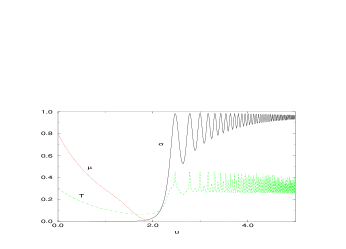
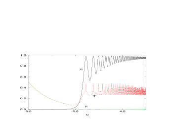
FIG. 2.: Evolution of $T$,$\mu$ and $\sigma$ as a function of $u$. Top figure is for 1st order transition. Bottom figure is for 2nd order phase transition

The order of the transition has a more noticeable effect on the spectrum of particles and antiparticles. If the system evolves in local thermal equilibrium with $\sigma=0$, then when $N^{\pm}(k,u)$ is plotted vs. $k_{\eta}=k\tau$ it is independent of $u$. A deviation from this result is an indication of the system going out of equilibrium. We find because of the “latent heat” released during a first order transition that the distortion of the spectrum is greatest in that case. (see Fig. 3). If one traverses the tricritical regime one finds results intermediate between the two cases displayed.

In local equilibrium with $\sigma=0$, $\epsilon=p\propto\tau^{-2}$ . Simulations, shown in Fig. 4 agree with this before the phase transition occurs. After the phase transition we find that the energy density oscillates around the true broken symmetry value discussed earlier, namely $\epsilon_{0}=-1/4\pi$. These oscillations would be damped if we included hard scattering effects [14]. The details of this calculation as well as a discussion of correlation functions and the effects of a bare mass will be presented elsewhere.

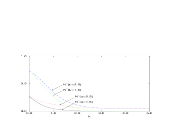
FIG. 3.: Evolution of $N_{\pm}$ as a function of $u$.Initial conditions are same as Fig. 2.The momentum displayed is $k_{\eta}=k\tau$

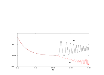
FIG. 4.: Evolution of the pressure and energy density as a function of $u$ .Initial conditions are same as Fig. 2.

We would like to thank Emil Mottola, Salman Habib and Dan Boyanovsky for discussions.

REFERENCES

[1] K. Rajagopal, hep-ph/0005101
[2]
D. Bailin and A. Love, Phys. Rept. 107, 325
(1984);
M. Alford, K. Rajagopal, and F. Wilczek, Phys. Lett. B 422, 247 (1998);
R. Rapp, T. Schäfer, E.V. Shuryak, and M. Velkovsky,
Phys. Rev. Lett. 81, 53 (1998);
J. Berges and K. Rajagopal, Nucl.Phys. B538,
215 (1999);
A. Barducci, R. Casalbuoni, G. Pettini and R. Gatto,
Phys. Rev. D 49,426 (1994);
M. A. Halasz, A.D. Jackson, R .E. Shrock, M.A. Stephanov
and J.J. M. Verbaarschot, Phys.Rev. D58, 096007 (1998);
M. A. Stephanov,Nucl.Phys.A642, 90 (1998);
R. Pisarski and D.H. Rischke, Phys.Rev.Lett. 83, 37 (1999)
D.T. Son, Phys.Rev. D59, 094019, (1999);
and references therein.
[3] A. Chodos, F. Cooper, W. Mao, H. Minakata, A. Singh
Phys.Rev. D61 (2000) 045011 hep-th/9905521.
[4]D.J. Gross and A. Neveu, Phys. Rev. D10 (1974) 3235.
[5] L. Jacobs, Phys. Rev.D 0 (1974) 3956.
U. Wolff, Phys. Lett. B157, 303 (1985).
[6] J. D. Bjorken, Phys. Rev. D27, 140
(1983); L. D. Landau, Izv. Akad. Nauk. SSSR (Ser. Fiz.)
17, 51 (1953);
F. Cooper, G. Frye and E. Schonberg, Phys. Rev. D11, 192
(1975).
[7] L. D. Landau and E.M. Lifschitz, Statistical Physics,
pp. 75 Second Edition, Addison - Wesley Publishing Company (1969).
[8]
F. Cooper J. M. Eisenberg,Y. Kluger,
E. Mottola, and B. Svetitsky,Phys. Rev. D48, 190 (1993);
[9] F. Cooper, Y.
Kluger and E. Mottola Phys. Rev. C54 3298 (1996) hep-ph/9604284.
M. Kennedy,J. Dawson and F. Cooper Phys.Rev.D54 2213, (1996).
hep-th/9603068
[10] Y. Kluger, J. M. Eisenberg, B. Svetitsky,
F. Cooper, and
E. Mottola, Phys. Rev. D45, 4659 (1992).
[11]D. Boyanovsky, D.-S. Lee, A. Singh
Phys.Rev. D48, 800 (1993), hep-th/9212083;
D. Boyanovsky, H.J. de Vega, R. Holman, D.S. Lee, A. Singh,
Phys.Rev. D51, 4419 (1995), hep-ph/9408214;
D. Boyanovsky, D. Cormier, H.J. de Vega, R. Holman, A. Singh, M. Srednicki,
Phys.Rev. D56,1939 (1997), hep-ph/970332.
[12] D.Boyanovsky, H.J. de Vega, R. Holman,
Phys.Rev.D51, 734 (1995), hep-ph/9401308.
[13] G. Aarts and J. Smit Phys.Rev.D61 (2000) 025002
hep-ph/9906538.
[14] J. Berges and J. Cox, hep-ph/0006160;B. Mihaila, F.
Cooper and J Dawson, hep-ph/0006254.