NONPERTURBATIVE CALCULATION OF SCATTERING AMPLITUDES

Abstract

A method for the nonperturbative calculation of scattering amplitudes and cross sections is discussed in the context of light-cone quantization. The Lanczos-based recursion method of Haydock is suggested for the computation of matrix elements of the resolvent for the light-cone Hamiltonian, from which the $T$-matrix can be constructed. The scattering of composite particles is handled by a generalization of a formulation given by Wick.

1 Introduction

Recently there has been a significant amount of progress in the nonperturbative calculation of bound-state properties in light-cone quantized field theories. [1, 2] Comparable progress in the calculation of scattering states has been lacking, although techniques have been proposed. [3] The ability to compute outcomes of scattering processes is not only of interest in its own right, but also useful for construction of renormalization conditions in bound-state calculations. [4] Here we consider a calculational scheme based on numerical approximations to resolvents [5] and on a generalization of a Hamiltonian formulation for the scattering of composites. [6]

The construction is done in terms of light-cone coordinates, where $t+z$ takes the role of time. [7, 1] This is not a necessary choice, but it does bring several advantages and makes immediate contact with work that uses these coordinates for bound-state problems. [1, 2] The advantages include a simple vacuum, well defined Fock-state expansions, and kinematical boosts. This last advantage is particularly important for the scattering of composites because one can compute the state of a composite particle in one frame and boost to other frames without again referencing the interaction.

The remainder of this paper is structured as follows: Section 2 contains a description of the notation used for light-cone coordinates and a formulation of two-body cross sections in terms of these coordinates. The key quantity in this formulation is a matrix element of a resolvent; a numerical method for its computation is discussed in Sec. 3 and applied to a nonrelativistic example in Sec. 4. An extension to the scattering of composites is given in Sec. 5. Finally, Sec. 6 provides a summary and indications of future work.

2 Cross Sections in Light-Cone Coordinates

We use the following notation for light-cone coordinates:

$$x^{\pm}=t\pm z\,,\;\;{\bf x}_{\perp}=(x,y)\,,$$ (1)

where $x^{+}$ is taken as the time variable. Momentum components are similarly defined

$$p^{\pm}=E\pm p_{z}\,,\;\;{\bf p}_{\perp}=(p_{x},p_{y})\,.$$ (2)

A dot product is then written as

$$p\cdot x=\frac{1}{2}(p^{+}x^{-}+p^{-}x^{+})-{\bf p}_{\perp}\cdot{\bf x}_{\perp}\,,$$ (3)

so that $p^{-}$ is conjugate to $x^{+}$ and is recognized as the light-cone energy. The other momentum components form the light-cone analog of the three-momentum

$$\underline{p}\equiv(p^{+},{\bf p}_{\perp})\,.$$ (4)

The evolution of a state is determined by the Hamiltonian ${\cal P}^{-}$; however, the term “light-cone Hamiltonian” is also used [8] for the combination

$$H_{\rm LC}=P^{+}{\cal P}^{-}\,,$$ (5)

where $P^{+}$ is the total momentum. The fundamental eigenvalue problem is

$$H_{\rm LC}|p\rangle=\frac{M^{2}+p_{\perp}^{2}}{p^{+}/P^{+}}|p\rangle\,,\;\;\underline{\cal P}|p\rangle=\underline{p}|p\rangle\,.$$ (6)

For two-body scattering $A+B\rightarrow C+D$, the center-of-mass cross section can be written [9]

$$\frac{d\sigma}{d\Omega}_{\rm cm}=\frac{1}{2E_{A}2E_{B}v_{\rm rel}}\frac{|\vec{p}_{C}||{\cal M}_{fi}|^{2}}{16\pi^{2}E_{\rm cm}}\,,$$ (7)

where $M_{fi}$ is the invariant amplitude extracted from the $S$ matrix

$$S_{fi}=\langle f|i\rangle+(2\pi)^{4}\delta^{(4)}(p_{f}-p_{i})i{\cal M}_{fi}\,,$$ (8)

with states normalized according to

$$\langle f|i\rangle=(16\pi^{3})^{2}p_{A}^{+}\delta(\underline{p}_{A}-\underline{p}_{C})p_{B}^{+}\delta(\underline{p}_{B}-\underline{p}_{D})\,.$$ (9)

The flux factors are determined by the current matrix element

$$\langle A|J^{0}|A\rangle=\frac{1}{2}\langle A|(J^{+}+J^{-})|A\rangle=2E_{A}\,,$$ (10)

with $E_{A}$ the energy of particle $A$. For fermions, the spinors are normalized by $\bar{u}u=2m$. From the optical theorem we also have

$$\sigma=\frac{2\,{\cal I}m{\cal M}_{ii}}{2E_{A}2E_{B}v_{\rm rel}}\,.$$ (11)

In the light-cone interaction picture [10] the invariant amplitude can be related to a matrix element of a $T$ operator. The $S$ matrix can be written as

$$S_{fi}=\langle f|U(x^{+},x_{0}^{+})|i\rangle=\langle f|i\rangle-2\pi iT_{fi}\delta(p_{f}^{-}-p_{i}^{-})\,,$$ (12)

with the $T$ operator defined by

$$T=V+V\frac{1}{p^{-}+i\epsilon-{\cal P}^{-}}V\,,$$ (13)

where

$${\cal P}^{-}={\cal P}_{0}^{-}+V\,.$$ (14)

On removal of the momentum conserving delta function

$$T_{fi}=t_{fi}\delta(\underline{p}_{f}-\underline{p}_{i})\,,$$ (15)

we obtain

$${\cal M}_{fi}=-\frac{1}{16\pi^{3}}t_{fi}\,.$$ (16)

We then need a means to compute $t_{fi}$. In particular, we need to handle matrix elements of the second term in $T$ which involve the resolvent $(p^{-}+i\epsilon-{\cal P}^{-})^{-1}$.

3 Recursion Method for Resolvents

We divide the matrix element of the $T$ operator into two pieces, the Born term and the resolvent term

$$T_{fi}=V_{fi}+T_{fi}^{(2)}\,,\;\;T_{fi}^{(2)}\equiv\langle f|V\frac{1}{p^{-}+i\epsilon-{\cal P}^{-}}V|i\rangle\,.$$ (17)

To the latter we apply the recursion method developed by Haydock [5] in the context of condensed matter physics. This method is based on the Lanczos diagonalization algorithm [11] which converts the original Hamiltonian operator into an approximate tridiagonal representation. The tridiagonal form is easily inverted to yield the resolvent.

Define an initial vector $|u_{1}\rangle=cV|i\rangle$, with $c$ a normalization constant, and carry out Lanczos recursions [11]

$$b_{1} = 0\,,\;\;a_{n}=\langle u_{n}|{\cal P}^{-}|u_{n}\rangle\,,\;\;\langle u_{n}|u_{n}\rangle=1\,,$$

$$b_{n+1}|u_{n+1}\rangle = {\cal P}^{-}|u_{n+1}\rangle-a_{n}|u_{n}\rangle-b_{n}|u_{n-1}\rangle\,.$$ (18)

Although this could in principle be done analytically, the usual approach is to begin with a large but sparse matrix representation for ${\cal P}^{-}$ in a Fock basis. A standard way of constructing such a representation is discrete light-cone quantization (DLCQ). [8, 1] The vectors $|u_{n}\rangle$ provide an orthonormal basis in which ${\cal P}^{-}$ has the tridiagonal representation

$${\cal P}^{-}\rightarrow\left(\begin{array}[]{llllll}a_{1}&b_{2}&0&0&0&\ldots\\ b_{2}&a_{2}&b_{3}&0&0&\ldots\\ 0&b_{3}&a_{3}&b_{4}&0&\ldots\\ 0&0&b_{4}&.&.&\ldots\\ 0&0&0&.&.&\ldots\\ .&.&.&.&.&\ldots\end{array}\right)\equiv A\,,$$ (19)

and the forward matrix element of the resolvent is approximated by the upper left matrix element of the inverse

$$T_{ii}^{(2)}\simeq\frac{1}{c^{2}}\left\{[(p_{i}^{-}+i\epsilon)I-A]^{-1}\right\}_{1,1}\,.$$ (20)

Non-forward matrix elements can be obtained by using the block Lanczos procedure in place of the ordinary one described above. [12]

Unfortunately, the discrete nature of the calculation does not allow this finite matrix representation to be useful in all respects. In the limit of $\epsilon\rightarrow 0$, the imaginary part of this approximation to $T_{ii}^{(2)}$ will contain only delta functions at the discrete eigenvalues of the finite matrix approximation $A$. To properly model the contribution from the continuum, an extension must be made. This can be done in terms of a continued fraction representation

$$c^{2}T_{ii}^{(2)}=\frac{1}{p_{i}^{-}+i\epsilon-a_{1}-\frac{b_{2}^{2}}{p_{i}^{-}+i\epsilon-a_{2}-\frac{b_{3}^{2}}{p_{i}^{-}+i\epsilon-a_{3}-\cdots}}}\,,$$ (21)

by replacing the last level with a terminator, a model for an infinite fraction. [13]

A model can be generated in various ways; however, a logical choice in the present situation is to use the second Born approximation as a generator. The matrix element of the resolvent for the free Hamiltonian

$$\langle i|V\frac{1}{p^{-}+i\epsilon-{\cal P}_{0}^{-}}V|i\rangle$$ (22)

is computed exactly and then in continued fraction form by iterating with ${\cal P}_{0}^{-}$ an equal number of times. The exact form dictates the structure of the remaining infinite fraction, which is used as a terminator for the full resolvent.

4 Nonrelativistic Example

As an example of how the terminated recursion method works, we consider nonrelativistic S-wave scattering from an exponential potential. This is a common choice for testing numerical methods for scattering problems because it has an exact solution.

The partial wave expansion for the $T$-matrix is

$$\langle\vec{k}^{\,\prime}|T(E)|\vec{k}\rangle=\frac{1}{2\pi^{2}}\sum_{l}(2l+1)T_{l}(k^{\prime},k;E)P_{l}(\hat{k}^{\,\prime}\cdot\hat{k})\,,$$ (23)

where

$$T_{l}(k^{\prime},k;E) = \int dru_{k^{\prime}l}(r)V(r)u_{kl}(r)$$ (25)

$$+\int dru_{k^{\prime}l}(r)V(r)\frac{1}{E+i\epsilon-H_{l}}V(r)u_{kl}(r)$$

and

$$u_{kl}(r)=rj_{l}(kr)\,,\;\;H_{l}=-\frac{1}{2m}\frac{d^{2}}{dr^{2}}+\frac{l(l+1)}{2mr^{2}}+V(r)\,.$$ (26)

The partial wave contribution $T_{l}$ is related to the phase shift $\delta_{l}$ by

$$T_{l}(k,k;k^{2}/2m)=-\frac{1}{2mk}e^{i\delta_{l}}\sin\delta_{l}\;\;\mbox{or}\;\;\tan\delta_{l}=\frac{{\cal I}mT_{l}}{{\cal R}eT_{l}}\,.$$ (27)

For S-wave scattering of a particle of mass $m$ from $V(r)=-e^{-r/a}/ma^{2}$
the exact solution is [14]

$$\delta_{0}(k)=\mbox{Arg}(J_{2ika}(2\sqrt{2})\Gamma(1+2ka))-2ka\ln\sqrt{2}\,.$$ (28)

To solve this problem numerically,  we introduce a discrete approximation with $M$ interior points between $r=0$ and a radial cutoff $R$. The step size is

$$\Delta r=\frac{R}{M+1}\,.$$ (29)

Integrals are approximated by the trapezoidal rule, and derivative operators by finite differences. The radial cutoff is kept larger than $2\pi/k$ in order to include one complete wavelength at the chosen energy. The terminator for the recursion is generated from the second Born approximation

$$T_{l}^{(2)}\simeq\int drdr^{\prime}u_{k^{\prime}l}(r^{\prime})V(r^{\prime})g_{El}^{(0)}(r^{\prime},r)V(r)u_{kl}(r)\,,$$ (30)

where

$$g_{El}^{(0)}(r^{\prime},r)=-\frac{mi\kappa}{2\pi}rr^{\prime}j_{l}(\kappa r_{<})h_{l}^{+}(\kappa r_{>})$$ (31)

and $\kappa=\sqrt{2mE}$.

Figure 1 displays the results of calculations done for $k=0.25/a$, $R=30a>2\pi/k\simeq 25a$, and $M=49$, 99, 199, 399, and 799. They show good convergence properties. More importantly, they show that the imaginary part of the $T$-matrix element is calculated reliably.

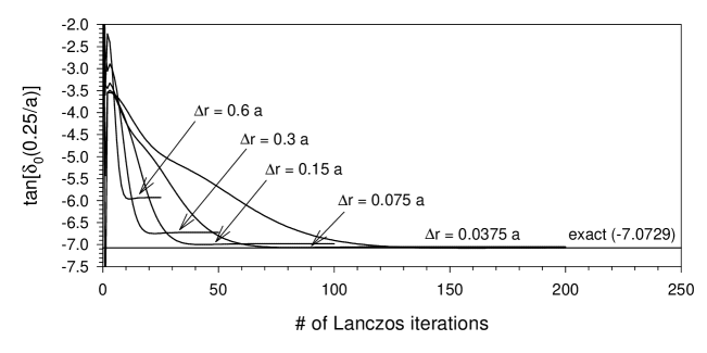
Figure 1: Phase shift for S-wave scattering from an exponential potential, as computed by the recursion method with termination based on the second Born approximation. $\Delta r$ is the spacing used in trapezoidal approximations to the integral expression for the partial-wave $T$ matrix element.

5 Scattering of Composites

The formulation in Sec. 2 assumes implicitly that the particles involved in the scattering process are elementary. In a field-theoretic setting this is not typically the case for a nonperturbative calculation. The particles $A$, $B$, $C$, and $D$ can be themselves complicated bound states of the full Hamiltonian. It is then difficult to determine the nature of the interaction $V$ that appears in the $T$ operator.

To construct the form of the $T$ operator in this case, we generalize a construction given by Wick [6] to compute the $S$ matrix

$$S_{AB\rightarrow CD}=\langle CD-|AB+\rangle$$ (32)

from scattering eigenstates of the light-cone Hamiltonian $H_{\rm LC}$. Let $A^{\dagger}$ and $B^{\dagger}$ create one-particle solutions from the Fock vacuum $|0\rangle$, so that

$$|A\rangle=A^{\dagger}|0\rangle\,,\;\;H_{\rm LC}|A\rangle=\frac{m_{A}^{2}+p_{A\perp}^{2}}{p_{A}^{+}/P^{+}}|A\rangle\,.$$ (33)

The two-particle scattering eigenstates of $H_{\rm LC}$ are then

$$|AB\pm\rangle=B^{\dagger}|A\rangle+\frac{1}{s_{AB}\pm i\epsilon-H_{\rm LC}}V_{B}|A\rangle\,,$$ (34)

where

$$V_{B}\equiv[H_{\rm LC},B^{\dagger}]-\frac{m_{B}^{2}+p_{B\perp}^{2}}{p_{B}^{+}/P^{+}}B^{\dagger}$$ (35)

and

$$s_{AB}=\frac{m_{A}^{2}+p_{A\perp}^{2}}{p_{A}^{+}/P^{+}}+\frac{m_{B}^{2}+p_{B\perp}^{2}}{p_{B}^{+}/P^{+}}$$ (36)

is the invariant mass of the scattering state and the Mandelstam $s$ of the scattering process. The definition of $V_{B}$ is chosen to ensure that

$$H_{\rm LC}|AB\pm\rangle=s_{AB}|AB\pm\rangle\,.$$ (37)

The $T$ operator is constructed by reducing the $S$ matrix to

$$S_{AB\rightarrow CD}=\delta_{CD,AB}-2\pi i\delta(s_{AB}-s_{CD})T_{{\rm LC}fi}\,.$$ (38)

We find

$$T_{{\rm LC}fi}=P^{+}T_{fi}=\langle CD-|V_{B}|A\rangle\,,$$ (39)

which can be expanded as

$$P^{+}T_{fi}=\langle C|V_{D}^{\dagger}\frac{1}{s_{AB}+i\epsilon-H_{\rm LC}}V_{B}|A\rangle+\langle C|DV_{B}|A\rangle\,,$$ (40)

with

$$\langle C|DV_{B}|A\rangle = \langle C|V_{B}\frac{1}{s_{AB}-\frac{m_{B}^{2}+p_{B\perp}^{2}}{p_{B}^{+}/P^{+}}-\frac{m_{D}^{2}+p_{D\perp}^{2}}{p_{D}^{+}/P^{+}}-H_{\rm LC}}V_{D}^{\dagger}|A\rangle$$ (41)

$$+\langle C|[D,V_{B}]|A\rangle\,.$$

The first term in (40) can be interpreted as a direct scattering of $B$ by $A$. The first term in (41) is the crossed contribution, where $D$ is produced before $B$ is absorbed. The second term in (41) is a generalized seagull contribution, which did not appear in Wick’s formalism. [6]

To use these expressions efficiently, $\langle C|DV_{B}|A\rangle$ should be computed explicitly rather than work with the decomposition into crossed and seagull terms. This is because the decomposition introduces an inverse of the Hamiltonian. The inverse is unavoidable for the direct term, and here one would apply the recursion method discussed in the previous sections. For both terms one needs the action of $V_{B}$ on the one-particle state $|A\rangle$.

6 Concluding Remarks

A method for the nonperturbative calculation of cross sections has been presented in the context of light-cone quantized field theories. The key expression is (40), where the light-cone $T$ matrix is given in terms of known operators and composite-particle eigenstates. The terminated recursion technique of Haydock [5] is to be used to handle the inverse of the light-cone Hamiltonian. Work on an application to a simple model [2] is in progress. One direction to consider for possible improvements to the method is to explore variational formulations analogous to the Schwinger and Kohn variational principles [15] used in nonrelativistic scattering.

References

References

- [1] For a review, see S.J. Brodsky, H.-C. Pauli, and S.S. Pinsky, Phys. Rep. 301, 299 (1997).
- [2] S.J. Brodsky, J.R. Hiller, and G. McCartor, Phys. Rev. D 58, 025005 (1998); 60, 054506 (1999); J.R. Hiller, in the proceedings of the TJNAF workshop on the Transition from Low to High Q Form Factors, Athens, GA, September 17, 1999, p. 193, hep-ph/9909471; J.R. Hiller, to appear in the proceedings of the CSSM Workshop on Light-Cone QCD and Nonperturbative Hadron Physics, Adelaide, Australia, December 13-21, 1999, hep-ph/0002222.
- [3] J.R. Hiller, Phys. Rev. D 43, 2418 (1991); H. Kröger, Phys. Rep. 210, 45 (1992); C.-R. Ji and Y. Surya, Phys. Rev. D 46, 3565 (1992); M.G. Fuda and Y. Zhang, Phys. Rev. C 51, 23 (1995). For a lattice gauge theory approach, see M. Lüscher, Nucl. Phys. B 354, 531 (1991).
- [4] J.R. Hiller and S.J. Brodsky, Phys. Rev. D 59, 016006 (1999).
- [5] R. Haydock, in Solid State Physics, eds. H. Ehrenreich, F. Seitz, and D. Turnbull (Academic, New York, 1980), Vol. 35, p. 283.
- [6] G.C. Wick, Rev. Mod. Phys. 27, 339 (1955).
- [7] P.A.M. Dirac, Rev. Mod. Phys. 21, 392 (1949).
- [8] H.-C. Pauli and S.J. Brodsky, Phys. Rev. D 32, 1993 (1985); 32, 2001 (1985).
- [9] M.E. Peskin and D.V. Schroeder, An Introduction to Quantum Field Theory, (Addison-Wesley, Reading, MA, 1995).
- [10] M.G. Fuda, Phys. Rev. D 44, 1880 (1991).
- [11] C. Lanczos, J. Res. Nat. Bur. Stand. 45, 255 (1950); J. Cullum and R.A. Willoughby, in Large-Scale Eigenvalue Problems, eds. J. Cullum and R.A. Willoughby, Math. Stud. 127 (Elsevier, Amsterdam, 1986), p. 193.
- [12] C.M.M. Nex, Comput. Phys. Commun. 53, 141 (1989); W. Yang and W.H. Miller, J. Chem. Phys. 91, 3504 (1989); H.D. Meyer and S. Pal, J. Chem. Phys. 91, 6195 (1989); T.J. Godin and R. Haydock, Comput. Phys. Commun. 64, 123 (1991).
- [13] R. Haydock and C.M.M. Nex, J. Phys. C 18, 2235 (1985).
- [14] P.M. Morse and H. Feshbach, Methods of Theoretical Physics, Vol. II, (McGraw-Hill, New York, 1953), p. 1687; M. Sebhata and W.E. Gettys, Comput. Phys. 3, 65 (1989).
- [15] J. Schwinger, Phys. Rev. 72, 742 (1947); W. Kohn, Phys. Rev. 74, 1763 (1948); C. Duneczky and R.E. Wyatt, J. Chem. Phys. 89, 1448 (1988); H.-D. Meyer, J. Horáček, and L.S. Cederbaum, Phys. Rev. A 43, 3587 (1991).