Logarithmic SUSY electroweak effects on four-fermion processes at TeV energies

Abstract

We compute the MSSM one-loop contributions to the asymptotic energy behaviour of fermion-antifermion pair production at future lepton-antilepton colliders. Besides the conventional logarithms of Renormalization Group origin, extra SUSY linear logarithmic terms appear of ”Sudakov-type”. In the TeV range their overall effect on a variety of observables can be quite relevant and drastically different from that obtained in the SM case.

I Introduction.

In recent papers [1], [2], the effects of one-loop diagrams on fermion-antifermion pair production at future lepton-antilepton colliders were computed in the SM for both massless [1] and massive (in practice, bottom production) [2] fermions. As a result of that calculation it was found that, in the high energy region, contributions arise that are both of linear and of quadratic logarithmic kind in the c.m. energy, but are not of Renormalization Group (RG) origin. For this reason they were called [3] ”of Sudakov-type”, [4], although the theoretical mechanism that generates them is not, rigorously speaking, of infrared origin, as exaustively discussed in following articles [5]. In this paper, we shall retain the original ”Sudakov-type” notation, but one might call these terms e.g. ”not of RG origin” to avoid theoretical confusion.

As a by product of our computations, it was also stressed in [2] that, in the special case of bottom-antibottom production, extra terms appear that are ”of Sudakov-type” and also quadratic in the top mass, a situation that reminds that met at the $Z$-peak in the calculation of the partial $Z$ width into $b\bar{b}$. Neglecting these terms would produce a serious theoretical mistake in the case of certain observables, particularly the $b\bar{b}$ cross section, and in principle (for very high lumonisity) also in the $b\bar{b}$ longitudinal polarization asymmetry.

When the c.m. energy crosses the typical TeV limit, the relative effects of the ”Sudakov-type” logarithms begin to rise well beyond the (tolerable) few percent threshold, making the validity of a one-loop approximation not always obvious, depending on the chosen observable. In particular, hadronic production seems to be in a critical shape, as discussed in [5]. These conclusions are quite different from those that would be obtained if only the RG linear asymptotic logarithms were retained. In that case, the smooth relative effect would remain systematically under control at TeV energies, not generating special theoretical diseases. On the contrary, in the ”Sudakov” case a subtle mechanism of opposite linear and quadratic logarithms contributions often appears that makes the overall effect less controlable. Thus, neglecting the non RG asymptotic effects in the considered processes would certainly be a theoretical disaster.

The aim of this paper is that of investigating whether similar conclusions can be drawn when one works in the framework of a supersymmetric extension of the SM. In particular, although the same analysis could be performed in a more general case, we shall fix our attention here on the simplest minimal SUSY model (MSSM) [6]. We shall be motivated in this search by (at least) two qualitative reasons. These are a consequence of the results obtained in Ref.[1], showing that in some cases the relative size of the effects becomes larger than the expected experimental accuracy. If SUSY extra diagrams increased this value, their rigorous inclusion at one-loop would be essential e.g. for a test of the theory if SUSY partners were discovered. But even if direct production were still lacking for some special ”heavy” SUSY particles (e.g. neutralinos), a large virtual effect in some observable might be, in principle, detectable. In this spirit, we shall proceed in this paper as follows. We shall assume that SUSY has been at least partially detected, and that for all the masses of the model a ”natural” mechanism [7] exists that confines their values below the TeV limit (in practice, they might roughly be of the same size as the top mass). In this spirit, the c.m. energy region beyond one TeV can be considered as ”nearly” asymptotic. This means that we shall have in our minds, more than the future 500 GeV Linear Collider (LC) [8] case, that of the next CERN Compact Linear Collider (CLIC) [9], supposed to be working at energies between 3 and 5 TeV. With due care, though, we feel that a number of our conclusions might well be extrapolated to the LC situation, as illustrated in the original Ref.[1].

In Section II of this paper we shall review the various MSSM diagrams that give rise to ”Sudakov” logarithms and discuss the analogies and the differences with respect to the SM. We shall discuss separately the various contributions both in the massless case and in that of $b\bar{b}$ production (the case of top production, that requires a modification of the adopted theoretical scheme, will be treated separately in a forthcoming paper). For final bottom, we shall show that the overall logarithmic genuine SUSY contributions that are also quadratic in the top mass enhance the corresponding SM ones. Moreover, there appear terms that are quadratic in the bottom mass and are multiplied by $\tan^{2}\beta$, which could also be sizeable for very large values of $\tan^{2}\beta$. The obtained expressions of the various observables will be shown in Section III, and the features of the MSSM relative effects will be displayed in several Figures. It will appear that the MSSM logarithmic effects are drastically different from those of the SM, and again quite different from those obtained in the pure RG approximation. The expectable validity of a logarithmic parametrization will be discussed in the final Section IV, with special emphasis on the CLIC energy region but also on the LC case. The possibility of a relatively simple parametrization to be used in the TeV energy range will be also qualitatively motivated. Finally, a short Appendix will contain the detailed asymptotic logarithmic contributions from various diagrams to the four gauge-invariant functions that in our approach generate all the observable quantities of the considered process at the electroweak one loop.

II MSSM diagrams generating asymptotic logarithms

The theoretical analysis of this paper is based on the use of the so called ”$Z$-peak-subtracted” representation, which has been illustrated in several previous references [10] and was conveniently used to describe the process of electron-positron annihilation into a final fermion ($f$) antifermion $\bar{f}$, that can be either a lepton-antilepton or a ”light” ($u,d,s,c,b$) quark-antiquark pair. For what concerns the genuine electroweak sector of the process, all the relevant information is provided by four gauge-invariant functions of $q^{2}$ and $\theta$ (the squared c.m. energy and scattering angle) that are called $\tilde{\Delta}_{\alpha lf}$, $R_{lf}$, $V^{\gamma Z}_{lf}$, $V^{Z\gamma}_{lf}$ and describe one-loop transitions of various Lorentz structure (photon-photon, $Z$-$Z$, photon-$Z$ and $Z$-photon respectively). These functions vanish by construction at $q^{2}=0$ ($\tilde{\Delta}_{\alpha}$) and $q^{2}$= $M_{Z}^{2}$ (the other three quantities) respectively and are ultraviolet finite. They enter the theoretical expression of the various cross sections and asymmetries in a way that is summarized in the Appendix B of Ref.[1], and we will not insist on their properties here.

At one loop, the previous four gauge-invariant functions receive contributions from diagrams of self-energy, vertex and box type. Self-energy diagrams with a small addition of the ”pinch” part of the $WW$ vertex generate asymptotically logarithms of the c.m. energy in agreement with the Renormalization Group (RG) treatment. Extra logarithms of ”pseudo-Sudakov” type (we follow the original denomination of Degrassi and Sirlin [11], whose description of four-fermion processes has been adopted in our work) arise in the SM from two kinds of diagrams. Vertices with one or two internal $W^{\prime}s$ or one internal $Z$ generate both linear and quadratic logarithms; boxes with either $W^{\prime}s$ or $Z^{\prime}s$ do the same. For massless fermions, there are no other types of logarithms. However, for final bottom-antibottom production, vertex diagrams produce extra linear logarithms that are also quadratic in the top mass, and cannot be neglected. All these results can be found in [1], [2]; for completeness we have also written the same type of terms quadratic in the bottom mass although they are numerically negligible.

When one moves to the MSSM, the situation becomes, at least for what concerns this special topics, relatively simpler. In fact, one discovers immediately that box diagrams with internal SUSY partners do not generate asymptotic logarithms. This feature, that is quite different from the SM one, is due to the different spin structure of the fermion-fermion-scalar couplings which arise in SUSY and replace the fermion-fermion-vector couplings arising in SM. As a consequence, when the energy increases, the SUSY box contribution vanish as an inverse power of $q^{2}$. Thus only self-energies and vertices must be considered. Self-energies will generate the RG logarithmic behaviour. Summing the various bubbles involving SUSY partners ($\tilde{f}$, $\chi^{\pm}$, $\chi^{0}$), Higgses ($A^{0}$, $H^{0}$, $h^{0}$), and Goldstones, we obtain the self-energy contributions to the four functions $\tilde{\Delta}_{\alpha lf}$, $R_{lf}$, $V^{\gamma Z}_{lf}$, $V^{Z\gamma}_{lf}$ given in the Appendix. Using the relations between these contributions and the expressions giving the running of $g_{1}$, $g_{2}$, $s^{2}_{W}$ established in Ref.[1], we have checked that our result agrees with the running quoted in the literature [12] for both the SM and the MSSM cases.

For vertices, the analysis is, to our knowledge, new and, in our opinion, interesting. First, and again because of the absence of helicity conserving fermion-fermion-vector couplings, in SUSY there is no helicity structure analogue to the one brought by the SM ($WWf$) triangle and then no quadratic logarithmic contribution. However there appears linear logarithmic contributions called of ”Sudakov-type” because they are not universal and do not contribute to RG. For massless fermions, they are generated by the diagrams that involve chargino(s) or neutralino(s) together with sfermions exchanges as shown in Fig.1; the related effects on the four functions are given in the Appendix. They can be compared with the corresponding SM effects computed in Ref.[1], Section 2.3.

A special discussion is due to the case of final $b\bar{b}$ production. Here to the previous SUSY diagrams one must add the contributions from the MSSM Higgses, exactly like in the SM case. So we shall have both contributions of chargino/neutralino-sfermion origin, see Fig.1 (denoted by a symbol $\chi$), and of Higgs origin, see Fig.2 (denoted by a symbol $H$). Note that, being interested in the additional contribution brought by SUSY, to be later on added to the SM contribution in order to get the full MSSM one, in the Higgs part ($H$), we write the total MSSM Higgs contribution minus the SM Higgs contribution.

For the purposes of the following discussion it is convenient to write the effects of the previous diagrams, rather than on the gauge-invariant subtracted functions, on the photon and $Z$ vertices $\Gamma_{\mu}^{\gamma}$, $\Gamma_{\mu}^{Z}$, defined in a conventional way [1],[11]. One easily finds first the $\chi$ contribution and secondly the ($H$) contribution:

$$\Gamma^{\gamma}_{\mu}(\chi) \to -({e\alpha\over 48\pi M^{2}_{W}s^{2}_{W}})lnq^{2}[m^{2}_{t}(1+{1\over tan^{2}\beta})(\gamma^{\mu}P_{L})$$ (2)

$$+m^{2}_{b}(1+tan^{2}\beta)\{(\gamma^{\mu}P_{L})+2(\gamma^{\mu}P_{R})\}]$$

$$\Gamma^{Z}_{\mu}(\chi) \to -({e\alpha\over 48\pi M^{2}_{W}s^{3}_{W}c_{W}})lnq^{2}[({3\over 2}-s^{2}_{W})m^{2}_{t}(1+cot^{2}\beta)(\gamma^{\mu}P_{L})$$ (4)

$$+m^{2}_{b}(1+tan^{2}\beta)\{({3\over 2}-s^{2}_{W})(\gamma^{\mu}P_{L})-2s^{2}_{W}(\gamma^{\mu}P_{R})\}]$$

$$\Gamma^{\gamma}_{\mu}(H) \to -({e\alpha\over 48\pi M^{2}_{W}s^{2}_{W}})lnq^{2}[m^{2}_{t}cot^{2}\beta(\gamma^{\mu}P_{L})+m^{2}_{b}tan^{2}\beta\{(\gamma^{\mu}P_{L})+2(\gamma^{\mu}P_{R})\}]$$ (5)

$$\Gamma^{Z}_{\mu}(H) \to -({e\alpha\over 48\pi M^{2}_{W}s^{3}_{W}c_{W}})lnq^{2}[({3\over 2}-s^{2}_{W})m^{2}_{t}cot^{2}\beta(\gamma^{\mu}P_{L})$$ (7)

$$+m^{2}_{b}tan^{2}\beta)\{({3\over 2}-s^{2}_{W})(\gamma^{\mu}P_{L})-2s_{W}^{2}(\gamma^{\mu}P_{R})\}]$$

where $P_{L,R}=(1\mp\gamma^{5})/2$.

In the previous equations, we have retained not only the terms proportional to $m_{t}^{2}$ and to $m_{b}^{2}tg^{2}\beta$, as usually done (the latter ones become competitive for large $tg\beta$ values), but also those simply proportional to $m_{b}^{2}$, that are usually discarded. Note that we did not retain SUSY masses inside the logarithm, being for the moment only interested in the asymptotic energy limit. In principle, we could use a common reference mass M and discard constant terms in the formulae. In fact, these possible constants will be thoroughly discussed in the final part of this paper. Thus, all the (bottom, top) mass terms contributing the asymptotic logarithms has been retained and, as one sees, they are not vanishing and in principle numerically relevant, as one could easily verify by computing their separate effects on the various observables. This is, in principle, no surprise since the corresponding terms in the SM were also, as we said, not negligible. To be more precise, we write the ”massive” SM vertices, that were computed in Ref.[2], simply adding the terms proportional to $m_{b}^{2}$ that were neglected in that paper, obtaining the expressions:

$$\Gamma^{\gamma}_{\mu}(SM,~{}massive) \to -({e\alpha\over 48\pi M^{2}_{W}s^{2}_{W}})lnq^{2}[m^{2}_{t}(\gamma^{\mu}P_{L})+m^{2}_{b}(\gamma^{\mu}P_{R})]$$ (9)

$$-({e\alpha m^{2}_{b}\over 48\pi M^{2}_{W}s^{2}_{W}})lnq^{2}[(\gamma^{\mu}P_{L})+(\gamma^{\mu}P_{R})]$$

$$\Gamma^{Z}_{\mu}(SM,~{}massive) \to -({e\alpha\over 48\pi M^{2}_{W}s^{3}_{W}c_{W}})lnq^{2}[({3\over 2}-s^{2}_{W})m^{2}_{t}(\gamma^{\mu}P_{L})-s^{2}_{W}m^{2}_{b}(\gamma^{\mu}P_{R})]$$ (11)

$$-({e\alpha m^{2}_{b}\over 48\pi M^{2}_{W}s^{3}_{W}c_{W}})lnq^{2}[({3\over 2}-s^{2}_{W})(\gamma^{\mu}P_{L})-s^{2}_{W}(\gamma^{\mu}P_{R})]$$

and adding Eqs.(2)-(7) we obtain the total massive terms in the MSSM:

$$\Gamma^{\gamma}_{\mu}(MSSM,~{}massive) \to -({e\alpha\over 24\pi M^{2}_{W}s^{2}_{W}})ln({q^{2}\over m^{2}_{t}})[m^{2}_{t}(1+cot^{2}\beta)(\gamma^{\mu}P_{L})$$ (13)

$$+m^{2}_{b}(1+tan^{2}\beta)\{(\gamma^{\mu}P_{L})+2(\gamma^{\mu}P_{R})\}]$$

$$\Gamma^{Z}_{\mu}(MSSM,~{}massive) \to -({e\alpha\over 24\pi M^{2}_{W}s^{3}_{W}c_{W}})ln({q^{2}\over m^{2}_{t}})[m^{2}_{t}({3\over 2}-s^{2}_{W})(1+cot^{2}\beta)(\gamma^{\mu}P_{L})$$ (15)

$$+m^{2}_{b}(1+tan^{2}\beta)\{({3\over 2}-s^{2}_{W})(\gamma^{\mu}P_{L})-2s^{2}_{W}(\gamma^{\mu}P_{R})\}]$$

Notices that there exists a very simple practical rule to move from the SM to the MSSM for what concerns the asymptotic mass effects. One just multiplies the $m^{2}_{t}$ term of the SM by $2(1+cot^{2}\beta)$ and the $m^{2}_{b}$ one by $2(1+tan^{2}\beta)$ . This will have practical consequences that will be fully illustrated in the following Section III.

III Asymptotic expressions of the observables.

After this preliminary discussion, we are now ready to compute the dominant asymptotic logarithmic terms in the various observables. For the massless SUSY partner sector of the MSSM, they will only be produced by self-energies (the RG component) and by the vertices with $\chi^{\pm},\chi^{0}$ shown in Fig.1, computed for massless fermions (the ”Sudakov-type” terms). For the massive sector they will be produced both by ($\chi$) mass effects of Fig.1 and by ($H$) mass effects of Fig.2 as discussed in the preceding Section. Using the standard couplings conventions [14] leads to expressions for the photon and $Z$ vertices that can be easily ”projected” on the four gauge-invariant functions. From the equations given in the Appendix B of Ref.[1] one can then derive the effect on various observables. To save space and time, we omit these intermediate steps and give directly the latter expressions in the following equations. We have considered here both the case of unpolarized production of the five ”light” quarks and leptons and that of polarized initial electron beams. The latter case would lead to the observation of a number of longitudinal polarization asymmetries, whose properties have been exhaustively discussed elsewhere [15]. We have considered for final quarks the overall hadronic production (symbol $5$) and that of the separate bottom (symbol $b$), that exhibits interesting features that will be discussed. The overall results shown in the following equations also include the SM effects previously computed [1], [2].

The various terms are grouped in the following order: first the RG(SM) with the mass scale $\mu$, followed by the linear and quadratic Sudakov (SM, W) terms, the linear and quadratic Sudakov (SM, Z) terms and finally, in the case of hadronic observables, the linear Sudakov term arising from the quadratic $m^{2}_{t}$ contribution; then, in bold face, the SUSY contributions, first the RG (SUSY) term with the mass scale $\mu$, then the linear Sudakov (SUSY) term (scaled by the common mass $M$), the linear massless Sudakov (SUSY) term arising from the quadratic $m^{2}_{t}$ contribution (scaled by a common mass $M^{\prime}$) and in curly brackets the same term to which the $m_{b}^{2}\tan^{2}\beta$ contribution is added for $\tan\beta=40$. This was done in order to show precisely the difference between the total SM prediction and the total SUSY part.

$$\sigma_{\mu} = \sigma^{B}_{\mu}[1+{\alpha\over 4\pi}\{(7.72\,N-20.58)\,ln{q^{2}\over\mu^{2}}+(35.27\,ln{q^{2}\over M^{2}_{W}}-4.59\,ln^{2}{q^{2}\over M^{2}_{W}})$$ (18)

$$+(4.79\,ln{q^{2}\over M^{2}_{Z}}-1.43\,ln^{2}{q^{2}\over M^{2}_{Z}})$$

$$+{\bf(3.86\,N+7.75)\,ln{q^{2}\over\mu^{2}}-10.02\,ln{q^{2}\over M^{2}}}\}]$$

$$A_{FB,\mu} = A^{B}_{FB,\mu}+{\alpha\over 4\pi}\{(0.54\,N-5.90)\,ln{q^{2}\over\mu^{2}}+(10.19\,ln{q^{2}\over M^{2}_{W}}-0.08\,ln^{2}{q^{2}\over M^{2}_{W}})$$ (21)

$$+(1.25\,ln{q^{2}\over M^{2}_{Z}}-0.004\,ln^{2}{q^{2}\over M^{2}_{Z}})$$

$$+{\bf(0.27\,N+1.57)\,ln{q^{2}\over\mu^{2}}-0.079\,ln{q^{2}\over M^{2}}}\}$$

$$A_{LR,\mu} = A^{B}_{LR,\mu}+{\alpha\over 4\pi}\{(1.82\,N-19.79)\,ln{q^{2}\over\mu^{2}}+(30.76\,ln{q^{2}\over M^{2}_{W}}-3.52\,ln^{2}{q^{2}\over M^{2}_{W}})$$ (24)

$$+(0.78\,ln{q^{2}\over M^{2}_{Z}}-0.17\,ln^{2}{q^{2}\over M^{2}_{Z}})$$

$$+{\bf(0.91\,N+5.25)\,ln{q^{2}\over\mu^{2}}-3.69\,ln{q^{2}\over M^{2}}}\}.$$

$$\sigma_{5} = \sigma^{B}_{5}[1+{\alpha\over 4\pi}\{(9.88\,N-42.66)\,ln{q^{2}\over\mu^{2}}+(46.58\,ln{q^{2}\over M^{2}_{W}}-6.30\,ln^{2}{q^{2}\over M^{2}_{W}})$$ (27)

$$+(7.25\,ln{q^{2}\over M^{2}_{Z}}-2.03\,ln^{2}{q^{2}\over M^{2}_{Z}})-~{}1.21\ln{q^{2}\over m^{2}_{t}}$$

$$+{\bf(4.94\,N+13.66)\,ln{q^{2}\over\mu^{2}}-10.99\,ln{q^{2}\over M^{2}}-3.65\{-5.21\}\ln{q^{2}\over M^{\prime 2}}}\}$$

$$A_{LR,5} = A^{0}_{LR,5}+{\alpha\over 4\pi}\{(2.11N-22.95)\ln{q^{2}\over\mu^{2}}$$ (31)

$$+(24.07\ln{q^{2}\over M^{2}_{W}}-3.12\ln^{2}{q^{2}\over M^{2}_{W}})$$

$$+(1.63\ln{q^{2}\over M^{2}_{Z}}-0.55\ln^{2}{q^{2}\over M^{2}_{Z}})-~{}0.53\ln{q^{2}\over m^{2}_{t}}$$

$$+{\bf(1.05\,N+6.09)\,ln{q^{2}\over\mu^{2}}-3.63\,ln{q^{2}\over M^{2}}-1.60\{+0.44\}\ln{q^{2}\over M^{\prime 2}}}\}\ ,$$

$$\sigma_{b} = \sigma^{B}_{b}\{1+{\alpha\over 4\pi}\{(10.88N-53.82)\ln{q^{2}\over\mu^{2}}+(76.75\ln{q^{2}\over M^{2}_{W}}-7.10\ln^{2}{q^{2}\over M^{2}_{W}})$$ (34)

$$+(11.98\ln{q^{2}\over M^{2}_{Z}}-2.45\ln^{2}{q^{2}\over M^{2}_{Z}})-~{}8.42\ln{q^{2}\over m^{2}_{t}}$$

$$+{\bf(5.44\,N+16.61)\,ln{q^{2}\over\mu^{2}}-11.82\,ln{q^{2}\over M^{2}}-25.3\{-36.0\}\ln{q^{2}\over M^{\prime 2}}}\}\ ,$$

$$A_{FB,b} = A^{B}_{FB,b}+{\alpha\over 4\pi}\{(0.56N-6.13)\ln{q^{2}\over\mu^{2}}$$ (38)

$$+(17.23\ln{q^{2}\over M^{2}_{W}}-0.31\ln^{2}{q^{2}\over M^{2}_{W}})$$

$$+(0.96\ln{q^{2}\over M^{2}_{Z}}-0.08\ln^{2}{q^{2}\over M^{2}_{Z}})-~{}0.36\ln{q^{2}\over m^{2}_{t}}$$

$$+{\bf(0.28\,N+1.63)\,ln{q^{2}\over\mu^{2}}-0.38\,ln{q^{2}\over M^{2}}-1.10\{+0.26\}\ln{q^{2}\over M^{\prime 2}}}\}\ .$$

$$A_{LR,b} = A^{B}_{LR,b}+{\alpha\over 4\pi}\{(1.88N-20.46)\ln{q^{2}\over\mu^{2}}$$ (42)

$$+(27.91\ln{q^{2}\over M^{2}_{W}}-2.35\ln^{2}{q^{2}\over M^{2}_{W}})$$

$$+(1.92\ln{q^{2}\over M^{2}_{Z}}-0.52\ln^{2}{q^{2}\over M^{2}_{Z}})-~{}2.39\ln{q^{2}\over m^{2}_{t}}$$

$$+{\bf(0.94\,N+5.43)\,ln{q^{2}\over\mu^{2}}-2.86\,ln{q^{2}\over M^{2}}-7.16\{+2.57\}\ln{q^{2}\over M^{\prime 2}}}\},$$

$$A_{b} = A^{0}_{b}+{\alpha\over 4\pi}\{(1.41N-15.38)\ln{q^{2}\over\mu^{2}}$$ (46)

$$+(31.03\ln{q^{2}\over M^{2}_{W}}-1.76\ln^{2}{q^{2}\over M^{2}_{W}})$$

$$+(4.30\ln{q^{2}\over M^{2}_{Z}}-0.49\ln^{2}{q^{2}\over M^{2}_{Z}})-~{}2.38\ln{q^{2}\over m^{2}_{t}}$$

$$+{\bf(0.71\,N+4.08)\,ln{q^{2}\over\mu^{2}}-2.25\,ln{q^{2}\over M^{2}}-7.14\{+3.18\}\ln{q^{2}\over M^{\prime 2}}}\},$$

In the previous equations $\sigma$ denotes cross sections, $A_{FB}$ forward backward asymmetries, $A_{LR}$ longitudinal polarization asymmetries, $A_{b}$ the forward-backward polarization asymmetry [16]. The various ”subtracted” Born terms are defined in Refs.[1],[2].

Eqs.(18)-(46) are the main result of this paper. To better appreciate their message, we have plotted in the following Figs.(3-11) the asymptotic terms, with the following convention: for cross sections, we show the relative effect; for asymmetries, the absolute effect. To fix a scale, we also write in the Figure captions the value of the (asymptotic) ”Born ” terms. The plots have been drawn in an energy region between one and ten TeV. Higher values seem to us not realistic at the moment. For lower values we feel that the asymptotic approximation might be ”premature” for SUSY masses of a few hundred GeV that we assumed, and we shall return to this point in the final discussion.

As one sees from Figs.(3-11), a number of clean conclusions can be drawn in the considered energy range. In particular:

1) The shift between the SM and the MSSM effects is systematically large and visible in all the considered observables at the reasonably expected luminosity values (a few hundreds of $fb^{-1}$ per year at LC or CLIC leading to an accuracy close to the percent level). In all the cross sections, this shift is dramatic, sometimes changing the sign of the effect and increasing or decreasing its absolute value by factors two-three. Similar conclusions are valid for the set of polarized asymmetries; for unpolarized asymmetries, the effect is less spectacular, but still visible. This decrease of spectacularity has a simple technical reason: for unpolarized asymmetries, the SM squared logarithms are practically vanishing so that only linear logarithms survive. The delicate cancellation mechanism between linear and quadratic logarithms, that was deeply upset in the case of the other variables by the extra linear SUSY logarithms, is therefore absent in the unpolarized asymmetries case.

2) The pure RG logarithmic approximation, shown in Figs.(3-11), is in general rather different from the overall (RG + ”Sudakov”) one in a way that can be energy dependent. For all the considered observables with the exception of $A_{LR,\mu}$ and $A_{LR,b}$ this difference remains large and measurable at the expected luminosity in the ”CLIC special” energy region (3-5 TeV). Therefore, approximating the asymptotic logarithmic terms with the pure RG components for the considered processes would be a catastrophic theoretical error in the MSSM case, exactly like it would have been in the SM situation.

3) Looking at the size of the effect, one notices that this must be separately discussed for each specific observable at different energies. If one sticks to the CLIC energy region, one notices that for $\sigma_{\mu}$ the MSSM effect is now comparable (but of opposite sign) to the SM case, reaching values of a few percent. For $\sigma_{5}$ the effect is now reduced from beyond the SM ten percent to a value oscillating around the few percent level. For bottom production, the effect is strongly dependent on $\tan\beta$ and reaches values of more than ten percent for $\tan\beta=40$. For the asymmetries, as one can see from Figs.(5,9) the effect is sometimes increased and sometimes reduced and is always remaining of the few percent size. It seems therefore that in some cases SUSY makes the SM one-loop effect less ”dangerous”, in other cases it reverses the situation. For $\sigma_{5}$ the reduction of the effect in the CLIC region would guarantee a reasonable validity of the perturbative expansion; for bottom production, the conclusion depends on the value of $\tan^{2}\beta$. Note, though, that for higher energies these conclusions might change, as shown by the shape of the various curves. As a general comment, our feeling is that in the TeV regime, for the MSSM, the validity of a one-loop perturbative expansion is apparently safer than in the SM case, with the remarkable exception of $\sigma_{b}$ in the large $\tan\beta$ case.

One final point remains to be discussed. Up to now we have only considered the dominant asymptotic SUSY terms in the 1 TeV-10 TeV range. For the SM case, it was seen [1] that these were able to reproduce with good accuracy (at the few percent level) the complete effect, and that in order to give a more complete parametrization it was sufficient to add to the logarithmic terms a constant one, depending on the observable and which can be determined e.g. by a standard best fit procedure. This was possible because in the SM there were no other free parameters left. In the MSSM case, the situation is at the moment more complicated, since all the parameters of the model are nowadays unknown (this might be no more a problem in a few years…). To try to get at least a feeling of what could happen, we have devoted the last Section IV to the discussion of the simplest example that we can provide, that of the SUSY Higgses effect. Our aim is only that of trying to derive, in this case, an extra constant asymptotic contribution. This will be shortly discussed in what follows.

IV A simple asymptotic fit for a SUSY effect

The logarithmic terms that we have computed are supposed to be the dominant SUSY ones at asymptotic energies. For realistic smaller energy regions, there might be other SUSY contributions that cannot be neglected. The simplest example is that of constant terms, whose presence would lead to an expansion for a general cross section or asymmetry of the kind :

$$\frac{\sigma^{Born+(1~{}loop~{}SUSY)}-\sigma^{Born}}{\sigma^{Born}}=\frac{\alpha}{4\pi}(c_{1,\sigma}\log\frac{q^{2}}{M^{2}}+c_{0,\sigma}+\cdots),$$ (47)

$$A^{Born+(1~{}loop~{}SUSY)}-A^{Born}=\frac{\alpha}{4\pi}(c_{1,A}\log\frac{q^{2}}{M^{2}}+c_{0,A}+\cdots).$$ (48)

where ”Born” now includes the SM value. Here, $c_{0}$, $c_{1}$ are in principle functions of all the free parameters (mixing angles and masses) of the virtual contributions under consideration. The choice of the mass scale $M$ affects the definition of $c_{0}$ and will be discussed below. The label “$(1~{}loop~{}SUSY)$” stands for a definite subset of one loop diagrams (e.g. SUSY Higgses exchange, SUSY gauginos exchange).

In the SM case, an analogous simple possibility was considered [1], [2] and it was shown that the resulting expression was fitting the accurate results to quite a good (few permille) accuracy also in an energy range between 500 GeV and one TeV, where in principle it might have been a ”poor” approximation. This was interpreted as a consequence of a ”precocious” asymptotism in the SM case, where all the relevant masses are well below the TeV value.
In the MSSM, the situation might be worse if the SUSY masses are relatively heavy. Still, the possibility of a simple parametrization, e.g. valid in the CLIC region, appears qualitatively motivated. The practical investigation of this idea would require, in principle, a lengthy calculation given the number of parameters of the models (masses, mixings…). The latter ones typically disappear in the asymptotic terms as obvious, but would reappear in subleading terms like the constant $c_{0}$, as one can easily check by calculation e.g. of the massless vertices.
In this short final Section, we have analyzed the simplest case of the SUSY Higgses contribution, whose asymptotic expression we have derived. What we want to do is to isolate this effect and try to estimate its subleading constant term.

With this purpose, we have considered all those hadronic observables to which the SUSY Higgses diagrams do contribute; the exact (not asymptotic) expression of the observables at the one loop level is of the kind:

$$\frac{\sigma^{Born+SUSYHiggs}-\sigma^{Born}}{\sigma^{Born}}=\frac{\alpha}{4\pi}F_{\sigma}(q^{2},\tan\beta,M_{A})$$ (49)

$$A^{Born+SUSYHiggs}-A^{Born}=\frac{\alpha}{4\pi}F_{A}(q^{2},\tan\beta,M_{A})$$ (50)

where $\beta$ is the mixing angle related to the two Higgs vacuum expectation values, $M_{A}$ is the mass of the CP odd SUSY Higgs boson $A^{0}$ and the masses of the other SUSY Higgs particles have been determined by means of the code FEYNHIGGS [17].

Away from resonances, the function $F_{\cal O}$ (${\cal O}=\sigma$ or $A$) is expected to be

$$F_{\cal O}\simeq c_{1,\cal O}(\tan\beta,M_{A})\log\frac{q^{2}}{M_{A}^{2}}+c_{0,\cal O}(\tan\beta,M_{A})$$ (51)

We carefully analyzed the behaviour of the hadronic observables $\sigma_{b}$, $\sigma_{5}$, $A_{FB,b}$, $A_{LR,b}$, $A_{LR,5}$ and $A_{b}$. As a representative example, we consider here in some details the case of $\sigma_{5}$.
In Fig.(12), we plot the coefficients $c_{0}$ and $c_{1}$ as functions of $M_{A}$ at $\tan\beta=2.0$. We obtained them by fitting with a standard $\chi^{2}$ procedure the full computation of the diagrams in the energy range between $2$ and $10$ TeV. As one can see, the maximum absolute error in the fit $\varepsilon$ defined as

$$\varepsilon(\tan\beta,M_{A})=\max_{q^{2}}\left|F_{\cal O}(q^{2},\tan\beta,M_{A})-c_{1,\cal O}(\tan\beta,M_{A})\log\frac{q^{2}}{M_{A}^{2}}-c_{0,\cal O}(\tan\beta,M_{A})\right|$$ (52)

is completely negligible. This holds true as far as the fitting range does not include resonances. We checked that the region $\sqrt{s}>2\ \mbox{TeV}$ and $M_{A}<500\ \mbox{GeV}$ is safe and perfectly reproduced for all the considered observables.
We have also tried to determine the possible dependence of $c_{0}$, $c_{1}$ on the free parameter $\tan\beta$ at fixed $M_{A}$. From a numerical thorough analysis and motivated by the dependence on $\tan\beta$ of the diagrams with charged SUSY Higgses exchange, we checked that for $\tan\beta>1$ the following functional form:

$$c_{i,\cal O}(\tan\beta,M_{A})=c^{+}_{i,\cal O}(M_{A})\tan^{2}\beta+c^{-}_{i,\cal O}(M_{A})\cot^{2}\beta$$ (53)

reproduces perfectly the exact calculation with mildly $M_{A}$ dependent coefficients $c^{\pm}_{i,\cal O}$. The plot of $c^{\pm}_{i}$ in the case of $\sigma_{5}$ are shown in Fig.(13) where we remark that the coefficients of the logarithm $c_{1}^{\pm}$ are, as expected, roughly independent on $M_{A}$. The remarkable (in our opinion) fact is that the analytic parametrization reproduces the exact numerical calculation practically identically, as seen in Fig.(13).
It should be added that a similar parametrization in the energy region from 500 GeV to 1 TeV would be much less satisfactory, and much more $M_{A}$-dependent. Just to give an example, we show in Fig. (14) what happens in the case of $\sigma_{5}$ at $\tan\beta=2.0$. Due to a resonance at about $\sqrt{q^{2}}=2m_{t}$ in the vertex with two top quark lines and a single charged Higgs, the simple logarithmic representation of the effect is not accurate and, in particular, the fitted coefficient $c_{1}$ is far from its asymptotic value.

The lesson that we learn from this example is, therefore, that a priori one can expect to be able to reproduce with simple analytical expressions dominated by logarithms the MSSM prediction for all the relevant observables of the process of $e^{+}e^{-}$ annihilation into fermion-antifermion in the TeV regime. This would be rather useful in the (apparently probable) case of need of a perturbative expansion beyond the one-loop order, but could also be used for the purposes of technical operations to be performed at one loop (QED ISR, for instance), where the availability of such a simple expression might be essential. In a forthcoming paper, we shall develope a more complete study of this problem that also includes the other SUSY contributions of ”not SUSY-Higgses” type.

V Conclusions

In this paper we have extended to the SUSY case the study of the high energy behaviour of four-fermion processes $e^{+}e^{-}\to f\bar{f}$, $f$ being a lepton or a light quark ($u,d,s,c,b$), that we had previously performed in the SM case. We have considered the asymptotic behaviour of the four-fermion amplitudes at one loop and we have observed that specific features differentiate the SUSY part from the SM part.

In both cases we first obtained the single logarithmic terms due to photon and $Z$ self-energy contributions leading to the well-known Renomalization Group effects. However, in addition, we have found large logarithmic terms due to non-universal diagrams, dubbed of ”Sudakov-type”. In SM there appear linear logarithmic and quadratic logarithmic terms. In the SUSY part there are only linear logarithmic terms. No quadratic logarithmic terms are generated because of the specific spin structure of the couplings to the SUSY partners appearing inside the diagrams. In the Appendix we have given the explicit analytical asymptotic expressions of these various contributions (RG and Sudakov) for both SM and MSSM.

The Sudakov terms arising in SUSY have additional specific and very interesting features. Contrarily to SM where a partial cancellation (at moderately high energies) appears between linear and quadratic logarithmic terms, in the SUSY part linear terms are alone and remain important. In particular they enhance the massive $m^{2}_{t}$, $m^{2}_{b}$ asymptotic contributions to $b\bar{b}$ production by factors that depend on $tan^{2}\beta$ in a potentially visible way.

We have computed the effects of these asymptotic terms in the various unpolarized and polarized observables, cross sections and asymmetries. We have made illustrations for the high energy range accessible to a future LC or CLIC, and we have shown the specific behaviour of the SM and of the MSSM cases, emphasizing also the large departure from what would have been expected taking only the RG effects into account.

These results are important for the tests of electroweak properties which will be performed at these machines. They also indicate that for very high energies, if a high accuracy is achievable, the one loop treatment might be more reliable than in the SM case with the remarkable exception of the $b\bar{b}$ cross section, for which a more complete two loop calculation might be necessary, a situation which already occured at the $Z$ peak ref.([18]) . On another hand, for moderate energies (close to $1~{}TeV$), when SUSY masses fall in the few hundred GeV range so that one is not yet in an asymptotic regime, we have shown that simple empirical formulae can reproduce the effect of subleading terms. We have made one illustration with the SUSY Higgs effects on the total hadronic cross section. For a complete treatment much more work is required and this point is at present under investigation [19].

Acknowledgments: This work has been partially supported by the European Community grant HPRN-CT-2000-00149.

A Asymptotic logarithmic contributions in the MSSM

1 Universal ($\gamma,Z$-self-energy) SUSY contributions

They arise from the bubbles (and associated tadpole diagrams) involving internal L- and R- sleptons and squarks, charginos, neutralinos, as well as the charged and neutral Higgses and Goldstones (subtracting the standard Higgs contribution):

$$\tilde{\Delta}^{Univ}_{\alpha}(q^{2}) \to {\alpha\over 4\pi}(3+{16N\over 9})(lnq^{2})$$ (A1)

$$R^{Univ}(q^{2}) \to -({\alpha\over 4\pi s^{2}_{W}c^{2}_{W}})[{13-26s^{2}_{W}+18s^{4}_{W}\over 6}+(3-6s^{2}_{W}+8s^{4}_{W}){2N\over 9}](lnq^{2})$$ (A2)

$$V^{Univ}_{\gamma Z}(q^{2})=V^{Univ}_{Z\gamma}(q^{2}) \to -({\alpha\over 4\pi s_{W}c_{W}})[{13-18s^{2}_{W}\over 6}+(3-8s^{2}_{W}){2N\over 9}](lnq^{2})$$ (A4)

where N is the number of slepton and squark families. These terms contribute to the RG effects.

2 Non-universal SUSY contributions

These are the contributions coming from triangle diagrams connected either to the initial $e^{+}e^{-}$ or to the final $f\bar{f}$ lines, and containing SUSY partners, sfermions $\tilde{f}$, charginos or neutralinos $\chi_{i}$, or SUSY Higgses (see Fig.1,2); external fermion self-energy diagrams are added making the total contribution finite. These non universal terms consist in $m_{f}$-independent terms and in $m_{f}$-dependent terms (quadratic $m^{2}_{t}$ and $m^{2}_{b}$ terms). In this subsection we write the $m_{f}$-independent terms appearing in each $e^{+}e^{-}\to f\bar{f}$ process, the $m_{f}$-dependent terms being given, for $e^{+}e^{-}\to b\bar{b}$, in the next subsection.

Contribution to $e^{+}e^{-}\to\mu^{+}\mu^{-}$

$$\tilde{\Delta}_{\alpha,e\mu}(q^{2}) \to ({\alpha\over\pi}lnq^{2})({-5+6s^{2}_{W}\over 4c^{2}_{W}})$$ (A5)

$$R_{e\mu}(q^{2}) \to ({\alpha\over\pi}lnq^{2})({3-8s^{2}_{W}+12s^{4}_{W}\over 8s^{2}_{W}c^{2}_{W}})$$ (A6)

$$V_{\gamma Z,e\mu}(q^{2})=V_{Z\gamma,e\mu}(q^{2}) \to ({\alpha\over\pi}lnq^{2})({9-30s^{2}_{W}+24s^{4}_{W}\over 16s_{W}c^{3}_{W}})$$ (A7)

Contribution to $e^{+}e^{-}\to d\bar{d},~{}s\bar{s},~{}b\bar{b}$,

$$\tilde{\Delta}_{\alpha,ed}(q^{2}) \to ({\alpha\over\pi}lnq^{2})({-7+8s^{2}_{W}\over 9c^{2}_{W}})$$ (A8)

$$R_{ed}(q^{2}) \to ({\alpha\over\pi}lnq^{2})({27-58s^{2}_{W}+64s^{4}_{W}\over 72s^{2}_{W}c^{2}_{W}})$$ (A9)

$$V_{\gamma Z,ed}(q^{2}) \to ({\alpha\over\pi}lnq^{2})({45-146s^{2}_{W}+128s^{4}_{W}\over 144s_{W}c^{3}_{W}})$$ (A10)

$$V_{Z\gamma,ed}(q^{2}) \to ({\alpha\over\pi}lnq^{2})({81-210s^{2}_{W}+128s^{4}_{W}\over 144s_{W}c^{3}_{W}})$$ (A11)

Contribution to $e^{+}e^{-}\to u\bar{u},c\bar{c}$

$$\tilde{\Delta}_{\alpha,eu}(q^{2}) \to ({\alpha\over\pi}lnq^{2})({-71+82s^{2}_{W}\over 72c^{2}_{W}})$$ (A12)

$$R_{eu}(q^{2}) \to ({\alpha\over\pi}lnq^{2})({27-67s^{2}_{W}+82s^{4}_{W}\over 72s^{2}_{W}c^{2}_{W}})$$ (A13)

$$V_{\gamma Z,eu}(q^{2}) \to ({\alpha\over\pi}lnq^{2})({63-200s^{2}_{W}+164s^{4}_{W}\over 144s_{W}c^{3}_{W}})$$ (A14)

$$V_{Z\gamma,eu}(q^{2}) \to ({\alpha\over\pi}lnq^{2})({81-240s^{2}_{W}+164s^{4}_{W}\over 144s_{W}c^{3}_{W}})$$ (A15)

3 Non-universal SUSY contributions, final $b\bar{b}$

We now list the $m^{2}_{t}$ and $m^{2}_{b}$ dependent terms appearing in $e^{+}e^{-}\to b\bar{b}$:

$$\tilde{\Delta}_{\alpha,eb}(q^{2}) \to \tilde{\Delta}_{\alpha,ed}(q^{2})-\frac{\alpha}{24\pi s_{W}^{2}}lnq^{2}\left[s_{W}^{2}\frac{m_{t}^{2}}{M_{W}^{2}}(1+2cot^{2}\beta)+(3-s^{3}_{W})(1+2tan^{2}\beta)\frac{m_{b}^{2}}{M_{W}^{2}}\right]$$ (A16)

$$R_{eb}(q^{2}) \to R_{ed}(q^{2})+\frac{\alpha}{16\pi s^{2}_{W}}lnq^{2}\left[(1-\frac{2s^{2}_{W}}{3})\frac{m^{2}_{t}}{M^{2}_{W}}(1+2cot^{2}\beta)+(1+\frac{2s_{W}^{2}}{3})(1+2tan^{2}\beta)\frac{m_{b}^{2}}{M_{W}^{2}}\right]$$ (A17)

$$V_{\gamma Z,eb}(q^{2}) \to V_{\gamma Z,ed}(q^{2})+{\alpha c_{W}\over 24\pi s_{W}}lnq^{2}\left(\frac{m^{2}_{t}}{M^{2}_{W}}(1+2cot^{2}\beta)-\frac{m_{b}^{2}}{M_{W}^{2}}(1+2tan^{2}\beta)\right)$$ (A18)

$$V_{Z\gamma,eb}(q^{2}) \to V_{Z\gamma,ed}(q^{2})+{\alpha\over 16\pi s_{W}c_{W}}lnq^{2}(1-\frac{2s^{2}_{W}}{3})\left(\frac{m^{2}_{t}}{M^{2}_{W}}(1+2cot^{2}\beta)-\frac{m_{b}^{2}}{M_{W}^{2}}(1+2tan^{2}\beta)\right)$$ (A19)

4 Universal SM contributions

In order to allow an easy comparison of the above SUSY contributions with the SM ones we now recall, in the next three subsections, the results obtained in [1], [2] for the same four gauge invariant functions.

$$\tilde{\Delta}^{(RG)}_{\alpha}(q^{2},\theta)\to{\alpha(\mu^{2})\over 12\pi}[{32\over 3}N-21]ln({q^{2}\over\mu^{2}})$$ (A20)

$$R^{(RG)}(q^{2},\theta)\to-{\alpha(\mu^{2})\over 4\pi s^{2}_{W}c^{2}_{W}}[({20-40c^{2}_{W}+32c^{4}_{W}\over 9}N+{1-2c^{2}_{W}-42c^{4}_{W}\over 6}]ln({q^{2}\over\mu^{2}})$$ (A21)

$$V^{(RG)}_{\gamma Z}(q^{2},\theta)=V^{(RG)}_{Z\gamma}(q^{2},\theta)\to{\alpha(\mu^{2})\over 3\pi s_{W}c_{W}}[({10-16c^{2}_{W}\over 6}N+{1+42c^{2}_{W}\over 8}]ln({q^{2}\over\mu^{2}})$$ (A22)

5 Non-universal SM contributions, final fermions $f\neq b$

$$\tilde{\Delta}^{(S)}_{\alpha,lf}(q^{2},\theta) \to {\alpha\over 4\pi}[6-\delta_{u}-2\delta_{d}]ln{q^{2}\over M^{2}_{W}}+{\alpha\over 12\pi}(\delta_{u}+2\delta_{d})ln^{2}{q^{2}\over M^{2}_{W}}+{\alpha(2-v^{2}_{l}-v^{2}_{f})\over 64\pi s^{2}_{W}c^{2}_{W}}[3ln{q^{2}\over M^{2}_{Z}}-ln^{2}{q^{2}\over M^{2}_{Z}}]$$ (A25)

$$-{\alpha\over 2\pi}[(ln^{2}{q^{2}\over M^{2}_{W}}+2ln{q^{2}\over M^{2}_{W}}ln{1-cos\theta\over 2})(\delta_{\mu}+\delta_{d})+(ln^{2}{q^{2}\over M^{2}_{W}}+2ln{q^{2}\over M^{2}_{W}}ln{1+cos\theta\over 2}))\delta_{u}]$$

$$-{\alpha\over 256\pi Q_{f}s^{4}_{W}c^{4}_{W}}[(1-v^{2}_{l})(1-v^{2}_{f})(ln{q^{2}\over M^{2}_{Z}}ln{1+cos\theta\over 1+cos\theta})]$$

$$R^{(S)}_{lf}(q^{2},\theta) \to -{3\alpha\over 4\pi s^{2}_{W}}[2c^{2}_{W}-\delta_{\mu}-(1-{s^{2}_{W}\over 3})\delta_{u}-(1-{2s^{2}_{W}\over 3})\delta_{d}]ln{q^{2}\over M^{2}_{W}}$$ (A31)

$$-{\alpha\over 4\pi s^{2}_{W}}[\delta_{\mu}+(1-{s^{2}_{W}\over 3})\delta_{u}+(1-{2s^{2}_{W}\over 3})\delta_{d}]ln^{2}{q^{2}\over M^{2}_{W}}$$

$$-{\alpha(2+3v^{2}_{l}+3v^{2}_{f})\over 64\pi s^{2}_{W}c^{2}_{W}}[3ln{q^{2}\over M^{2}_{Z}}-ln^{2}{q^{2}\over M^{2}_{Z}}]$$

$$+{\alpha c^{2}_{W}\over 2\pi s^{2}_{W}}[(ln^{2}{q^{2}\over M^{2}_{W}}+2ln{q^{2}\over M^{2}_{W}}ln{1-cos\theta\over 2})(\delta_{\mu}+\delta_{d})+(ln^{2}{q^{2}\over M^{2}_{W}}+2ln{q^{2}\over M^{2}_{W}}ln{1+cos\theta\over 2}))\delta_{u}]$$

$$+I_{3f}{\alpha\over 2\pi s^{2}_{W}c^{2}_{W}}[v_{l}v_{f}ln{q^{2}\over M^{2}_{Z}}ln{1+cos\theta\over 1+cos\theta}]$$

$$V^{(S)}_{\gamma Z,lf}(q^{2},\theta) \to {\alpha\over 8\pi c_{W}s_{W}}([3-12c^{2}_{W}+2c^{2}_{W}(\delta_{u}+2\delta_{d})]ln{q^{2}\over M^{2}_{W}}-[1+{2\over 3}c^{2}_{W}(\delta_{u}+2\delta_{d})]ln^{2}{q^{2}\over M^{2}_{W}})$$ (A36)

$$-[{\alpha v_{l}(1-v^{2}_{l})\over 128\pi s^{3}_{W}c^{3}_{W}}+{\alpha|Q_{f}|v_{f}\over 8\pi s_{W}c_{W}}][3ln{q^{2}\over M^{2}_{Z}}-ln^{2}{q^{2}\over M^{2}_{Z}}]$$

$$+{\alpha c_{W}\over 2\pi s_{W}}[(ln^{2}{q^{2}\over M^{2}_{W}}+2ln{q^{2}\over M^{2}_{W}}ln{1-cos\theta\over 2})(\delta_{\mu}+\delta_{d})+(ln^{2}{q^{2}\over M^{2}_{W}}+2ln{q^{2}\over M^{2}_{W}}ln{1+cos\theta\over 2}))\delta_{u}]$$

$$+I_{3f}{\alpha\over 16\pi s^{3}_{W}c^{3}_{W}}[v_{f}(1-v^{2}_{l})ln{q^{2}\over M^{2}_{Z}}ln{1+cos\theta\over 1+cos\theta}]$$

$$V^{(S)}_{Z\gamma,lf}(q^{2},\theta) \to {\alpha\over 8\pi cs}([3-12c^{2}_{W}-2s^{2}_{W}(\delta_{u}+2\delta_{d})]ln{q^{2}\over M^{2}_{W}}-[1-{2\over 3}s^{2}_{W}(\delta_{u}+2\delta_{d})]ln^{2}{q^{2}\over M^{2}_{W}})$$ (A41)

$$-[{\alpha v_{f}(1-v^{2}_{f})\over 128\pi|Q_{f}|s^{3}_{W}c^{3}_{W}}+{\alpha v_{l}\over 8\pi s_{W}c_{W}}][3ln{q^{2}\over M^{2}_{Z}}-ln^{2}{q^{2}\over M^{2}_{Z}}]$$

$$+{\alpha c_{W}\over 2\pi s_{W}}[(ln^{2}{q^{2}\over M^{2}_{W}}+2ln{q^{2}\over M^{2}_{W}}ln{1-cos\theta\over 2})(\delta_{\mu}+\delta_{d})+(ln^{2}{q^{2}\over M^{2}_{W}}+2ln{q^{2}\over M^{2}_{W}}ln{1+cos\theta\over 2}))\delta_{u}]$$

$$+{\alpha\over 32\pi Q_{f}s^{3}_{W}c^{3}_{W}}[v_{l}(1-v^{2}_{f})ln{q^{2}\over M^{2}_{Z}}ln{1+cos\theta\over 1+cos\theta}]$$

where $\delta_{\mu,u,d}=1$ for $f=\mu,u,d$ and 0 otherwise and $v_{l}=1-4\,s^{2}_{W},\;\;v_{f}=1-4\,|Q_{f}|\,s^{2}_{W}$.

In each of the above equations, we have successively added the contributions coming from triangles containing one or two $W$, from triangles containing one $Z$, from $WW$ box and finally from $ZZ$ box.

6 Non-universal SM contributions, final $b\bar{b}$.

For $b\bar{b}$ production there are additional SM contributions proportional to $m^{2}_{t}$ and $m^{2}_{b}$ arising from triangles involving $G^{\pm,0}$ or $H_{SM}$ lines and Yukawa couplings involving $m_{t}$ or $m_{b}$ (those $m_{b}$ terms which only come from the kinematics and give contributions vanishing like $m^{2}_{b}/q^{2}$ have been safely neglected).

$$\tilde{\Delta}_{\alpha,lb}(q^{2}) \to \tilde{\Delta}_{\alpha,ld}(q^{2})-{\alpha\over 24\pi s^{2}_{W}}(ln{q^{2}\over M^{2}})~{}[~{}s^{2}_{W}({m^{2}_{t}\over M^{2}_{W}})+(3-s^{2}_{W})({m^{2}_{b}\over M^{2}_{W}})~{}]$$ (A43)

$$R_{lb}(q^{2}) \to R_{ld}(q^{2})+{\alpha\over 16\pi s^{2}_{W}}(ln{q^{2}\over M^{2}})~{}[(1-{2s^{2}_{W}\over 3})({m^{2}_{t}\over M^{2}_{W}})+(1+{2s^{2}_{W}\over 3})({m^{2}_{b}\over M^{2}_{W}})~{}]$$ (A44)

$$V_{\gamma Z,lb}(q^{2}) \to V_{\gamma Z,ld}(q^{2})+{\alpha c_{W}\over 24\pi s_{W}}(ln{q^{2}\over M^{2}})~{}[~{}({m^{2}_{t}\over M^{2}_{W}})-({m^{2}_{b}\over M^{2}_{W}})~{}]$$ (A45)

$$V_{Z\gamma,lb}(q^{2}) \to V_{Z\gamma,ld}(q^{2})+{\alpha\over 16\pi s_{W}c_{W}}(ln{q^{2}\over M^{2}})(1-{2s^{2}_{W}\over 3})[({m^{2}_{t}\over M^{2}_{W}})-({m^{2}_{b}\over M^{2}_{W}})~{}]$$ (A46)

7 Non-universal massive MSSM contributions, final $b\bar{b}$

Finally we find interesting to sum up all the massive $m^{2}_{t}$ and $m^{2}_{b}$ terms appearing in the MSSM (SM and SUSY non-universal massive contributions to $e^{+}e^{-}\to b\bar{b}$). We remark that the net effect as compared to the SM result is a factor $2(1+cot^{2}\beta)$ for the $m^{2}_{t}$ term and a factor $2(1+tan^{2}\beta)$ for the $m^{2}_{b}$ one:

$$\tilde{\Delta}_{\alpha,eb}(q^{2}) \to \tilde{\Delta}_{\alpha,ed}(q^{2})-\frac{\alpha}{12\pi s_{W}^{2}}lnq^{2}\left[s^{2}_{W}\frac{m_{t}^{2}}{M_{W}^{2}}(1+cot^{2}\beta)+(3-s^{2}_{W})(1+tan^{2}\beta)\frac{m_{b}^{2}}{M_{W}^{2}}\right]$$ (A47)

$$R_{eb}(q^{2}) \to R_{ed}(q^{2})+\frac{\alpha}{8\pi s^{2}_{W}}lnq^{2}\left[(1-\frac{2s^{2}_{W}}{3})\frac{m^{2}_{t}}{M^{2}_{W}}(1+cot^{2}\beta)+(1+\frac{2s_{W}^{2}}{3})(1+tan^{2}\beta)\frac{m_{b}^{2}}{M_{W}^{2}}\right]$$ (A48)

$$V_{\gamma Z,eb}(q^{2}) \to V_{\gamma Z,ed}(q^{2})+{\alpha c_{W}\over 12\pi s_{W}}lnq^{2}\left(\frac{m^{2}_{t}}{M^{2}_{W}}(1+cot^{2}\beta)-\frac{m_{b}^{2}}{M_{W}^{2}}(1+tan^{2}\beta)\right)$$ (A49)

$$V_{Z\gamma,eb}(q^{2}) \to V_{Z\gamma,ed}(q^{2})+{\alpha\over 8\pi s_{W}c_{W}}lnq^{2}(1-\frac{2s^{2}_{W}}{3})\left(\frac{m^{2}_{t}}{M^{2}_{W}}(1+cot^{2}\beta)-\frac{m_{b}^{2}}{M_{W}^{2}}(1+tan^{2}\beta)\right)$$ (A50)

FIG. 1.: Triangle diagrams with SUSY partners exchanges contributing to the asymptotic logarithmic behaviour in the energy; $\chi_{i}$ represent either charginos or neutralinos.

FIG. 2.: Triangle diagrams of SUSY Higgs origin contributing to the asymptotic logarithmic behaviour in the energy; $S^{0}$ represent neutral Higgses $A^{0}$, $H^{0}$, $h^{0}$ or Goldstone $G^{0}$.

FIG. 3.: Relative effects in $\sigma_{\mu}$ due to the asymptotic logarithmic terms. The Born expression for large $q^{2}$ is $111\ \mbox{pb}/(q^{2}/{\rm TeV}^{2})$.

FIG. 4.: Absolute effects in $A_{FB,\mu}$ due to the asymptotic logarithmic terms. The Born value for large $q^{2}$ is $0.47$.

FIG. 5.: Absolute effects in $A_{LR,\mu}$ due to the asymptotic logarithmic terms. The Born value for large $q^{2}$ is $0.063$.

FIG. 6.: Relative effects in $\sigma_{5}$ due to the asymptotic logarithmic terms. The Born expression for large $q^{2}$ is $641\ \mbox{pb}/(q^{2}/{\rm TeV}^{2})$.

FIG. 7.: Absolute effects in $A_{LR,5}$ due to the asymptotic logarithmic terms. The Born value for large $q^{2}$ is $0.46$.

FIG. 8.: Relative effects in $\sigma_{b}$ due to the asymptotic logarithmic terms. The Born expression for large $q^{2}$ is $92\ \mbox{pb}/(q^{2}/{\rm TeV}^{2})$.

FIG. 9.: Absolute effects in $A_{FB,b}$ due to the asymptotic logarithmic terms. The Born value for large $q^{2}$ is $0.64$.

FIG. 10.: Absolute effects in $A_{LR,b}$ due to the asymptotic logarithmic terms. The Born value for large $q^{2}$ is $0.62$.

FIG. 11.: Absolute effects in $A_{b}$ due to the asymptotic logarithmic terms. The Born value for large $q^{2}$ is $0.46$.

FIG. 12.: Effective parametrization of the SUSY Higgses effects in $\sigma_{5}$. The constants $c_{0}$ and $c_{1}$ are obtained by a $\chi^{2}$ fit in the energy range between 2 and 10 TeV with $\tan\beta=2.0$. The error quoted is the maximum absolute difference (with respect to $q^{2}$) between the effective parametrization and the exact full calculation and is always negligible. The constant $c_{1}$ is very near its analytical asymptotic value and as such is also roughly independent on $M_{A}$. On the other hand, the constant term $c_{0}$ is smoothly dependent on $M_{A}$.

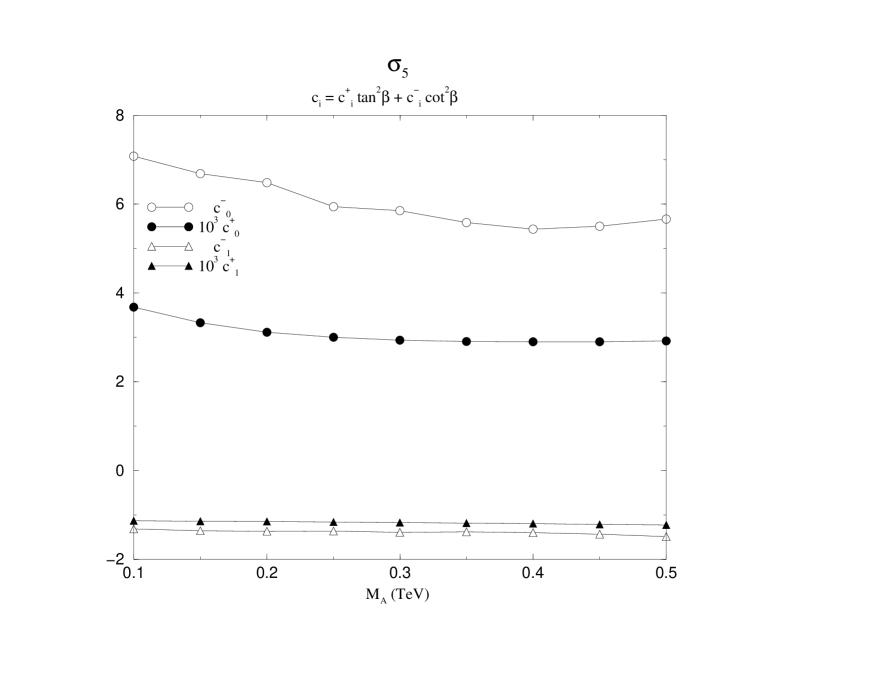
FIG. 13.: Dependence on $\tan\beta$ in the effective parametrization of the SUSY Higgses effects in $\sigma_{5}$. For each $M_{A}$, we determine the constants $c_{0,1}^{\pm}$ in $c_{i}=c_{i}^{+}\tan^{2}\beta+c_{i}^{-}\cot^{2}\beta$. This functional form turns out to be perfectly matched by the exact calculation. We interpret this fact as a dominance of the diagrams with exchange of charged SUSY Higgses that have rigorously this dependence on $\tan\beta$. Again, the coefficients of the logarithm, $c_{1}^{\pm}$ are roughly independent on $M_{A}$.

FIG. 14.: Effective parametrization of the SUSY Higgses effects in $\sigma_{5}$ in the energy range between 500 GeV and 1 TeV. This region is definitely non asymptotic and the constants $c_{0}$, $c_{1}$ afforded by the best fit procedure turn out to be strongly dependent on $M_{A}$ as discussed in the text.

REFERENCES

- [1] M. Beccaria, P. Ciafaloni, D. Comelli, F.M. Renard and C. Verzegnassi, Phys. Rev. D61,073005(2000).
- [2] M. Beccaria, P. Ciafaloni, D. Comelli, F.M. Renard and C. Verzegnassi, Phys.Rev. D61,011301(2000).
- [3] P. Ciafaloni, D. Comelli, Phys.Lett.B446,278(1999).
- [4] V. V. Sudakov, Sov. Phys. JETP 3, 65 (1956); Landau-Lifshits: Relativistic Quantum Field theory IV tome, ed. MIR.
- [5] M. Ciafaloni, P. Ciafaloni, D. Comelli, Phys.Rev.Lett.84,4810(2000); hep-ph/0004071; hep-ph/0007096.
- [6] H.P. Nilles, Phys.Rep. 110,1(1984); H.E. Haber and G.L. Kane, Phys. Rep. 117,75(1985); R. Barbieri, Riv.Nuov.Cim. 11,1(1988); R. Arnowitt, A, Chamseddine and P. Nath, ”Applied N=1 Supergravity (World Scientific, 1984); for a recent review see e.g. S.P. Martin, hep-ph/9709356v3(1999).
- [7] R. Barbieri, G.F. Giudice, Nucl.Phys.B306,63(1988).
- [8] Opportunities and Requirements for Experimentation at a Very High Energy Collider, SLAC-329(1928); Proc. Workshops on Japan Linear Collider, KEK Reports, 90-2, 91-10 and 92-16; P.M. Zerwas, DESY 93-112, Aug. 1993; Proc. of the Workshop on Collisions at 500 GeV: The Physics Potential, DESY 92-123A,B,(1992), C(1993), D(1994), E(1997) ed. P. Zerwas; E. Accomando et.al. Phys. Rep. (1998) 299.
- [9] ” The CLIC study of a multi-TeV linear collider”, CERN-PS-99-005-LP (1999).
- [10] F.M. Renard and C. Verzegnassi, Phys. Rev. D52, 1369 (1995), Phys. Rev. D53, 1290 (1996);M. Beccaria, F. Renard, S. Spagnolo, C. Verzegnassi, hep-ph/0002101; to appear in Phys.Rev.D.
- [11] G. Degrassi and A. Sirlin, Nucl. Phys. B 383, 73 (1992); Phys. Rev. D 46, 3104 (1992).
- [12] H. Georgi, H. Quinn and S. Weinberg, Phys.Rev.Lett.32,451(1974); S. Dimopoulos and H. Georgi, Nucl.Phys.B193,50(1981); S. Dimopoulos, S. Raby and F. Wilczek, Phys. Rev.D24,1681 (1981); L. Ibañez and GG. Ross, Phys.Lett.105B,439(1981).
- [13] M Boulware and D. Finnell, Phys.Rev.D44,2054(1991).
- [14] J. Rosiek, Phys.Rev.D41,3464(1990); erratum hep-ph/9511250.
- [15] F.M. Renard and C. Verzegnassi, Phys.Rev.D55,4370(1997).
- [16] A.Blondel, B.W.Lynn, F.M.Renard and C.Verzegnassi, Nucl.Phys.B304,438(1988).
- [17] S. Heinemeyer, W. Hollik, G. Weiglein, Comput.Phys.Commun.124,76(2000); hep-ph/9812320.
- [18] R. Barbieri, M. Beccaria, P. Ciafaloni, G. Curci, A. Vicere, Nucl.Phys. B409, 105 (1993); Phys.Lett. B288, 95 (1992), Erratum-ibid. B312, 511 (1993).
- [19] M. Beccaria, F.M. Renard and C. Verzegnassi, in preparation.