Anomalous magnetic moment of a bound electron

Abstract

We study binding corrections to the gyromagnetic factor $g_{\rm e}$ of an electron in hydrogen-like ions. We argue that the leading order binding effects in radiative corrections $\Delta g_{\rm rad}$ are universal to all orders in $\alpha/\pi$ and the complete result reads $\Delta g_{\rm rad}=(g_{\rm free}-2)\cdot[1+(Z\alpha)^{2}/6]+{\cal O}\left({\alpha\over\pi}\cdot(Z\alpha)^{4}\right)$. The theoretical uncertainty in the prediction for the experimentally interesting carbon ion is decreased by a factor of about 3.

The interaction of an electron with an external magnetic field $B$ is described by the potential

$$V=-\mbox{\boldmath$\mu$}\cdot\mbox{\boldmath$B$}.$$ (1)

The electron magnetic moment $\mu$ is

$$\mbox{\boldmath$\mu$}=g_{\rm e}\,{e\over 2m}\mbox{\boldmath$s$}.$$ (2)

where $m$ and $\mbox{\boldmath$s$}=\mbox{\boldmath$\sigma$}/2$ denote the mass and spin of the electron and $g_{\rm e}$ is the so-called gyromagnetic or Landé factor. We adopt the convention that $e=-|e|$.

For a free electron, $g_{\rm e}$ is known with very high precision. If an electron is bound in a ground state of a hydrogen-like ion, $g_{\rm e}$ becomes a function of the nuclear charge $Z$ and its measurements provide a sensitive test of the bound-state theory based on the Quantum Electrodynamics (QED). With a novel spectroscopic method precise experiments can be carried out with hydrogen-like ions in a wide range of nuclear charges $Z$ [1, 2, 3]. A unique feature of those measurements is that results obtained with different values of $Z$ may be used to rigorously test various bound-state effects [4].

To fully exploit these experimental results, the QED prediction for $g_{\rm e}\,(Z)$ must be known with comparable precision. At the present level of experimental uncertainty, accounting for the QED interactions (including leading effects of the nuclear recoil) is sufficient; other nuclear effects and weak interactions can be neglected. The theoretical prediction can be cast in the following form [5]

$$g_{\rm e}\,(Z)=g_{\rm D}+\Delta g_{\rm rec}+\Delta g_{\rm rad}.$$ (3)

The first term corresponds to the lowest order expansion in $\alpha/\pi$ and has been calculated to all orders in $Z\alpha$ [6],

$$g_{\rm D}={2\over 3}\left[1+2\sqrt{1-(Z\alpha)^{2}}\right].$$ (4)

$\Delta g_{\rm rec}$ denotes the recoil corrections [7], $\Delta g_{\rm rec}={\cal O}\left((Z\alpha)^{2}{m\over m_{N}}\right)$, where $m_{N}$ is the nucleus mass. Further references to the studies of those effects can be found in [5].

The main focus of the present paper are the radiative corrections. They can be presented as an expansion in two parameters, $Z\alpha$ and $\alpha/\pi$,

$${\Delta g_{\rm rad}\over 2}=C_{\rm e}^{(2)}(Z\alpha)\left({\alpha\over\pi}\right)+C_{\rm e}^{(4)}(Z\alpha)\left({\alpha\over\pi}\right)^{2}+\ldots$$ (5)

Powers of $\alpha/\pi$ correspond to electron–electron interactions, while $Z\alpha$ governs binding effects due to electron interactions with the nucleus. The binding effects are relatively more important, being enhanced by the nuclear charge and not suppressed by $1/\pi$, peculiar to the radiative corrections.

The first coefficient function in (5), $C_{\rm e}^{(2)}(Z\alpha)$, has been computed numerically to all orders in $Z\alpha$ [8, 9]. Its first two terms in the $Z\alpha$ expansion are also known analytically [10, 11]

$$C_{\rm e}^{(2)}(Z\alpha)={1\over 2}\left[1+{1\over 6}(Z\alpha)^{2}+{\cal O}\left((Z\alpha)^{4}\right)\right].$$ (6)

The main theoretical uncertainty for $g_{\rm e}$ in light ions is, at present, connected with the unknown coefficient $C^{\prime}$ in the next coefficient function,

$$C_{\rm e}^{(4)}(Z\alpha) = C_{\rm e}^{(4)}(0)\left[1+C^{\prime}\cdot(Z\alpha)^{2}+{\cal O}\left((Z\alpha)^{4}\right)\right],$$ (7)

$$C_{\rm e}^{(4)}(0) = -0.328\,478\,444\,00\ldots\qquad\cite[cite]{[\@@bibref{Number}{som57,pet57a,Mohr99}{}{}]}.$$ (8)

At present, the most accurate experimental value of the bound electron gyromagnetic factor has been obtained [14, 15] with a hydrogen-like carbon ion ¹²C⁵⁺ ($Z=6$),

$$g_{\rm e}(Z=6;{\rm exp})=2.001\,041\,596(5).$$ (9)

The theoretical prediction is [16]

$$g_{\rm e}(Z=6;{\rm theory})=2.001\,041\,591(7)$$ (10)

where 70% of the error is caused by the unknown coefficient $C^{\prime}$ of the $\left({\alpha\over\pi}\right)^{2}(Z\alpha)^{2}$ effects in (8) (for carbon, higher powers of $Z\alpha$ are assumed to be negligible).

The purpose of this paper is to demonstrate that $C^{\prime}={1/6}$, in analogy to the corresponding coefficient in the lower order in $\alpha/\pi$. In fact, we will see that the coefficient of $(Z\alpha)^{2}$ is the same in all coefficient functions $C^{(2n)}_{e}(Z\alpha)$, so that the theoretical prediction for $\Delta g_{\rm rad}$ accurate up to $(Z\alpha)^{2}$ and exact in $\alpha/\pi$ reads:

$$\Delta g_{\rm rad}=(g_{\rm free}-2)\cdot\left[1+{(Z\alpha)^{2}\over 6}\right],$$ (11)

where $g_{\rm free}$ is the gyromagnetic factor of a free electron, presently known to ${\cal O}\left((\alpha/\pi)^{4}\right)$ [17]. With this result, the theoretical uncertainty in (10) is reduced from $7\cdot 10^{-9}$ to about $2\cdot 10^{-9}$.

To prove Eq. (11), we begin with a derivation of the ${\cal O}\left((Z\alpha)^{2}\right)$ term in the Breit correction (4), working in full QED. We will try to interpret the result in the language of effective potentials whose average values give the required correction. In the next step we will construct from those operators an effective Hamiltonian with which we will be able to evaluate $(Z\alpha)^{2}$ corrections to higher orders in $\alpha/\pi$.

There are two contributions which have to be considered, shown in Fig. 1. The velocity of the electron in the ion is of the order of $Z\alpha$; in order to compute corrections $(Z\alpha)^{2}$, it is sufficient to expand the matrix elements to second order in electron momentum, relative to the leading term.

The diagram 1(a) describes the scattering of an electron on the magnetic field $B$. Expanding this matrix element with respect to electron’s velocity we arrive at the following effective potential:

$$\Delta V_{a} =-\frac{e}{2m}\left\{\mbox{\boldmath$\sigma$}\cdot\mbox{\boldmath$B$}\left(1-\frac{\mbox{${\mbox{\boldmath$p$}}$}^{2}}{2m^{2}}\right)\right.$$ (13)

$$\left.+\frac{i}{4m}\left[H+\frac{Z\alpha}{r},\mbox{\boldmath$\sigma$}\cdot\left(\mbox{${\mbox{\boldmath$A$}}$}\times\mbox{${\mbox{\boldmath$p$}}$}-\mbox{${\mbox{\boldmath$p$}}$}\times\mbox{${\mbox{\boldmath$A$}}$}\right)\right]\right\},$$

where $H=\mbox{${\mbox{\boldmath$p$}}$}^{2}/2m-Z\alpha/r$ is the non-relativistic Hamiltonian. Since $\langle\Psi|[H,U]|\Psi\rangle=0$ for any operator $U$, we find the following expression for $\Delta V_{a}$

$$\Delta V_{a} =-\frac{e}{2m}\left\{\mbox{\boldmath$\sigma$}\cdot\mbox{\boldmath$B$}\left(1-\frac{\mbox{${\mbox{\boldmath$p$}}$}^{2}}{2m^{2}}\right)\right.$$ (15)

$$\left.-\frac{e}{4m}\mbox{\boldmath$\sigma$}\cdot\left(\mbox{${\mbox{\boldmath$A$}}$}\times\mbox{\boldmath$E$}-\mbox{\boldmath$E$}\times\mbox{${\mbox{\boldmath$A$}}$}\right)\right\}.$$

The Z-diagram in Fig. 1(b) describes a transition of the electron into the negative energy sea after interacting with either magnetic or electric field. Since the energy of the intermediate state is of the order of the electron mass, this is a short distance process and it can be described by a local operator,

$$\Delta V_{b}=-\frac{e^{2}}{4m^{2}}\mbox{\boldmath$\sigma$}\cdot\left(\mbox{${\mbox{\boldmath$A$}}$}\times\mbox{\boldmath$E$}-\mbox{\boldmath$E$}\times\mbox{${\mbox{\boldmath$A$}}$}\right).$$ (16)

The sum of contributions (15) and (16) reads

$$\Delta V =-\frac{e}{2m}\left\{\mbox{\boldmath$\sigma$}\cdot\mbox{\boldmath$B$}\left(1-\frac{\mbox{${\mbox{\boldmath$p$}}$}^{2}}{2m^{2}}\right)\right.$$ (18)

$$\left.+\frac{e}{4m}\mbox{\boldmath$\sigma$}\cdot\left(\mbox{${\mbox{\boldmath$A$}}$}\times\mbox{\boldmath$E$}-\mbox{\boldmath$E$}\times\mbox{${\mbox{\boldmath$A$}}$}\right)\right\},$$

and, after being averaged over the $1S$ state, gives the leading binding correction to the $g_{\rm e}$-factor:

$$g_{\rm D}\simeq 2-\frac{2(Z\alpha)^{2}}{3},$$ (19)

which agrees with first two terms of expansion of Eq. (4).

We remark that there could be another source of $(Z\alpha)^{2}$ corrections induced by Breit potential $V_{\rm Breit}$,

$$\langle 1S|\mbox{\boldmath$\sigma$}\cdot\mbox{\boldmath$B$}\sum\limits_{n\neq 1}\frac{|n\rangle\langle n|}{E-E_{n}}V_{\rm Breit}|1S\rangle.$$

However, this expression vanishes for the constant magnetic field $B$, and therefore the result in (19) is complete.

Although Eq. (18) leads to a correct result, its second term depends on the electromagnetic potential $A$ and therefore is not gauge invariant. How is the gauge invariance restored? The answer is that there should be an additional $A$-independent contribution to the potential, so that the second term in Eq. (18) is a part of an explicitly gauge invariant expression

$$\frac{e}{8m^{2}}\mbox{\boldmath$\sigma$}\cdot\left(\mbox{${\mbox{\boldmath$P$}}$}\times{\mbox{\boldmath$E$}}-\mbox{\boldmath$E$}\times\mbox{${\mbox{\boldmath$P$}}$}\right),$$ (20)

where $\mbox{${\mbox{\boldmath$P$}}$}=\mbox{${\mbox{\boldmath$p$}}$}-e\mbox{${\mbox{\boldmath$A$}}$}$ is the canonical momentum of the Coulomb Hamiltonian. Although this operator depends on both $E$ and $A$, its coefficient can be determined more easily by switching off the magnetic field and considering the scattering of an electron on an electric field alone.

The above considerations suggest the form of the general effective Hamiltonian describing the interaction of an electron with a magnetic field $B$, in the presence of an electric field $E$,

$$\Delta H = -c_{0}{e\over 2m}\mbox{\boldmath$\sigma$}\cdot\mbox{\boldmath$B$}+c_{1}{e\over 8m^{2}}{\mbox{\boldmath$\sigma$}\cdot\left(\mbox{\boldmath$P$}\times\mbox{\boldmath$E$}-\mbox{\boldmath$E$}\times\mbox{\boldmath$P$}\right)}$$ (22)

$$+c_{2}\frac{e}{4m^{3}}\,\mbox{\boldmath$p$}^{2}\;\mbox{\boldmath$\sigma$}\cdot\mbox{\boldmath$B$}+c_{3}\frac{e}{4m^{3}}\,\mbox{\boldmath$p$}\cdot\mbox{\boldmath$B$}\;\mbox{\boldmath$\sigma$}\cdot\mbox{\boldmath$p$}.$$

The coefficients $c_{i}$ can be found by the standard procedure of matching the amplitudes obtained within the effective theory with those in the full QED [18]. To this end, we consider the on-shell elastic scattering of an electron on the electric field (for $c_{1}$) or on the magnetic field (for $c_{0,2,3}$). The interaction of an electron with the electromagnetic field is described by two form factors (in the absence of parity violation),

$$\langle e(p^{\prime})|J^{\rm em}_{\mu}|e(p)\rangle$$ (24)

$$=e\,\bar{u}_{e}(p^{\prime})\left(F_{D}(q^{2})\gamma^{\mu}+{i\over 2m}F_{P}(q^{2})\,\sigma^{\mu\nu}q_{\nu}\right)u_{e}(p).$$

Here $q=p^{\prime}-p$. For the determination of $c_{i}$ we can treat the external fields as constant, and need the form factors only at $q^{2}=0$. In this case the Dirac form factor is $F_{D}(0)=1$ and the Pauli form factor gives the anomalous magnetic moment $F_{P}(0)=\alpha/2\pi+C^{(4)}_{e}(0)\,(\alpha/\pi)^{2}+\ldots$.

The form of interaction (24) determines the scattering amplitudes in external magnetic and electric fields, and we easily find the coefficients of the relevant operators in (22),

$$c_{0} = F_{D}+F_{P},\qquad c_{1}=F_{D}+2F_{P},$$ (25)

$$c_{2} = F_{D},\qquad c_{3}=F_{P}.$$ (26)

To find the interaction energy of a bound electron in an external magnetic field, we compute the expectation value of the Hamiltonian (22) in the $1S$ state and find

$$V = -{e\over 2m}(F_{D}+F_{P})\mbox{\boldmath$\sigma$}\cdot\mbox{\boldmath$B$}$$ (28)

$$-{e\over 2m}(Z\alpha)^{2}\left({F_{P}-2F_{D}\over 6}\right)\mbox{\boldmath$\sigma$}\cdot\mbox{\boldmath$B$}+{\cal O}\left((Z\alpha)^{4}\right).$$

Comparing this result with (1) and (2) we find (neglecting nuclear recoil and effects of ${\cal O}\left((Z\alpha)^{4}\right)$)

$${g_{\rm e}(Z)\over 2}=F_{D}+F_{P}+(Z\alpha)^{2}{F_{P}-2F_{D}\over 6}.$$ (29)

This result is valid to all orders in the “radiative” expansion parameter $\alpha/\pi$. We can re-write it as

$${g_{\rm e}(Z)\over 2} = \left(1-{(Z\alpha)^{2}\over 3}\right)+F_{P}\left(1+{(Z\alpha)^{2}\over 6}\right)$$ (30)

$$= {g_{\rm D}\over 2}+\left[{\alpha\over 2\pi}+C_{\rm e}^{(4)}(0)\,\left({\alpha\over\pi}\right)^{2}+\ldots\right]$$ (32)

$$\times\left(1+{(Z\alpha)^{2}\over 6}\right)+{\cal O}\left((Z\alpha)^{4}\right).$$

Comparing this with eqs. (4, 6), we see that we have correctly reproduced the known 0- and 1-loop results. We have also found, that the bound-state correction factor $C^{\prime}={1/6}$ is universal in all orders in $\alpha/\pi$.

Summary

We have demonstrated a relation between the gyromagnetic factors of free and bound electrons, valid to the lowest order in $(Z\alpha)^{2}$ and to all orders in $\alpha/\pi$. The main reason for this somewhat unexpected relation is that only low-dimensional effective operators contribute to order $(Z\alpha)^{2}$.

We do not anticipate a similar relation involving only known form factors $F_{D}$ and $F_{P}$ to hold for the higher order binding effects. For example, in ${\cal O}\left((Z\alpha)^{4}\right)$, the operator $\mbox{\boldmath$\sigma$}\cdot\mbox{\boldmath$B$}\,(\mbox{\boldmath$E$}\cdot\mbox{\boldmath$p$}+\mbox{\boldmath$p$}\cdot\mbox{\boldmath$E$})$ might contribute. In general, the coefficients of such operators in the effective Hamiltonian are new functions of $\alpha/\pi$, independent of $F_{D,P}$.

In the previous theoretical prediction for the bound electron $g_{\rm e}$ [16], the main source of uncertainty was the unknown two-loop binding effect, which has been estimated as $3\alpha/\pi$ times the one-loop binding effect. For $Z=6$ it is $3(\alpha/\pi)^{2}\cdot(Z\alpha)^{2}/6\simeq 5\cdot 10^{-9}$. Together with the error in the nuclear recoil, the total theoretical uncertainty was estimated as $7\cdot 10^{-9}$. The result of the present paper, which gives the explicit two-loop binding effect, shifts the central value of the theoretical prediction, eq. (10), by $-1.13\cdot 10^{-9}$, and reduces its uncertainty by a factor of about 3. The remaining uncertainty is dominated by the errors of the recoil correction $\Delta g_{\rm rec}$ and of the numerical evaluation of the binding effects in the order ${\alpha/\pi}$ (see [16] for a detailed discussion). With this reduction in the theoretical uncertainty, a very precise value of the electron mass can be extracted from bound electron $g$-factor experiments [19].

Finally, let us note that a confrontation of the theoretical prediction (10) with the experimental results (9) for $g_{\rm e}$ tests the bound-state QED at the level of 1%. For comparison, measurements of the positronium hyperfine splitting test the bound-state QED effects at the level of 0.3% [20, 21, 22]. If the experimental uncertainty in the bound electron $g$-factor can be further reduced, its measurements, combined with an independent electron mass determination, will rank among the most stringent tests of the relativistic bound-state theory.

Note added. After completing this work, we learned about Ref. [23], where ${\cal O}\left((Z\alpha)^{2}\right)$ corrections were also considered. Although our approach differs substantially from that of Ref. [23], the final results agree. Our paper should, therefore, be viewed as an alternative way of deriving the binding ${\cal O}\left((Z\alpha)^{2}\right)$ corrections to the gyromagnetic factor of the electron. We believe, however, that the results of Ref. [23] have not become well known; for this reason our alternative derivation and the emphasis on phenomenological consequences seems to be timely.

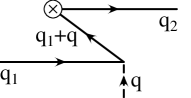
      (a) (b)

FIG. 1.: Tree-level contributions to the factor $g$ of a bound electron. The cross denotes the magnetic field insertion, and the dashed line is the interaction with the Coulomb field. The diagram (b) has a counterpart with the electric and magnetic fields interchanged.

REFERENCES

- [1] N. Hermanspahn et al., Acta Phys. Pol. B27, 357 (1996).
- [2] W. Quint, Phys. Scr. T59, 203 (1995).
- [3] G. Werth, Phys. Scr. T59, 206 (1995).
- [4] S. G. Karshenboim, Phys. Lett. A266, 380 (2000).
- [5] P. J. Mohr and B. N. Taylor, Rev. Mod. Phys. 72, 351 (2000).
- [6] G. Breit, Nature 122, 649 (1928).
- [7] H. Grotch, Phys. Rev. A2, 1605 (1970).
- [8] A. Blundell, K. T. Cheng, and J. Sapirstein, Phys. Rev. 55, 1857 (1997).
- [9] H. Persson, S. Salomonson, P. Sunnergren, and I. Lindgren, Phys. Rev. 56, R2499 (1997).
- [10] J. Schwinger, Phys. Rev. 73, 416 (1948).
- [11] H. Grotch, Phys. Rev. Lett. 24, 39 (1970).
- [12] C. M. Sommerfield, Phys. Rev. 107, 328 (1957).
- [13] A. Petermann, Nucl. Phys. 3, 689 (1957).
- [14] N. Hermanspahn et al., Phys. Rev. Lett. 84, 427 (2000).
- [15] H. Häffner et al., The -Factor of Hydrogenic Ions: A Test of QED, 2000, contribution to the Conference Hydrogen Atom II, Castiglione della Pescaia, Italy, June 2000.
- [16] T. Beier et al. (unpublished).
- [17] V. W. Hughes and T. Kinoshita, Rev. Mod. Phys. 71, S133 (1999).
- [18] W. E. Caswell and G. P. Lepage, Phys. Lett. B167, 437 (1986).
- [19] G. Werth, private communication.
- [20] K. Pachucki, Phys. Rev. A56, 297 (1997).
- [21] K. Pachucki and S. G. Karshenboim, Phys. Rev. Lett. 80, 2101 (1998).
- [22] A. Czarnecki, K. Melnikov, and A. Yelkhovsky, Phys. Rev. Lett. 82, 311 (1999).
- [23] M. I. Eides and H. Grotch, Ann. Phys. 260, 191 (1997).
(a)
(b)
(a)
(b)