Predicting $D\to\sigma\pi$

Abstract

We examine the $D\to\sigma\pi$ amplitude through a constituent quark-meson model, incorporating heavy quark and chiral symmetries, finding a good agreement with the recent E791 data analysis of $D\to 3\pi$ via $\sigma$.
Pacs numbers: 13.25.Ft, 12.39.Hg, 14.40.Cs
BARI-TH/00-393
UGVA-DPT/2000-07-1086

The light $\sigma$ resonance has accumulated considerable theoretical and experimental interest after it was reintroduced as a very broad resonance into the 1996 edition of the Reviews of Particle Physics [1]. Recently a conference[2] (at the Yukawa Institute for Theoretical Physics) was entirely devoted to this controversial resonance. The broad $\sigma$ has been difficult to disentangle from the available data, because the analyses require sophisticated theoretical models, which apart from unitarity, analyticity and coupled channels, also involve constrains from chiral and flavour symmetries.

A direct experimental evidence seems to emerge from the $D^{+}\to\sigma\pi^{+}\to 3\pi$ decay channel observed by the E791 collaboration [3], where the $\sigma$ is seen as a clear dominant peak covering $46\%$ of the $3\pi$ Dalitz plot. The reason why it is so prominent in this reaction, is that the background is small since S-waves dominate all subchannels, and the Adler zero (which complicate the analysis in $\pi\pi\to\pi\pi$ since there it suppresses the low energy tail of the $\sigma$ signal) is absent in the production of $\sigma$ in $D\to\sigma\pi$. In this letter we shall adopt a Constituent-Quark-Meson model, the CQM model [4], to calculate the amplitude for the process $D\to\sigma\pi$ and compare this prediction with E791 data analysis. CQM is an effective model that enables to calculate heavy meson decay amplitudes through diagrams where heavy mesons are attached at the ends of loops containing heavy and light quark internal lines. Essentially it is based on a Nambu-Jona-Lasinio effective Lagrangian whose bosonization is responsible for effective vertices (heavy meson)-(heavy quark)-(light quark). The model is relativistic and incorporates the heavy quark symmetries and the chiral $SU_{2}$ symmetry for the light quark sector of the Lagrangian.

In the following we will make use of the heavy meson field notation with $H$ and $S$ representing respectively the heavy meson degenerate $J^{P}$ doublets $(0^{-},1^{-})$ and $(0^{+},1^{+})$ predicted by Heavy-Quark-Effective-Theory (HQET) [5]. For our purposes $H$ and $S$ will represent the charmed mesons $D$ and $D(1^{+})$. The physical characteristics of the latter have been experimentally observed by the CLEO collaboration [6].

We will focus on the polar and direct contributions (shown in Figs. 1,2 and 3 respectively) to the $D\to\sigma$ semileptonic amplitude $\langle\sigma|A^{\mu}|D\rangle$. These contributions have been extensively discussed also in the analysis of the $B\to\pi$ semileptonic decay [7]. We first consider the polar contribution (Figs. 1,2). This reduces to a loop diagram in the CQM approach. According to the rules described in [4], the loop shown in Fig. 2, describing the amplitude $\langle S(1^{+})\sigma|H\rangle$, is computed through the following integral:

$$(-1)i^{3}(-i)^{3}\sqrt{Z_{H}Z_{S}m_{H}m_{S}}\frac{N_{c}}{16\pi^{4}}\int^{\rm reg}d^{4}l\frac{{\rm Tr}\left[(\gamma\cdot l+m)g_{\sigma qq}(\gamma\cdot(l+q_{\sigma})+m)\epsilon^{\mu}\gamma_{\mu}\gamma_{5}\frac{1+\gamma\cdot v}{2}(-\gamma_{5})\right]}{(l^{2}-m^{2})((l+q_{\sigma})^{2}-m^{2})(v\cdot l+\Delta_{H})},$$ (1)

where $\epsilon^{\mu}$ is the polarization of the $S(1^{+})$ state, $q^{\mu}_{\sigma}=m_{\sigma}v^{\prime\mu}$, $\Delta_{H}=M_{H}-m_{Q}$, being $M_{H}$ the mass of the incoming heavy meson (see Fig. 1,2), $v$ its four-velocity and $m_{Q}$ the mass of the constituent heavy quark there contained ($m_{Q}=m_{c}$ in our case). As for the constants, $(-1)$ comes from the fermion loop, $i^{3}$ from the three propagators and $(-i)^{3}$ from the three vertices (the vertices $HQq$ and $SQq$ are discussed in [4], while the vertex $qq\sigma$, brings the third factor of $(-i)$ [8])

After a continuation of the light propagator in the Euclidean domain, the regularization prescription adopted for the computation of the loop integral is the following:

$$\int d^{4}l_{E}\frac{1}{l^{2}_{E}+m^{2}}\to\int d^{4}l_{E}\int_{1/\Lambda^{2}}^{1/\mu^{2}}dse^{-s(l_{E}^{2}+m^{2})}.$$ (2)

The infrared and ultraviolet cutoffs $\mu$ and $\Lambda$ are respectively $\mu=300$ MeV and $\Lambda=1.25$ GeV. The mass $m$ is the constituent mass of the light quark as obtained by a NJL gap-equation; its value is $m=300$ MeV. A discussion about the choice of these values can be found in [4]. What should be remarked here is that once fixed $\Lambda$ and $\mu$, the light constituent mass $m$ is determined. Varying the cutoffs requires also a recomputation of $m$. For $m$ values close to $300$ MeV, infrared and ultraviolet cutoffs can range only in a narrow spread of values.

The renormalization constants appearing in (1) are:

$$Z_{H}^{-1} = (\Delta_{H}+m){\frac{\partial I_{3}(\Delta_{H})}{\partial\Delta_{H}}}+I_{3}(\Delta_{H})$$ (3)

$$Z_{S}^{-1} = (\Delta_{S}-m){\frac{\partial I_{3}(\Delta_{S})}{\partial\Delta_{S}}}+I_{3}(\Delta_{S}),$$ (4)

where:

$$I_{3}(\Delta) = -\frac{iN_{c}}{16\pi^{4}}\int^{\mathrm{reg}}\frac{d^{4}l}{(l^{2}-m^{2})(v\cdot l+\Delta+i\epsilon)}$$ (5)

$$= {N_{c}\over{16\,{{\pi}^{{3/2}}}}}\int_{1/{{\Lambda}^{2}}}^{1/{{\mu}^{2}}}{ds\over{s^{3/2}}}\;e^{-s({m^{2}}-{{\Delta}^{2}})}\;\left(1+{\mathrm{erf}}(\Delta\sqrt{s})\right),$$ (6)

and $\Delta_{S}$ is defined in the same way as $\Delta_{H}$, i.e., $\Delta_{S}=M_{S}-m_{Q}$. $\Delta_{H}$ is the main free parameter of the model. For it we choose three reasonable values $\Delta_{H}=0.3,0.4,0.5$ GeV. All other quantities, including $\Delta_{S}$, vary accordingly. The number of colours is $N_{c}=3$. The coupling $g_{\sigma qq}$ of the $\sigma$ meson field to the light quark fields emerges through the bosonization of a NJL Lagrangian density leading to a linear $\sigma-$model of composite fields, as discussed in [8]:

$$g_{\sigma qq}=\frac{1}{2\sqrt{I_{2}}},$$ (7)

where:

$$I_{2}=-\frac{iN_{c}}{16\pi^{4}}\int^{\mathrm{reg}}\frac{d^{4}l}{(l^{2}-m^{2})^{2}}=\frac{N_{c}}{16\pi^{2}}\Gamma\left(0,\frac{m^{2}}{\Lambda^{2}},\frac{m^{2}}{\mu^{2}}\right).$$ (8)

Numerically:

$$g_{\sigma qq}=2.49.$$ (9)

Defining the coupling:

$$\langle D(1^{+})(p^{\prime})\sigma(q_{\sigma})|D(p)\rangle=-iG_{DD(1^{+})\sigma}\epsilon\cdot q_{\sigma},$$ (10)

the computation of the loop integral (1) gives, comparing (1) and (10):

$$G_{HS\sigma}=2g_{\sigma qq}C\sqrt{Z_{H}Z_{S}m_{H}m_{S}},$$ (11)

where $C$ is:

$$C = \frac{1}{2m_{\sigma}}\left(I_{3}\left(\frac{m_{\sigma}}{2}\right)-I_{3}\left(-\frac{m_{\sigma}}{2}\right)\right)+(m+\Delta_{H})Z-\frac{(\Delta_{S}-\Delta_{H})-2m}{m_{\sigma}}\Omega_{2},$$ (12)

and:

$$Z = \frac{iN_{c}}{16\pi^{4}}\int^{\mathrm{reg}}\frac{d^{4}l}{(l^{2}-m^{2})[(l+q)^{2}-m^{2}](v\cdot l+\Delta_{1}+i\epsilon)}$$ (13)

$$= \frac{I_{5}(\Delta_{1},x/2,\omega)-I_{5}(\Delta_{2},-x/2,\omega)}{2x}.$$ (14)

In the case at hand, $\Delta_{1}=\Delta_{H}$, $\Delta_{2}=\Delta_{S}$, $x=m_{\sigma}$ and:

$$\omega=v\cdot v^{\prime}=\frac{v\cdot q_{\sigma}}{m_{\sigma}}=\frac{v\cdot k-v\cdot k^{\prime}}{m_{\sigma}}=\frac{\Delta_{H}-\Delta_{S}}{m_{\sigma}},$$ (15)

where $k$ and $k^{\prime}$ are the residual momenta related to the $H$ and $S$ fields as in Fig 2. The $I_{5}$ integral is computed defining:

$$\eta(x,\Delta_{1},\Delta_{2},\omega)={{{\Delta_{1}}\,\left(1-x\right)+{\Delta_{2}}\,x}\over{{\sqrt{1+2\,\left(\omega-1\right)\,x+2\,\left(1-\omega\right)\,{x^{2}}}}}}.$$ (16)

The explicit expression is:

$$I_{5}(\Delta_{1},\Delta_{2},\omega) = \frac{iN_{c}}{16\pi^{4}}\int^{\mathrm{reg}}\frac{d^{4}l}{(l^{2}-m^{2})(v\cdot l+\Delta_{1}+i\epsilon)(v^{\prime}\cdot l+\Delta_{2}+i\epsilon)}$$ (17)

$$= \int_{0}^{1}dx\frac{1}{1+2x^{2}(1-\omega)+2x(\omega-1)}\times$$ (20)

$$\Big{[}\frac{6}{16\pi^{3/2}}\int_{1/\Lambda^{2}}^{1/\mu^{2}}ds~{}\eta\;e^{-s(m^{2}-\eta^{2})}\;s^{-1/2}\;(1+{\mathrm{erf}}(\eta\sqrt{s}))+$$

$$\frac{6}{16\pi^{2}}\int_{1/\Lambda^{2}}^{1/\mu^{2}}ds\;e^{-s(m^{2}-2\eta^{2})}\;s^{-1}\Big{]}.$$

Moreover:

$$\Omega_{2}=\frac{-I_{3}(\Delta_{1})+I_{3}(\Delta_{2})-\omega[I_{3}(-x/2)-I_{3}(x/2)]}{2x(1-\omega^{2})}-\frac{[x/2-\Delta_{1}\omega]Z}{1-\omega^{2}},$$ (21)

where again $\Delta_{1}=\Delta_{H}$, $\Delta_{2}=\Delta_{S}$ and $x=m_{\sigma}$.

Let’s write the weak current matrix element for the semileptonic transition amplitude $D\to\sigma$:

$$\langle\sigma(q_{\sigma})|A^{\mu}(q)|D(p)\rangle = \left[(p+q_{\sigma})^{\mu}+\frac{m_{\sigma}^{2}-m_{D}^{2}}{q^{2}}q^{\mu}\right]\;F_{1}(q^{2})$$ (22)

$$- \left[\frac{m_{\sigma}^{2}-m_{D}^{2}}{q^{2}}q^{\mu}\right]\;F_{0}(q^{2}),$$ (23)

with $F_{1}(0)=F_{0}(0)$. Defining:

$$\langle{\rm VAC}|A^{\mu}|D(1^{+})\rangle=\hat{F}^{+}\sqrt{m_{D(1^{+})}}\epsilon^{\mu},$$ (24)

we have:

$$F_{1}(q^{2})=\frac{1}{2}\times\frac{\sqrt{m_{D(1^{+})}}\hat{F}^{+}G_{DD(1^{+})\sigma}}{m_{D(1^{+})}^{2}-q^{2}}.$$ (25)

This is equivalent to assuming a polar model for the form factor $F_{1}(q^{2})$ with $D(1^{+})$ taken as the intermediate virtual state (see Figs. 1,2). The polar form factors are obviously more reliable near the pole, where $q^{2}\simeq m_{S}^{2}$, than in the small $q^{2}$ range. Anyway we assume the polar behavior valid for the whole $q^{2}$ range. For our purposes the $\sigma$ meson is a $J^{PC}=0^{++}$ isoscalar with a quark content $(\bar{u}u+\bar{d}d)$.

Using the values $m_{\sigma}=478$ MeV [3], $m_{S}=2.461$ GeV [6], $m_{H}=1.869$ GeV [1] and $\hat{F}^{+}$ given by the CQM model as a function of $\Delta_{H}$ [4] we have, varying $\Delta_{H}$ (and consequently $\Delta_{S}$, see [4]) in the range of values $0.3,0.4,0.5$ GeV:

$$F_{1}^{\rm pol}(0)=0.30\pm 0.04.$$ (26)

The same calculation for $F_{0}(q^{2})$ implies to consider the $D$ meson in the dispersion relation. Assuming that we can extrapolate the polar behaviour to $q^{2}=0$ leads to:

$$F_{0}^{\rm pol}(0)=\frac{\hat{F}G_{DD\sigma}}{2m_{D}^{5/2}},$$ (27)

where $\hat{F}$ is defined by:

$$\langle{\rm VAC}|A^{\mu}|D(p)\rangle=ip^{\mu}\frac{\hat{F}}{\sqrt{m_{D}}},$$ (28)

and is computed in CQM [4]; $G_{DD\sigma}$ is given by:

$$G_{DD\sigma}=2g_{\sigma qq}Z_{H}m_{H}(2m\Omega_{1}-m^{2}Z),$$ (29)

with:

$$\Omega_{1}=\frac{I_{3}(-x/2)-I_{3}(x/2)+\omega[I_{3}(\Delta_{1})-I_{3}(\Delta_{2})]}{2x(1-\omega^{2})}-\frac{[\Delta_{1}-\omega x/2]Z}{1-\omega^{2}},$$ (30)

where $\Delta_{1}=\Delta_{H}=\Delta_{2}$ and $\omega=0$. The numerical result is:

$$F_{0}^{\rm pol}(0)=0.22_{-0.01}^{+0.07}.$$ (31)

Let us now consider the direct contribution of Fig. 3, obtaining:

$$F_{1}^{\rm dir}(q^{2})=2\sqrt{Z_{H}m_{H}}g_{\sigma qq}\left(\frac{c\Omega_{1}}{2m_{H}}+\frac{c\Omega_{2}}{2m_{\sigma}}-\frac{a}{2m_{H}}-\frac{b}{2}\right),$$ (32)

where:

$$a = -I_{3}(\Delta)+2m^{2}Z+m_{\sigma}(\omega\Omega_{1}+\Omega_{2})$$ (33)

$$b = \frac{1}{2m_{\sigma}}\left[I_{3}\left(-\frac{m_{\sigma}}{2}\right)-I_{3}\left(\frac{m_{\sigma}}{2}\right)\right]-(\Delta_{H}+m)Z$$ (34)

$$c = (m_{\sigma}\omega+2m),$$ (35)

and we notice that $\omega=\frac{m_{D}^{2}+m_{\sigma}^{2}-q^{2}}{2m_{D}m_{\sigma}}$, $\Delta=\Delta_{H}-m_{\sigma}\omega$, $\Delta_{1}=\Delta_{H}$, $\Delta_{2}=\Delta$, $x=m_{\sigma}$. Numerically:

$$F_{1}^{\rm dir}(q^{2}=0)=0.30\pm 0.02.$$ (36)

The analogous result for $F_{0}^{\rm dir}(q^{2})$ is:

$$F_{0}^{\rm dir}(q^{2})=2\sqrt{Z_{H}m_{H}}g_{\sigma qq}\left[\left(\frac{c\Omega_{1}-a}{2m_{H}}\right)\left(1+\frac{q^{2}}{m_{D}^{2}-m_{\sigma}^{2}}\right)+\left(\frac{c\Omega_{2}}{2m_{\sigma}}-\frac{b}{2}\right)\left(1-\frac{q^{2}}{m_{D}^{2}-m_{\sigma}^{2}}\right)\right]$$ (37)

with $F_{0}^{\rm dir}(q^{2}=0)=0.30\pm 0.02$. We conclude that the CQM-model analysis gives:

$$F_{0}^{\rm pol}(0)+F_{0}^{\rm dir}(0)=0.52^{+0.09}_{-0.03},$$ (38)

We have not included in this analysis the uncertainty arising from the extrapolation to $q^{2}=m_{\pi}^{2}\simeq 0$ of the result obtained by the dispersion relation, strictly valid only for $q^{2}\simeq m_{D}^{2}$. We can estimate it by considering that $F_{1}(0)=F_{1}^{\rm pol}(0)+F_{0}^{\rm dir}(0)$ should be equal to $F_{0}(0)$. Our result for $F_{1}(0)$ is:

$$F_{1}(0)=0.60\pm 0.06,$$ (39)

which agrees within errors with the number obtained in (38). Our estimate is therefore:

$$F_{0}(m_{\pi}^{2})\simeq F_{0}(0)=0.57\pm 0.09.$$ (40)

This result has to be compared with that obtained directly from preliminary E791 data [9]:

$$F_{0}(m_{\pi}^{2})=0.79\pm 0.15,$$ (41)

by means of the following expression for the $D\to\sigma\pi$ amplitude:

$$\langle\sigma\pi^{+}|H_{\rm eff}|D^{+}\rangle=\frac{G_{F}}{\sqrt{2}}V^{*}_{cd}V_{ud}a_{1}F_{0}(m_{\pi}^{2})(m_{D}^{2}-m_{\sigma}^{2})f_{\pi},$$ (42)

where $H_{\rm eff}$ is the effective Hamiltonian of Bauer, Stech and Wirbel [10], with $a_{1}=1.10\pm 0.05$ fitted for $D$ decays while the value for the amplitude $\langle\sigma\pi^{+}|H_{\rm eff}|D^{+}\rangle$ is computed considering the experimental evidence for $\Gamma(D^{+}\to\sigma\pi^{+}\to\pi^{+}\pi^{-}\pi^{+})=0.44\times\Gamma(D^{+}\to\pi^{+}\pi^{-}\pi^{+})$ and taking the strong coupling constant $g_{\sigma\pi\pi}$ derived from the preliminary E791 fit for the sigma width $\Gamma_{\sigma}=338\pm 48$ MeV [9].

We are aware of the theoretical uncertainties of the present calculation; in particular, $1/m_{c}$ corrections, that have been neglected in the quark loop calculation and in the evaluation of $\hat{F}^{+}$, may alter our result (40). To estimate these uncertainties we note that CQM can be applied to the evaluation of the coupling $F_{1}^{(D\pi)}(0)$ for which experimental data are also available. We observe that in the case of the $D\to\pi$ semileptonic process, the polar form factor $F_{1}^{(D\pi)}(0)$ can be obtained from $F_{1}^{(B\pi)}(0)$, computed in [7] by CQM, simply using the following scaling form [11]:

$$F_{1}^{(D\pi)}(0)=\sqrt{\frac{m_{B}}{m_{D}}}F_{1}^{(B\pi)}(0)=0.87\pm 0.02,$$ (43)

(neglecting small QCD corrections) since the computation of $F_{1}^{(B\pi)}(0)$ is more stable against $1/m_{Q}$ corrections. This must be compared with the $F^{(D\pi)}_{1}(0)=0.78\pm 0.06$, deducible from the PDG [1], indicating that $1/m_{c}$ corrections are not so strong to qualitatively compromise the results. Our analysis does not throw light on the fundamental nature of the $\sigma$ resonance, whose theoretical status remains uncertain. Independently of the actual nature of the signal, it shows, however, that its decay properties can be understood and predicted in a well defined and reasonable model, the CQM model. Numerically its weak coupling to the current and to the charmed mesons is similar to that of the pseudoscalar bosons, a result which we believe robust and independent on the details of the actual model we have used in the present letter.

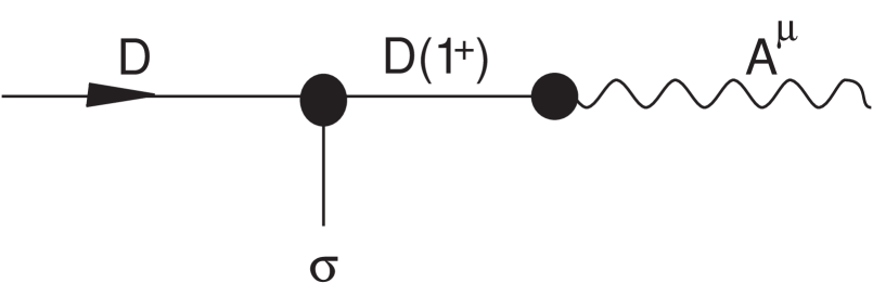
FIG. 1.: Diagram for the polar contribution to the $D\to\sigma$ semileptonic amplitude.

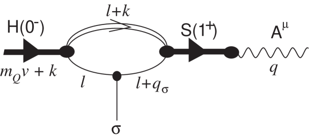
FIG. 2.: The CQM loop diagram for the process in Fig. 1. $H$ and $S$ are the heavy meson fields of Heavy-Quark-Effective-Theory, while $l$ is the momentum running in the loop. Here $H$ and $S$ coincide respectively with $D$ and $D(1^{+})$. The residual momentum carried by the $S$ field is $k^{\prime}$ while its four velocity is still $v$ since no external current is acting on the heavy quark line (the doubled one).
The weak current $A^{\mu}$ could be directly attached to the loop (i.e., without an intermediate $S$ state). This kind of contribution to the form factors, is shown in Fig. 3.

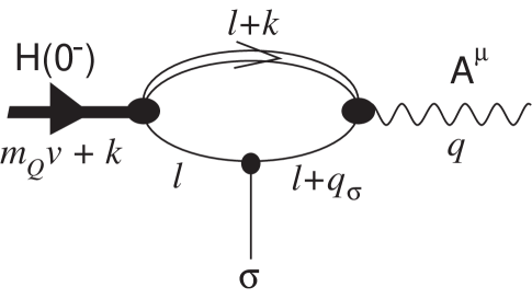
FIG. 3.: Diagram for the direct contribution to the $D\to\sigma$ semileptonic amplitude.

REFERENCES

• [1] D.E. Groom et al. (Particle Data Group) E.P.J. C15 2000 1. See also N.A. TΓΆrnqvist and M. Roos , Phys. Rev. Lett. 76 1575 (1996).
• [2] Conference: β€œPossible existence of the light $\sigma$ resonance and its implications to hadron physics”, Kyoto, Japan, June 11-14, 2000, (proceedings to appear); N.A. TΓΆrnqvist, Summary talk of the conference, hep-ph/0008135.
• [3] E. M. Aitala et al. (E791 collaboration) Experimental evidence for a light and broad scalar resonance in $D^{+}\to\pi^{-}\pi^{+}\pi^{+}$ decay, hep-ex/0007028.
• [4] A.D. Polosa, The CQM model, hep-ph/0004183 and references therein; see also A. Deandrea, N. Di Bartolomeo, R. Gatto, G. Nardulli and A.D. Polosa, Phys. Rev. D58, 034004 (1998); A. Deandrea, R. Gatto, G. Nardulli and A.D. Polosa, ibid. 59, 074012 (1999); A.D. Polosa, in Proceedings of 11th Rencontres de Blois: Frontiers of Matter, Chateau de Blois, France, hep-ph/9909371.
• [5] A. Manohar and M. Wise, Heavy Quark Physics, Cambridge, 2000.
• [6] M.M. Zoeller (CLEO collaboration), talk at American Physical Society DPF’99,
http://www.physics.ucla.edu/dpf99/trans/3-16.pdf.
• [7] A. Deandrea, R. Gatto, G. Nardulli and A.D. Polosa, Phys. Rev. 61, 017502 (2000).
• [8] D. Ebert and M.K. Volkov, Z. Phys. C16, 205 (1983); D. Ebert, Bosonization in Particle Physics, hep-ph/9710511.
• [9] C. Dib and R. Rosenfeld, Estimating $\sigma$ meson couplings from $D\to 3\pi$ decays, hep-ph/0006145; see also A.D. Polosa, N.A. TΓΆrnqvist, M.D. Scadron and V. Elias, Weak Interaction Evidence for a Broad $\sigma(500-600)$ Resonance, hep-ph/0005106.
• [10] M. Bauer, B. Stech and M. Wirbel, Z. Phys. C34, 103 (1987).
• [11] R. Casalbuoni et al., Phys. Rep. 281, 145 (1997).
Refer to caption