The Renormalization Group Improvement of the QCD Static Potentials

Abstract

We resum the leading ultrasoft logs of the singlet and octet static QCD potentials within potential NRQCD. We then obtain the complete three-loop renormalization group improvement of the singlet QCD static potential. The discrepancies between the perturbative evaluation and the lattice results at short distances are slightly reduced.

PACS numbers: 12.38.Cy, 12.38.Bx, 12.39.Hg

Recently, there has been quite a lot of effort in identifying the large logs that arise from the different scales involved in heavy quark systems near threshold [1, 2, 3, 4, 5, 6, 7]. The proper renormalization group (RG) resummation of these logs is a non-trivial issue. It has recently been addressed within the so-called vNRQCD approach [8] for the $O(1/m^{2})$ potentials [9], and for the $O(1/m)$ potential and the production current [10]. Since the proper resummation of the logs may be important for the physics of the top quark production near threshold, as well as for heavy quarkonium systems, and the existing calculations (see [2]) are done in a formalism closer to potential NRQCD (pNRQCD) [11, 4], it would be desirable to know how to RG-improve within the latter formalism. In this note we provide the first step towards this goal by showing how the static potentials of QCD can be RG-improved within that framework. Moreover, the RG-improved static potentials obtained in this paper represent a new result by themselves. They provide the complete three-loop RG evolution of the static potentials within an expansion in $\alpha_{\rm s}$ (in order to be so, besides our calculation, one needs to know the static potentials at two loops [12, 13]). Our results may also be relevant in order to understand the discrepancies, at relatively short distances, between the perturbative evaluation and the lattice results.

Since we are only interested in the static potentials, we only need to consider the static limit of NRQCD [14] and pNRQCD, i.e. we only need to work at leading order in $1/m$. The matching between NRQCD and pNRQCD in the static limit, in the situation where $\Lambda_{\rm QCD}\ll 1/r$ (the limit we will consider in this paper), has been worked out in detail in ref. [4].

The pNRQCD lagrangian at leading order in $1/m$ and next-to-leading order in the multipole expansion reads

$${\cal L}_{\rm pNRQCD}={\rm Tr}\,\Biggl{\{}{\rm S}^{\dagger}\left(i\partial_{0}-V_{s}\right){\rm S}+{\rm O}^{\dagger}\left(iD_{0}-V_{o}\right){\rm O}\Biggr{\}}$$

$$\qquad+gV_{A}(r){\rm Tr}\left\{{\rm O}^{\dagger}{\bf r}\cdot{\bf E}\,{\rm S}+{\rm S}^{\dagger}{\bf r}\cdot{\bf E}\,{\rm O}\right\}+g{V_{B}(r)\over 2}{\rm Tr}\left\{{\rm O}^{\dagger}{\bf r}\cdot{\bf E}\,{\rm O}+{\rm O}^{\dagger}{\rm O}{\bf r}\cdot{\bf E}\right\}$$

$$\qquad-{1\over 4}F_{\mu\nu}^{a}F^{\mu\nu\,a}+O(r^{2})\,.$$ (1)

All the gauge fields in Eq. (1) are evaluated in ${\bf R}$ and $t$, in particular $F^{\mu\nu\,a}\equiv F^{\mu\nu\,a}({\bf R},t)$ and $iD_{0}{\rm O}\equiv i\partial_{0}{\rm O}-g[A_{0}({\bf R},t),{\rm O}]$ and

$$V_{s}=-C_{f}{\alpha_{V_{s}}\over r}$$

$$V_{o}=\left({C_{A}\over 2}-C_{f}\right){\alpha_{V_{o}}\over r}.$$

The potentials $V_{i}$, $i=s,o,A,B$ are to be regarded as matching coefficients, which depend on the scale $\nu$ separating soft gluons from ultrasoft ones. In the static limit, we understand by soft energies the ones of $O(1/r)$ and by ultrasoft energies the ones of $O(\alpha_{\rm s}/r)$. Notice that the hard scale, $m$, plays no role in the static limit. The only assumption made so far concerning the size of $r$ is that $1/r\gg\Lambda_{\rm QCD}$. However, in order to use perturbative RG techniques, we shall also assume from now on that we are working at scales $\nu$ such that $\alpha_{\rm s}(\nu)\ll 1$.

Formally, we can write Eq. (1) as an expansion in $r$ in the following way:

$${\cal L}_{\rm pNRQCD}=\sum_{n=-1}^{\infty}r^{n}\lambda_{n}^{B}O_{n}^{B},$$ (2)

where the above fields and parameters should be understood as bare and the renormalization group equations of the renormalized matching coefficients read

$$\nu{d\over d\nu}\lambda=B_{\lambda}(\lambda).$$ (3)

If $\lambda_{-1}=0$, there are no relevant operators (superrenormalizable terms) in the Lagrangian and the RG equations have a triangular structure (the standard structure one can see, for instance, in HQET [15]; see Ref. [16] for a review):

$$\nu{d\over d\nu}\lambda_{0}=B_{0}(\lambda_{0})$$ (4)

$$\nu{d\over d\nu}\lambda_{1}=B_{1}(\lambda_{0})\lambda_{1}$$ (5)

$$\nu{d\over d\nu}\lambda_{2}=B_{2,(2,1)}(\lambda_{0})\lambda_{2}+B_{2,(1,2)}(\lambda_{0})\lambda_{1}^{2}$$ (6)

$$....\,,$$ (7)

where the different B’s can be power-expanded in $\lambda_{0}$ ($\lambda_{0}$ corresponds to the marginal operators (renormalizable interactions)). If $\lambda_{-1}\not=0$, however, there are relevant operators (superrenormalizable terms) in the Lagrangian and the RG equations lose the triangular structure. Still, if $\lambda_{-1}\ll 1$, a perturbative calculation of the renormalization group equations can be achieved as a double expansion in $\lambda_{-1}$ and $\lambda_{0}$. The RG equations now have the following structure:

$$\nu{d\over d\nu}\lambda_{-1}$$ (8)

$$\quad=B_{-1}(\lambda_{0})\lambda_{-1}+B_{(-1,2)}(\lambda_{0})\lambda_{-1}^{2}\lambda_{1}+B_{(-1,3)}^{(a)}(\lambda_{0})\lambda_{-1}^{3}\lambda_{1}^{2}+B_{(-1,3)}^{(b)}(\lambda_{0})\lambda_{-1}^{3}\lambda_{2}+O(\lambda_{-1}^{4})$$

$$\nu{d\over d\nu}\lambda_{0}=B_{0}(\lambda_{0})+B_{0,1}(\lambda_{0})\lambda_{-1}\lambda_{1}+O(\lambda_{-1}^{2})$$ (9)

$$\nu{d\over d\nu}\lambda_{1}=B_{1}(\lambda_{0})\lambda_{1}+B_{1,1}(\lambda_{0})\lambda_{-1}\lambda_{1}^{2}+O(\lambda_{-1}^{2})$$ (10)

and so on (for a similar discussion in the context of scalar $\lambda\phi^{n}$-like theories see [17]).

At short distances, the static limit of pNRQCD lives in the second situation. Specifically, we have $\lambda_{-1}=\{\alpha_{V_{s}},\alpha_{V_{o}}\}$, that fulfils $\lambda_{-1}\ll 1$; $\lambda_{0}=\alpha_{s}$ and $\lambda_{1}=\{V_{A},V_{B}\}$. Therefore, we can calculate the anomalous dimensions order by order in $\alpha_{\rm s}$. In addition, we also have an expansion in $\lambda_{-1}$ that corresponds to working order by order in the multipole expansion.

The specific form of the pNRQCD lagrangian severely constrains the above general structure. From ref. [4] we obtain at leading, non-vanishing, order

$$\nu{d\over d\nu}\alpha_{V_{s}} = {2\over 3}{\alpha_{s}\over\pi}V_{A}^{2}\left(\left({C_{A}\over 2}-C_{f}\right)\alpha_{V_{o}}+C_{f}\alpha_{V_{s}}\right)^{3}+O(\lambda_{-1}^{4}\lambda_{0},\lambda_{0}^{2}\lambda_{-1}^{3})$$

$$\nu{d\over d\nu}\alpha_{V_{o}} = {2\over 3}{\alpha_{s}\over\pi}V_{A}^{2}\left(\left({C_{A}\over 2}-C_{f}\right)\alpha_{V_{o}}+C_{f}\alpha_{V_{s}}\right)^{3}+O(\lambda_{-1}^{4}\lambda_{0},\lambda_{0}^{2}\lambda_{-1}^{3})$$

$$\nu{d\over d\nu}\alpha_{s} = \alpha_{s}\beta(\alpha_{s})$$

$$\nu{d\over d\nu}V_{A} = 0+O(\lambda_{-1}\lambda_{0},\lambda_{0}^{2})$$ (11)

$$\nu{d\over d\nu}V_{B} = 0+O(\lambda_{-1}\lambda_{0},\lambda_{0}^{2})\,.$$

It is the aim of this work to solve Eq. (The Renormalization Group Improvement of the QCD Static Potentials), and hence to provide the leading log (LL) ultrasoft RG improvement of the pNRQCD lagrangian in the static limit.

The last two equations in Eq. (The Renormalization Group Improvement of the QCD Static Potentials) are decoupled from the rest and are equal to zero at the order we are working. Therefore, we immediately obtain

$$V_{A}(\nu)=V_{A}({r})\qquad{\rm and}\qquad V_{B}(\nu)=V_{B}({r}).$$ (12)

The first two equations of Eq. (The Renormalization Group Improvement of the QCD Static Potentials) are equivalent to

$$\nu{d\over d\nu}\left(\left({C_{A}\over 2}-C_{f}\right)\alpha_{V_{o}}+C_{f}\alpha_{V_{s}}\right) = \gamma_{os}{\alpha_{s}\over\pi}V_{A}^{2}\left(\left({C_{A}\over 2}-C_{f}\right)\alpha_{V_{o}}+C_{f}\alpha_{V_{s}}\right)^{3}$$

$$\nu{d\over d\nu}\left(\alpha_{V_{o}}-\alpha_{V_{s}}\right) = 0,$$ (13)

where

$$\gamma_{os}={C_{A}\over 3}.$$ (14)

The second equation tells us that the combination $\alpha_{V_{o}}-\alpha_{V_{s}}$ is RG-invariant at this order. The first equation can now be easily solved (note that in order to solve these equations with the demanded accuracy it was necessary to know the RG solution of $V_{A}$, which happened to be trivial). We obtain (where $\beta_{0}=11C_{A}/3-4T_{F}n_{f}/3$, $T_{F}=1/2$ and $n_{f}$ is the number of light quarks):

$$\alpha_{V_{s}}(\nu) = \alpha_{V_{s}}(r)-{2\over 3\gamma_{os}}\left(\left({C_{A}\over 2}-C_{f}\right)\alpha_{V_{o}}(r)+C_{f}\alpha_{V_{s}}(r)\right)$$

$$\times\left(1-{1\over\sqrt{1-{4\gamma_{os}\over\beta_{0}}\left(\left({C_{A}\over 2}-C_{f}\right)\alpha_{V_{o}}(r)+C_{f}\alpha_{V_{s}}({r})\right)^{2}V_{A}^{2}({r})\log\left(\alpha_{s}({r})\over\alpha_{s}(\nu)\right)}}\right)$$

$$\alpha_{V_{o}}(\nu) = \alpha_{V_{o}}(r)-{2\over 3\gamma_{os}}\left(\left({C_{A}\over 2}-C_{f}\right)\alpha_{V_{o}}(r)+C_{f}\alpha_{V_{s}}(r)\right)$$

$$\times\left(1-{1\over\sqrt{1-{4\gamma_{os}\over\beta_{0}}\left(\left({C_{A}\over 2}-C_{f}\right)\alpha_{V_{o}}(r)+C_{f}\alpha_{V_{s}}({r})\right)^{2}V_{A}^{2}({r})\log\left(\alpha_{s}({r})\over\alpha_{s}(\nu)\right)}}\right),$$

which completes our results. These are exact up to $O\left(\lambda_{-1}^{3}(r)\left(\lambda_{-1}^{2}(r)\left(\lambda_{0}(r)\log{r\nu}\right)^{n}\right)^{m},\right.\\ \left.\lambda_{-1}(r)\lambda_{0}(r)\left(\lambda_{-1}^{2}(r)\left(\lambda_{0}(r)\log{r\nu}\right)^{n}\right)^{m}\right)$ where $n=0,1,2...$ and $m=1,2...\,$. At this point we would like to stress the simplicity of the calculation, which follows to a large extent from the formalism used.

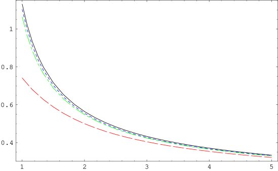
Figure 1: We plot $\alpha_{V_{s}}$ versus $r$ (GeV) for a range of energies relevant to a comparison with lattice simulations and also to the study of the $\Upsilon(1S)$ system ($n_{f}=4$, $\Lambda_{\rm QCD}^{{\rm three\,loops}}=0.28$ GeV). The solid line corresponds to $\alpha^{{\rm(2\,loops)}}_{V_{s}}$, the dotted line to $\alpha_{V_{s}}^{{\rm(2\,loops)}}$ plus the single leading-log correction computed in Ref. [3], the dot-dashed line to Eq. (16) and the dashed line to Eq. (The Renormalization Group Improvement of the QCD Static Potentials). We have fixed $\nu=\alpha_{\rm s}(r)/r$.

In the above results the different matching coefficients can be considered to be independent (though assuming $\lambda_{-1}$, $\lambda_{0}\ll 1$ in order for our perturbative evaluation to make sense). If we want to perform a strict expansion in $\alpha_{\rm s}$, one has to use the perturbative relation between $\lambda_{-1}(r)$, $\lambda_{1}(r)$ and $\alpha_{\rm s}(r)$: $\lambda_{-1}(r)=A_{1}\alpha_{\rm s}(r)+A_{2}\alpha_{\rm s}^{2}(r)+...$ and $\lambda_{1}(r)=1+B_{1}\alpha_{\rm s}(r)+...$. Since $\alpha_{V_{s}}$ and $\alpha_{V_{o}}$ are known at two-loop accuracy [12, 13], Eq. (The Renormalization Group Improvement of the QCD Static Potentials) is known with the following accuracy

$$\alpha_{V_{s}}(\nu) = \alpha_{V_{s}}^{(2\,{\rm loops})}({r})+{C_{A}^{3}\over 6\beta_{0}}\alpha_{\rm s}^{3}(r)\log\left(\alpha_{s}({r})\over\alpha_{s}(\nu)\right)+O(\alpha_{\rm s}(r)^{4+n}\log^{n}{r\nu})$$ (16)

$$\alpha_{V_{o}}(\nu) = \alpha_{V_{o}}^{(2\,{\rm loops})}({r})+{C_{A}^{3}\over 6\beta_{0}}\alpha_{\rm s}^{3}(r)\log\left(\alpha_{s}({r})\over\alpha_{s}(\nu)\right)+O(\alpha_{\rm s}(r)^{4+n}\log^{n}{r\nu}),$$

where $n=0,1,2,...\,$.

The above equation represents the complete three-loop RG improvement of the static potentials. When the running $\alpha_{s}(r)$ is substituted by its three-loop expression above and expanded, all the $\log r\nu$ in the three-loop static potentials are obtained, including the infrared logs of [18, 3]. More explicitly, if we write $\lambda_{-1}=\lambda_{-1}(r,\nu,\alpha_{\rm s}(\nu))$, Eq. (16) provides the correct $\alpha_{\rm s}^{1+n}(\nu)\log^{n}{r\nu}$, $\alpha_{\rm s}^{2+n}(\nu)\log^{n}{r\nu}$, $\alpha_{\rm s}^{3+n}(\nu)\log^{n}{r\nu}$ terms at any power of $n$. Note that such accuracy is not achieved by only replacing $\alpha_{s}(r)$ by its three-loop running expression in the two-loop calculation of the potential, as it is sometimes done in the literature [19] (see also [20]).

The Lagrangian (1) is suitable for the study of static systems. In particular, we may be interested in computing the energy of two infinitely heavy (static) sources separated at a distance $r$ in a singlet configuration. This is, indeed, the object computed in lattice simulations and usually referred as the static potential. Within our formalism, this energy corresponds to the pole of the singlet-singlet correlator. In the energy, the scale dependence $\nu$ of $V_{s}$ gets cancelled by ultrasoft contributions of $O(\alpha_{\rm s}(r)/r)$. Therefore, by lowering the scale $\nu$ in $V_{s}$ to values of $O(\alpha_{\rm s}(r)/r)$, all the large logs arising from the ratio between the soft and ultrasoft scale are resummed and the energy becomes, at the accuracy we are working, equal to $V_{s}$ with $\nu=\alpha_{\rm s}(r)/r$ (up to finite terms). Now we would like to give some numerical estimates of our results (we fix $\nu=\alpha_{\rm s}(r)/r$ in what follows). In Fig. 1, we plot $\alpha_{V_{s}}$ versus $r$ (GeV), within different approximations. If we compare the last term in Eq. (16) with the single leading-log result obtained in [3], we can see a sizeable correction of the same order of magnitude. If for definiteness we choose $r^{-1}=2\,{\rm GeV}$, Eq. (16) gives a correction of around 3%, whereas the single leading-log term gives a correction of around 1%. This shows the necessity to RG-improve the single leading logs. In any case, as we can see from Fig. 1 and the above results, the correction is rather tiny whith respect to the total value of $\alpha_{V_{S}}$. Equation (The Renormalization Group Improvement of the QCD Static Potentials), however, produces a much more sizeable correction, as we can see in Fig. 1. If we again take $r^{-1}=2\,{\rm GeV}$ the correction is of around 11%.

In all the cases the new results lower the value of $\alpha_{V_{s}}$, reducing the existing discrepancies between the perturbative results and the lattice simulations [21]. This is specially so when using Eq. (The Renormalization Group Improvement of the QCD Static Potentials). Although the good behaviour of $\alpha_{V_{s}}$ using Eq. (The Renormalization Group Improvement of the QCD Static Potentials) is certainly appealing, we should bear in mind that around the $1\,{\rm GeV}$ region $\lambda_{-1}(r)\sim 1$ and hence perturbation theory becomes unreliable. This is so specially in the perturbative relation between $\alpha_{V_{s}}(r)$ and $\alpha_{\rm s}(r)$ and it is usually associated to renormalon effects [22]. This point should be better understood before a detailed study about the impact of the RG improvement can be done.

Since for $\alpha_{V_{o}}(r)$ only the one-loop expression is available, we refrain from performing a similar study for it (note that in the numerical analysis above we have used the one-loop expression of $\alpha_{V_{o}}(r)$ in Eq. (The Renormalization Group Improvement of the QCD Static Potentials)).

One could also consider non-perturbative effects in the static case when $1/r\gg\Lambda_{\rm QCD}$ (see [4] for a more general discussion). Here we only mention that when $\alpha_{s}(r)/r\gg\Lambda_{\rm QCD}$ the leading non-perturbative contribution is proportional to $r^{3}\langle\alpha_{s}FF\rangle/\alpha_{s}(r)$ [24], whereas for $\alpha_{s}(r)/r\sim\Lambda_{\rm QCD}$ one has a non-perturbative contribution proportional to $r^{2}$ times a non-local correlator of two chromoelectric fields with multiple potential insertions of $O(\alpha_{\rm s}(r)/r)$.

Our results are also relevant to actual physical systems composed of a quark and an antiquark with very large but finite mass. However, in order to achieve, for instance, an $O(m\alpha_{\rm s}^{4+n}\log^{n}\alpha_{\rm s})$ accuracy in the binding energy of those systems, the RG improvement of the $1/m$ and $1/m^{2}$ potentials is also necessary. Since local field redefinitions allow to reshuffle contributions from a given order in $1/m$ to another [23], a meaningful outcome can only be obtained when all the contributions from the various potentials are taken into account. Hence, we restrict ourselves here to present a few numerical estimates on the impact of the RG-improved static potentials for some typical scales one can find in the $\Upsilon(1S)$ and $t$-$\bar{t}$ systems. In particular, for the $\Upsilon(1S)$, for which typical soft scales are of $O(2\,{\rm GeV})$, the discussion of Fig. 1 applies. For $t$-$\bar{t}$ systems, in order to give an estimate, we take $r^{-1}=20\,{\rm GeV}$ ($n_{f}=5$, $\Lambda_{\rm QCD}^{{\rm three\,loops}}=0.2$). We obtain that the corrections are of order 0.4%, 0.5%, 1%, if we consider the single leading-log result, Eq. (16) and Eq. (The Renormalization Group Improvement of the QCD Static Potentials), respectively.

Before closing, let us mention that in the vNRQCD approach it appears to be crucial that ultrasoft and soft gluons run from a scale $mv^{2}$ and $mv$, respectively, to the scale $m$. In the static system, the scale $m$ does not exist, and hence it is not clear to us how one should proceed in the above-mentioned approach. Notice also that the difficulties pointed out in [25] concerning a naïve RG improvement in two stages do not apply to the static case, since here only one stage is involved, namely the RG improvement between NRQCD and pNRQCD.

Acknowledgements

We thank M. Beneke, J. Kuti, A. Manohar, I. Stewart and A. Vairo for stimulating discussions. We also thank G. Bali for sharing his lattice data with us. A.P. acknowledges the TMR contract No. ERBFMBICT983405 and J.S. the financial support from the CICYT (Spain), contract AEN98-0431, the CIRIT (Catalonia), contract 1998SGR 00026, and the grant BGP-08 (Catalonia). J. S. thanks A. Manohar and the HEP group at UCSD for their warm hospitality while this work was carried out.

References

• [1] M. Beneke, A. Signer and V.A. Smirnov, Phys. Rev. Lett. 80 (1998) 2535; A. Czarnecki and K. Melnikov, Phys. Rev. Lett. 80 (1998) 2531.
• [2] A.H. Hoang, M. Beneke, K. Melnikov, T. Nagano, A. Ota, A.A. Penin, A.A. Pivovarov, A. Signer, V.A. Smirnov, Y. Sumino, T. Teubner, O. Yakovlev and A. Yelkhovsky, Eur. Phys. J. direct C 3 (2000) 1.
• [3] N. Brambilla, A. Pineda, J. Soto and A. Vairo, Phys. Rev. D 60 (1999) 091502.
• [4] N. Brambilla, A. Pineda, J. Soto and A. Vairo, Nucl. Phys. B 566 (2000) 275.
• [5] B. A. Kniehl and A. A. Penin, Nucl. Phys. B 563 (1999) 200.
• [6] N. Brambilla, A. Pineda, J. Soto and A. Vairo, Phys. Lett. B 470 (1999) 215.
• [7] B. A. Kniehl and A. A. Penin, hep-ph/9911414.
• [8] M. E. Luke, A. V. Manohar and I. Z. Rothstein, Phys. Rev. D 61 (2000) 074025.
• [9] A. V. Manohar and I. W. Stewart, hep-ph/9912226; hep-ph/0003032.
• [10] A. V. Manohar and I. W. Stewart, hep-ph/0003107.
• [11] A. Pineda and J. Soto, Nucl. Phys. Proc. Suppl. 64 (1998) 428.
• [12] Y. SchrΓΆder, Phys. Lett. B 447 (1999) 321; M. Peter, Nucl. Phys. B 501 (1997) 471.
• [13] Y. SchrΓΆder, private communication.
• [14] W. E. Caswell and G. P. Lepage, Phys. Lett. B 167 (1986) 437; G.T. Bodwin, E. Braaten and G.P. Lepage, Phys. Rev. D 51 (1995) 1125, Erratum ibid. D 55 (1997) 5853.
• [15] S. Balk, J.G. Korner and D. Pirjol, Nucl. Phys. B 428 (1994) 499; C. Bauer and A. V. Manohar, Phys. Rev. D 57 (1998) 337; C. Balzereit, Phys. Rev. D 59 (1999) 034006.
• [16] M. Neubert, Phys. Rep. 245 (1994) 259.
• [17] M. Atance and J. L. Cortes, Phys. Rev. D 56 (1997) 3611.
• [18] T. Appelquist, M. Dine and I. J. Muzinich, Phys. Rev. D 17 (1978) 2074.
• [19] M. Peter, Phys. Rev. Lett. 78 (1997) 602.
• [20] V. V. Kiselev, A. E. Kovalsky and A. I. Onishchenko, hep-ph/0005020.
• [21] G.Β S.Β Bali and K.Β Schilling, Phys.Β Rev.Β  D47 (1993) 661; G.Β S.Β Bali and K.Β Schilling, Int.Β J.Β Mod.Β Phys.Β  C4 (1993) 1167; G.Β S.Β Bali, K.Β Schilling and A.Β Wachter, Phys.Β Rev.Β  D56 (1997) 2566; K. J. Juge, J. Kuti and C.J. Morningstar, hep-lat/9911007.
• [22] M. Jezabek, J.H. Kuhn, M. Peter, Y. Sumino and T. Teubner, Phys. Rev. D 58 (1998), 014006; M. Jezabek, M. Peter and Y. Sumino, Phys. Lett. B 428 (1998) 352.
• [23] N. Brambilla, A.Pineda, J. Soto and A. Vairo, hep-ph/0002250.
• [24] C.A. Flory, Phys. Lett. B 113 (1982) 263; R.A. Bertlmann and J.S. Bell, Nucl. Phys. B 227 (1983) 435.
• [25] A. V. Manohar, J. Soto and I. W. Stewart, hep-ph/0006096.