July 2000

Cavendish-HEP-00/04

BICOCCA-FT-00-11

Non-perturbative effects in the W and Z transverse momentum distribution

A. Guffanti

Dipartimento di Fisica, Università di Milano-Bicocca,

Via Celoria 16, 20133 Milano, Italy.

and

G.E. Smye

Cavendish Laboratory, University of Cambridge,

Madingley Road, Cambridge CB3 0HE, U.K.

Abstract

We use the “dispersive method” to investigate non-perturbative effects in the transverse momentum distribution of vector bosons produced in $p\bar{p}$ collisions. The assumption of a non-perturbative modification to the running coupling at low scales leads to additional contributions in impact parameter space proportional to $-b^{2}\log Q^{2}$ and $-b^{2}$. Our results, which we expect to be valid provided $\tau$ is not close to 1, are shown to account for a substantial proportion of the total non-perturbative contribution extracted from data.

1 Introduction

The measured transverse momentum distributions of W and Z bosons at the Tevatron and LHC will provide great insights into the structure of hadrons. Indeed some very interesting data has already been released [1]. On the theoretical side, the application of perturbation theory has led to a full next-to-leading order calculation [2] and next-to-leading log resummations [3, 4, 5, 6]. These are merged to give what is at present our best perturbative prediction for the distribution. There are two different approaches in the literature [3] to the resummation of these logarithms: either the contributions are resummed directly in transverse momentum space, or a Fourier transform is performed and the calculation developed in impact parameter space. These approaches were compared in [4] and shown to differ only for NNN-leading logs. In this article we will use the impact parameter formalism, since it is more readily suited to the calculation at hand. Perturbation theory has however proved insufficient to describe experimental data, and it is necessary to include in calculations large non-perturbative effects. Parametrisations of these contributions have been proposed [5], and values for parameters have been extracted from data [7, 8]; however a full theoretical understanding of these effects has yet to emerge.

One technique that has had success in describing non-perturbative effects over a wide range of QCD observables is the dispersive approach [9]. It is related to the renormalon model (see [10] for a review) but rests on slightly different foundations. The primary assumption is that one can define a universal running strong coupling $\alpha_{s}(k^{2})$ that has no singularities in the complex plane except for a branch cut along the negative real axis. In particular there is no Landau pole, which is an unphysical artefact of perturbation theory. The contribution already accounted for in a fixed-order perturbative calculation is then subtracted off, leaving what is termed the ‘non-perturbative’ correction. The assumption of universality of the running coupling, and thus of the non-perturbative parameters derived from it, is most easily tested using data from event shapes in $e^{+}e^{-}$ annihilation [11] and deep inelastic scattering [12]: these are particularly large corrections all proportional to the first moment of the non-perturbative modification to the coupling. Studies indicate that universality is approximately realised, both giving support to the model, and prompting potential refinements of some calculations [13].

Power corrections to observables in the Drell-Yan process have previously been studied using the renormalon and dispersive approaches in [14, 15, 16]. In addition, non-perturbative corrections to a calculation involving a next-to-leading log resummation were studied for the first time in the dispersive approach for the $e^{+}e^{-}$ energy-energy correlation [17]. Here we apply the same technique to the next-to-leading log resummation of the W/Z transverse momentum distribution. A simplified overview of the perturbative resummation is presented in section 2, while the power corrections to the distribution are calculated in section 3. There then follows in section 4 a discussion of the results.

2 Transverse momentum distribution

We recall the perturbative prediction for the transverse momentum distribution in two stages: first we consider the emission of a single gluon; and then we resum leading logarithms arising from multiple collinear gluon radiation, figure 1. Non-perturbative corrections from the modification to the coupling at low scales can then be added to this perturbative result.

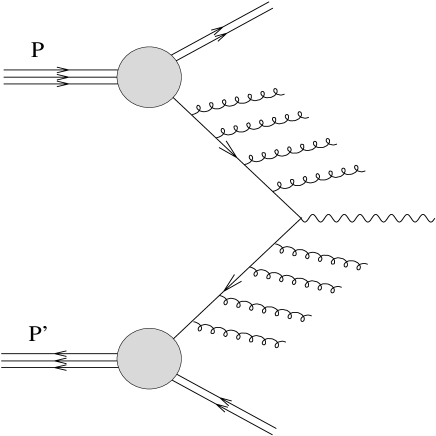
Figure 1: Vector boson production with collinear gluon emission.

2.1 Single gluon emission

Suppose in the collision of two hadrons $P$ and $P^{\prime}$, a quark and antiquark annihilate into a vector boson. The parton model gives the total cross-section for the process as

$$\sigma(\tau)=\sum_{q,\bar{q}}\int_{0}^{1}dxd{x^{\prime}}\left[q(x,\mu^{2})\bar{q}^{\prime}({x^{\prime}},\mu^{2})+\bar{q}(x,\mu^{2})q^{\prime}({x^{\prime}},\mu^{2})\right]\sigma_{q\bar{q}}(x,x^{\prime},\tau,\mu^{2})\;,$$ (2.1)

where $q$ and $\bar{q}$ are the annihilating species of quark and antiquark respectively, whose distribution functions in $P$ and $P^{\prime}$ appear above, $\sigma_{q\bar{q}}$ is the parton-level cross-section, and the standard Drell-Yan variable is

$$\tau=\frac{Q^{2}}{s}\;,$$ (2.2)

where $Q$ is the boson mass and $\sqrt{s}$ the total energy in centre-of-momentum frame. We have also explicitly introduced the factorisation scale $\mu^{2}$, which is in principle arbitrary but which (it will be seen below) is naturally chosen for the transverse momentum distribution to be $(b_{0}/b)^{2}$.

In order to find the differential ${{\bf p}_{\perp}}$ distribution $d\sigma/d^{2}{{\bf p}_{\perp}}$, where ${{\bf p}_{\perp}}$ is the two-component transverse momentum of the produced boson, normal to the incident hadron momenta, we simply insert a factor $\delta^{2}({{\bf p}_{\perp}}+\sum_{i}{{\bf k}_{\perp}}_{i})$ into the phase-space integral, where here $i$ runs over all emitted gluons. It is convenient to move into impact parameter space, writing

$$\delta^{2}({{\bf p}_{\perp}}+\sum_{i}{{\bf k}_{\perp}}_{i})=\int\frac{d^{2}{\bf b}}{(2\pi)^{2}}e^{i{\bf b}\cdot({{\bf p}_{\perp}}+\sum_{i}{{\bf k}_{\perp}}_{i})}\;.$$ (2.3)

Thus we find

$$\frac{d\sigma}{d^{2}{{\bf p}_{\perp}}}(\tau)=\int\frac{d^{2}{\bf b}}{(2\pi)^{2}}e^{i{\bf b}\cdot{{\bf p}_{\perp}}}\sum_{q,\bar{q}}\int_{0}^{1}dxd{x^{\prime}}\left[q(x,\mu^{2})\bar{q}^{\prime}({x^{\prime}},\mu^{2})+(\leftrightarrow)\right]\hat{\sigma}_{q\bar{q}}(x,{x^{\prime}},\tau,\mu^{2},b)\;,$$ (2.4)

where $\hat{\sigma}_{q\bar{q}}$ is now the cross-section calculated with an additional factor $e^{i{\bf b}\cdot{{\bf k}_{\perp}}}$ for each real emitted gluon. Performing the angular integrals then gives

$$\Sigma(\tau,p_{\perp}^{2}) \equiv \frac{d\sigma}{dp_{\perp}^{2}}(\tau)$$

$$= \frac{1}{2}\int_{0}^{\infty}db\,bJ_{0}(bp_{\perp})\sum_{q,\bar{q}}\int_{0}^{1}dxd{x^{\prime}}\left[q(x,\mu^{2})\bar{q}^{\prime}({x^{\prime}},\mu^{2})+(\leftrightarrow)\right]\hat{\sigma}_{q\bar{q}}(x,{x^{\prime}},\tau,\mu^{2},b)\;.$$

At Born level, ${\cal O}(\alpha_{s}^{0})$, we find

$$\hat{\sigma}_{q\bar{q}}^{(0)}=\frac{1}{2x{x^{\prime}}s}\frac{1}{N_{c}}\left[2\pi\delta(x{x^{\prime}}s-Q^{2})\right]\left[4\pi\alpha_{q\bar{q}}Q^{2}\right]=\frac{4\pi^{2}\alpha_{q\bar{q}}}{N_{c}s}\delta(x{x^{\prime}}-\tau)\;,$$ (2.6)

where $4\pi\alpha_{q\bar{q}}$ is the coupling of the quark $q$ and antiquark $\bar{q}$ to the vector boson, which in the case of $W$ production includes the relevant CKM matrix elements.

The ${\cal O}(\alpha_{s})$ correction comprises contributions from real and virtual gluon emission. Denoting the 4-momenta of the incoming quark and antiquark $p$ and $p^{\prime}$, that of the gluon $k$ and the vector boson $q$, we may write in the centre-of-momentum frame of the incoming quark and antiqark,

$$p=\frac{\sqrt{x{x^{\prime}}s}}{2}(1,0,0,1)\hskip 56.9055ptp^{\prime}=\frac{\sqrt{x{x^{\prime}}s}}{2}(1,0,0,-1)$$ (2.7)

and

$$k=(k^{0},k_{\perp}\cos\phi,k_{\perp}\sin\phi,k^{3})\;.$$ (2.8)

To evaluate the real contribution, we note that the squared matrix element is given by

$$e^{i{\bf b}\cdot{{\bf k}_{\perp}}}|M|^{2}=e^{i{\bf b}\cdot{{\bf k}_{\perp}}}\frac{1}{N_{c}}\left[4\pi\alpha_{q\bar{q}}\right]\left(8\pi\alpha_{s}C_{F}\right)\frac{(p\cdot q)^{2}+(p^{\prime}\cdot q)^{2}}{(p\cdot k)(p^{\prime}\cdot k)}\;,$$ (2.9)

which, in terms of the variables

$$z=\frac{\tau}{x{x^{\prime}}}\hskip 56.9055pt\Delta=\frac{k_{\perp}^{2}}{Q^{2}}\;,$$ (2.10)

may be written

$$e^{i{\bf b}\cdot{{\bf k}_{\perp}}}|M|^{2}=e^{ibQ\sqrt{\Delta}\cos\phi}\frac{4\pi}{z\Delta}\frac{8\pi^{2}\alpha_{q\bar{q}}}{N_{c}}\frac{\alpha_{s}C_{F}}{2\pi}\left[2+2z^{2}-4z\Delta\right]\;.$$ (2.11)

The Lorentz-invariant integration measure and phase space for the squared matrix elements is

$$\frac{\Theta(1-z)}{4\pi}\int_{0}^{(1-z)^{2}/(4z)}\frac{z\,d\Delta}{\sqrt{(1-z)^{2}-4z\Delta}}\int_{0}^{2\pi}\frac{d\phi}{2\pi}\;,$$ (2.12)

and thus we obtain the ${\cal O}(\alpha_{s})$ real contribution as

$$\hat{\sigma}_{q\bar{q}}^{\mbox{\scriptsize real}}=\frac{4\pi^{2}\alpha_{q\bar{q}}}{N_{c}s}\frac{\Theta(1-z)}{x{x^{\prime}}}\frac{\alpha_{s}C_{F}}{2\pi}\int_{0}^{(1-z)^{2}/(4z)}\frac{d\Delta}{\Delta}\,J_{0}(bQ\sqrt{\Delta})\frac{2+2z^{2}-4z\Delta}{\sqrt{(1-z)^{2}-4z\Delta}}\;.$$ (2.13)

This is divergent at small $\Delta$ when the gluon becomes soft or collinear with one of the incoming quarks; we will therefore find it convenient to separate this logarithmic divergence from the finite remainder.

In order to simplify the calculation we take the Mellin transform

$$\tilde{\Sigma}(N,p_{\perp}^{2})\equiv\int_{0}^{1}d\tau\,\tau^{N-1}\Sigma(\tau,p_{\perp}^{2})\;.$$ (2.14)

This yields

$$\tilde{\Sigma}(N,p_{\perp}^{2})=\frac{1}{2}\int_{0}^{\infty}db\,bJ_{0}(bp_{\perp})\sum_{q\bar{q}}\frac{4\pi^{2}\alpha_{q\bar{q}}}{N_{c}s}\left[q_{N}\bar{q}_{N}^{\prime}+\bar{q}_{N}q_{N}^{\prime}\right]\left\{1+C_{1}(N,b)-R(N,b)\right\}\;,$$ (2.15)

where in the final term on the right hand side, the 1 represents the Born level contribution, and the quantity $C_{1}-R$ the finite and divergent parts of the ${\cal O}(\alpha_{s})$ correction. The moments of the parton distributions are

$$q_{N}=\int_{0}^{1}dx\,x^{N-1}q(x)\;.$$ (2.16)

Thus we obtain for the real gluon emission:

$$C_{1}^{\mbox{\scriptsize real}}-R^{\mbox{\scriptsize real}}=\frac{\alpha_{s}C_{F}}{2\pi}\int_{0}^{\infty}\frac{d\Delta}{\Delta}J_{0}(bQ\sqrt{\Delta})\int_{0}^{1+2\Delta-2\sqrt{\Delta(1+\Delta)}}dz\,z^{N-1}\frac{2+2z^{2}-4z\Delta}{\sqrt{(1-z)^{2}-4z\Delta}}\;.$$ (2.17)

The $z$ integral may be evaluated as a series expansion in $\Delta$ (see the appendix for details) to give the collinear and soft divergences:

$$R^{\mbox{\scriptsize real}}(N,b)=\frac{\alpha_{s}C_{F}}{2\pi}\int_{0}^{1}\frac{d\Delta}{\Delta}J_{0}(bQ\sqrt{\Delta})\left\{2\log\Delta+4S_{1}(N)+\frac{2}{N}+\frac{2}{N+1}\right\}\;.$$ (2.18)

Returning now to the virtual contribution, by expressing the loop integrals as a single integral over $k_{\perp}$, we obtain

$$\hat{\sigma}_{q\bar{q}}^{\mbox{\scriptsize virt}}=\frac{4\pi^{2}\alpha_{q\bar{q}}}{N_{c}s}\delta(xx^{\prime}-\tau)\frac{\alpha_{s}C_{F}}{2\pi}\int_{0}^{\infty}\frac{d\Delta}{\Delta}{\mbox{Re}}\left\{3+\frac{2-6\Delta}{\sqrt{1-4\Delta}}\log\frac{\sqrt{1-4\Delta}-1}{\sqrt{1-4\Delta}+1}\right\}\;.$$ (2.19)

This also diverges at the lower limit, and thus for the purposes of a full ${\cal O}(\alpha_{s})$ calculation a regulator is required, such as dimensional regularisation or, as performed in section 3, a small gluon mass. But this expression is sufficient for obtaining the logarithmic divergences. The virtual contribution is separated into finite and divergent pieces according to:

$$\hat{\sigma}_{q\bar{q}}^{\mbox{\scriptsize virt}}=\frac{4\pi^{2}\alpha_{q\bar{q}}}{N_{c}s}\delta(xx^{\prime}-\tau)\left[C_{1}^{\mbox{\scriptsize virt}}-R^{\mbox{\scriptsize virt}}\right]\;,$$ (2.20)

where the collinear divergence $R$ is found by expanding the integrand in $\Delta$:

$$R^{\mbox{\scriptsize virt}}=\frac{\alpha_{s}C_{F}}{2\pi}\int_{0}^{1}\frac{d\Delta}{\Delta}\Bigl{\{}-2\log\Delta-3\Bigr{\}}\;.$$ (2.21)

Thus the sum of real and virtual divergences becomes:

$$R=\frac{\alpha_{s}C_{F}}{2\pi}\int_{0}^{Q^{2}}\frac{dk_{\perp}^{2}}{k_{\perp}^{2}}\left\{-2\left[1-J_{0}(bk_{\perp})\right]\log\frac{k_{\perp}^{2}}{Q^{2}}-3+2J_{0}(bk_{\perp})\left(2S_{1}(N)+\frac{1}{N}+\frac{1}{N+1}\right)\right\}\;.$$ (2.22)

There is a certain freedom in the choice of $R$, notably in the choice of the upper limit $k_{\perp}^{2}=Q^{2}$. But this is compensated by the finite contribution $C_{1}$, which is defined such that $C_{1}-R$ gives the full ${\cal O}(\alpha_{s})$ virtual contribution.

The radiator $R$ contains the logarithmic divergences associated with single-gluon emission. It is a non-trivial function of $N$, but can be simplified by a wise choice of factorisation scale. We begin by splitting the radiator into three pieces

$$R=R_{1}+R_{2}+R_{3}\;,$$ (2.23)

where

$$R_{1} = \frac{\alpha_{s}C_{F}}{2\pi}\int_{0}^{Q^{2}}\frac{dk_{\perp}^{2}}{k_{\perp}^{2}}\left[1-J_{0}(bk_{\perp})\right]\left(-2\log\frac{k_{\perp}^{2}}{Q^{2}}-3\right)$$ (2.24)

$$R_{2} = \frac{\alpha_{s}C_{F}}{2\pi}\int_{0}^{Q^{2}}\frac{dk_{\perp}^{2}}{k_{\perp}^{2}}\left[1-J_{0}(bk_{\perp})\right]\left(3-4S_{1}(N)-\frac{2}{N}-\frac{2}{N+1}\right)$$ (2.25)

$$R_{3} = \frac{\alpha_{s}C_{F}}{2\pi}\int_{0}^{Q^{2}}\frac{dk_{\perp}^{2}}{k_{\perp}^{2}}\left(4S_{1}(N)+\frac{2}{N}+\frac{2}{N+1}-3\right)\;.$$ (2.26)

The first two pieces may be simplified by making the de facto approximation of the Bessel function:

$$\left[1-J_{0}(bk_{\perp})\right]\approx\Theta(bk_{\perp}-b_{0})\;,$$ (2.27)

where $b_{0}=2e^{-\gamma_{E}}$ and $\gamma_{E}$ is Euler’s constant, as described more fully in the appendix. Thus

$$R_{1} = \frac{\alpha_{s}C_{F}}{2\pi}\int_{(b_{0}/b)^{2}}^{Q^{2}}\frac{dk_{\perp}^{2}}{k_{\perp}^{2}}\left(-2\log\frac{k_{\perp}^{2}}{Q^{2}}-3\right)$$ (2.28)

$$R_{2} = \frac{\alpha_{s}C_{F}}{2\pi}\int_{(b_{0}/b)^{2}}^{Q^{2}}\frac{dk_{\perp}^{2}}{k_{\perp}^{2}}\left(3-4S_{1}(N)-\frac{2}{N}-\frac{2}{N+1}\right)$$ (2.29)

The contribution $R_{3}$ is formally divergent. Using dimensional regularisation, with $4+2\eta$ dimensions, it becomes

$$R_{3}=\frac{\alpha_{s}C_{F}}{2\pi}\int_{0}^{Q^{2}}\frac{dk_{\perp}^{2}}{k_{\perp}^{2}}\frac{(4\pi\mu^{2}/k_{\perp}^{2})^{-\eta}}{\Gamma(1+\eta)}\left(4S_{1}(N)+\frac{2}{N}+\frac{2}{N+1}-3+{\cal O}(\eta)\right)$$ (2.30)

where $\mu$ is the factorisation scale which appears in the quark distributions. On application of $\overline{{\mbox{\scriptsize MS}}}$, we obtain

$$R_{3}=\frac{\alpha_{s}C_{F}}{2\pi}\int_{\mu^{2}}^{Q^{2}}\frac{dk_{\perp}^{2}}{k_{\perp}^{2}}\left(4S_{1}(N)+\frac{2}{N}+\frac{2}{N+1}-3\right)\;,$$ (2.31)

where the finite contribution arising from the ${\cal O}(\eta)$ term in equation (2.30) has been absorbed into $C_{1}$. Let us therefore choose the factorisation scale to be $\mu^{2}=(b_{0}/b)^{2}$, in order that the terms $R_{2}$ and $R_{3}$ cancel. Alternatively, since these contributions are proportional to the non-singlet anomalous dimension, starting from any factorisation scale $\mu^{2}$ the terms $R_{2}$ and $R_{3}$ may be absorbed into the parton densities by means of a scale change to $(b_{0}/b)^{2}$.

Thus the single-gluon contribution may be written as

$$\tilde{\Sigma}(N,p_{\perp}^{2}) = \frac{1}{2}\int_{0}^{\infty}db\,bJ_{0}(bp_{\perp})\sum_{q\bar{q}}\frac{4\pi^{2}\alpha_{q\bar{q}}}{N_{c}s}\left[q_{N}((b_{0}/b)^{2})\bar{q}_{N}^{\prime}((b_{0}/b)^{2})+(\leftrightarrow)\right]$$ (2.32)

$$\times\left\{1+C_{1}(N,b)-R(b)\right\}\;,$$

where the collinear and soft logarithms are represented by the radiator

$$R=\frac{\alpha_{s}C_{F}}{2\pi}\int_{(b_{0}/b)^{2}}^{Q^{2}}\frac{dk_{\perp}^{2}}{k_{\perp}^{2}}\left(-2\log\frac{k_{\perp}^{2}}{Q^{2}}-3\right)\;,$$ (2.33)

and the remaining ${\cal O}(\alpha_{s})$ contribution is to be found in $C_{1}$.

2.2 Multiple gluon emission

Consider now the case in which many gluons are emitted before the vector boson is produced. Each splitting contributes to the total transverse momentum of the event: we are interested only in the contributions from soft and collinear logarithms, which may be calculated using the collinear approximation.

Let the 4-momenta of the incident hadrons be $P$ and $P^{\prime}$. In the centre of momentum frame we may write

$$P=\frac{\sqrt{s}}{2}(1,0,0,1)\hskip 50.58878ptP^{\prime}=\frac{\sqrt{s}}{2}(1,0,0,-1)\;,$$ (2.34)

where $s$ is the total energy of the collision.

Suppose the (anti)quark in $P$ has momentum fraction $x$; and let it radiate $n$ gluons with momenta $k_{i}$, $(i=1,\cdots,n)$. We may write the Sudakov decomposition

$$k_{i}=\alpha_{i}P+\beta_{i}P^{\prime}+{{\bf k}_{\perp}}_{i}\;,$$ (2.35)

in terms of which the integration measure is

$$\int\frac{d^{4}k_{i}}{(2\pi)^{4}}\,2\pi\delta^{+}(k_{i}^{2})=\int\frac{d\alpha_{i}}{2\alpha_{i}}\frac{d^{2}{{\bf k}_{\perp}}_{i}}{(2\pi)^{3}}\;.$$ (2.36)

Let $z_{i}$ be the fraction of remaining longitudinal momentum retained by the (anti)quark at the $i$th splitting, i.e.

$$\alpha_{i} = (1-z_{i})\left(x-\sum_{j=1}^{i-1}\alpha_{j}\right)$$ (2.37)

$$z_{i} = \frac{x-\sum_{j=1}^{i}\alpha_{j}}{x-\sum_{j=1}^{i-1}\alpha_{j}}\;.$$ (2.38)

Then the collinear-divergent pieces of the squared matrix element are given by the usual splitting function:

$$|{\cal M}|_{i-1}^{2}=\frac{\alpha_{s}C_{F}}{2\pi}\int\frac{dk_{\perp i}^{2}}{k_{\perp i}^{2}}\frac{d\phi_{i}}{2\pi}\frac{dz_{i}}{z_{i}}\frac{1+z_{i}^{2}}{1-z_{i}}|{\cal M}|_{i}^{2}e^{ibk_{\perp i}\cos\phi}\;,$$ (2.39)

where $\phi_{i}$ is the azimuthal angle of the $i$th gluon. Since we are considering collinear emission, the phase space is subject to the condition $\alpha_{i}>\beta_{i}$, which translates in our approximation to

$$z<1-\frac{k_{\perp}}{Q}\;.$$ (2.40)

This boundary is not the boundary of physical phase space; rather it is imposed as part of the collinear approximation. It is necessary therefore to check that any dependence in our calculation on this limit is a genuine physical effect and not an artefact of the approximation.

We may treat radiation from the other incoming (anti)quark in the same way, but with $\alpha_{i}$ and $\beta_{i}$ interchanged. The real part of the partonic cross-section appeaing in (2.1) is then:

$$\hat{\sigma}_{q\bar{q}}^{\mbox{\scriptsize real}}=\frac{1}{2x{x^{\prime}}s}\frac{1}{N_{c}}\left[4\pi\alpha_{q\bar{q}}\tau\right]\sum_{n=0}^{\infty}\frac{1}{n!}\prod_{i=1}^{n}\left\{\frac{\alpha_{s}C_{F}}{2\pi}\int\frac{dk_{\perp i}^{2}}{k_{\perp i}^{2}}J_{0}(bk_{\perp i})\int\frac{dz_{i}}{z_{i}}\frac{1+z_{i}^{2}}{1-z_{i}}\right\}\times$$

$$\sum_{n^{\prime}=0}^{\infty}\frac{1}{n^{\prime}!}\prod_{i^{\prime}=1}^{n^{\prime}}\left\{\frac{\alpha_{s}C_{F}}{2\pi}\int\frac{dk_{\perp i^{\prime}}^{\prime 2}}{k_{\perp i^{\prime}}^{\prime 2}}J_{0}(bk_{\perp i^{\prime}}^{\prime})\int\frac{dz_{i^{\prime}}^{\prime}}{z_{i^{\prime}}^{\prime}}\frac{1+z_{i^{\prime}}^{\prime 2}}{1-z_{i^{\prime}}^{\prime}}\right\}\,2\pi\delta(x{x^{\prime}}z_{1}\cdots z_{n}z_{1}^{\prime}\cdots z_{n^{\prime}}^{\prime}-\tau)\;.$$

Taking the Mellin transform leads to:

$$\tilde{\Sigma}(N,p_{\perp}^{2})=\frac{1}{2}\int_{0}^{\infty}db\,bJ_{0}(bp_{\perp})\sum_{q\bar{q}}\frac{4\pi^{2}\alpha_{q\bar{q}}}{N_{c}s}\left[q_{N}\bar{q}_{N}^{\prime}+\bar{q}_{N}q_{N}^{\prime}\right]e^{-R(N,b)}\;,$$ (2.42)

where the real emission radiator is

$$R_{\mbox{\scriptsize real}}(N,b)=-\frac{\alpha_{s}C_{F}}{\pi}\int_{0}^{Q^{2}}\frac{dk_{\perp}^{2}}{k_{\perp}^{2}}J_{0}(bk_{\perp})\int_{0}^{1-k_{\perp}/Q}dz\,z^{N-1}\frac{1+z^{2}}{1-z}\;.$$ (2.43)

We then take into account virtual gluon radiation using the universal virtual contribution to the radiator [17]

$$R_{\mbox{\scriptsize virtual}}(b)=\frac{\alpha_{s}C_{F}}{\pi}\int_{0}^{Q^{2}}\frac{dk_{\perp}^{2}}{k_{\perp}^{2}}\int_{0}^{1-k_{\perp}/Q}dz\frac{1+z^{2}}{1-z}\;,$$ (2.44)

so that the full radiator is

$$R(N,b)=\frac{\alpha_{s}C_{F}}{\pi}\int_{0}^{Q^{2}}\frac{dk_{\perp}^{2}}{k_{\perp}^{2}}\int_{0}^{1-k_{\perp}/Q}dz\frac{1+z^{2}}{1-z}\left[1-z^{N-1}J_{0}(bk_{\perp})\right]\;.$$ (2.45)

Performing the $z$ integral at small $k_{\perp}^{2}$ yields:

$$R(N,b)=\frac{\alpha_{s}C_{F}}{2\pi}\int_{0}^{Q^{2}}\frac{dk_{\perp}^{2}}{k_{\perp}^{2}}G(k_{\perp}^{2}/Q^{2},bk_{\perp},N)\;.$$ (2.46)

where

$$G(k_{\perp}^{2}/Q^{2},bk_{\perp},N) = -2\left[1-J_{0}(bk_{\perp})\right]\log\frac{k_{\perp}^{2}}{Q^{2}}-3+2J_{0}(bk_{\perp})\left(2S_{1}(N)+\frac{1}{N}+\frac{1}{N+1}\right)$$ (2.47)

$$\hskip 56.9055pt+4\left[1-NJ_{0}(bk_{\perp})\right]\frac{k_{\perp}}{Q}+{\cal O}\left(\frac{k_{\perp}^{2}}{Q^{2}}\right)\;.$$

It should be noted that:

• This result is strictly valid provided $N$ is not too large, which here means approximately $N<Q/k_{\perp}$, since as $N\to\infty$ the contribution from real emission in (2.45) vanishes. But we are not interested in such large values of $N$, since they correspond to values of $\tau$ close to $1$, while for vector boson production at the LHC or Tevatron the order of magnitude is $\tau\sim 0.01$.

• The terms of order $k_{\perp}^{2}/Q^{2}$ do not generate logarithmic divergences: they are thus included in the finite contribution to the cross-section and therefore do not feature in the radiator. The term of order $k_{\perp}/Q$ is a spurious artefact of the collinear approximation, that is not present in the single-gluon result. The collinear approximation is thus valid only for logarithm resummation, and may not be used for determinations of power corrections [15].

The decomposition of the radiator proceeds just as in the single-gluon case. The factorisation scale is naturally chosen to be $\mu^{2}=(b_{0}/b)^{2}$ and we obtain the exponentiated form:

$$\tilde{\Sigma}(N,p_{\perp}^{2})=\frac{1}{2}\int_{0}^{\infty}db\,bJ_{0}(bp_{\perp})\sum_{q\bar{q}}\frac{4\pi^{2}\alpha_{q\bar{q}}}{N_{c}s}\left[q_{N}((b_{0}/b)^{2})\bar{q}_{N}^{\prime}((b_{0}/b)^{2})+(\leftrightarrow)\right]C(\alpha_{s})e^{-R(b)}\;,$$ (2.48)

where the leading collinear and soft logarithms are represented by the radiator

$$R=\frac{\alpha_{s}C_{F}}{2\pi}\int_{(b_{0}/b)^{2}}^{Q^{2}}\frac{dk_{\perp}^{2}}{k_{\perp}^{2}}\left(-2\log\frac{k_{\perp}^{2}}{Q^{2}}-3\right)\;,$$ (2.49)

and the remaining contribution to fixed order in perturbation theory is given by the factor

$$C(\alpha_{s})=1+C_{1}(N,b)+{\cal O}(\alpha_{s}^{2})\;.$$ (2.50)

Next-to-leading logarithms have been calculated [3, 4, 5, 6], and may be included in the radiator by writing

$$R=\frac{C_{F}}{2\pi}\int_{(b_{0}/b)^{2}}^{Q^{2}}\frac{dk_{\perp}^{2}}{k_{\perp}^{2}}\alpha_{s}^{\mbox{\scriptsize PT}}(k_{\perp}^{2})\left(-2\log\frac{k_{\perp}^{2}}{Q^{2}}-3\right)\;,$$ (2.51)

where the perturbative coupling is defined in the Bremsstrahlung scheme [19], and is, to next-to-leading order,

$$\alpha_{s}^{{\mbox{\scriptsize PT}}}(k_{\perp}^{2})=\alpha_{s}^{\overline{{\mbox{\tiny MS}}}}(Q^{2})+\left[\alpha_{s}^{\overline{{\mbox{\tiny MS}}}}(Q^{2})\right]^{2}\left(\frac{\beta_{0}}{4\pi}\log\frac{Q^{2}}{k_{\perp}^{2}}+\frac{K}{4\pi}\right)\;,$$ (2.52)

where

$$K=\frac{(67-3\pi^{2})C_{A}-20T_{R}n_{f}}{9}\;.$$ (2.53)

Having now recalled the perturbative contribution to the transverse momentum distribution, we are in a position to calculate non-perturbative effects from the modification to the coupling at low scales.

3 Non-perturbative contribution

The dispersive approach to power corrections [9] has been applied to a variety of QCD observables. The basic postulate is that we may define a universal running strong coupling $\alpha_{s}(k^{2})$ that is well-behaved in the infra-red as well as in the ultra-violet, having no singularities in the complex plane apart from a branch cut along the negative real axis. We may then write a dispersion relation

$$\alpha_{s}(k^{2})=-\int_{0}^{\infty}\frac{d\mu^{2}}{k^{2}+\mu^{2}}\rho_{s}(\mu^{2})\;,$$ (3.1)

where $\rho_{s}(\mu^{2})$ is the discontinuity of $\alpha_{s}$ across its branch cut:

$$\rho_{s}(\mu^{2})=\frac{1}{2\pi i}\left\{\alpha_{s}(e^{i\pi}\mu^{2})-\alpha_{s}(e^{-i\pi}\mu^{2})\right\}\;.$$ (3.2)

Non-perturbative contributions to the transverse momentum distribution arise from the modification to the running coupling at low scales:

$$\alpha_{s}(k^{2})=\alpha_{s}^{\mbox{\scriptsize PT}}(k^{2})+\delta\alpha_{s}(k^{2})\;,$$ (3.3)

where the contribution $\alpha_{s}^{\mbox{\scriptsize PT}}$, given in (2.52), is that already accounted for in the perturbative part of the calculation. In the dispersive approach the corresponding modification to the spectral function, $\delta\rho_{s}(k^{2})$, gives the correction to the coefficient function

$$\delta C(N,b)=\frac{C_{F}}{2\pi}\int_{0}^{\infty}\frac{dk^{2}}{k^{2}}\delta\rho_{s}(k^{2})\left[{\cal C}(k^{2}/Q^{2})-{\cal C}(0)\right]$$ (3.4)

where $(\alpha_{s}C_{F}/2\pi){\cal C}(k^{2}/Q^{2})$ is just the single-gluon contribution to $C(N,b)$ calculated as though gluon has mass $k^{2}$. As customary we define $\epsilon=k^{2}/Q^{2}$.

The coefficient function has contributions from both real and virtual gluons. Consider first the real contribution. A calculation of the massive single-gluon matrix element and phase space gives

$${\cal C}^{\mbox{\scriptsize real}}=\int_{0}^{\infty}\frac{d\Delta}{\Delta}J_{0}(bQ\sqrt{\Delta})\int_{0}^{Z(\Delta,\epsilon)}dz\,z^{N-1}\frac{2\Delta(\Delta+z^{2}\Delta-2z\Delta^{2}+2\epsilon z^{2}+2\epsilon^{2}z^{2}+\epsilon^{2}z^{2}\Delta)}{(\Delta+\epsilon z)^{2}\sqrt{(1-z+\epsilon z)^{2}-4z(\epsilon+\Delta)}}$$ (3.5)

where the upper limit on the $z$ integral is

$$Z(\Delta,\epsilon)=\frac{(1+2\Delta+\epsilon)-2\sqrt{(\epsilon+\Delta)(1+\Delta)}}{(1-\epsilon)^{2}}$$ (3.6)

Note how this reduces to perturbative case (2.17) when we put $\epsilon=0$.

In order to proceed with this integral we expand the Bessel function. We require only those terms that are non-analytic in $\epsilon$ as $\epsilon\to 0$, and these are generated at the lower limit of the $\Delta$ integral. So the expansion is legitimate for our purposes and we obtain

$${\cal C}^{\mbox{\scriptsize real}}(\epsilon) = \int_{0}^{1/(1+\sqrt{\epsilon})^{2}}dz\,z^{N-1}\int_{0}^{(1-z+\epsilon z)^{2}/(4z)-\epsilon}d\Delta\left(1-\frac{b^{2}Q^{2}\Delta}{4}+\cdots\right)\times$$ (3.7)

$$\hskip 56.9055pt\frac{2(\Delta+z^{2}\Delta-2z\Delta^{2}+2\epsilon z^{2}+2\epsilon^{2}z^{2}+\epsilon^{2}z^{2}\Delta)}{(\Delta+\epsilon z)^{2}\sqrt{(1-z+\epsilon z)^{2}-4z(\epsilon+\Delta)}}\;.$$

In order to evaluate these integrals we follow the method of [9]. The integral over $\Delta$ is relatively straightforward, giving

$${\cal C}^{\mbox{\scriptsize real}}(\epsilon) = \int_{0}^{1/(1+\sqrt{\epsilon})^{2}}dz\,z^{N-1}\Biggl{[}\frac{P(z,\epsilon)}{1-z-\epsilon z}\tanh^{-1}\frac{\sqrt{(1-z-\epsilon z)^{2}-4\epsilon z^{2}}}{1-z-\epsilon z}$$ (3.8)

$$\hskip 56.9055pt-Q(z,\epsilon)\sqrt{(1-z-\epsilon z)^{2}-4\epsilon z^{2}}\Biggr{]}\;,$$

where the functions $P$ and $Q$ are given by

$$P(z,\epsilon) = 4+4(1+\epsilon)^{2}z^{2}+2\epsilon b^{2}Q^{2}z(1-z+z^{2}-\epsilon z+2\epsilon z^{2}+\epsilon^{2}z^{2})$$ (3.9)

$$Q(z,\epsilon) = 4+\frac{b^{2}Q^{2}}{6z}(1+z+z^{2}+\epsilon z+10\epsilon z^{2}+\epsilon^{2}z^{2})\;.$$ (3.10)

We then make the substitution

$$\eta=\tanh^{-1}\frac{\sqrt{(1-z-\epsilon z)^{2}-4\epsilon z^{2}}}{1-z-\epsilon z}\hskip 56.9055ptz=\frac{1}{1+\epsilon+2\sqrt{\epsilon}\cosh\eta}\;,$$ (3.11)

which leads to the expression for the characteristic function

$${\cal C}^{\mbox{\scriptsize real}}(\epsilon)=4I_{N}+2\epsilon b^{2}Q^{2}I_{N+1}+4(1+\epsilon)^{2}I_{N+2}-2\epsilon(1+\epsilon)b^{2}Q^{2}I_{N+2}+2\epsilon(1+\epsilon)^{2}b^{2}Q^{2}I_{N+3}$$ (3.12)

$$-{\textstyle\frac{2}{3}}\epsilon b^{2}Q^{2}J_{N+1}-16\epsilon J_{N+2}-{\textstyle\frac{2}{3}}\epsilon(1+\epsilon)b^{2}Q^{2}J_{N+2}-{\textstyle\frac{2}{3}}\epsilon(1+10\epsilon+\epsilon^{2})b^{2}Q^{2}J_{N+3}\;,\hskip 28.45274pt$$

in terms of the integrals

$$I_{N}(\epsilon) = \int_{0}^{\infty}d\eta\frac{\eta\tanh\eta}{(1+\epsilon+2\sqrt{\epsilon}\cosh\eta)^{N}}$$

$$J_{N}(\epsilon) = \int_{0}^{\infty}d\eta\frac{\sinh^{2}\eta}{(1+\epsilon+2\sqrt{\epsilon}\cosh\eta)^{N}}\;.$$ (3.13)

Using the values of these integrals given in the appendix, we obtain the contribution from real gluon emission as:

$${\cal C}^{\mbox{\scriptsize real}}(\epsilon) = \left\{\pi^{2}+(2S_{1}(N)+\log\epsilon)^{2}-4S_{2}(N)+2\left(\frac{1}{N}+\frac{1}{N+1}\right)(2S_{1}(N)+\log\epsilon)\right\}$$ (3.14)

$$+\frac{b^{2}Q^{2}}{6}\left(\frac{1}{N+2}-\frac{1}{N-1}\right)$$

$$+\epsilon\left\{2(2S_{1}(N)+\log\epsilon)\left(N^{2}+3N-3+\frac{1}{N+1}\right)-N\pi^{2}\right.$$

$$\hskip 56.9055pt\left.-N(2S_{1}(N)+\log\epsilon)^{2}+4NS_{2}(N)-6N^{2}-6N+16-\frac{8}{N+1}\right\}$$

$$+\frac{\epsilon b^{2}Q^{2}}{4}\left\{\pi^{2}+(2S_{1}(N)+\log\epsilon)^{2}-4S_{2}(N)+2-\frac{6}{N+2}\right.$$

$$\hskip 56.9055pt\left.+2\left(\frac{2}{N}+\frac{2}{N+2}-1\right)(2S_{1}(N)+\log\epsilon)\right\}+\cdots\;.$$

Now we turn to the virtual contribution. Since the virtual gluon does not contribute to the transverse momentum of the vector boson, we obtain the same as that calculated in [9] for the total Drell-Yan cross-section, which is

$${\cal C}^{\mbox{\scriptsize virt}} = (1+\epsilon)^{2}\left\{2{\mbox{Li}}_{2}(-\epsilon)+2\log\epsilon\log(1+\epsilon)+\frac{\pi^{2}}{3}-\log^{2}\epsilon\right\}-\frac{7}{2}-2\epsilon-(3+2\epsilon)\log\epsilon$$ (3.15)

$$= \left(-\log^{2}\epsilon-3\log\epsilon+\frac{\pi^{2}}{3}-\frac{7}{2}\right)+\epsilon\left(-2\log^{2}\epsilon+\frac{2\pi^{2}}{3}-4\right)+{\cal O}(\epsilon^{2})\;.$$

The power correction is most conveniently expressed in terms of moments of the modification to the coupling, $\delta\alpha_{s}(k^{2})$:

$$\delta C(N,b)=\frac{C_{F}}{2\pi}\int_{0}^{\infty}\frac{dk^{2}}{k^{2}}\delta\alpha_{s}(k^{2}){\cal D}(k^{2}/Q^{2})\;,$$ (3.16)

where ${\cal D}(\epsilon)$ is the discontinuity of ${\cal C}(\epsilon)$ across its branch cut:

$${\cal D}(\epsilon)=-\frac{1}{2\pi i}\left[{\cal C}(\epsilon e^{i\pi})-{\cal C}(\epsilon e^{-i\pi})\right].$$ (3.17)

The leading term in the characteristic function is the $\log\epsilon$ divergence proportional to the anomalous dimension: this is subtracted off and absorbed into the parton density functions. From the finite contribution we obtain

$${\cal D}(\epsilon) = -2\epsilon\left\{(N+2)\log\epsilon+2NS_{1}(N)-N^{2}-3N+3-\frac{1}{N+1}\right\}$$ (3.18)

$$\hskip 56.9055pt+\frac{\epsilon b^{2}Q^{2}}{2}\left\{\log\epsilon+2S_{1}(N)+\frac{2}{N}+\frac{2}{N+2}-1\right\}+\cdots\;.$$

The $b$-independent term on the first line gives the $1/Q^{2}$ corrections to the total cross-section calculated in [9]. Of particular relevance to the transverse momentum distribution is the $b$-dependent term on second line, which gives the correction

$$\delta C(N,b)=-\frac{b^{2}}{2}\left\{{\cal A}_{2}\left(\log Q^{2}-2S_{1}(N)-\frac{2}{N}-\frac{2}{N+2}+1\right)-{\cal A}_{2}^{\prime}\right\}\;.$$ (3.19)

The non-perturbative parameters ${\cal A}_{2}$ and ${\cal A}_{2}^{\prime}$ are defined in terms of $\delta\alpha_{s}$ by:

$${\cal A}_{2} = \frac{C_{F}}{2\pi}\int_{0}^{\infty}\frac{dk_{\perp}^{2}}{k_{\perp}^{2}}\,k_{\perp}^{2}\delta\alpha_{s}(k_{\perp}^{2})$$ (3.20)

$${\cal A}_{2}^{\prime} = \frac{C_{F}}{2\pi}\int_{0}^{\infty}\frac{dk_{\perp}^{2}}{k_{\perp}^{2}}\,k_{\perp}^{2}\log k_{\perp}^{2}\delta\alpha_{s}(k_{\perp}^{2})\;.$$ (3.21)

The extent of our knowledge of ${\cal A}_{2}$ and ${\cal A}_{2}^{\prime}$ is [17, 18] that ${\cal A}_{2}\approx 0.2$ GeV² and ${\cal A}_{2}^{\prime}$ is at present unconstrained but appears consistent with zero.

4 Results and discussion

In the previous section we derived the non-perturbative 1-gluon contribution to the transverse momentum distribution in impact parameter space, which by performing the inverse Mellin transform may be written:

$$\Sigma(\tau,p_{\perp}^{2})=\frac{1}{2}\int_{0}^{\infty}db\,bJ_{0}(bp_{\perp})e^{-R(b)}K(\tau,b)\left[1-b^{2}W(\tau,b)\right]$$ (4.1)

where the perturbative contribution is

$$K(\tau,b)=\sum_{q\bar{q}}\frac{4\pi^{2}\alpha_{q\bar{q}}}{N_{c}s}\int_{0}^{1}dxdx^{\prime}\left[q(x,(b_{0}/b)^{2})\bar{q}^{\prime}(x^{\prime},(b_{0}/b)^{2})+(\leftrightarrow)\right]\delta(xx^{\prime}-\tau)\;,$$ (4.2)

and the non-perturbative component is

$$W(\tau,b)=\frac{1}{2}\left\{{\cal A}_{2}\log Q^{2}+{\cal A}_{2}-{\cal A}_{2}^{\prime}\right\}-\frac{{\cal A}_{2}}{K(\tau,b)}\int_{\tau}^{1}\frac{dz}{z}K(\tau/z,b)\left(1+z^{2}-\frac{1}{(1-z)_{+}}\right)\;.$$ (4.3)

Figure 2 shows a plot of $W(\tau,b)$ against $\tau$ at fixed values of $b$, for on-shell Z⁰ production with ${\cal A}_{2}=0.2$ GeV², ${\cal A}_{2}^{\prime}=0$, evaluated using the MRST (central gluon) distributions [20]; the slight dependence of $W(\tau,b)$ on $b$ is logarithmic, coming only from the scale of the parton distributions. It is also clear from the figure that the result given here is not valid near $\tau=1$: it becomes negative and diverges logarithmically. This is because our expression for the Mellin transform was valid for $N$ not too large (equation (2.47) in the perturbative case, and analogously though not so obviously in the non-perturbative calculation), i.e. $N<Q/k_{\perp}$, while as $\tau\to 1$ the large moments become important. The approximation is valid away from this region, and is certainly legitimate for LHC or Tevatron data.

Figure 2: Graph of $W(\tau,b)$ against $\tau$ for $b=1$ GeV^-1 (solid line), $b=0.1$ GeV^-1 (dotted) and $b=0.01$ GeV^-1 (dashed), evaluated at the Z mass with ${\cal A}_{2}=0.2$ GeV² and ${\cal A}_{2}^{\prime}=0$.

We thus predict a non-perturbative correction that behaves quadratically in $b$ near $b=0$, in agreement with existing models based on a Gaussian suppression factor [5]. We can make our result Gaussian also by exponentiating:

$$1-b^{2}W(\tau,b)\approx e^{-b^{2}W(\tau,b)}\;.$$ (4.4)

Whether or not the power correction does exponentiate is an open question — intuitively it seems reasonable, since we expect contributions from all soft gluons, not just the gluon nearest the hard vertex; yet it is not proven and should be treated with care, since exponentiation normally applies to collinear and soft logarithms, while the power corrections come from terms that converge in the infra-red. Nevertheless there are several good reasons for at least studying the exponentiated correction. Firstly, the integral (4.1) diverges at large $b$ due to the non-perturbative contribution growing as $b^{2}$, while the exponentiated expression is convergent. At small $b$, where the non-perturbative correction is small, whether or not we choose to exponentiate makes minimal difference.

Secondly, we can consider the difference between the exponentiated and un-exponentiated expressions to give a measure of the theoretical uncertainty in our calculation, since we expect higher orders to contribute at approximately this level. Thus at small $b$ the error is very small, while at large $b$ it becomes huge. This has the same pattern as the general impact parameter formalism, which suffers from considerable uncertainties at large $b$ due to the parton distributions becoming unknown.

Finally, there have been some fairly reasonable phenomenological fits of Gaussian models to data, such as performed in [8]. A two-parameter fit yielded the non-perturbative contribution to the exponent

$$-b^{2}\left[0.34{\mbox{ GeV}}^{2}\log\left(\frac{Q}{1{\mbox{ GeV}}}\right)-0.16{\mbox{ GeV}}^{2}\right]\;,$$ (4.5)

while a three-parameter fit, with an additional linear term, may be written

$$-b^{2}\left[0.48{\mbox{ GeV}}^{2}\log\left(\frac{Q}{1{\mbox{ GeV}}}\right)-0.41{\mbox{ GeV}}^{2}\right]+b\left[0.09{\mbox{ GeV}}\log(100x{x^{\prime}})\right]\;.$$ (4.6)

These may be compared with the prediction from the dispersive approach, which is

$$-b^{2}W=-b^{2}\left[0.2{\mbox{ GeV}}^{2}\log\left(\frac{Q}{1{\mbox{ GeV}}}\right)-0.2{\mbox{ GeV}}^{2}\right]\;\;\;{\mbox{ at }}\;\;\;\tau=0.01\;,$$ (4.7)

where we have used ${\cal A}_{2}=0.2$ GeV² and ${\cal A}_{2}^{\prime}=0$. It is seen that this accounts for a substantial portion of the total non-perturbative function fitted to the data; however the $\tau$-dependence of the fitted forms (4.5) and (4.6) differs so greatly from that predicted here that it is hard to give more than this qualitative statement. A full fit to data is beyond the scope of this current article, but such a fit would be a further test of the dispersive model of power corrections, would enable one to extract a value for the unknown non-perturbative parameter ${\cal A}_{2}^{\prime}$, and would test the assumption of universality which predicts ${\cal A}_{2}=0.2$ GeV² from DIS structure functions [18].

An alternative approach to the non-perturbative contribution (3.19) would be to interpret part of it as a shift in the scale at which the parton distributions are evaluated. We may write the contribution as

$$\delta C(N,b)=-\frac{b^{2}{\cal A}_{2}}{2C_{F}}\gamma_{qq}(N)-\frac{b^{2}}{2}\left\{{\cal A}_{2}\left(\log Q^{2}-\frac{1}{N}+\frac{1}{N+1}-\frac{2}{N+2}-\frac{1}{2}\right)-{\cal A}_{2}^{\prime}\right\}\;,$$ (4.8)

where the non-singlet anomalous dimension is

$$\gamma_{qq}(N)=C_{F}\int_{0}^{1}dz\,z^{N-1}\left(\frac{1+z^{2}}{1-z}\right)_{+}=C_{F}\left(\frac{3}{2}-2S_{1}(N)-\frac{1}{N}-\frac{1}{N+1}\right)\;.$$ (4.9)

The first term on the right hand side of (4.8) then shifts the factorisation scale from $(b_{0}/b)^{2}$ to $(b_{0}/b)^{2}+\delta\mu^{2}$, where

$$-\frac{b^{2}{\cal A}_{2}}{2C_{F}}\gamma_{qq}(N)=2\int_{(b_{0}/b)^{2}}^{(b_{0}/b)^{2}+\delta\mu^{2}}\frac{dk_{\perp}^{2}}{k_{\perp}^{2}}\frac{\alpha_{s}(k_{\perp}^{2})}{2\pi}\gamma_{qq}(N)\;.$$ (4.10)

If as a first approximation we replace the integrand by its value at the lower limit, we obtain the shift

$$\delta\mu^{2}=-\frac{b_{0}^{2}{\cal A}_{2}}{4}\left[\frac{\alpha_{s}((b_{0}/b)^{2})C_{F}}{2\pi}\right]^{-1}\approx-3\mbox{ GeV}^{2}\;,$$ (4.11)

where in obtaining the approximate numerical value, the running of $\alpha_{s}$ is neglected.

So a negative correction to the factorisation scale is predicted, in addition to which there is the remainder of the non-perturbative contribution calculated above. Thus instead of (4.1), we may write

$$\Sigma(\tau,p_{\perp}^{2})=\frac{1}{2}\int_{0}^{\infty}db\,bJ_{0}(bp_{\perp})e^{-R(b)}\hat{K}(\tau,b)\left[1-b^{2}\hat{W}(\tau,b)\right]$$ (4.12)

where the perturbative contribution is now

$$\hat{K}(\tau,b)=\sum_{q\bar{q}}\frac{4\pi^{2}\alpha_{q\bar{q}}}{N_{c}s}\int_{0}^{1}dxdx^{\prime}\left[q(x,(b_{0}/b)^{2}+\delta\mu^{2})\bar{q}^{\prime}(x^{\prime},(b_{0}/b)^{2}+\delta\mu^{2})+(\leftrightarrow)\right]\delta(xx^{\prime}-\tau)\;,$$ (4.13)

and the non-perturbative component is

$$\hat{W}(\tau,b)=\frac{1}{4}\left\{2{\cal A}_{2}\log Q^{2}-{\cal A}_{2}-2{\cal A}_{2}^{\prime}\right\}-\frac{{\cal A}_{2}}{2\hat{K}(\tau,b)}\int_{\tau}^{1}\frac{dz}{z}\hat{K}(\tau/z,b)\left(1-z+2z^{2}\right)\;.$$ (4.14)

Figure 3 shows a plot of $\hat{W}(\tau,b)$ against $\tau$ at fixed values of $b$. Again there is a slight logarithmic dependence of $\hat{W}(\tau,b)$ on $b$, coming from the scale of the parton distributions. Note however that $\hat{W}$ as a function of $\tau$ is very much flatter than $W$ was, since we have absorbed the most singular behaviour into the parton density functions. However this advantage is to some extent offset by the fact that the shift of about –3 GeV² in the factorisation scale reduces further the region of impact parameter space that may be treated perturbatively.

Figure 3: Graph of $\hat{W}(\tau,b)$ against $\tau$ for $b=0.5$ GeV^-1 (solid line), $b=0.1$ GeV^-1 (dotted) and $b=0.01$ GeV^-1 (dashed), evaluated at the Z mass with ${\cal A}_{2}=0.2$ GeV² and ${\cal A}_{2}^{\prime}=0$.

Appendix

In this appendix are included some technical details of the calculations.

1. Integral (2.17):

   We require a series expansion in $\Delta$ for the integral

   $$L(\Delta)=\int_{0}^{1+2\Delta-2\sqrt{\Delta(1+\Delta)}}dz\,z^{N-1}\frac{2+2z^{2}-4z\Delta}{\sqrt{(1-z)^{2}-4z\Delta}}\;.$$ (A.1)

   To this end we divide the integration region at $z=1-\sqrt{\Delta}/\kappa$, where $\sqrt{\Delta}\ll\kappa\ll 1$, and take each part separately. Since $\kappa$ is an arbitrary quantity, we consistently discard all terms that vanish as $\kappa\to 0$.

   For $0<z<1-\sqrt{\Delta}/\kappa$ we may expand the integrand directly in $\Delta$ to obtain

   $$L_{1}(\Delta) = \int_{0}^{1-\sqrt{\Delta}/\kappa}dz\,z^{N-1}\left[\frac{2+2z^{2}}{1-z}+{\cal O}(\Delta)\right]$$ (A.2)

   $$= -2\log\frac{\Delta}{\kappa^{2}}-4S_{1}(N)-\frac{2}{N}-\frac{2}{N+1}+4N\frac{\sqrt{\Delta}}{\kappa}+{\cal O}(\Delta)\;,$$

   where

   $$S_{i}(N)=\sum_{n=1}^{N-1}\frac{1}{n^{i}}\;.$$ (A.3)

   The contribution from the second integration region can be evaluated by substituting $z=1+2\Delta-2\sqrt{\Delta(1+u+\Delta)}$ and expanding in $\Delta$ to obtain

   $$L_{2}(\Delta) = \int_{0}^{\left(\frac{1}{2\kappa}+\sqrt{\Delta}\right)^{2}-1-\Delta}\frac{du}{\sqrt{u}}\left[\frac{2}{\sqrt{1+u}}-4N\sqrt{\Delta}+{\cal O}(\Delta)\right]$$ (A.4)

   $$= -2\log\kappa^{2}-4N\frac{\sqrt{\Delta}}{\kappa}+{\cal O}(\Delta)\;.$$

   Adding together the two contributions (A.2) and (A.4) gives the infra-red divergent part as shown in (2.18). Note also that the term in $\sqrt{\Delta}$ cancels — the fact that in the collinear approximation a $1/Q$ term remains indicates that it is not a valid approximation for studying power-suppressed corrections.

2. Approximation (2.27):

   The contributions $R_{1}$ and $R_{2}$ to the radiator are of the generic form

   $$R_{i}=\int_{0}^{Q^{2}}\frac{dk_{\perp}^{2}}{k_{\perp}^{2}}\left[1-J_{0}(bk_{\perp})\right]f_{i}(k_{\perp}^{2})\;.$$ (A.5)

   Let us define the function

   $$F_{i}(\mu^{2},Q^{2})=-\int_{\mu^{2}}^{Q^{2}}\frac{dk_{\perp}^{2}}{k_{\perp}^{2}}f_{i}(k_{\perp}^{2})\;.$$ (A.6)

   Then, integrating (A.5) by parts and making the substitution $x=bk_{\perp}$, we see that

   $$R_{i}=\int_{0}^{bQ}dx\,F_{i}((x/b)^{2},Q^{2})J_{0}^{\prime}(x)\;.$$ (A.7)

   Further, by inserting the appropriate functional form of $f_{i}(k_{\perp}^{2})$ into (A.6), we see that $F_{i}((x/b)^{2},Q^{2})$ is some function of $\log(x/b)$ which is slowly varying in $x$ compared with the oscillating $J_{0}^{\prime}(x)$. We may therefore extend the range of integration to infinity, and expand in $\log x$ about $x=b_{0}$:

   $$F_{i}((x/b)^{2},Q^{2})=F_{i}((b_{0}/b)^{2},Q^{2})+F_{i}^{\prime}((b_{0}/b)^{2},Q^{2})\log(x/b_{0})+\cdots\;,$$ (A.8)

   where here $F_{i}^{\prime}\equiv\partial F_{i}/\partial\log x$, and the higher derivatives have correspondingly fewer logarithms. Then, since

   $$\int_{0}^{\infty}dx\,J_{0}^{\prime}(x)=-1\hskip 56.9055pt\int_{0}^{\infty}dx\,J_{0}^{\prime}(x)\log(x/b_{0})=0\;,$$ (A.9)

   we obtain from (A.6)

   $$R_{i}=\int_{(b_{0}/b)^{2}}^{Q^{2}}\frac{dk_{\perp}^{2}}{k_{\perp}^{2}}f_{i}(k_{\perp}^{2})\;.$$ (A.10)

   Thus the Bessel function $1-J_{0}(bk_{\perp})$ may be replaced in the radiator by the step function $\Theta(bk_{\perp}-b_{0})$ to the accuracy we are using.

3. Integrals (3):

   By substituting $u=\cosh\eta$, we may write

   $$I_{N}(\epsilon)=\int_{1}^{\infty}\frac{du}{u}\frac{\log(u+\sqrt{u^{2}-1})}{(1+\epsilon+2\sqrt{\epsilon}u)^{N}} = -\frac{1}{4\pi i}\int_{C}\frac{dz}{z}\frac{\log^{2}(z+\sqrt{z^{2}-1})}{(1+\epsilon-2\sqrt{\epsilon}z)^{N}}$$

   $$J_{N}(\epsilon)=\int_{1}^{\infty}du\frac{\sqrt{u^{2}-1}}{(1+\epsilon+2\sqrt{\epsilon}u)^{N}} = -\frac{1}{2\pi i}\int_{C}dz\frac{\sqrt{z^{2}-1}\log(z+\sqrt{z^{2}-1})}{(1+\epsilon-2\sqrt{\epsilon}z)^{N}}\;,\hskip 28.45274pt$$ (A.11)

   where the contour $C$ is:

   

   .

   This contour encloses poles in the integrand at $z=0$ and $z=(1+\epsilon)/(2\sqrt{\epsilon})$. The residues of these poles may be evaluated by expanding around them, yielding the results:

   $$I_{N}(\epsilon) = \frac{1}{8}(1-N\epsilon)\left[\pi^{2}-4S_{2}(N)+(2S_{1}(N)+\log\epsilon)^{2}\right]$$

   $$\hskip 56.9055pt-\frac{\epsilon}{4}\left[3N^{2}-N-2-(N-1)(N+2)(2S_{1}(N)+\log\epsilon)\right]+{\cal O}(\epsilon^{2})$$

   $$J_{N}(\epsilon) = \frac{1}{4\epsilon}\left[\frac{1}{(N-1)(N-2)}+\epsilon\left(2S_{1}(N)+\log\epsilon-1-\frac{1}{N-1}\right)+{\cal O}(\epsilon^{2})\right]\;.$$ (A.12)

References

• [1] D0 collaboration, Phys. Rev. Lett. 84 (2000) 2792, hep-ex/9909020.
CDF collaboration, Phys. Rev. Lett. 84 (2000) 845, hep-ex/0001021.
• [2] P. Arnold and M.H. Reno, Nucl. Phys. B 319 (1989) 37; ibid. B 330 (1990) 284 (erratum).
R. Gonsalves, J. Pawlowski and C.-F. Wai, Phys. Rev. D 40 (1989) 2245.
• [3] Yu.L. Dokshitzer, D.I. Dyakonov and S.I. Troyan, Phys. Lett. B 79 (1978) 269; Phys. Rep. 58 (1980) 269.
G. Parisi and R. Petronzio, Nucl. Phys. B 154 (1979) 427.
J.C. Collins and D.E. Soper, Nucl. Phys. B 193 (1981) 381; ibid. B 197 (1982) 446; ibid. B 213 (1983) 545 (erratum).
R.K. Ellis, G. Martinelli and R. Petronzio, Phys. Lett. B 104 (1981) 45; Nucl. Phys. B 211 (1983) 106.
J. Kodaira and L. Trentadue, Phys. Lett. B 112 (1982) 66; ibid. B 123 (1983) 335.
C.T.H. Davies and W.J. Stirling, Nucl. Phys. B 244 (1984) 337.
G. Altarelli, R.K. Ellis, M. Greco and G. Martinelli, Nucl. Phys. B 246 (1984) 12.
• [4] R.K. Ellis and S. Veseli, Nucl. Phys. B 511 (1998) 649, hep-ph/9706526.
• [5] J.C. Collins, D.E. Soper and G. Sterman, Nucl. Phys. B 250 (1985) 199.
• [6] S. Frixione, P. Nason and G. Ridolfi, Nucl. Phys. B 542 (1999) 311, hep-ph/9809367.
• [7] G.A. Ladinsky and C.-P. Yuan, Phys. Rev. D 50 (1994) 4239, hep-ph/9311341.
• [8] F. Landry, R. Brock, G. Ladinsky and C.-P. Yuan, CTEQ-904, hep-ph/9905391.
• [9] Yu.L. Dokshitzer, G. Marchesini and B.R. Webber, Nucl. Phys. B 469 (1996) 93, hep-ph/9512336.
• [10] M. Beneke, Phys. Rep. 317 (1999) 1, hep-ph/9807443.
• [11] Yu. L. Dokshitzer, G. Marchesini and G.P. Salam, Eur. Phys. J. C3 (1999) 1, hep-ph/9812487.
• [12] H1 Collaboration, DESY-99-193, hep-ex/9912052.
• [13] Yu.L. Dokshitzer, to appear in the proceedings of the 11th Rencontres de Blois, June 1999, hep-ph/9911299.
• [14] G.P. Korchemsky and G. Sterman, Nucl. Phys. B 437 (1995) 415, hep-ph/9411211.
R. Akhoury and V.I. Zakharov, Phys. Lett. B 357 (1995) 646, hep-ph/9504248.
• [15] M. Beneke and V.M. Braun, Nucl. Phys. B 454 (1995) 253, hep-ph/9506452.
• [16] M. Dasgupta, J. High Energy Phys. 12 (1999) 008, hep-ph/9911391.
• [17] Yu.L. Dokshitzer, G. Marchesini and B.R. Webber, J. High Energy Phys. 07 (1999) 012, hep-ph/9905339.
• [18] M. Dasgupta and B.R. Webber, Phys. Lett. B 382 (1996) 273, hep-ph/9604388.
• [19] S. Catani, G. Marchesini and B.R. Webber, Nucl. Phys. B 349 (1991) 635.
• [20] A.D. Martin, R.G. Roberts, W.J. Stirling and R.S. Thorne, Eur. Phys. J. C1 (1998) 463, hep-ph/9803445.