(3+1)-dimensional relativistic hydrodynamical expansion of hot and dense matter
in ultra-relativistic nuclear collision

Abstract

A full (3+1)-dimensional calculation using the Lagrangian hydrodynamics is proposed for relativistic nuclear collisions. The calculation enables us to evaluate anisotropic flow of hadronic matter which appears in non-central and/or asymmetrical relativistic nuclear collisions. Applying hydrodynamical calculations to the deformed uranium collisions at AGS energy region, we discuss the nature of space-time structure and particle distributions in detail.

¹Department of Physics, Hiroshima University,
Higashi-Hiroshima 739-8526, Japan, and
²Tokuyama Women’s College, Tokuyama, 745-8511, Japan

PACS: 25.75.-q, 24.10.Nz, 12.38.Mh

Keyword: Relativistic heavy-ion collision, Hydrodynamical model, Quark-gluon plasma

1 Introduction

The study of the hot and dense matter which is produced in relativistic nuclear collisions has received the intensive attention, and a number of experiments have been done to realize the phenomena [1]. Hydrodynamical model is one of the established models for describing global features in the relativistic nuclear collisions as collective flow. Recently, anisotropic flow phenomena have been observed at AGS [2, 3] and also at SPS [4, 5, 6]. Several authors have argued the relation between the behavior of the collective flow and the equation of states. Based on the relativistic hydrodynamical model, Rischke reported that the existence of the minimum point in the excitation function of directed flow would suggest the phase transition [7]. Danielewicz has shown that the elliptic flow is sensitive to the difference of the nuclear equation of state by using a relativistic hadron transport model [8]. Sorge has discussed centrality dependence of elliptic flow based on the event generator RQMD which includes phase transition [5, 9]. Hence, analysis of the flow can inform us the property of the nuclear equation of state and quark-gluon plasma (QGP).

Since Bjorken proposed the scaling solution [10], a number of investigations based on the relativistic hydrodynamical model have been done. Those reproduced successfully experimental inclusive spectra at both AGS and SPS energies [11]–[17]. Ornik et al.  investigated single particle distribution and Bose-Einstein correlation at SPS [14]. Sollfrank et al.  discussed the hadron spectra and electromagnetic spectra at SPS [15]. Hung and Shuryak mentioned the equation of states, radial flow, and freeze-out at AGS and SPS [16]. Morita et al.  discussed single particle distribution and Bose-Einstein correlation at SPS [18]. Therefore the relativistic hydrodynamical model works well in the analyses of many kinds of phenomena in the ultra-relativistic collision. However, in most of the studies based on the relativistic hydrodynamical model, cylindrical symmetry is assumed and, therefore, discussions are limited only to the central collisions.

Recently anisotropic flow has been analyzed by using relativistic hydrodynamical model. Teaney and Shuryak proposed “nutcracker” phenomenon [19] and Kolb et al. discussed anisotropic flow and phase transition [20]. But these analyses use Bjorken’s scaling solution in the longitudinal direction, and their discussion is restricted in the mid-rapidity region.

In order to investigate anisotropic flow, the quantitatively reliable (3+1)-dimensional relativistic hydrodynamical calculation is indispensable. The full (3+1)-dimensional calculation of relativistic hydrodynamical equation has already been done by Rischke et al. [21] and Brachmann et al. [22]. Rischke pointed out that the minimum of the excitation function of directed flow suggests the existence of the phase transition [21]. Brachmann et al. [22] discussed the antiflow of nucleons at the softest point of the equation of state using three-fluid dynamics. Their numerical schemes are based on the Eulerian hydrodynamics.

Here, we present the Lagrangian hydrodynamic simulation without assuming cylindrical symmetry which makes the full (3+1)-dimensional analyses possible. The Lagrangian hydrodynamics has several advantages over the Eulerian hydrodynamics to investigate phenomenon in ultra-relativistic nuclear collisions. As is well known, in Lagrangian method, grid points move along the flow, and is superior to Eulerian when calculation region varies rapidly. This is a great advantage for high energy collision where initial nuclei are Lorentz-contracted. Secondly, we can follow a trajectory directly in the phase diagram in case of Lagrangian algorithm. This allows us to study heavy ion collision phenomena together with the equation of state.

As an example of the anisotropic flow in heavy ion collisions, we apply our hydrodynamical model to deformed uranium-uranium collisions in AGS energy and analyze the elliptic flow in detail. Shuryak pointed out the remarkable features of the deformed uranium collisions which are suitable for the important problems such as hard process, elliptic flow, and $J/\psi$ suppression [23]. The effect of such deformation to the flow [24] and $J/\Psi$ suppression [25] has been investigated. Here, we discuss the influence of deformation of uranium nucleus on elliptic flow.

In Sec. II we introduce relativistic hydrodynamical equation and explain our original algorithm of the numerical calculation of (3+1)-dimensional relativistic hydrodynamical equation. In Sec. III we apply our hydrodynamical model to investigation of elliptic flow which is produced in deformed uranium collisions and discuss the effect of the deformation on elliptic flow in detail. Section IV is devoted to the summary of the paper.

2 Algorithm to Solve Hydrodynamical Equation

2.1 Relativistic Hydrodynamical Equation

The relativistic hydrodynamical equation in Lorentz-covariant form is

$$\partial_{\mu}T^{\mu\nu}=0.$$ (1)

Since we discuss a system formed by nuclear collision, baryon number current conservation should be also taken into account,

$$\partial_{\nu}j^{\nu}_{B}=0.$$ (2)

In this paper, $T^{\mu\nu}$ is taken as energy-momentum tensor of the perfect fluid,

$$T^{\mu\nu}=\epsilon u^{\mu}u^{\nu}-p(g^{\mu\nu}-u^{\mu}u^{\nu}),$$ (3)

and baryon number current is given by

$$j^{\nu}_{B}=n_{B}(T,\mu)u^{\nu}.$$ (4)

Here $\epsilon$, $p$ and $n_{B}$ are energy density, pressure and baryon number density, respectively. These are the functions of the coordinates through the temperature $T(x_{\mu})$ and the baryon number chemical potential $\mu(x_{\mu})$. $u^{\mu}=\gamma(1,v_{x},v_{y},v_{z})$ and $g^{\mu\nu}={\rm diag.}(1,-1,-1,-1)$ are local four-velocity and metric tensor, respectively. If the equation of state is properly given, we can solve the coupled eqs. (1) and (2) and obtain the chronological evolution of temperature and chemical potential. In order to make our numerical method clear, eqs. (1) and (2) are rewritten as

$$\left(\begin{array}[]{ccccc}\gamma^{2}v_{x}&\gamma^{2}v_{y}&\gamma^{2}v_{z}&\frac{1}{\omega}\frac{\partial\epsilon}{\partial T}&\frac{1}{\omega}\frac{\partial\epsilon}{\partial\mu}\\ \gamma^{2}&0&0&\frac{1}{\omega}v_{x}\frac{\partial p}{\partial T}&\frac{1}{\omega}v_{x}\frac{\partial p}{\partial\mu}\\ 0&\gamma^{2}&0&\frac{1}{\omega}v_{y}\frac{\partial p}{\partial T}&\frac{1}{\omega}v_{y}\frac{\partial p}{\partial\mu}\\ 0&0&\gamma^{2}&\frac{1}{\omega}v_{z}\frac{\partial p}{\partial T}&\frac{1}{\omega}v_{z}\frac{\partial p}{\partial\mu}\\ n_{B}\gamma^{2}v_{x}&n_{B}\gamma^{2}v_{y}&n_{B}\gamma^{2}v_{z}&\frac{\partial n_{B}}{\partial T}&\frac{\partial n_{B}}{\partial\mu}\\ \end{array}\right)\partial_{t}\left(\begin{array}[]{c}v_{x}\\ v_{y}\\ v_{z}\\ T\\ \mu\end{array}\right)$$ (15)

$$+ \left(\begin{array}[]{ccccc}\gamma^{2}v_{x}^{2}+1&\gamma^{2}v_{x}v_{y}&\gamma^{2}v_{x}v_{z}&\frac{1}{\omega}v_{x}\frac{\partial\epsilon}{\partial T}&\frac{1}{\omega}v_{x}\frac{\partial\epsilon}{\partial\mu}\\ \gamma^{2}v_{x}&0&0&\frac{1}{\omega}\frac{\partial p}{\partial T}&\frac{1}{\omega}\frac{\partial p}{\partial\mu}\\ 0&\gamma^{2}v_{x}&0&0&0\\ 0&0&\gamma^{2}v_{x}&0&0\\ n_{B}(\gamma^{2}v_{x}^{2}+1)&n_{B}\gamma^{2}v_{x}v_{y}&n_{B}\gamma^{2}v_{x}v_{z}&n_{B}\frac{\partial n_{B}}{\partial T}&n_{B}\frac{\partial n_{B}}{\partial\mu}\end{array}\right)\partial_{x}\left(\begin{array}[]{c}v_{x}\\ v_{y}\\ v_{z}\\ T\\ \mu\end{array}\right)$$ (26)

$$+ \left(\begin{array}[]{ccccc}\gamma^{2}v_{y}v_{x}&\gamma^{2}v_{y}^{2}+1&\gamma^{2}v_{y}v_{z}&\frac{1}{\omega}v_{y}\frac{\partial\epsilon}{\partial T}&\frac{1}{\omega}v_{y}\frac{\partial\epsilon}{\partial\mu}\\ \gamma^{2}v_{y}&0&0&0&0\\ 0&\gamma^{2}v_{y}^{2}&0&\frac{1}{\omega}\frac{\partial p}{\partial T}&\frac{1}{\omega}\frac{\partial p}{\partial\mu}\\ 0&0&\gamma^{2}v_{y}0&0\\ n_{B}\gamma^{2}v_{y}v_{x}&n_{B}(\gamma^{2}v_{y}^{2}+1)&n_{B}\gamma^{2}v_{y}v_{x}&v_{y}\frac{\partial n_{B}}{\partial T}&v_{y}\frac{\partial n_{B}}{\partial\mu}\\ \end{array}\right)\partial_{y}\left(\begin{array}[]{c}v_{x}\\ v_{y}\\ v_{z}\\ T\\ \mu\end{array}\right)$$ (37)

$$+ \left(\begin{array}[]{ccccc}\gamma^{2}v_{z}v_{x}&\gamma^{2}v_{z}v_{y}&\gamma^{2}v_{z}^{2}+1&\frac{1}{\omega}v_{z}\frac{\partial\epsilon}{\partial T}&\frac{1}{\omega}v_{z}\frac{\partial\epsilon}{\partial\mu}\\ \gamma^{2}v_{z}&0&0&0&0\\ 0&\gamma^{2}v_{z}&0&0&0\\ 0&0&\gamma^{2}v_{z}&\frac{1}{\omega}\frac{\partial p}{\partial T}&\frac{1}{\omega}\frac{\partial p}{\partial\mu}\\ n_{B}\gamma^{2}v_{z}v_{x}&n_{B}\gamma^{2}v_{z}v_{y}&n_{B}(\gamma^{2}v_{z}^{2}+1)&v_{z}\frac{\partial n_{B}}{\partial T}&v_{z}\frac{\partial n_{B}}{\partial\mu}\end{array}\right)\partial_{z}\left(\begin{array}[]{c}v_{x}\\ v_{y}\\ v_{z}\\ T\\ \mu\end{array}\right)$$ (48)

$$=0,$$ (49)

where $\gamma=1/\sqrt{1-v^{2}}$, $\omega=\epsilon+p.$ From time-like projection of eq. (1), $u^{\nu}\partial_{\mu}T^{\mu\nu}=0$, and eq. (2), one can obtain entropy conservation law,

$$\partial^{\mu}s_{\mu}=0,$$ (50)

with the aid of the thermodynamical relation,

$$\epsilon+p=Ts+\mu n_{B},$$ (51)

where $s^{\mu}$=$su^{\mu}$ is the entropy current density. We solve numerically eqs. (2) and (50) with the algorithm which will be explained in the next subsection.

2.2 Computational Scheme

Most hydrodynamic calculations which are used for investigating various phenomena in heavy ion collisions are based on the Eulerian hydrodynamics. Sollfrank et al. analyze hadron and electromagnetic spectra by using SHASTA algorithm [15]. HYLANDER and HYLANDER-C algorithm are used by Ornik et al. [14] and Schlei and Strottman [17], respectively. Rischke et al. use RHHLE algorithm and study hydrodynamics and collective flow [7].

Here, we solve the (3+1)-dimensional relativistic hydrodynamical equation with the Lagrangian hydrodynamics. The Lagrangian hydrodynamics has several advantages over the Eulerian hydrodynamics to treat ultra-relativistic nuclear collisions. At high energies, initial distribution of energy localizes due to collision of Lorentz contracted projectile and target. To treat the situation, fine resolution is required in the Eulerian hydrodynamics and computational cost becomes expensive. On the other hand, in the Lagrangian hydrodynamics, discretized grids move along the expansion of the fluid, therefore we can perform the calculation at all stages on the lattice points which we prepare in the initial condition. For example, in our previous calculation [26] the fluid expands four times larger in longitudinal direction. This fact means we need four times number of grid if we use naive Eulerian type algorithm. Another merit of the Lagrangian hydrodynamics is that it enables us to derive the physical information directly, because it follows the flux of the current. For example, the path of a volume element of fluid in the $T$-$\mu$ plane can be traced as we will demonstrate in the next subsection. Therefore, we are able to discuss how the phase between hadron phase and QGP phase effects the physical phenomena by the Lagrangian hydrodynamics.

Our numerical calculation of the (3+1)-dimensional relativistic hydrodynamical equation is as follows: First, the coordinate at time $t+\Delta t$, $x^{m}=X^{m}(t,i,j,k)$ is evolved as,

$$X^{m}(t+\Delta t,i,j,k)=X^{m}(t,i,j,k)+\frac{u^{m}(t,i,j,k)}{u^{t}(t,i,j,k)}\Delta t.$$ (52)

By definition of the Lagrangian hydrodynamics, the coordinates move in parallel with $j^{\mu}$ and $s^{\mu}$.

Second, the local velocity is determined,

$$v^{m}(t+\Delta t,i,j,k) = v^{m}(t,i,j,k)+\partial_{t}v^{t}(i,j,k,t)\Delta t$$ (53)

$$+ \sum_{n=1}^{3}\partial_{n}v^{m}(i,j,k,t)(X^{n}(t+\Delta t,i,j,k)-X^{n}(t,i,j,k)),$$

where the value of $\partial^{\mu}v_{\mu}$ is obtained from eq. (49).

Finally, the temperature and chemical potential are derived. The volume element $d\sigma^{\mu}$ at time $t$ is surrounded by eight points, $X^{\mu}(t,i,j,k)$, $X^{\mu}(t,i+1,j,k)$, $X^{\mu}(t,i,j+1,k)$, $X^{\mu}(t,i,j,k+1)$, $X^{\mu}(t,i+1,j+1,k)$, $\cdots$, $X^{\mu}(t,i+1,j+1,k+1)$. Using this volume element, eqs. (2) and (50) are rewritten as

$$s(T(t+\Delta t,i,j,k),\mu(t+\Delta t,i,j,k))u^{t}(t+\Delta t,i,j,k)d\sigma_{t}(t+\Delta t,i,j,k)$$ (54)

$$= s(T(t,i,j,k),\mu(t,i,j,k))u^{t}(t,i,j,k)d\sigma_{t}(t,i,j,k),$$

$$n_{B}(T(t+\Delta t,i,j,k),\mu(t+\Delta t,i,j,k))u^{t}(t+\Delta t,i,j,k)d\sigma_{t}(t+\Delta t,i,j,k)$$ (55)

$$= n_{B}(T(t,i,j,k),\mu(t,i,j,k))u^{t}(t,i,j,k)d\sigma_{t}(t,i,j,k).$$

Here, by virtue of the determination of coordinates eq. (52), we can use the relation,

$$u^{\mu}d\sigma_{\mu}=u^{t}d\sigma_{t}.$$

Since $s$ and $n_{B}$ depend on $T$ and $\mu$, using up to the first order of the differences of temperature, $\Delta T(t,i,j,k)\equiv T(t+\Delta t,i,j,k)-T(t,i,j,k)$, and of the chemical potential, $\Delta\mu(t,i,j,k)\equiv\mu(t+\Delta t,i,j,k)-\mu(t,i,j,k)$, we expand $s$ and $n_{B}$ as,

$$s(T(t+\Delta t,i,j,k),\mu(t+\Delta t,i,j,k))$$ (60)

$$= s(T(t,i,j,k),\mu(t,i,j,k))$$

$${}+\left[\frac{\partial s}{\partial T}\right]_{\footnotesize\begin{array}[]{c}T=T(t,i,j,k)\\ \mu=\mu(t,i,j,k)\end{array}}\Delta T+\left[\frac{\partial s}{\partial\mu}\right]_{\footnotesize\begin{array}[]{c}T=T(t,i,j,k)\\ \mu=\mu(t,i,j,k)\end{array}}\Delta\mu,$$

$$n_{B}(T(t+\Delta t,i,j,k),\mu(t+\Delta t,i,j,k))$$ (65)

$$= n_{B}(T(t,i,j,k),\mu(t,i,j,k))$$

$${}+\left[\frac{\partial n_{B}}{\partial T}\right]_{\footnotesize\begin{array}[]{c}T=T(t,i,j,k)\\ \mu=\mu(t,i,j,k)\end{array}}\Delta T+\left[\frac{\partial n_{B}}{\partial\mu}\right]_{\footnotesize\begin{array}[]{c}T=T(t,i,j,k)\\ \mu=\mu(t,i,j,k)\end{array}}\Delta\mu.$$

Substituting eqs. (60) and (65) to eqs. (54) and (55), we obtain the temperature and chemical potential at the next time step,

$$T(t+\Delta t,i,j,k)=T(t,i,j,k)$$

$$+\frac{1}{\Delta_{s,n_{B}}}\left.\left\{\frac{\partial n_{B}}{\partial\mu}s(T,\mu)-\frac{\partial s}{\partial\mu}n_{B}(T,\mu)\right\}\right|_{\footnotesize\begin{array}[]{c}T=T(t,i,j,k)\\ \mu=\mu(t,i,j,k)\end{array}}\left[\cdots\right],$$ (68)

$$\mu(t+\Delta t,i,j,k)=\mu(t,i,j,k)$$

$$+\frac{1}{\Delta_{s,n_{B}}}\left.\left\{\frac{\partial n_{B}}{\partial T}n_{B}(T,\mu)-\frac{\partial s}{\partial T}s(T,\mu)\right\}\right|_{\footnotesize\begin{array}[]{c}T=T(t,i,j,k)\\ \mu=\mu(t,i,j,k)\end{array}}\left[\cdots\right],$$ (71)

where $\Delta_{s,n_{B}}$ and $[\cdots]$ are

$$\Delta_{s,n_{B}}=\left.\left(\frac{\partial s(T,\mu)}{\partial T}\frac{\partial n_{B}(T,\mu)}{\partial\mu}-\frac{\partial s(T,\mu)}{\partial\mu}\frac{\partial n_{B}(T,\mu)}{\partial T}\right)\right|_{\footnotesize\begin{array}[]{c}T=T(t,i,j,k)\\ \mu=\mu(t,i,j,k)\end{array}},$$

$$\left[\cdots\right]=\left[\frac{u^{t}(t,i,j,k)d\sigma^{t}(t,i,j,k)}{u^{t}(t+\Delta t,i,j,k)d\sigma^{t}(t+\Delta t,i,j,k)}-1\right],$$

respectively. These numerical procedures are the extension of the method in ref. [12].

In this algorithm CPU time is almost proportional to the number of the lattice point. Numerical calculation of the relativistic hydrodynamical equation in this paper has been performed at the Institute for Nonlinear Sciences and Applied Mathematics, Hiroshima University. Average floating point operations for $(55,63,49)$ space points and 5300 time steps are 36 Tera in each calculation reported in the next section.

In order to analyze anisotropic flow with high accuracy, the artificial anisotropy which can be caused by the discretization of space should be small. We checked the reliability of our calculation by comparing the results with rotated spatial grid. Figure 1 shows that results of flow obtained by different choice of the grid. The difference of flow between two results is less than 0.15 % in the present calculations.

Figure 1: The left part of the figure indicates the flow at $y\sim 0$ fm and $t=20$ fm/$c$ in Au + Au 10.8 AGeV collision [26]. The right part of the figure shows the same result which is obtained by the calculation with the grids rotated 26 degree on the $x$-$z$ plane.

2.3 Path in the Phase Diagram

The Lagrangian hydrodynamics enables us to trace easily the history of the trajectory of flux. In order to test the applicability of our algorithm to study the chronological trajectory of the volume element in the phase diagram, we use the equation of state which contains the first order phase transition only in this subsection. Above the phase transition, the thermodynamical quantities are assumed to be determined by QGP gas which is dominated by massless $u,d,s$ quarks and gluons. In the QGP phase the pressure is given as,

$$p=\frac{(32+21N_{f})\pi^{2}}{180}T^{4}+\frac{N_{f}}{2}\left(\frac{\mu}{3}\right)^{2}T^{2}+\frac{N_{f}}{4\pi^{2}}\left(\frac{\mu}{3}\right)^{4}-B,$$ (72)

where $N_{f}$ is 3 and $B$ is Bag constant [15, 16]. For the hadron phase we use the excluded volume model [27] which contains all resonances up to 2.0 GeV [28]. In the hadron phase the pressure for fermion is given as,

$$p^{excl}(T,\{\mu_{i}\}) = \sum_{i}p_{i}^{ideal}(T,\mu_{i}-V_{0}p^{excl}(T,\{\mu_{i}\})),$$ (73)

$$= \sum_{i}p_{i}^{ideal}(T,\tilde{\mu_{i}}),$$

where $p^{ideal}$ is the pressure of ideal hadron gas and $V_{0}$ is excluded volume of which radius is fixed to 0.7 fm. Putting the critical temperature as 160 MeV for zero chemical potential, the Bag constant, $B^{\frac{1}{4}}$, is given as 233 MeV. Figure 3 shows the equation of states as a function of temperature and chemical potential. Figure 3 indicates the phase boundary which is determined by the pressure balance between the two phases, i.e., $p_{Q}=p_{H}$.

Figure 2: The equation of states including the first order phase transition.

Figure 3: The phase boundary which is determined by the pressure balance.

In the mixed phase we introduce the fraction of the volume of the QGP phase, $\lambda(x_{\mu})$ $(0\leq\lambda\leq 1)$ and parameterize energy density and baryon number density as,

$$\epsilon_{M}(\lambda,T^{*}(\mu)) = \lambda\epsilon_{Q}(T^{*}(\mu))-(1-\lambda)\epsilon_{H}(T^{*}(\mu)),$$

$$n_{BM}(\lambda,T^{*}(\mu)) = \lambda n_{BQ}(T^{*}(\mu))-(1-\lambda)n_{BH}(T^{*}(\mu)),$$ (74)

where $T^{*}(\mu)$ is the value of temperature on the phase boundary in phase diagram. Contrary to in the Eulerian hydrodynamics where the boundary condition should be considered on the discontinuous plane between two phases [29, 30], in our algorithm, by virtue of the explicit use of the current conservation equations, the flux of the fluid can be traced easily even if the discontinuity of the first order phase transition exists [18, 31]. For initial conditions, we use the results which are obtained by URASiMA (Ultra-Relativistic A-A collision Simulator based on Multiple scattering Algorithm) in Au+Au 20 AGeV collisions [26].

Figure 4 shows the typical paths in the phase diagram. For instance, the trajectory of the volume element of the grid number $(x,y,z)=(0,-1,0)$, which starts from QGP region, moves along phase boundary before entering the hadron phase. The volume element of $(0,-5,0)$, which starts from the mixed phase, also moves along phase boundary before turning into the hadron phase. On the other hand the volume element of the grid number $(x,y,z)=(0,-7,0)$, which starts from hadron phase, draws smooth trajectory to the freeze-out. This behavior is the same result as discussed in ref. [16]. By virtue of the Lagrangian hydrodynamics we can easily trace the trajectory which corresponds to the adiabatic paths in the $T$-$\mu$ plane.

Figure 4: The paths in the phase diagram. The dot-dashed line stands for the path which starts from the QGP phase and on this line $n_{B}/s$ is 0.065. The solid line stands for the path which starts from the mixed phase, and on this line $n_{B}/s$ is 0.059. The dotted line stands for the path which starts from the hadron phase, and on this line $n_{B}/s$ is 0.044.

3 Effect of Deformed Uranium on Collective Flow

As an application of our hydrodynamical model, we investigate the flow which is generated in the deformed uranium collisions. Shuryak has pointed out that remarkable problems such as hard processes, elliptic flow, and the mechanism of $J/\psi$ suppression can be resolved by using the deformed uranium collisions [23]. Since Danielewicz showed that elliptic flow is sensitive on nuclear equation of state in AGS energy [8], the elliptic flow is one of the hottest topics in high energy nuclear physics. The high accuracy experiments for elliptic flow have been done at AGS [2, 3] and SPS [4, 5, 6]. Recently, using the cascade model of the ART, Li discussed the elliptic flow in the deformed uranium collisions. If the deformation causes a large influence on anisotropic flow, the analyses of collective flow using U+U collisions are promising for investigating the difference between QGP states and hadron states. In order to analyze anisotropic flow of deformed uranium collisions, the (3+1)-dimensional relativistic hydrodynamical model plays a central role, i.e. it provides us reliable quantitative results.

Here, the ellipticity is measured by the asymmetry of azimuthal distribution of particle which is expanded based on Fourier series,

$$\frac{dN}{d\phi}\sim v_{0}(1+2v_{1}\cos(\phi)+2v_{2}\cos(2\phi)),$$ (75)

where $\phi$ is azimuth and $v_{0}$ is normalization. Parameters $v_{1}$ and $v_{2}$ correspond to the intensity of the directed flow and elliptic flow, respectively.

The shape of deformed uranium nucleus is approximately ellipsoid and short ($R_{t}$) and long ($R_{c}$) semi-axis are given as,

$$R_{t} = R_{s}(1-\frac{1}{3}\delta),$$

$$R_{c} = R_{s}(1+\frac{2}{3}\delta),$$ (76)

where $\delta$ =0.27 is the deformation parameter [32]. We will investigate how the deformation and the orientation between two colliding deformed uranium nuclei influence the flow of produced hadrons. Among many types of collisions for the orientation, we focus on two types of collision, i.e., tip-tip collision in which the long axes of two nuclei are along beam direction, and body-body collision in which the long axes of two nuclei are parallel each other but perpendicular to the beam direction. We calculate also sphere-sphere collision for comparison.

3.1 Model Description

The outline of our calculation procedure is as follows: First, we parameterize the initial conditions of energy density, baryon number density and local velocity based on the result of event generator URASiMA.

Our event generator URASiMA [33, 34, 35] is characterized by multi-chain model (MCM) by which multi-particle production process can be described successfully. In URASiMA the detailed balance between quasi-two-body production and absorption processes holds. It is applicable to AGS and SPS energy regions and calculated results reproduce experimental data of hadron spectra [33]. Recently thermodynamical properties of hot and dense hadronic gas are also investigated by URASiMA [34, 35]. For a more detailed discussions, see refs. [33, 34, 35].

In order to solve the relativistic hydrodynamical equation, we need to introduce an equation of state. Since our calculation does not rely on any artificial assumption, we can investigate how the difference of equation of state has an effect on physical phenomena. For the first trial, we adopt the equation of state of the ideal hadron gas including resonances; this is the same equation of state as we used in the initial conditions. The temperature and chemical potential of volume elements vary with the space-time evolution of fluid until hadronization process occurs.

Finally hadron spectra are obtained by Cooper-Frye formula [36]. We assume that the hadronization process occurs when the temperature and chemical potential of the volume elements cross the boundary (solid line in fig. 5). The solid line is obtained so that the freeze-out temperature becomes 140 MeV at vanishing chemical potential, based on chemical freeze-out model and thermal freeze-out model [37]. Using Cooper-Frye formula the particle distribution is given as,

$$E\frac{dN}{d^{3}P}=\sum_{h}\frac{g_{h}}{(2\pi)^{3}}\int_{\sigma}d\sigma_{\mu}P^{\mu}\frac{1}{\exp[(P_{\nu}u^{\nu}-\mu_{f})/T_{f}]\pm 1},$$ (77)

where $g_{h}$ is degeneracy of hadrons and $T_{f}$ and $\mu_{f}$ are the freeze-out temperature and chemical potential shown in fig. 5, respectively and $u^{\mu}$ is local velocity of the fluid on the hypersurface $d\sigma_{\mu}$.

Figure 5: The freeze-out condition. The solid line stands for freeze-out condition which is determined from thermal freeze-out (the dotted line) and chemical freeze-out (the dashed line).

We determine hypersurface $d\sigma_{\mu}$ by evaluating the normal vector to the freeze-out hypersurface [38]. We evaluate intensity of the elliptic flow $v_{2}$ using eqs. (75) and (77).

3.2 Initial Conditions

In high energy collisions such as SPS and RHIC, the contribution of the spectator to initial conditions is small and “in-plane” elliptic flow is enhanced [39]. However, if we focus on AGS energy regions in which incident energy is not so large, the effect of deformation can remain strong. In order to prepare appropriate initial conditions, we estimate the energy density distribution and baryon number density distribution by the event generator URASiMA. We calculate the space-time evolution in U+U 10 AGeV and 20 AGeV tip-tip, body-body and sphere-sphere collisions at $b=$ 0 and 6 fm, using the event generator URASiMA, where $b$ is the impact parameter. In the case of tip-tip and body-body collisions, we consider the collision of the deformed uranium according to eq. (76). We assume that the hydrodynamical expansion starts when the projectile nucleus finishes passing through the target nucleus. At this time initial conditions of hydrodynamical model, $T(x_{\mu})$, $\mu(x_{\mu})$, and $u^{\mu}(x_{\mu})$ should be given.

Table 1: The energy and baryon number densities obtained by URASiMA at $(x,y,z)=(0,0,0)$ for different type of collision and the impact parameter. (a) U+U 10 AGeV, (b) U+U 20 AGeV

Table 1(a): The result of URASiMA (U+U 10.0 AGeV). $b$ [fm] type of collision initial time [fm/$c$] $\epsilon$ [GeV/fm³] at $(0,0,0)$ $n_{B}$ [fm^-3] at $(0,0,0)$ 0 tip-tip 8.5 1.975 0.977 6 tip-tip 8.5 1.403 0.718 0 sphere-sphere 7.0 1.807 0.929 6 sphere-sphere 7.0 1.611 0.809 0 body-body 6.5 1.681 0.819 6 body-body 6.5 1.490 0.728

Table 1(b): The result of URASiMA (U+U 20.0 AGeV). $b$ [fm] type of collision initial time [fm/$c$] $\epsilon$ [GeV/fm³] at $(0,0,0)$ $n_{B}$ [fm^-3] at $(0,0,0)$ 0 tip-tip 6.0 2.871 1.124 6 tip-tip 6.0 2.060 0.825 0 sphere-sphere 5.0 2.744 1.064 6 sphere-sphere 5.0 2.241 0.869 0 body-body 4.5 2.248 0.933 6 body-body 4.5 2.253 0.860

The results of URASiMA are listed in table 1(a) (U+U 10 AGeV) and table 1(b) (U+U 20 AGeV). In body-body collision the energy density and baryon number density are the smallest among different types of collision in the same incident energy and impact parameter. For tip-tip collision a decrease in the energy density and baryon density to impact parameter is the largest among the three types of collision. Then the initial energy density distribution and baryon number density distribution are parametrized based on these data in tables 1(a) and 1(b). The initial energy density and baryon number density distributions are given as,

$$\epsilon = \epsilon_{\rm max}B(x,y,z),$$

$$n_{B} = n_{B{\rm max}}B(x,y,z),$$ (78)

where $B(x,y,z)$ is the distribution function, which is determined so that the result of URASiMA is reproduced, and $\epsilon_{\rm max}$ and $n_{B{\rm max}}$ are the values of the result of URASiMA in central region. We interpolate and/or extrapolate the values of $\epsilon_{\rm max}$ and $n_{B{\rm max}}$ from the data of tables 1(a) and 1(b) as follows: The distribution function is given as,

$$B(x,y,z) = \frac{1}{c_{1}}[a_{1}\exp(-\frac{(x-x_{cs})^{2}}{\sigma_{sx}^{2}}-\frac{(y-y_{cs})^{2}}{\sigma_{sy}^{2}}-\frac{(z-z_{cs})^{2}}{\sigma_{sz}^{2}})$$ (79)

$$+a_{1}\exp(-\frac{(x+x_{cs})^{2}}{\sigma_{sx}^{2}}-\frac{(y+y_{cs})^{2}}{\sigma_{sy}^{2}}-\frac{(z+z_{cs})^{2}}{\sigma_{sz}^{2}})$$

$$+\exp(-\frac{(x-x_{cp})^{2}}{\sigma_{px}^{2}}-\frac{(y-y_{cp})^{2}}{\sigma_{py}^{2}}-\frac{(z-z_{cp})^{2}}{\sigma_{pz}^{2}})],$$

where $c_{1}$ is normalization and the parameter, which corresponds to the ratio of energy density of spectator to that of participant, $a_{1}$ is fixed to be 0.7 for all cases. The ratio of baryon number density is also fixed by $a_{1}$. In eq. (79) $x_{cp}$, $y_{cp}$, and $z_{cp}$ are the center of participant, and $x_{cs}$, $y_{cs}$ and $z_{cs}$ are the center of spectator. Their specific values are determined geometrically by the position of projectile nucleus and target nucleus. For the participant,

$$x_{cp} = y_{cp}=z_{cp}=0,$$

$$\sigma_{px} = a_{3}(R_{x}-\frac{b}{2}),$$

$$\sigma_{py} = \frac{R_{y}}{R_{x}}\sqrt{R_{x}^{2}-\frac{b^{2}}{4}},$$

$$\sigma_{pz} = a_{4}\frac{z_{cs}}{\gamma}.$$ (80)

For the spectator,

$$x_{cs} = \frac{R_{x}}{2}+\frac{b}{4},$$

$$y_{cs} = 0,$$

$$z_{cs} = t_{i}-\frac{R_{z}}{\gamma},$$

$$\sigma_{sz} = a_{5}\frac{b}{2},$$

$$\sigma_{sy} = \left\{\begin{array}[]{lr}R_{x}&(b\geq R_{x})\\ \frac{R_{y}}{R_{x}}\sqrt{2R_{x}b-b^{2}}&(b\leq R_{x})\end{array}\right.,$$ (83)

$$\sigma_{sz} = a_{6}\frac{R_{z}}{R_{y}\gamma}.$$ (84)

$R_{x},R_{y}$, and $R_{z}$ are the radius of projectile nucleus and target nucleus in the $x$, $y$, and $z$ directions. In eq. (84) $t_{i}$ is the initial time when the hydrodynamical evolution starts. In eqs. (80) and (84), parameters $a_{3}\sim a_{6}$ are tuned so that the energy density and baryon number density distribution, eq. (78), reproduce the result of URASiMA. The parameters $a_{3}\sim a_{6}$ are fixed to 0.7, 2.5, 1.3, 0.7, respectively.

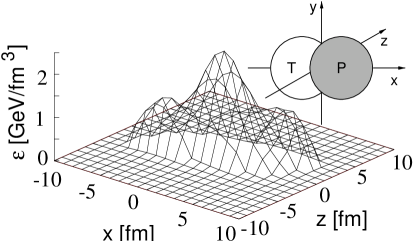
Figure 6: The initial condition of energy density distribution at $y=0$ fm in U+U 20 AGeV, sphere-sphere collision. In this case the impact parameter is 4.0 fm.

Figure 7: The initial condition of velocity distribution at $y=0$ fm in the same condition as fig. 7.

Figure 7 shows the energy density distribution of initial conditions in U+U 20 AGeV sphere-sphere collision at $b=4.0$ fm. From this figure we can see clearly the contribution from participant part and spectator part. For the initial velocity distribution we neglect the transverse flow because its value is small in the result of URASiMA. The initial flow distribution is given as,

$$v_{x}(x,y,z) = 0,$$

$$v_{y}(x,y,z) = 0,$$

$$v_{z}(x,y,z) = \frac{z}{t}B_{v}(x,y,z).$$ (85)

Here the distribution function $B_{v}(x,y,z)$ is given by,

$$B_{v}(x,y,z) = \frac{1}{c_{2}}[\exp(-\frac{(x-x_{cs})^{2}}{\sigma_{sx}^{2}}-\frac{(y-y_{cs})^{2}}{\sigma_{sy}^{2}}-\frac{(z-z_{cs})^{2}}{\sigma_{sz}^{2}})$$ (86)

$$+\exp(-\frac{(x+x_{cs})^{2}}{\sigma_{sx}^{2}}-\frac{(y+y_{cs})^{2}}{\sigma_{sy}^{2}}-\frac{(z+z_{cs})^{2}}{\sigma_{sz}^{2}})$$

$$+a_{2}\exp(-\frac{(x-x_{cp})^{2}}{\sigma_{px}^{2}}-\frac{(y-y_{cp})^{2}}{\sigma_{py}^{2}}-\frac{(z-z_{cp})^{2}}{\sigma_{pz}^{2}})],$$

where $c_{2}$ is normalization and $a_{2}$ is parameter and fixed to be 1.4. Figure 7 shows the initial velocity distribution in the same case as fig. 7. The flow in longitudinal direction is similar to Bjorken’s scaling solution in the central region.

3.3 Calculated Results

Figure 8: The time evolution of energy density of central region in U+U 20 AGeV with $b=0$ fm. The solid line, the dot-dashed line, and the dashed line stand for tip-tip collision, body-body collision, and sphere-sphere collision, respectively.

Figure 9: The time evolution of baryon number density distribution in the same case of fig. 9. The solid line, the dot-dashed line, and the dashed line stand for tip-tip collision, body-body collision, and sphere-sphere collision, respectively.

Figures 9 and 9 indicate the expansion of energy density and baryon number density in the central region. There is a slight difference in the life time in each case. The initial energy density and baryon density of body-body collision are the smallest among all three types of collisions and the difference between tip-tip collision and sphere-sphere collision is small. At initial time the difference of energy density among all three types of collision is $\Delta\epsilon\simeq 10\sim 20\%$ and the difference of time is $\Delta t\simeq 10\sim 20\%$ at $\epsilon=1$ GeV/fm³. However those kinds of difference among collision types do not appear at final time.

Figure 10: The behavior of $v_{2}$ as a function of the impact parameter in all cases. In this figure e10-b means that the incident energy is 10 AGeV in body-body collision and e10-s means that the incident energy is 10 AGeV in sphere-sphere collision and e20-t means that the incident energy is 20 AGeV in tip-tip collision and so on.

Figure 10 shows that behavior of $v_{2}$ of nucleon as a function of the impact parameter for each type of collision at 10 and 20 AGeV. The elliptic flow parameter, $v_{2}$, increases with impact parameter and reaches a peak at $b=3,4$ fm and decreases in every case. Furthermore for body-body collision $v_{2}$ does not vanish at $b=0$. Consequently, the effect of deformation is not negligible. In order to make this characteristic behavior clear we focus on the pressure distribution.

Figure 11 displays the pressure distribution in U+U 10 AGeV sphere-sphere collision. From the figures at $z\sim 0$ fm we can see that the pressure gradient in the $y$ direction increases with the impact parameter. Therefore one might consider that $v_{2}$ increases with impact parameter, because the velocity of produced particles in $x$ direction is larger than one in $y$ direction. But fig. 10 shows that the value of $v_{2}$ starts to decrease at about $b=3\sim 4$ fm. Here we focus on the pressure distribution in $z$-plane in fig. 11, and we can see that the effect of spectator increases with the impact parameter. Because the spectators block the flow in $x$ direction, the growth of flow in $x$ direction is suppressed. Consequently the behavior of $v_{2}$ is determined by both of the pressure gradient and the effect of spectator.

Figure 12 shows the pressure distribution at U+U 20 AGeV collision at $b=4.0$ fm. In $z$-plane there is a slight difference between tip-tip collision and sphere-sphere collision. On the other hand, in body-body collision the extension of the pressure distribution in $x$ direction is larger than in other cases. Therefore $v_{2}$ in body-body collision is less than one in sphere-sphere and tip-tip collision at any impact parameter.

Figure 13 shows the pressure distributions at U+U 10 AGeV and U+U 20 AGeV. Since there is a slight difference between U+U 10 AGeV and U+U 20 AGeV in the $z$-plane, the growth of $v_{2}$ in U+U 10 AGeV collision is similar to U+U 20 AGeV. In the $y$-plane the effect of spectator in U+U 20 AGeV is smaller than U+U 10 AGeV. Because the effect of Lorentz contraction becomes large in the large incident energy, the spectator becomes thin and the influence of it becomes small. Consequently the peak of $v_{2}$ moves to the large impact parameter at large incident energy.

Here, the value of $v_{2}$ which is influenced by deformation is about 0.015 from fig. 10. According to the analyses of the excitation function of the directed flow in ref. [21, 22], the flow becomes slow under phase transition, because the speed of sound becomes small in mixed phase, but the effect of the phase transition on flow is expected to be small in the AGS energy region. Therefore the effect of deformation is significant and the value of $v_{2}$ which is obtained in this section is important. Further detailed analysis on the relation between the effect of phase transition and deformation on flow may provide a new possible experimental probe of the phase transition.

$b$ = 0 fm

$b$ = 3 fm

$b$ = 8 fm

Figure 11: The impact parameter dependence of the pressure distribution in U+U 10 AGeV sphere-sphere collision at $t=20$ fm/$c$. The left part of figures displays the results at $z\sim 0$ fm and the right part of figures displays those at $y\sim 0$ fm. The highest values of the pressure distribution contour are 0.055 GeV/fm³ for $b=0$ fm, 0.05 GeV/fm³ for $b=3$ and 8 fm, respectively and the contour lines are drawn in steps of $\Delta p=$ 0.005 GeV/fm³.

tip-tip

sphere-sphere

body-body

Figure 12: The pressure distribution in tip-tip, sphere-sphere and body-body collision U+U 20 AGeV at $t=20$ fm/$c$. The impact parameter is 4 fm in all figures. The highest value of pressure distribution contour is 0.08 GeV/fm³ for all figures and the contour lines are drawn in steps of $\Delta p=$ 0.01 GeV/fm³.

$E$ = 10 AGeV

$E$ = 20 AGeV

Figure 13: The incident energy dependence of pressure distribution in U+U 10.0 AGeV and U+U 20.0 AGeV at $t=20$ fm/$c$. The highest value of the pressure distribution is 0.05 GeV/fm³ in 10.0 AGeV collision and 0.07 GeV/fm³ in 20.0 AGeV collision. The contour lines are drawn in steps $\Delta p=$ 0.005 GeV/fm³ in 10.0 AGeV collision and in steps $\Delta p=$ 0.01 GeV/fm³ in 20.0 AGeV collision.

4 Summary

We present (3+1)-dimensional relativistic hydrodynamical model of the Lagrangian hydrodynamics without assuming symmetrical conditions. Our algorithm is based on the entropy conservation law and the baryon number conservation law explicitly. In our algorithm we trace the volume elements of fluid along the stream of flux. By using our relativistic hydrodynamical model based on the Lagrangian hydrodynamics, the path of the each volume element in the phase diagram is able to be traced quite easily. Therefore we can investigate directly how the phase transition takes place and affects physical phenomenon in an ultra-relativistic nuclear collision.

Using this model, we have investigated the effect of anisotropic flow in deformed uranium collisions. The behavior of the flow depends on the pressure distribution and shadowing. Especially shadowing effect increases with the impact parameter. As for differences in collision types, there exists only a slight difference between tip-tip collision and sphere-sphere collision. On the other hand, $v_{2}$ in body-body collision is different from sphere-sphere collision, i.e. absolute value of $v_{2}$ is maximum at $b=0$ fm. In light of the effect of the incident energy on $v_{2}$, the peak of $v_{2}$ is shifted to large impact parameter region, because the shadowing effect decreases with increasing the incident energy. We accordingly conclude that body-body collision is promising for studying the nuclear equation of states and the property of QCD phase transition. These results are consistent with ref. [24].

We shall remark the following things: In actual experiment, U+U collision is the superposition of different types of collision like tip-tip, body-body and so on. Since the contribution of body-body collision is not negligible, $v_{2}$ does not equal to zero at $b=0$ fm. Furthermore, the shadowing has a large effect on $v_{2}$.

In this paper we have applied our relativistic hydrodynamical model to the anisotropic flow. Many kinds of applications of our relativistic hydrodynamical model can be considered. Using our hydrodynamical model, we can analyze directly the phenomena which are sensitive to the phase transition. For example, we can argue how the phase transition has effect to the minimum of the excitation function of the directed flow, discussing the trajectory of volume element of fluid in $T$-$\mu$ plane. Whether “nutcracker” phenomena can be observed in our Lagrangian hydrodynamical model is also interesting problem. Hanbury Brown-Twiss effect (HBT) and the influence of anisotropic flow to HBT can also be investigated.

Acknowledgment The authors would like to thank prof. Osamu Miyamura for his encouragement to pursue this project and fruitful discussions. They thank Dr. Nobuo Sasaki for providing URASiMA and useful comments. They are grateful to prof. Atsushi Nakamura for reading the manuscript carefully. Calculations have been done at the HSP system of the Institute for Nonlinear Sciences and Applied Mathematics, Hiroshima University. This work is supported by the Grant in Aide for Scientific Research of the Ministry of Education and Culture in Japan. (No. 11440080)

References

- [1] For example, see the proceedings of Quark Matter ’99, Nucl. Phys. A661, 3c (1999)
- [2] J. Barrette et al. : E877, Phys. Rev. C 56, 3254 (1997)
- [3] C. Pinkenburg et al. : E895, Phys. Rev. Lett. 83, 1295 (1999)
- [4] H. Appelshuser et al. : NA49, Phys. Rev. Lett. 80, 4136 (1998)
- [5] A. M. Poskanzer and S. A. Voloshin for NA49 Collaboration, Nucl. Phys. A661, 341c (1999)
- [6] M. M. Aggarwal et al. : WA98, nucl-ex/9807004
- [7] D. H. Rischke et al. , Nucl. Phys. A595, 346 (1995)
- [8] P. Danielewicz, Roy A. Lacey, P.-B. Gossiaux, C. Pinkenburg, P. Chung, J. M. Alexander, and R. L. McGrath, Phys. Rev. Lett. 81, 2438 (1998)
- [9] H. Sorge, Phys. Rev. Lett. 82, 2048 (1999)
- [10] J. D. Bjorken, Phys. Rev. D 27, 140 (1983)
- [11] Y. Akase, M. Mizutani, S. Muroya, and M. Yasuda, Prog. Theor. Phys. 85, 305 (1991); S. Muroya, H. Nakamura, and M. Namiki, Prog. Theor. Phys. Suppl. No.120, 209 (1995)
- [12] T. Ishii and S. Muroya, Phys. Rev. D 46, 5156 (1992)
- [13] J. Alam, S. Raha, and B. Sinha, Phys. Rep. 273, 243 (1996); J. Alam, D. K. Srivastava, B. Sinha, and D. N. Basu, Phys. Rev. D 48, 1117 (1993)
- [14] U. Ornik, M. Plmer, B. R. Schlei, D. Strottman, and R. M. Weiner, Phys. Rev. C 54, 1381 (1996)
- [15] J. Sollfrank, P. Huovinen, M. Kataja, P. V. Ruuskanen, M. Prakash, and R. Venugopalan, Phys. Rev. C 55, 392 (1997)
- [16] C. M. Hung and E. Shuryak, Phys. Rev. C 57, 1891 (1998)
- [17] B. R. Schlei and D. Strottman, Phys. Rev. C 59, R9 (1999)
- [18] K. Morita, S. Muroya, H. Nakamura, and C. Nonaka, Phys. Rev. C 61, 034904 (2000)
- [19] D. Teaney and E. V. Shuryak, Phys. Rev. Lett. 83, 4951 (1999)
- [20] P. F. Kolb, J. Sollfrank, and U. Heinz, Phys. Lett. B 459, 667 (1999); P. K. Kolb, J. Sollfrank, and U. Heinz, hep-ph/0006129
- [21] D. H. Rischke, Y. Prsn, J. A. Maruhn, H. Stcker, and W. Greiner, Heavy Ion Phys. 1, 309 (1995)
- [22] J. Brachmann, S. Soff, A. Dumitru, H. Stcker, J. A. Maruhn, and W. Greiner, Phys. Rev. C 61, 024909 (2000); J. Brachmann, A. Dumitru, H. Stcker, and W. Greiner, nucl-th/9912014
- [23] E. V. Shuryak, Phys. Rev. C 61, 034905 (2000)
- [24] Bao-An Li, Phy. Rev. C 61, 02193(R) (2000)
- [25] Ben-Hao Sa and An Tai, nucl-th/9912028
- [26] C. Nonaka, N. Sasaki, S. Muroya, and O. Miyamura, Nucl. Phys. A661, 353c (1999)
- [27] D. H. Rischke, M. I. Gorenstein, H. Stcker, and W. Greiner, Z. Phys. C 51 (1991) 485
- [28] Particle Data Group, Eur. Phys. J. C 3, 1 (1998)
- [29] L. D. Landau and E. M. Lifsitz, Fluid Mechanics, Pergamon Press., Oxford(1989)
- [30] M. Gyulassy, K. Kajantie, H. Kurki-Suonio, and L. Mclerran, Nucl. Phys. B237, 477 (1984)
- [31] S. Muroya and C. Nonaka, Bull. Tokuyama Women’s College 6, 45 (1999); nucl-th/9709004
- [32] A. Bohr and B. Mottelson, Nuclear Structure, Vol. II, P. 133 (Benjamin, New York, 1975)
- [33] S. Dat, K. Kumagai, O. Miyamura, H. Sumiyoshi, and X. Z. Zhang, J. Phys. Soc. Japan. 64, 766 (1995)
- [34] N. Sasaki and O. Miyamura, Prog. Theor. Phys. Suppl. 129, 39 (1997)
- [35] N. Sasaki, in preparation
- [36] F. Cooper and G. Frye, Phys. Rev. D 10, 186 (1974)
- [37] U. Heinz, Nucl. Phys. A638, 367c (1998)
- [38] Jean-Paul Blaizot and Jean-Yves Ollitraut, in Quark-Gluon Plasma, R. C. Hwa ed.(World Scientific, Singapole, 1990)
- [39] J. Ollitrault, Phys. Rev. D 46, 229 (1992); J. Ollitrault, Phys. Rev. D 48 1132 (1993)