July 2000
UM-P-029/2000
RCHEP-005/2000
 
Further studies on relic neutrino asymmetry generation I:
the adiabatic Boltzmann limit, non-adiabatic evolution,
and the classical harmonic oscillator analogue of the
quantum kinetic equations

Abstract

We demonstrate that the relic neutrino asymmetry evolution equation derived from the quantum kinetic equations (QKEs) reduces to the Boltzmann limit that is dependent only on the instantaneous neutrino distribution functions, in the adiabatic limit in conjunction with sufficient damping. An original physical and/or geometrical interpretation of the adiabatic approximation is given, which serves as a convenient visual aid to understanding the sharply contrasting resonance behaviours exhibited by the neutrino ensemble in opposing collision regimes. We also present a classical analogue for the evolution of the difference in the $\nu_{\alpha}$ and $\nu_{s}$ distribution functions which, in the Boltzmann limit, is akin to the behaviour of the generic reaction $A\rightleftharpoons B$ with equal forward and reverse reaction rate constants. A new characteristic quantity, the matter and collision-affected mixing angle of the neutrino ensemble, is identified here for the first time. The role of collisions is revealed to be twofold: (i) to wipe out the inherent oscillations, and (ii) to equilibrate the $\nu_{\alpha}$ and $\nu_{s}$ distribution functions in the long run. Studies on non-adiabatic evolution and its possible relation to rapid oscillations in lepton number generation also feature, with the introduction of an adiabaticity parameter for collision-affected oscillations.

I Introduction

The effects of decohering collisions and coherent flavour oscillations on a neutrino ensemble are collectively quantified by the quantum kinetic equations (QKEs) [1, 2] which, in recent years, have been frequently applied in the study of neutrino asymmetry (difference in neutrino and antineutrino number densities) evolution in the early universe, with appreciable success [3, 4, 5]. In essence, the simplest scenario involves independent oscillations of an active neutrino $\nu_{\alpha}$ and its antineutrino $\overline{\nu}_{\alpha}$, commencing with equal number densities, to a corresponding, initially absent light sterile species, $\nu_{s}$ and $\overline{\nu}_{s}$, in an environment that alters the two sets of oscillation parameters in dissimilar ways. Both $\nu_{\alpha}\leftrightarrow\nu_{s}$ and $\overline{\nu}_{\alpha}\leftrightarrow\overline{\nu}_{s}$ systems evolve subject simultaneously to a biased collision scheme which, in crude terms, is blind to the sterile variety. For the appropriate vacuum oscillation parameters, numerical solutions to the exact QKEs demonstrate the combined effect to be one that sees the relic $\alpha$-neutrino asymmetry grow to orders of magnitude above the baryon–antibaryon asymmetry [3, 4, 5, 6]. For other relevant works see Ref. [7].

As much as one would like to use the QKEs directly in all applications, obtaining exact numerical solutions remains a computationally intensive task, given the necessity to track neutrinos at all momenta where nonzero feedback couples their development. Several approximate treatments have been employed in the past which, besides lifting the burden on the computer considerably, also on occasion offer valuable analytical insights on the nature of the asymmetry evolution [3, 6, 10]. Two such schemes are the well-established static approximation [3, 6], and the closely related adiabatic limit approximation introduced in Ref. [10].

Beginning with the QKEs, the adiabatic limit approach comprises a set of systematic approximations, leading ultimately to an approximate expression for the neutrino asymmetry evolution. The extraction procedure, however, was hitherto largely motivated by mathematical convenience; physical, or at least geometrical, interpretations of the intermediate steps and quantities that arose therein were lacking. It is thus our intention in this paper to examine the derivation of the adiabatic approximation more closely, and to assign definite physical meanings to as many mathematical manœuvres as possible. These new interpretations are most useful for visually tracking the evolution of the neutrino ensemble across a Mikheyev–Smirnov–Wolfenstein (MSW) resonance [11] in different collision regimes, and in understanding the nature of non-adiabatic evolution. We shall also demonstrate again, this time more assertively, that the adiabatic procedure leads to the elimination of phase dependence in the regime of interest: the approximate evolution equations for the neutrino distribution functions depend only on the distribution functions themselves, and not on the coherence history of the ensemble. In other words, the QKEs yield classical-like Boltzmann equations in the adiabatic limit.

Our second goal in the present work is to draw attention to the similarity between some aspects of the QKEs and the behaviours of the more familiar classical linear harmonic oscillator. In particular, the evolution of the difference between the $\nu_{\alpha}$ and $\nu_{s}$ distribution functions in the adiabatic limit may be modelled by a damped harmonic oscillator with a decaying oscillation midpoint. This analogy turns out to be a very illuminating one that illustrates clearly the reason behind the remarkable accuracy and the conceptual correctness of the original heuristic static approximation. A new quantity, the neutrino ensemble’s matter and collision-affected mixing angle, is also established in the course.

Before proceeding, let us state plainly what we hope to achieve ultimately from these abstract analyses: Acquisition of a clear understanding of the physical processes that constitute the various computationally convenient approximations will leave us better equipped to improve on them. To this end, classical analogies are especially useful as visual aids. On a grander scale, studies of the QKEs per se may stand to benefit areas beyond relic neutrino asymmetry evolution, most notably transitions in multi-level atomic systems which are described by similar equations [12].

The structure of this paper is as follows: The exact QKEs are presented in Sec. II for the purpose of introducing the nomenclature. Section III is devoted to the discussion of the formal adiabatic procedure, in which we shall also present results from numerically integrating the pertinent approximate neutrino asymmetry evolution equation for the first time. The classical harmonic oscillator analogy is to be treated in Sec. IV, while Sec. V deals with the issue of non-adiabaticity and its possible relation to rapid oscillations in the asymmetry evolution. We conclude in Sec. VI.

II Neutrino asymmetry evolution and the quantum kinetic equations: nomenclature

We shall consider a two-flavour system consisting of an active species $\nu_{\alpha}$ (where $\alpha=e$, $\mu$ or $\tau$), and a sterile species $\nu_{s}$, where their respective abundances and the ensemble’s coherence status at momentum $p$ are encoded in the density matrices [1, 2]

$$\rho(p)=\frac{1}{2}[P_{0}(p)+{\bf P}(p)\cdot\sigma].$$ (1)

The vector ${\bf P}(p)=P_{x}(p)\hat{x}+P_{y}(p)\hat{y}+P_{z}(p)\hat{z}$ may be interpreted as the “polarisation” and $\sigma=\sigma_{x}\hat{x}+\sigma_{y}\hat{y}+\sigma_{z}\hat{z}$ are the Pauli matrices. In this notation, the $\nu_{\alpha}$ and $\nu_{s}$ distribution functions at $p$ are respectively

$$N_{\alpha}(p) = \frac{1}{2}[P_{0}(p)+P_{z}(p)]N^{\text{eq}}(p,0),$$ (2)

$$N_{s}(p) = \frac{1}{2}[P_{0}(p)-P_{z}(p)]N^{\text{eq}}(p,0),$$ (3)

for which we have chosen the reference distribution function $N^{\text{eq}}(p,0)$ to be of Fermi–Dirac (equilibrium) form,

$$N^{\text{eq}}(p,\mu)=\frac{1}{2\pi^{2}}\frac{p^{2}}{1+\exp\left(\frac{p-\mu}{T}\right)},$$ (4)

with chemical potential $\mu$ set to zero at temperature $T$. The four variables $P_{0}(p)$ and ${\bf P}(p)$ advance in time according to the quantum kinetic equations (QKEs)

$$\frac{\partial{\bf P}}{\partial t} = {\bf V}(p)\times{\bf P}(p)-D(p)[P_{x}(p)\hat{x}+P_{y}(p)\hat{y}]+\frac{\partial P_{0}}{\partial t}\hat{z},$$ (5)

$$\frac{\partial P_{0}}{\partial t} \simeq \Gamma(p)\left\{\frac{N^{\text{eq}}(p,\mu)}{N^{\text{eq}}(p,0)}-\frac{1}{2}[P_{0}(p)+P_{z}(p)]\right\},$$ (6)

where the quantities $D(p)=\Gamma(p)/2$ and ${\bf V}(p)$ individually characterise the collision-induced decohering and the matter-affected coherent aspects of the ensemble’s evolution respectively. Their approximate forms shall be detailed shortly. Note that the $\frac{\partial P_{0}}{\partial t}$ equation is not exact because the right hand side assumes thermal equilibrium for all species in the background plasma, while the $\nu_{\alpha}$ distribution is taken to be approximately thermal [10]. The properties of the antineutrino ensemble may be parameterised in a similar manner and subject to the same QKEs with the appropriate decoherence function and matter potential. Henceforth, all quantities pertaining to the $\overline{\nu}_{\alpha}\leftrightarrow\overline{\nu}_{s}$ system shall bear an overhead bar.

The vector ${\bf V}(p)$ reads [13]

$${\bf V}(p)=\beta(p)\hat{x}+\lambda(p)\hat{z},$$ (7)

with

$$\beta(p) = \frac{\Delta m^{2}}{2p}\sin 2\theta_{0},$$ (8)

$$\lambda(p) = \frac{\Delta m^{2}}{2p}[b(p)-a(p)-\cos 2\theta_{0}],$$ (9)

in which $\Delta m^{2}$ is the mass-squared difference between the neutrino states, $\theta_{0}$ is the vacuum mixing angle, and

$$a(p) = -\frac{4\zeta(3)\sqrt{2}G_{F}L^{(\alpha)}T^{3}p}{\pi^{2}\Delta m^{2}},$$ (10)

$$b(p) = -\frac{4\zeta(3)\sqrt{2}G_{F}A_{\alpha}T^{4}p^{2}}{\pi^{2}\Delta m^{2}m^{2}_{W}},$$ (11)

given that $G_{F}$ is the Fermi constant, $m_{W}$ the $W$-boson mass, $\zeta$ the Riemann zeta function and $A_{e}\simeq 17$, $A_{\mu,\,\tau}\simeq 4.9$. The quantity

$$L^{(\alpha)}=L_{\alpha}+L_{e}+L_{\mu}+L_{\tau}+\eta\equiv 2L_{\alpha}+\tilde{L},$$ (12)

combines the various asymmetries individually defined as

$$L_{\alpha}=\frac{n_{\alpha}-\overline{n}_{\alpha}}{n_{\gamma}},$$ (13)

where $n_{\alpha}=\int N_{\alpha}(p)dp$, $n_{\gamma}$ is the photon number density, and $\eta$ is a small term related to the cosmological baryon–antibaryon asymmetry. The authors of Ref. [4] have called $L^{(\alpha)}$ the effective total lepton number (for the $\alpha$-neutrino species), a name we shall also adopt. The condition $\lambda=0$ is identified with a Mikheyev–Smirnov–Wolfenstein (MSW) resonance [11].

The function $D(p)$ is equivalent to half of the total collision rate for $\nu_{\alpha}$ with momentum $p$, that is [1, 10],

$$D(p)=\frac{1}{2}\Gamma(p)=\frac{1}{2}\frac{p}{\langle p\rangle_{0}}[y_{\alpha}G^{2}_{F}T^{5}(1-z_{\alpha}L_{\alpha})+{\cal O}(L^{2}_{\alpha})],$$ (14)

where $\langle p\rangle_{0}\simeq 3.15T$ is the average momentum for a relativistic Fermi–Dirac distribution with zero chemical potential, $y_{e}\simeq 4$, $y_{\mu,\,\tau}\simeq 2.9$ and $z_{e}\simeq 0.1$, $z_{\mu,\,\tau}\simeq 0.04$.

The corresponding functions $\overline{\bf V}(p)$ and $\overline{D}(p)$ for the antineutrino system are obtained from their ordinary counterparts by replacing $L^{(\alpha)}$ and $L_{\alpha}$ with $-L^{(\alpha)}$ and $-L_{\alpha}$ in Eqs. (10) and (14) respectively.

We conclude this section by noting that a direct time evolution equation for the neutrino asymmetry may be derived from the QKEs together with $\alpha+s$ lepton number conservation [10], which reads

$$\frac{dL_{\alpha}}{dt}=\frac{1}{2n_{\gamma}}\int\beta[P_{y}(p)-\overline{P}_{y}(p)]N^{\text{eq}}(p,0)dp.$$ (15)

As well as serving as the backbone on which to develop useful approximations, this expression is useful when numerically solving the QKEs. Although it is redundant, Eq. (15) has the virtue of tracking the crucial quantity $L_{\alpha}$ without the need to take the difference of two large numbers.

III Adiabatic limit

A The Boltzmann limit

The adiabatic limit approximation introduced in of Ref. [10] consists of firstly setting the repopulation function in Eq. (5) to zero, i.e., $\frac{\partial P_{0}}{\partial t}\simeq 0$, such that the QKEs simplify to the homogeneous equations

$$\frac{\partial}{\partial t}\left(\begin{array}[]{c}P_{x}\\ P_{y}\\ P_{z}\end{array}\right)\simeq\left(\begin{array}[]{ccc}-D&-\lambda&0\\ \lambda&-D&-\beta\\ 0&\beta&0\end{array}\right)\left(\begin{array}[]{c}P_{x}\\ P_{y}\\ P_{z}\end{array}\right)\equiv{\cal K}{\bf P},$$ (16)

where the dependent variables and coefficients are understood to be functions of both time and momentum.

We solve Eq. (16) by establishing a parameter-dependent “instantaneous diagonal basis” ${\cal S}_{q}\equiv{\cal S}_{q}(D,\,\lambda,\,\beta)=(\begin{array}[]{ccc}\hat{q}_{1},&\hat{q}_{2},&\hat{q}_{3}\end{array})$, onto which we map the vector ${\bf P}$ from its original “fixed” coordinate system ${\cal S}=(\begin{array}[]{ccc}\hat{x},&\hat{y},&\hat{z}\end{array})$ via

$$\left(\begin{array}[]{c}Q_{1}\\ Q_{2}\\ Q_{3}\end{array}\right)\equiv{\bf Q}={\cal U}{\bf P}.$$ (17)

The transformation matrix ${\cal U}$ and its inverse ${\cal U}^{-1}$ diagonalise the matrix ${\cal K}$ in Eq. (16) by definition,

$${\cal K}_{d}\equiv\text{diag}(k_{1},\,k_{2},\,k_{3})={\cal UKU}^{-1},$$ (18)

where the eigenvalues $k_{1}$, $k_{2}$ and $k_{3}$ are roots of the cubic characteristic equation

$$k^{3}+2Dk^{2}+(D^{2}+\lambda^{2}+\beta^{2})k+\beta^{2}D=0,$$ (19)

the discriminant of which is identically

$$\Delta=4\beta^{6}-\beta^{4}D^{2}+12\beta^{4}\lambda^{2}-20\beta^{2}D^{2}\lambda^{2}+4D^{4}\lambda^{2}+12\beta^{2}\lambda^{4}+8D^{2}\lambda^{4}+4\lambda^{6}.$$ (20)

Under most circumstances (for example, the individual cases of $|\lambda|\gg D$ and $|\beta|\gg D$), the inequality $\Delta>0$ holds such that two of the three eigenvalues occur predominantly as a complex conjugate pair, which may be conveniently parameterised as

$$k_{1,\,2}=-d\pm i\omega,$$ (21)

where $d$ and $\omega$, both real and positive, are readily interpreted as the effective damping factor and effective oscillation frequency respectively. These phenomenological parameters arise since the QKEs couple the damped and oscillatory aspects of the time evolution, and are to be compared with what could be called the bare damping factor $D$ and the bare matter-affected oscillation frequency $\Omega\equiv\sqrt{\beta^{2}+\lambda^{2}}$. The remaining root $k_{3}$ of Eq. (19) is real and negative, and bears several simple but elucidating relationships to $k_{1}$ and $k_{2}$,

$$k_{3} = -\frac{\beta^{2}D}{d^{2}+\omega^{2}},$$ (22)

$$d = D+\frac{k_{3}}{2},$$ (23)

$$\omega^{2} = \lambda^{2}+\beta^{2}+k_{3}D+\frac{3}{4}k_{3}^{2},$$ (24)

to be further discussed in Section IV. These equations show that $k_{3}$ quantifies the “misalignment” between the effective and bare damping factor, and between the effective and bare oscillation frequency.

The only (so far) unambiguously identified instance for which the discriminant is zero or negative ($\Delta\leq 0$) occurs when the conditions $D\gg|\beta|$ and $\lambda^{2}\stackrel{{\scriptstyle<}}{{\sim}}\frac{\beta^{4}}{4D^{2}}$ are simultaneously satisfied, in which case all eigenvalues are real and generally distinct with the exception of $\Delta=0$, where at least two roots are equal. The interested reader is referred to Appendix A for the mathematical details. For clarity, we shall deal exclusively with off-resonance evolution in this subsection, which translates loosely into requiring $|\lambda|>D,\,|\beta|$, so as to ensure the existence of complex conjugate eigenvalues. The study of resonance behaviour i.e., where $\lambda\simeq 0$, is deferred to Sec. III B.

For $\lambda\neq 0$, the matrix ${\cal U}^{-1}$ consists of the normalised eigenvectors

$$\kappa_{i}=\frac{1}{{\cal N}_{i}}\left(\begin{array}[]{c}1\\ -\frac{D+k_{i}}{\lambda}\\ -\beta\frac{D+k_{i}}{\lambda k_{i}}\end{array}\right),$$ (25)

in the columns, while the row vectors

$$v_{i}=-{\cal N}_{i}k_{i}\left(\frac{1}{D}\prod_{j\neq i}\frac{D+k_{j}}{k_{i}-k_{j}},\quad\lambda\prod_{j\neq i}\frac{1}{k_{i}-k_{j}},\quad\frac{\lambda}{\beta D}\prod_{j\neq i}\frac{k_{j}}{k_{i}-k_{j}}\right),$$ (26)

constitute the inverse matrix ${\cal U}$, with the $i$th normalisation factor given by

$${\cal N}_{i}=\frac{1}{|\lambda k_{i}|}\sqrt{\lambda^{2}|k_{i}|^{2}+(\beta^{2}+|k_{i}|^{2})|D+k_{i}|^{2}},$$ (27)

or explicitly, with the aid of Eqs. (22) to (24),

$${\cal N}_{1} = {\cal N}_{2}=\frac{1}{|\lambda|}\sqrt{2[\lambda^{2}+\beta^{2}+k_{3}(D+k_{3})]},$$ (28)

$${\cal N}_{3} = \frac{\beta}{|\lambda k_{3}|}\sqrt{D(D+k_{3})}.$$ (29)

In this new basis ${\cal S}_{q}$, the unit vector $\hat{q}_{3}$ represents the axis about which ${\bf P}$ precesses. This precession axis coincides, by definition, with the matter potential vector ${\bf V}$ in the absence of collisions (i.e., $D=0$), residing entirely on the $xz$-plane when viewed in the fixed coordinate system ${\cal S}$. Otherwise the alignment is inexact in the general case, where a nonzero D generically endows $\hat{q}_{3}$ with a small $y$-component evident in the transformation matrix ${\cal U}^{-1}$ in Eq. (25), that is,

$$\hat{q}_{3}={\cal U}^{-1}_{x3}\hat{x}+{\cal U}^{-1}_{y3}\hat{y}+{\cal U}^{-1}_{z3}\hat{z},$$ (30)

where

$$\left|{\cal U}^{-1}_{x3}\right|^{2} = \frac{\beta^{2}}{(D+k_{3})^{2}+\lambda^{2}+\beta^{2}}\left[1-\frac{D(D+k_{3})}{(D+k_{3})^{2}+\lambda^{2}+\beta^{2}}\right]\stackrel{{\scriptstyle D=0}}{{\longrightarrow}}\frac{\beta^{2}}{\lambda^{2}+\beta^{2}},\$$ (31)

$$\left|{\cal U}_{y3}^{-1}\right|^{2} = \frac{\beta^{2}D(D+k_{3})}{\left[(D+k_{3})^{2}+\lambda^{2}+\beta^{2}\right]^{2}}\stackrel{{\scriptstyle D=0}}{{\longrightarrow}}0,$$ (32)

$$\left|{\cal U}^{-1}_{z3}\right|^{2} = \frac{(D+k_{3})^{2}+\lambda^{2}}{(D+k_{3})^{2}+\lambda^{2}+\beta^{2}}\stackrel{{\scriptstyle D=0}}{{\longrightarrow}}\frac{\lambda^{2}}{\lambda^{2}+\beta^{2}}.$$ (33)

The $D=0$ (i.e., $\hat{q}_{3}\parallel{\bf V}$) limit of Eq. (31) is to be compared with Eq. (7). The variables $Q_{1}$ and $Q_{2}$ quantify the actual precession in conjunction with their associating complex vectors, $\hat{q}_{1}$ and $\hat{q}_{2}$, that sweep the plane perpendicular to $\hat{q}_{3}$. Figure 8 shows schematically the relationship between the ${\cal S}$ and ${\cal S}_{q}$ bases.

Rewriting Eq. (16) in the new instantaneous ${\cal S}_{q}$ basis, we obtain

$$\frac{\partial{\bf Q}}{\partial t}={\cal K}_{d}{\bf Q}-{\cal U}\frac{\partial{\cal U}}{\partial t}^{-1}{\bf Q},$$ (34)

where the $3\times 3$ matrix ${\cal U}\frac{\partial{\cal U}}{\partial t}^{-1}$ exemplifies the system’s explicit dependence on $\frac{\partial D}{\partial t}$, $\frac{\partial\lambda}{\partial t}$ and $\frac{\partial\beta}{\partial t}$, and in general contains nonzero off-diagonal entries. Under certain circumstances, these time derivatives are inconsequentially small relative to terms in the diagonal matrix ${\cal K}_{d}$ (see Ref. [10] for the relevant constraints). When these bounds hold, we are entitled to take the adiabatic limit, defined by ${\cal U}\frac{\partial{\cal U}}{\partial t}^{-1}\simeq 0$, or equivalently,

$${\cal U}(D+\delta D,\,\lambda+\delta\lambda,\,\beta+\delta\beta){\cal U}^{-1}(D,\,\lambda,\,\beta)\simeq\text{diag}(1,1,1),$$ (35)

such that the basis ${\cal S}_{q}(D,\,\lambda,\,\beta)$ maps directly onto the neighbouring ${\cal S}_{q}(D+\delta D,\,\lambda+\delta\lambda,\,\beta+\delta\beta)$ as the parameters $D$, $\lambda$ and $\beta$ slowly vary with time.

The formal solution to the now completely decoupled system of differential equations for ${\bf Q}$ is simply

$${\bf Q}(t)\simeq\text{diag}\left(e^{\int^{t}_{0}k_{1}(t^{\prime})dt^{\prime}},\;e^{\int^{t}_{0}k_{2}(t^{\prime})dt^{\prime}},\;e^{\int^{t}_{0}k_{3}(t^{\prime})dt^{\prime}}\right){\bf Q}(0),$$ (36)

and consequently,

$${\bf P}(t)\simeq{\cal U}^{-1}(t)\text{diag}\left(e^{\int^{t}_{0}k_{1}(t^{\prime})dt^{\prime}},\;e^{\int^{t}_{0}k_{2}(t^{\prime})dt^{\prime}},\;e^{\int^{t}_{0}k_{3}(t^{\prime})dt^{\prime}}\right){\cal U}(0){\bf P}(0).$$ (37)

Note that this solution is “formal” because the eigenvalues $k_{i}$ depend on the asymmetry $L_{\alpha}$, and hence on $P_{z}$, through the function $\lambda$.

At this point, we alert the reader to a mathematical subtlety. Equations (36) and therefore (37) are in fact poorly defined if the time integration encompasses regions where two or more eigenvalues are identical. In this case, the matrix ${\cal K}$ has momentarily less than three distinct eigenvectors, thereby rendering the transformation matrix ${\cal U}^{-1}$ uninvertible. Fortunately, such instances, besides their rarity (see Appendix A), have virtually no bearings on the outcome as we shall see in due course.

From Eq. (37), we extract a formal expression for $P_{y}(t)$ in terms of $P_{z}(t)$,

$$P_{y}(t)\simeq\frac{{\cal U}^{-1}_{y1}(t)e^{\int^{t}_{0}k_{1}(t^{\prime})dt^{\prime}}Q_{1}(0)+{\cal U}^{-1}_{y2}(t)e^{\int^{t}_{0}k_{2}(t^{\prime})dt^{\prime}}Q_{2}(0)+{\cal U}^{-1}_{y3}(t)e^{\int^{t}_{0}k_{3}(t^{\prime})dt^{\prime}}Q_{3}(0)}{{\cal U}^{-1}_{z1}(t)e^{\int^{t}_{0}k_{1}(t^{\prime})dt^{\prime}}Q_{1}(0)+{\cal U}^{-1}_{z2}(t)e^{\int^{t}_{0}k_{2}(t^{\prime})dt^{\prime}}Q_{2}(0)+{\cal U}^{-1}_{z3}(t)e^{\int^{t}_{0}k_{3}(t^{\prime})dt^{\prime}}Q_{3}(0)}P_{z}(t).$$ (38)

Recall from Eq. (21) that the eigenvalues $k_{1}$ and $k_{2}$ are prevailingly composites of a real damping factor $d$ and an imaginary oscillatory component $\omega$. Given an ample $\lambda$ such that the effective oscillation frequency reads $\omega^{2}\simeq\lambda^{2}$ in Eq. (24), the real eigenvalue $k_{3}$ is guaranteed to be small according to Eq. (22), while the phenomenological damping becomes $d\simeq D$ by Eq. (23). Since $k_{3}$ scales with $D$, a comparatively large $d$ will always quickly reduce the corresponding exponentials in Eq. (38) to zero relative to the “decay” time of their $k_{3}$ counterpart, wiping out the accompanying rapid oscillations in the process. The condition $D\gg|\beta|$ is a bonus which contributes to accomplishing the said exponential damping at an even faster rate over the time scale of the $k_{3}$ decay. Installing the collision dominance approximation

$$e^{\int^{t}_{0}k_{1,\,2}(t^{\prime})dt^{\prime}}\to 0,$$ (39)

in Eq. (38), we obtain

$$P_{y}(t)\simeq\frac{{\cal U}_{y3}^{-1}(t)}{{\cal U}_{z3}^{-1}(t)}P_{z}(t)=\frac{k_{3}}{\beta}P_{z}(t),$$ (40)

which, together with its antineutrino analogue, allows us to express the neutrino asymmetry evolution equation in Eq. (15) in an approximate form,

$$\frac{dL_{\alpha}}{dt}\simeq\frac{1}{2n_{\gamma}}\int\left\{k_{3}[N_{\alpha}(p)-N_{s}(p)]-\overline{k}_{3}[\overline{N}_{\alpha}(p)-\overline{N}_{s}(p)]\right\}dp.$$ (41)

Observe that Eq. (41) involves only the $\nu_{\alpha}$ and $\nu_{s}$ distribution functions at any given time. Interestingly, phase dependence has been eliminated by the adiabatic procedure in conjunction with appreciable damping (collision dominance); the coherence status of the neutrino ensemble has minimal influence the asymmetry’s time evolution. Geometrically, the quantity $P_{y}(t)/P_{z}(t)$ in Eq. (40) is but the instantaneous ratio of the $y$- and $z$-components of the axis $\hat{q}_{3}$ in the limit of zero-amplitude precession. We shall henceforth refer to this condition as the Boltzmann limit of the QKEs. Note also that Eq. (41) has the form of a classical-style rate equation [see Eq. (72) below] with the neutrino and antineutrino transition rates computed to be $|k_{3}|/2$ and $|\overline{k}_{3}|/2$ respectively.

For computational purposes, an auxiliary expression describing sterile neutrino production for each momentum state $p$ may be obtained similarly in the Boltzmann limit [10],

$$\frac{d}{dt}\left[\frac{N_{s}(p)}{N^{\text{eq}}(p,0)}\right]=-\frac{1}{2}\beta P_{y}(p)\simeq-\frac{k_{3}}{2}\left[\frac{N_{\alpha}(p)-N_{s}(p)}{N^{\text{eq}}(p,0)}\right],$$ (42)

to be employed in tracking the quantity $N_{s}(p)$ in Eq. (41). The $\nu_{\alpha}$ distribution function in the same equation is approximated to be

$$N_{\alpha}(p)\simeq N^{\text{eq}}(p,\mu),$$ (43)

with the interpretation that the neutrino momentum state $p$ is instantaneously repopulated. Thus Eqs. (41) to (43) form a fully serviceable set to be simultaneously solved to give $L_{\alpha}$ as a function of time.

B Resonance behaviour: the $\lambda\simeq 0$ case

Reference [10] did not provide a full analysis of collision-affected adiabatic evolution through an MSW resonance. Since resonance behaviour is a very important issue in the study of lepton asymmetry growth, we now provide a careful treatment of this topic.

As an incentive to study the vicinity of an MSW resonance, let us observe the solutions $k$ to the characteristic equation, Eq. (19), at exactly $\lambda=0$,

$$\left.k\right|_{\lambda=0}=-D,\quad-\frac{D}{2}\pm\frac{\sqrt{D^{2}-4\beta^{2}}}{2}.$$ (44)

Evidently, whether the square root evaluates to an imaginary or a real number is conditional to the relative sizes of the arguments $D$ and $\beta$. If the former ensues, we are forced to identify the root $-D$ with the real eigenvalue $k_{3}$ which is now twice the magnitude of the effective damping factor $d=D/2$ such that the off-resonance “damping versus decay” rationale of Sec. III A no longer applies. The latter scenario is, contrary to off-resonance behaviour, non-oscillatory, and requires a new interpretation.

1 Case 1: $|\beta|\stackrel{{\scriptstyle>}}{{\sim}}D$

There are two distinct situations covered under this heading. The first is where adiabatic and collision dominated evolution occurs on either side of the resonance, with the condition $|\beta|\stackrel{{\scriptstyle>}}{{\sim}}D$ maintained during the crossing. This amounts to requiring that

$$\sin^{2}2\theta \stackrel{{\scriptstyle>}}{{\sim}} 3.6\times 10^{-24}y_{\alpha}^{2}\frac{|\Delta m^{2}|y}{L^{(\alpha)3}}$$ (45)

$$\sim 10^{-7},$$ (46)

where $y=p/T$ is a dimensionless quantity not to be confused with $y_{\alpha}$, and we have used Eqs. (8) and (14) evaluated at resonance, $\cos 2\theta-a(p)\simeq 0$. The last approximate inequality in Eq. (45) is established by setting $y\simeq 3.15$ (i.e., average momentum), $|\Delta m^{2}|\sim 1\,\text{eV}^{2}$, and $L^{(\alpha)}\sim 10^{-5}$ is a typical value for the asymmetry immediately after exponential growth.

The second scenario is where $D$ is genuinely small enough so that the collision dominance approximation cannot be made even outside of the resonance region. This situation typically obtains, independently of the vacuum oscillation parameters, at lower temperatures since $D$ decreases with temperature as $T^{5}$ according to Eq. (14).

It is easy to convince oneself by inspecting the discriminant in Eq. (20) that a dominating $\beta$ ensures the existence of complex eigenvalues, and thereby preserves the precessive nature of the evolution of the polarisation vector ${\bf P}$ for all $\lambda$. At $\lambda=0$, the solutions to the characteristic equation, Eq. (19), are

$$\left.k_{1,\,2}\right|_{\lambda=0,\,|\beta|\stackrel{{\scriptstyle>}}{{\sim}}D} = -\frac{D}{2}\pm i\frac{\sqrt{4\beta^{2}-D^{2}}}{2},$$ (47)

$$\left.k_{3}\right|_{\lambda=0,\,|\beta|\stackrel{{\scriptstyle>}}{{\sim}}D} = -D,$$ (48)

where the sole real root is always identified as $k_{3}$, which, as mentioned earlier, is clearly larger than the real components of $k_{1}$ and $k_{2}$, i.e., the effective damping factor $d=D/2$. The corresponding transformation matrices evaluate to

$$\left.{\cal U}^{-1}\right|_{\lambda=0,\,|\beta|\stackrel{{\scriptstyle>}}{{\sim}}D} = \left(\begin{array}[]{ccc}0&0&1\\ -\frac{1}{\sqrt{2}}\frac{k_{1}}{\beta}&-\frac{1}{\sqrt{2}}\frac{k_{2}}{\beta}&0\\ -\frac{1}{\sqrt{2}}&-\frac{1}{\sqrt{2}}&0\end{array}\right),$$ (52)

$$\left.{\cal U}\right|_{\lambda=0,\,|\beta|\stackrel{{\scriptstyle>}}{{\sim}}D} = \left(\begin{array}[]{ccc}0&i\beta\sqrt{\frac{2}{4\beta^{2}-D^{2}}}&-ik_{2}\sqrt{\frac{2}{4\beta^{2}-D^{2}}}\\ 0&-i\beta\sqrt{\frac{2}{4\beta^{2}-D^{2}}}&ik_{1}\sqrt{\frac{2}{4\beta^{2}-D^{2}}}\\ 1&0&0\end{array}\right),$$ (56)

where the precession axis $\hat{q}_{3}$ now lies in the $x$-direction, and the vectors $\hat{q}_{1}$ and $\hat{q}_{2}$ trace out accordingly a surface roughly parallel to the $yz$-plane.

Let us now track the evolution of ${\bf P}$, as depicted in Fig. 8, for the situation where collision dominance holds on either side of the resonance crossing. As the matter potential vector ${\bf V}$, initially at $(+\beta,\,0,\,+\lambda)$, is rotated on the $xz$-plane and decoherence function $D$ independently modified, the instantaneous unit vector $\hat{q}_{3}$ moves through a continuum of predefined positions in the $(+x,\,-y,\,+z)$ block dictated by the transformation matrix ${\cal U}^{-1}$, while ${\bf P}$ precesses about it. The vector $\hat{q}_{3}$ gradually aligns with the $x$-axis as we approach $\lambda=0$, such that the decay of $Q_{3}$ becomes increasingly dependent on the parameters that govern the evolution of $P_{x}$. This is manifested in the escalating magnitude of the eigenvalue $k_{3}$, which reaches a zenith of $|-D|$ when $\hat{q}_{3}$ and $\hat{x}$ are completely parallel at $\lambda=0$ by Eqs. (47) and (52), and $Q_{3}$ and $P_{x}$ are momentarily equivalent. Meanwhile, the two variables of interest, $P_{y}$ and $P_{z}$, become progressively more oscillatory as we cross the resonance region for the following reason.

In the adiabatic limit, the precessive behaviour of ${\bf P}$ is parameterised by the complex conjugate variables $Q_{1}$ and $Q_{2}$, and driven by the imaginary component of the corresponding eigenvalues $k_{1}$ and $k_{2}$. The magnitudes of the oscillatory components in $P_{x,y,z}$ are therefore dependent on two factors: (i) exponential damping of $Q_{1}$ and $Q_{2}$ through the real part of $k_{1}$ and $k_{2}$, and (ii) the “intrinsic” oscillation amplitudes prescribed by the transformation matrix ${\cal U}^{-1}$, or equivalently, the projections of the instantaneous eigenvectors $\hat{q_{1}}$ and $\hat{q_{2}}$ onto the fixed ${\cal S}$ basis. For the $|\beta|\stackrel{{\scriptstyle>}}{{\sim}}D$ case, Eq. (47) shows that the effective damping factor $d$ in $k_{1}$ and $k_{2}$ diminishes from $\sim D$ to an all-time low of $D/2$. This means that the variables $Q_{1}$ and $Q_{2}$ are no longer preferentially exponentially damped relative to the decay of $Q_{3}$ which now occurs at a comparable rate $\sim D$. On this account alone, no single term in Eq. (38) stands out as the presiding factor in the resonance region. At the same time, the evolution of $P_{y}$ and $P_{z}$ is now almost totally described by $Q_{1}$ and $Q_{2}$, because of a growing alignment between the $q_{1}q_{2}$- and $yz$-planes. Complete alignment (and therefore purely oscillatory behaviour in $P_{y}$ and $P_{z}$) is attained at exactly $\lambda=0$ as shown in Eq. (52).

On the other side of the resonance, $\hat{q}_{3}$ resides in the $(+x,\,+y,\,-z)$ block while ${\bf V}=(+\beta,\,0,-\lambda)$ continues to move down the $xz$-plane (see Fig. 8). The variable $Q_{3}$ regains control as $|\lambda|$ increases, and the system advances in time as discussed in Sec. III A.

The oscillatory terms at resonance play a pivotal role in partially propelling the asymmetry growth through the MSW effect (dominant mode for $|\beta|\gg D$, i.e., negligible collision rate). In fact, in regimes where collisions are completely absent (i.e., $D=0$), one may recover from the approximate solution to the QKEs in Eq. (37) the common expression for the adiabatic MSW survival probability [10]. Geometrically, adiabatic $|\beta|\stackrel{{\scriptstyle>}}{{\sim}}D$ evolution carries the polarisation vector ${\bf P}$ from the $(+x,\,-y,\,+z)$ to the $(+x,\,+y,\,-z)$ block across an MSW resonance following the precession axis $\hat{q}_{3}$. But as far as Eq. (41) is concerned, coherent MSW transitions are evidently dependent on the history of the neutrino ensemble, and therefore outside the Boltzmann limit. The approximate neutrino asymmetry evolution equation, Eq. (41), thereby collapses in the proximity of a resonance under the condition $|\beta|\stackrel{{\scriptstyle>}}{{\sim}}D$.

2 Case 2: $D\gg|\beta|$

The case of $D\gg|\beta|$ exhibits vastly contrasting resonance behaviour to the previously considered scenario. A genuinely large $d\simeq D$ in denominator of $k_{3}$, that is,

$$\left.k_{3}\right|_{D\gg\beta}\simeq-\frac{\beta^{2}D}{D^{2}+\lambda^{2}}+{\cal O}(\beta^{4}),$$ (57)

according to Eqs. (22) to (24), will ensure the latter’s smallness even as $\lambda$ approaches the resonance region.

An immediate consequence is a growing projection of $\hat{q}_{3}$, initially in the $(+x,\,-y,\,+z)$ block, onto the $yz$-plane, accompanied by an $x$-component that tends to zero with a decreasing $\lambda$ in Eq. (31). Precession about $\hat{q}_{3}$ is sustained and quantified by the complex functions $Q_{1}$ and $Q_{2}$ until we reach a domain where the imaginary parts of the complex eigenvalues totally vanish. We locate this territory by evaluating the discriminant of the characteristic equation in Eq. (20) with the condition $D\gg|\beta|$ in place (see Appendix A). The patch turns out to be minuscule, with an upper bound

$$\lambda^{2}\simeq\frac{\beta^{4}}{4D^{2}},$$ (58)

to be compared with the nominal resonance width $|\Delta\lambda|\simeq|\beta|$. Here, the eigenvalues are all real and negative, with their relative sizes being the only distinguishing feature. Thus, in principle, any one root may be labelled $k_{3}$ and the remaining two will automatically satisfy Eqs. (21) to (24) with an imaginary $\omega$. We restrict the choice by matching the eigenvalues at the “complex–real” interface, such that the smallest root is always designated $k_{3}$. The others, $k_{1}$ and $k_{2}$, are dissimilar but concurrently large, thereby providing continued justification for Eq. (39) and consequently Eq. (40) in this regime. As an illustration, we calculate the eigenvalues at $\lambda=0$,

$$\left.k_{1}\right|_{\lambda=0,\,D\gg|\beta|} = -D,$$ (59)

$$\left.k_{2}\right|_{\lambda=0,\,D\gg|\beta|} = -\frac{D}{2}-\frac{\sqrt{D^{2}-4\beta^{2}}}{2}\simeq-D+{\cal O}(\beta^{2}),$$ (60)

$$\left.k_{3}\right|_{\lambda=0,\,D\gg|\beta|} = -\frac{D}{2}+\frac{\sqrt{D^{2}-4\beta^{2}}}{2}\simeq-\frac{\beta^{2}}{D}+{\cal O}(\beta^{4}).$$ (61)

Note that the expression for $k_{3}$ in fact agrees very well with Eq. (57).

The unit vectors $\hat{q}_{1}$, $\hat{q}_{2}$ and $\hat{q}_{3}$ are similarly matched at the boundary. Transformations between the fixed ${\cal S}$ and instantaneous ${\cal S}_{q}$ bases are as defined previously in Eqs. (25) and (26), although minimal physical significance may be ascribed to the instantaneous basis beyond the textbook description of a $3$-space spanned by three real linearly independent vectors, where $\hat{q}_{3}$ is, incidentally, most aligned with $\hat{z}$. The matrices ${\cal U}^{-1}$ and ${\cal U}$ evaluated at $\lambda=0$ are routinely displayed below,

$$\left.{\cal U}^{-1}\right|_{\lambda=0,\,D\gg|\beta|} = \left(\begin{array}[]{ccc}1&0&0\\ 0&\frac{k_{2}}{\sqrt{\beta^{2}+k_{2}^{2}}}&\frac{k_{3}}{\sqrt{\beta^{2}+k_{3}^{2}}}\\ 0&\frac{\beta}{\sqrt{\beta^{2}+k_{2}^{2}}}&\frac{\beta}{\sqrt{\beta^{2}+k_{3}^{2}}}\end{array}\right),$$ (65)

$$\left.{\cal U}\right|_{\lambda=0,\,D\gg|\beta|} = \left(\begin{array}[]{ccc}1&0&0\\ 0&\sqrt{\frac{\beta^{2}+k_{2}^{2}}{D^{2}-4\beta^{2}}}&-\frac{k_{3}}{\beta}\sqrt{\frac{\beta^{2}+k_{2}^{2}}{D^{2}-4\beta^{2}}}\\ 0&-\sqrt{\frac{\beta^{2}+k_{3}^{2}}{D^{2}-4\beta^{2}}}&\frac{k_{2}}{\beta}\sqrt{\frac{\beta^{2}+k_{3}^{2}}{D^{2}-4\beta^{2}}}\end{array}\right),$$ (69)

in which the quantities $k_{2}$ and $k_{3}$ are the relevant eigenvalues listed in Eq. (59), and the ratio ${\cal U}^{-1}_{y3}/{\cal U}^{-1}_{z3}=k_{3}/\beta$ remains unchanged from the $\lambda\neq 0$ case. Hence the asymmetry continues to evolve in the Boltzmann limit at resonance in the $D\gg|\lambda|,\,|\beta|$ regime, as described previously by Eq. (41).

Observe also in Eq. (65) that the vector $\hat{q}_{3}$ is indeed entirely on the $yz$-plane at $\lambda=0$. Thus the role of adiabatic evolution in the event of $D\gg|\beta|$ is to bring the polarisation ${\bf P}$ from the $(+x,\,-y,\,+z)$ to the $(-x,\,-y,+z)$ block as we rotate the matter potential vector ${\bf V}$ from $(+\beta,\,0,+\lambda)$ to $(+\beta,\,0,-\lambda)$, as shown in Fig. 8. This is in total contrast with the $|\beta|\stackrel{{\scriptstyle>}}{{\sim}}D$ and, indeed, the $D=0$ cases, and entails a new definition for the ${\cal U}^{-1}$ and ${\cal U}$ normalisation factor to maintain the mathematical correctness of Eqs. (36) and (37), that is,

$$\left.{\cal N}_{i}\right|_{D\gg|\beta|}=\frac{1}{\lambda|k_{i}|}\sqrt{\lambda^{2}|k_{i}|^{2}+(\beta^{2}+|k_{i}|^{2})|D+k_{i}|^{2}}.$$ (70)

Compared with Eq. (27), this new definition guarantees that the $x$-component of $\hat{q}_{3}$, ${\cal U}^{-1}_{x3}$, (and not ${\cal U}^{-1}_{y3}$ and ${\cal U}^{-1}_{z3}$, as in the $|\beta|\stackrel{{\scriptstyle>}}{{\sim}}D$ case) flips sign across an MSW resonance.

3 Summary

In this subsection, the following conclusions have been reached pertaining to evolution through an MSW resonance:

1. Where the condition $D\gg|\beta|$ is satisfied, asymmetry evolution (which is just a special case of distribution function evolution) continues to be well described by the Boltzmann limit. Sufficient damping is in place to remove the coherence history of the ensemble as a necessary and independent dynamical variable.

2. The case of $|\beta|\stackrel{{\scriptstyle>}}{{\sim}}D$ displays completely different resonance behaviour since the damping versus decay rationale supplied by $|\text{Re}(k_{1,2})|\gg|k_{3}|$ does not hold. The MSW effect now dominates the dynamics of the system in a way that cannot be described by a Boltzmann limit.

C Static approximation

We present here a brief account of the static approximation [3, 6], partly to demonstrate that Eq. (41) may be re-derived within this framework, but also to introduce some terminology for later use. The derivation given here is a development on that in Ref. [3].

The static approximation begins with the following observations [3, 6]: There are two means by which the lepton number of the universe may be modified: (i) oscillations between collisions, since matter effects are dissimilar for neutrinos and antineutrinos, and (ii) the collisions themselves which deplete $\nu_{\alpha}$ and $\overline{\nu}_{\alpha}$ at different rates through physically “measuring” the respective $\nu_{\alpha}\leftrightarrow\nu_{s}$ and $\overline{\nu}_{\alpha}\leftrightarrow\overline{\nu}_{s}$ adiabatic matter-affected oscillation probabilities.

This vision of the role of collisions is essentially a wave-function collapse hypothesis (projection postulate) that is evidently closely related to the collisional decoherence rigorously quantified through the $D$ function in the QKEs. Exploitation of this picture has, in the past, led to the acquisition of much physical insight (see Refs. [3, 6]). There is a significant literature on the relationship between the collapse hypothesis and systematic treatments of quantal decoherence for open systems [12]. The general conclusion seems to be that the former often leads to dynamical behaviour close to that derived from the formal “master equation” or QKE approach. Using this type of picture for active–sterile neutrino oscillations, one can derive a lepton number evolution equation (static approximation) similar to that obtained in the adiabatic limit of the QKEs in the collision dominance regime [3, 10].

The approximation we shall discuss here neglects mechanism (i) above. Mode (ii), generally predominant in the high temperature regime, is described by the rate equation

$$\frac{dL_{\alpha}}{dt}=\frac{1}{n_{\gamma}}\int \left[-\Gamma(\nu_{\alpha}\to\nu_{s},\,p)N_{\alpha}(p)+\Gamma(\nu_{s}\to\nu_{\alpha},\,p)N_{s}(p)\right.$$ (72)

$$+\left.\Gamma(\overline{\nu}_{\alpha}\to\overline{\nu}_{s},\,p)\overline{N}_{\alpha}(p)-\Gamma(\overline{\nu}_{s}\to\overline{\nu}_{\alpha},\,p)\overline{N}_{s}(p)\right]dp.$$

The reaction rate

$$\Gamma(\nu_{\alpha}\to\nu_{s},\,p)=\frac{\Gamma(p)}{2}\langle P(\nu_{\alpha}\to\nu_{s},\,p)\rangle,$$ (73)

is the product of half of the collision rate $\Gamma(p)$, and the probability that an initially active neutrino at time $t^{\prime}$ would collapse to the sterile eigenstate at the time of collision, $t$, averaged over the neutrino ensemble. In the adiabatic limit, the latter is given by

$$\langle P(\nu_{\alpha}\to\nu_{s},\,p)\rangle \simeq \frac{1}{2}-\frac{1}{2}\left\langle\frac{\lambda(t)}{\Omega(t)}\frac{\lambda(t^{\prime})}{\Omega(t^{\prime})}+\frac{\beta(t)}{\Omega(t)}\frac{\beta(t^{\prime})}{\Omega(t^{\prime})}\cos\left[\int^{t}_{t^{\prime}}\Omega(t^{\prime\prime})dt^{\prime\prime}\right]\right\rangle_{\text{ens}}$$ (74)

$$= \frac{1}{2}-\frac{1}{2}\left\langle c2\theta_{m}(t)c2\theta_{m}(t^{\prime})+s2\theta_{m}(t)s2\theta_{m}(t^{\prime})\cos\left[\int^{t}_{t^{\prime}}\Omega(t^{\prime\prime})dt^{\prime\prime}\right]\right\rangle_{\text{ens}},$$ (75)

where $\Omega=\sqrt{\lambda^{2}+\beta^{2}}$ is the matter-affected oscillation frequency, $c2\theta_{m}=\cos 2\theta_{m}$ and $s2\theta_{m}=\sin 2\theta_{m}$ quantify the matter-affected mixing angle, the subscript “ens” denotes a type of ensemble average, and all quantities are functions of momentum $p$. It follows from Eq. (74) that $\Gamma(\nu_{\alpha}\to\nu_{s},\,p)=\Gamma(\nu_{s}\to\nu_{\alpha},\,p)$, and likewise for their antineutrino counterparts.

The ensemble average phase $\langle\cdots\rangle_{\text{ens}}$ is computed assuming that collisions disrupt coherent evolution by resetting the phase term in the brackets to zero. Consider the $\nu_{\alpha}$ ensemble at time $t$. The fraction that has survived resetting since time $t^{\prime}$ is postulated to be

$$z(t,\,t^{\prime})=\exp\left[-\int_{t^{\prime}}^{t}D(t^{\prime\prime})dt^{\prime\prime}\right].$$ (76)

Thus the portion of neutrinos that is reset between $t^{\prime}$ and $t^{\prime}+dt^{\prime}$ and then propagates freely to time $t$ without further encounters is simply

$$dz(t,\,t^{\prime})=D(t^{\prime})\exp\left[-\int_{t^{\prime}}^{t}D(t^{\prime\prime})dt^{\prime\prime}\right]dt^{\prime},$$ (77)

contributing the phase $c2\theta_{m}(t)c2\theta_{m}(t^{\prime})+s2\theta_{m}(t)s2\theta_{m}(t^{\prime})\cos\left[\int^{t}_{t^{\prime}}\Omega(t^{\prime\prime})dt^{\prime\prime}\right]$ to the ensemble at time $t$. The ensemble average phase is a weighted sum of these contributions originating in a time interval extending from $t^{\prime}=t_{i}$ in the past, to the present $t^{\prime}=t$:

$$\left\langle c2\theta_{m}(t)c2\theta_{m}(t^{\prime})+s2\theta_{m}(t)s2\theta_{m}(t^{\prime})\cos\left[\int^{t}_{t^{\prime}}\Omega(t^{\prime\prime})dt^{\prime\prime}\right]\right\rangle_{\text{ens}}$$ (78)

$$= \int^{t^{\prime}=t}_{t^{\prime}=t_{i}}D(t^{\prime})e^{-\int_{t^{\prime}}^{t}D(t^{\prime\prime})dt^{\prime\prime}}\left\{\frac{\lambda(t)}{\Omega(t)}\frac{\lambda(t^{\prime})}{\Omega(t^{\prime})}+\frac{\beta(t)}{\Omega(t)}\frac{\beta(t^{\prime})}{\Omega(t^{\prime})}\cos\left[\int^{t}_{t^{\prime}}\Omega(t^{\prime\prime})dt^{\prime\prime}\right]\right\}dt^{\prime}$$ (79)

$$= \frac{\lambda(t)}{\Omega(t)}\int^{t}_{t_{i}}e^{-\int_{t^{\prime}}^{t}D(t^{\prime\prime})dt^{\prime\prime}}\frac{D(t^{\prime})\lambda(t^{\prime})}{\Omega(t^{\prime})}dt^{\prime}+\frac{1}{2}\frac{\beta(t)}{\Omega(t)}\left[\int^{t}_{t_{i}}e^{-\int_{t^{\prime}}^{t}(D+i\Omega)dt^{\prime\prime}}\frac{D(t^{\prime})\beta(t^{\prime})}{\Omega(t^{\prime})}dt^{\prime}+\text{c.c.}\right],$$ (80)

where c.c. denotes complex conjugate. Integrating by parts, the first integral evaluates to

$$\frac{\lambda(t)}{\Omega(t)}\int^{t}_{t_{i}}D(t^{\prime})e^{-\int_{t^{\prime}}^{t}D(t^{\prime\prime})dt^{\prime\prime}}\frac{\lambda(t^{\prime})}{\Omega(t^{\prime})}dt^{\prime}$$ (81)

$$= \frac{\lambda^{2}(t)}{\Omega^{2}(t)}-e^{-\int^{t}_{t_{i}}D(t^{\prime\prime})dt^{\prime\prime}}\frac{\lambda(t)}{\Omega(t)}\frac{\lambda(t_{i})}{\Omega(t_{i})}-\frac{\lambda(t)}{\Omega(t)}\int^{t}_{t_{i}}e^{-\int^{t}_{t^{\prime}}D(t^{\prime\prime})dt^{\prime\prime}}\frac{d}{dt^{\prime}}\left[\frac{\lambda(t^{\prime})}{\Omega(t^{\prime})}\right]dt^{\prime}$$ (82)

$$\simeq \frac{\lambda^{2}(t)}{\Omega^{2}(t)}.$$ (83)

The last approximate equality arises from the static approximation which assumes negligible dependence on the time derivatives of $D$ and $\Omega$. The integration limit $t-t_{i}\to\infty$ has also been utilised to eliminate the definite integral $\exp[-\int^{t}_{t_{i}}D(t^{\prime\prime})dt^{\prime\prime}]$ in Eq. (81).

Applying the same procedure on the second term in Eq. (78), we obtain

$$\frac{\beta(t)}{\Omega(t)}\int^{t}_{t_{i}}(D+i\Omega)e^{-\int^{t}_{t^{\prime}}(D+i\Omega)dt^{\prime\prime}}\frac{\beta(t^{\prime})}{\Omega(t^{\prime})}\frac{D(t^{\prime})}{D(t^{\prime})+i\Omega(t^{\prime})}dt^{\prime}$$ (84)

$$= \frac{\beta^{2}(t)}{\Omega^{2}(t)}\frac{D(t)}{D(t)+i\Omega(t)}-e^{-\int^{t}_{t_{i}}(D+i\Omega)dt^{\prime\prime}}\frac{\beta(t)}{\Omega(t)}\frac{\beta(t_{i})}{\Omega(t_{i})}\frac{D(t_{i})}{D(t_{i})+i\Omega(t_{i})}$$ (86)

$$\hskip 85.35826pt-\frac{\beta(t)}{\Omega(t)}\int^{t}_{t_{i}}e^{-\int^{t}_{t^{\prime}}(D+i\Omega)dt^{\prime\prime}}\frac{d}{dt^{\prime}}\left[\frac{\beta(t^{\prime})}{\Omega(t^{\prime})}\frac{D(t^{\prime})}{D(t^{\prime})+i\Omega(t^{\prime})}\right]dt^{\prime}$$

$$\simeq \frac{\beta^{2}(t)}{\Omega^{2}(t)}\frac{D(t)}{D(t)+i\Omega(t)},$$ (87)

and similarly for its complex conjugate. Thus Eqs. (74), (81) and (84) combine to give

$$\langle P(\nu_{\alpha}\to\nu_{s},\,p)\rangle\simeq\frac{1}{2}-\frac{1}{2}\langle\cdots\rangle_{\text{ens}}\simeq\frac{1}{2}\frac{\beta^{2}(t)}{D^{2}(t)+\Omega^{2}(t)},$$ (88)

and the original rate equation in Eq. (72) becomes

$$\frac{dL_{\alpha}}{dt}\simeq\frac{1}{2n_{\gamma}}\int\left\{k_{3}^{\text{static}}[N_{\alpha}(p)-N_{s}(p)]-\bar{k}_{3}^{\text{static}}[\overline{N}_{\alpha}(p)-\overline{N}_{s}(p)]\right\}dp,$$ (89)

with

$$k^{\text{static}}_{3}=-\frac{\beta^{2}D}{D^{2}+\lambda^{2}+\beta^{2}},$$ (90)

and a similarly defined antineutrino counterpart $\bar{k}_{3}^{\text{static}}$ evaluated at time $t$. Equation (90) is to be compared to the exact eigenvalue $k_{3}$ defined in Eqs. (22) to (24), and to its approximate form in the limit $D,\,|\lambda|\gg|\beta|$ displayed in Eq. (57). The exact $k_{3}$ agrees with $k^{\text{static}}_{3}$ when the small $k_{3}$ contributions in Eqs. (23) and (24) are neglected. This clarifies a point of confusion raised at the beginning of Sec. II C in Ref. [10] that was later resolved, for the first time, in Ref. [16].

D Numerical results

For the purpose of book-keeping, we include here a report on the results of numerically integrating Eqs. (41) and (42) together with the approximation of instantaneous repopulation given by Eq. (43). Calculations are performed on several sets of $\nu_{\alpha}\leftrightarrow\nu_{s}$ oscillation parameters $\Delta m^{2}$ and $\sin^{2}2\theta_{0}$ for two choices of $k_{3}$:

1. Exact $k_{3}$. The real root $k_{3}$ of the characteristic equation, Eq. (19), is computed by iterations at each time step for all neutrino momentum bins. In the event of three real solutions, we invariably choose the one smallest in magnitude as justified in Sec. III B. This calculation, codenamed exactk3, has not been previously attempted.

2. Static $k_{3}$. In the statick3 code, we adopt the heuristically derived $k_{3}^{\text{static}}$ of Eq. (90) which, in the past, has very successfully generated neutrino asymmetry growths that closely mimic solutions of the exact QKEs [3]. The present independent calculation incorporates a distinct decoherence function $\overline{D}(p)$ for the antineutrino ensemble that was formerly taken to be identical to its neutrino counterpart.

Results from exactk3 and statick3 for two representative sets of $\Delta m^{2}$ and $\sin^{2}2\theta_{0}$ are shown in Figs. 8 and 8. Solutions to the exact QKEs (qke) for the same oscillation parameters, computed independently for this work, are also presented in the same figures for the purpose of comparison as well as to demonstrate that the QKEs are indeed numerically tractable.

In all three codes, time integration is achieved using the fifth order Cash–Karp Runge–Kutta method with an embedded fourth order formula for adaptive stepsize control [17]. The neutrino momentum distribution is discretised on a logarithmically spaced mesh following Ref. [4], and a summation over all momentum bins is performed at each time step. For extra numerical stability, the redundant Eq. (15) is also built into the qke code, to be simultaneously solved with Eq. (5). This feature essentially serves as a safety net that insures against errors arising from taking the difference between two large numbers.

It is clear from Fig. 8 and 8 that for all practical purposes, exactk3 and statick3 produce indistinguishable results (and we add in parentheses in conclusion that the former code is time-consuming to execute).

IV The classical oscillator

Much of the discussion in the preceding section, particularly on the meaning of the eigenvalues, was conducted in jargons borrowed freely from the damped simple harmonic oscillator. We now present a full classical analogue that models the individual time development of the variables $P_{x}$, $P_{y}$ and $P_{z}$.

Consider a classical system exhibiting damped simple harmonic motion about a midpoint $x_{0}$ that simultaneously “decays” with time, such as portrayed in Fig. 8 and by the following second and first order ordinary differential equations,

$$\frac{d^{2}(x-x_{0})}{dt^{2}}+2\gamma\frac{d(x-x_{0})}{dt}+\nu_{0}^{2}(x-x_{0})=0,$$ (91)

and

$$\frac{dx_{0}}{dt}=-\xi x_{0}.$$ (92)

The quantity $\xi$ is recognised as a decay constant, $\nu_{0}$ is the natural frequency of the oscillator, and $\gamma$ is the damping factor that couples to the oscillator’s velocity to effect a dissipative force.

The variable $x$ may be solved for exactly by inflating Eqs. (91) and (92) conjointly to produce a third order ordinary differential equation

$$\frac{d^{3}x}{dt^{3}}+(2\gamma+\xi)\frac{d^{2}x}{dt^{2}}+(2\gamma\xi+\nu_{0}^{2})\frac{dx}{dt}+\nu_{0}^{2}\xi x=0.$$ (93)

Returning briefly to the QKEs (with negligible repopulation function) in Eq. (16), we observe that each component of the polarisation vector ${\bf P}$ may alternatively be separately solved by expanding the said system of homogeneous equations into three mutually independent third order differential equations, one per variable. The inflated differential equations are

$$\frac{\partial^{3}{\bf P}}{\partial t^{3}}+2D\frac{\partial^{2}{\bf P}}{\partial t^{2}}+(D^{2}+\lambda^{2}+\beta^{2})\frac{\partial{\bf P}}{\partial t}+\beta^{2}D{\bf P}=0,$$ (94)

for the case of time-independent parameters $D$, $\lambda$ and $\beta$.

Suppose $x$ is the parallel of $P_{z}$, i.e., the normalised difference between the $\nu_{\alpha}$ and $\nu_{s}$ distribution functions. Comparison of Eqs. (93) and (94) immediately leads to the following identifications,

$$\gamma = D-\frac{\xi}{2},$$ (95)

$$\nu_{0}^{2} = (D-\xi)^{2}+\lambda^{2}+\beta^{2},$$ (96)

$$\xi = \frac{\beta^{2}D}{\nu_{0}^{2}}.$$ (97)

With some minor algebraic manipulation, the real quantity $\xi$ can be shown to satisfy the characteristic equation in Eq. (19). Thus $\xi$ is identically $-k_{3}$, as the reader would expect, and its role is to equalise the neutrino distribution functions $N_{\alpha}$ and $N_{s}$, such as in a reaction $A\rightleftharpoons B$ where the forward and reverse reaction rate constants are both $\left|k_{3}\right|/2$. From this perspective, the Boltzmann limit simply consists of approximating $P_{z}(t)$ as some midpoint $P_{z0}(t)$ [and similarly for $P_{y}(t)$], which suffices if the oscillatory component $P_{z}(t)-P_{z0}(t)$ is negligible relative to $P_{z0}(t)$ through collision-induced damping and/or matter suppression.

Furthermore, suppose we wish to extend the definition of the matter-affected mixing angle

$$\sin^{2}2\theta_{m}\equiv\frac{\beta^{2}}{\lambda^{2}+\beta^{2}},$$ (98)

to include collision effects by recognising that the denominator of the above is simply the matter-affected oscillation frequency. Then replacement with the natural frequency $\nu_{0}^{2}$ immediately leads to an effective matter and collision-affected mixing parameter

$$\sin^{2}2\theta_{m,D}\equiv\frac{\beta^{2}}{\nu_{0}^{2}},$$ (99)

which, together with Eq. (97), automatically grants $k_{3}$ a most intuitive interpretation; the reaction constant $k_{3}$ reflects on the individual neutrino state’s ability to mix (through $\sin^{2}2\theta_{m,D}$) and to collide (through $D$). This is in complete agreement with heuristic derivations. A quick juxtaposition of the exact $k_{3}$ obtained from Eqs. (96) and (97),

$$k_{3}=-\xi=-D\sin^{2}2\theta_{m,D}=-\frac{\beta^{2}D}{(D-\xi)^{2}+\lambda^{2}+\beta^{2}},$$ (100)

and the heuristic static $k_{3}$,

$$k^{\text{static}}_{3}=-\frac{\beta^{2}D}{D^{2}+\lambda^{2}+\beta^{2}},$$ (101)

exemplifies the static approximation’s remarkable accuracy in the Boltzmann limit of the neutrino asymmetry evolution. Indeed, this definition of the matter and collision-affected mixing angle arises naturally from the QKEs with

$$\sin^{2}2\theta_{m,D} \equiv \left|{\cal U}^{-1}_{x3}\right|^{2}+\left|{\cal U}^{-1}_{y3}\right|^{2}=-\frac{k_{3}}{D},$$ (102)

$$\cos^{2}2\theta_{m,D} \equiv \left|{\cal U}^{-1}_{z3}\right|^{2}=1+\frac{k_{3}}{D},$$ (103)

that are quite visibly related to the projections of the precession axis $\hat{q}_{3}$ in the fixed ${\cal S}$ basis, as shown schematically in Fig. 8. We refer the reader to Appendix B for a more detailed discussion.

The damping term $\gamma$ in Eq. (95) is equivalent to $d$, the real part of the complex eigenvalues as defined in Eq. (21), and the corollary

$$\Gamma=2\gamma+\xi,$$ (104)

illustrates lucidly the dual role played by collisions: (i) $2\gamma$ rapidly damps the oscillations, and (ii) $\xi$ drives the reaction $\nu_{\alpha}\rightleftharpoons\nu_{s}$ to equilibrium in the long run. The second order differential equation, Eq. (91), evokes oscillations at a damping-affected frequency

$$\nu^{2} = \nu_{0}^{2}-\gamma^{2}$$ (105)

$$= \lambda^{2}+\beta^{2}+k_{3}D+\frac{3}{4}k_{3}^{2},$$ (106)

that is identified with $\omega$ of Eq. (21), the imaginary component of complex eigenvalue. Thus collisions seem to modify the oscillation frequency in two ways by, (i) contributing to the effective mass to produce a natural frequency that is larger than the $D$-free frequency evident in Eq. (96), and (ii) reducing the natural frequency through the damping term $\gamma$, à la classical oscillators by Eq. (105). The end result, however, is that the two effects seem to negate each other to some extent. This is as yet not very well understood.

V Non-adiabaticity

Significant variations in some or all of the parameters $D$, $\lambda$ and $\beta$ over a characteristic time scale $\delta t\sim(D^{2}+\lambda^{2}+\beta^{2})^{-\frac{1}{2}}$ generally result in non-unitary mapping between adjacent instantaneous diagonal bases ${\cal S}_{q}(D,\,\lambda,\,\beta)$ and ${\cal S}_{q}(D+\frac{\partial D}{\partial t}\delta t,\,\lambda+\frac{\partial\lambda}{\partial t}\delta t,\,\beta+\frac{\partial\beta}{\partial t}\delta t)$, i.e.,

$${\cal U}(D+\frac{\partial D}{\partial t}\delta t,\,\lambda+\frac{\partial\lambda}{\partial t}\delta t,\,\beta+\frac{\partial\beta}{\partial t}\delta t){\cal U}^{-1}(D,\,\lambda,\,\beta)\simeq\text{diag}(1,1,1)-{\cal U}\frac{\partial{\cal U}}{\partial t}^{-1}\delta t,$$ (107)

where

$${\cal U}(D+\frac{\partial D}{\partial t}\delta t,\,\lambda+\frac{\partial\lambda}{\partial t}\delta t,\,\beta+\frac{\partial\beta}{\partial t}\delta t)\simeq{\cal U}(D,\,\lambda,\,\beta)+\frac{\partial}{\partial t}{\cal U}(D,\,\lambda,\,\beta)\delta t,$$ (108)

and we have used $\frac{\partial}{\partial t}({\cal U}{\cal U}^{-1})=\frac{\partial{\cal U}}{\partial t}{\cal U}^{-1}+{\cal U}\frac{\partial{\cal U}}{\partial t}^{-1}=0$. This corresponds to the non-adiabatic regime where the computationally convenient decoupling of the evolution of $Q_{1}$, $Q_{2}$ and $Q_{3}$ is invalid amidst sizeable off-diagonal entries in the matrix ${\cal U}\frac{\partial{\cal U}}{\partial t}^{-1}$ that essentially re-couple the named variables in Eq. (34). The effects of these off-diagonal terms are most discernible near the resonance region where the characteristic time $\delta t$ is a maximum. Full analytical quantification of their contribution generally requires one to inflate the homogeneous QKEs in Eq. (16) into three independent third order ordinary differential equations, which, unfortunately, are not readily soluble even for a simple linear $\lambda(t)$ profile, let alone three time-dependent parameters $D$, $\lambda$ and $\beta$. However, the generic role played by rapidly changing parameters may be understood through consideration of the following simplified situation.

A A toy model

Suppose the neutrino ensemble evolves adiabatically up to time $t_{c}$, at which $\lambda=\lambda_{c}$, $D=D_{c}$ and $\beta=\beta_{c}$, such that

$$P_{\alpha}(t_{0})\simeq{\cal U}^{-1}_{\alpha 3}(t_{0},\lambda_{c})e^{\int^{t_{c}}_{0}k_{3}(t^{\prime})dt^{\prime}}Q_{3}(0),$$ (109)

with $\alpha=x,\,y,\,z$, and substantial damping is implicit. Resonance crossing is instigated through the instantaneous switching of $\lambda_{c}$ to $-\lambda_{c}$ at time $t_{c}$, after which the system continues to undergo adiabatic evolution to time $t$, that is,

$$P_{\alpha}(t) \simeq \sum_{i,\,\beta}{\cal U}^{-1}_{yi}(t)e^{\int^{t}_{t_{c}}k_{i}(t^{\prime})dt^{\prime}}{\cal U}_{i\beta}(t_{c},-\lambda_{c})P_{\beta}(t_{c})$$ (110)

$$\simeq \sum_{i,\,\beta}{\cal U}^{-1}_{yi}(t)e^{\int^{t}_{t_{c}}k_{i}(t^{\prime})dt^{\prime}}\left[{\cal U}_{i\beta}(t_{c},-\lambda_{c}){\cal U}^{-1}_{\beta 3}(t_{c},\lambda_{c})\right]e^{\int^{t_{c}}_{0}k_{3}(t^{\prime})dt^{\prime}}Q_{3}(0).$$ (111)

In the $D,\,|\lambda|\gg|\beta|$ limit, the term $\sum_{\beta}[\cdots]$ evaluates explicitly to

$$\sum_{\beta}{{\cal U}_{i\beta}(t_{c},-\lambda_{c}){\cal U}^{-1}_{\beta 3}(t_{c},\lambda_{c})}\doteq\left(-\frac{\sqrt{2}\beta_{c}\lambda_{c}}{D_{c}^{2}+\lambda_{c}^{2}},\quad-\frac{\sqrt{2}\beta_{c}\lambda_{c}}{D_{c}^{2}+\lambda_{c}^{2}},\quad 1-\frac{\beta_{c}^{2}}{D_{c}^{2}+\lambda_{c}^{2}}\right),$$ (112)

where we have used

$$\left.{\cal U}^{-1}\right|_{D\gg|\beta|}=\left(\begin{array}[]{ccc}\frac{1}{\sqrt{2}}\frac{\lambda}{|\lambda|}&\frac{1}{\sqrt{2}}\frac{\lambda}{|\lambda|}&\frac{\beta\lambda}{D^{2}+\lambda^{2}}\\ -\frac{i}{\sqrt{2}}&\frac{i}{\sqrt{2}}&-\frac{\beta D}{D^{2}+\lambda^{2}}\\ \frac{i\beta}{\sqrt{2}}\frac{D+i|\lambda|}{D^{2}+\lambda^{2}}&-\frac{i\beta}{\sqrt{2}}\frac{D-i|\lambda|}{D^{2}+\lambda^{2}}&1\end{array}\right)+{\cal O}(\beta^{2}),$$ (113)

and

$$\left.{\cal U}\right|_{D\gg|\beta|}=\left(\begin{array}[]{ccc}\frac{1}{\sqrt{2}}\frac{\lambda}{|\lambda|}&\frac{i}{\sqrt{2}}&\frac{i\beta}{\sqrt{2}}\frac{D+i|\lambda|}{D^{2}+\lambda^{2}}\\ \frac{1}{\sqrt{2}}\frac{\lambda}{|\lambda|}&-\frac{i}{\sqrt{2}}&-\frac{i\beta}{\sqrt{2}}\frac{D-i|\lambda|}{D^{2}+\lambda^{2}}\\ \frac{\beta\lambda}{D^{2}+\lambda^{2}}&\frac{\beta D}{D^{2}+\lambda^{2}}&1\end{array}\right)+{\cal O}(\beta^{2}),$$ (114)

so that to the lowest order in $\beta$,

$$P_{y}(t) \simeq -\frac{\beta D}{D^{2}+\lambda^{2}}e^{\int^{t}_{0}k_{3}(t^{\prime})dt^{\prime}}Q_{3}(0)$$ (116)

$$\quad\quad-\frac{2\beta_{c}\lambda_{c}}{D_{c}^{2}+\lambda_{c}^{2}}e^{-\int^{t}_{t_{c}}D(t^{\prime})dt^{\prime}+\int^{t_{c}}_{0}k_{3}(t^{\prime})dt^{\prime}}\sin\left[\int^{t}_{t_{c}}|\lambda(t^{\prime})|dt^{\prime}\right]Q_{3}(0),$$

$$P_{z}(t) \simeq e^{\int^{t}_{0}k_{3}(t^{\prime})dt^{\prime}}Q_{3}(0)+{\cal O}(\beta^{2}).$$ (117)

The final step of letting $\lambda_{c}$ approach the vicinity of the resonance, $\lambda_{c}\to D_{c}$, where $|\Delta\lambda|\simeq D$ is to be interpreted as the effective resonance width (see Appendix B), completes this toy model,

$$\left.P_{y}(t)\right|_{\lambda_{c}\to D_{c}}\simeq\left\{-\frac{\beta D}{D^{2}+\lambda^{2}}-\frac{\beta_{c}}{D_{c}}e^{-\int^{t}_{t_{c}}D(t^{\prime})+k_{3}(t^{\prime})dt^{\prime}}\sin\left[\int^{t}_{t_{c}}|\lambda(t^{\prime})|dt^{\prime}\right]\right\}P_{z}(t).$$ (118)

Comparing Eqs. (40) and (118), we find that the first term in the latter is simply the adiabatic result in the $D\gg|\beta|$ limit. The remaining term quantifies oscillations induced by the sudden change in $\lambda$ near the resonance (the connection between oscillations and non-adiabatic effects was first discussed in Ref. [3]). These ${\cal O}(\beta)$ oscillations, although eventually exponentially damped over a time scale of $\sim 1/D$, are most visible immediately after resonance crossing, $t\stackrel{{\scriptstyle>}}{{\sim}}t_{c}$, as the two terms in Eq. (118) may then be comparable in size.

B A more rigorous treatment

The aforementioned post-resonance oscillations may be shown to arise formally from a more exact approach that incorporates the actual, finite time derivatives $\frac{\partial D}{\partial t}$, $\frac{\partial\lambda}{\partial t}$ and $\frac{\partial\beta}{\partial t}$. Following Ref. [3], we institute the complex variable

$$\tilde{P}\equiv P_{x}+iP_{y},$$ (119)

together with its complex conjugate $\tilde{P}^{*}$, which, from Eq. (16), advances in time according to the equation

$$\frac{\partial\tilde{P}}{\partial t}=(-D+i\lambda)\tilde{P}-i\beta P_{z},$$ (120)

and similarly for $\tilde{P}^{*}$.

The formal solution to Eq. (120) is given by

$$\tilde{P}(t)=\left[\tilde{P}^{*}(t)\right]^{*} = e^{-\int^{t}_{0}(D-i\lambda)dt^{\prime}}\tilde{P}(0)-i\int^{t}_{0}e^{-\int^{t}_{t^{\prime}}(D-i\lambda)dt^{\prime\prime}}\beta P_{z}dt^{\prime}$$ (121)

$$\simeq -i\int^{t}_{0}e^{-\int^{t}_{t^{\prime}}(D-i\lambda)dt^{\prime\prime}}\beta P_{z}dt^{\prime},$$ (122)

where we have used the initial conditions $P_{x}(0)\simeq P_{y}(0)\simeq 0$ to establish the last approximate equality. Note that since we are working in the $D\gg|\beta|$ limit, even if these initial values are not exactly vanishing, sufficient exponential damping will nonetheless obliterate the term proportional to $\tilde{P}(0)$ in time as discussed earlier in Sec. III A.

Applying integration by parts on Eq. (121), we obtain

$$\tilde{P}(t) \simeq -i\int^{t}_{0}(D-i\lambda)e^{-\int^{t}_{t^{\prime}}(D-i\lambda)dt^{\prime\prime}}\frac{\beta P_{z}}{D-i\lambda}dt^{\prime}$$ (123)

$$= -\left.\frac{i\beta P_{z}}{D-i\lambda}\right|_{t^{\prime}=t}+e^{-\int^{t}_{0}(D-i\lambda)dt^{\prime}}\left.\frac{i\beta P_{z}}{D-i\lambda}\right|_{t^{\prime}=0}+i\int^{t}_{0}e^{-\int^{t}_{t^{\prime}}(D-i\lambda)dt^{\prime\prime}}\frac{d}{dt^{\prime}}\left(\frac{\beta P_{z}}{D-i\lambda}\right)dt^{\prime}.$$ (124)

Substantial exponential damping again wipes out the second term, such that $\tilde{P}(t)$ and $\tilde{P}^{*}(t)$ amalgamate to give

$$P_{y}(t) = \frac{1}{2i}\left[\tilde{P}(t)-\tilde{P}^{*}(t)\right]$$ (125)

$$\simeq -\frac{\beta D}{D^{2}+\lambda^{2}}P_{z}(t)+\int^{t}_{0}\frac{\beta}{\sqrt{D^{2}+\lambda^{2}}}\left[\text{Re}(\Xi)e^{-\int^{t}_{t^{\prime}}Ddt^{\prime\prime}}\sin\left(\int^{t}_{t^{\prime}}\lambda dt^{\prime\prime}\right)\right.$$ (127)

$$\hskip 199.16928pt+\left.\text{Im}(\Xi)e^{-\int^{t}_{t^{\prime}}Ddt^{\prime\prime}}\cos\left(\int^{t}_{t^{\prime}}\lambda dt^{\prime\prime}\right)\right]dt^{\prime},$$

where $\text{Re}(\Xi)$ and $\text{Im}(\Xi)$ denote respectively the real and imaginary parts of

$$\Xi=\frac{iD-\lambda}{\sqrt{D^{2}+\lambda^{2}}}\left\{\left[\frac{1}{\beta}\frac{\partial\beta}{\partial t^{\prime}}-\frac{1}{D-i\lambda}\left(\frac{\partial D}{\partial t^{\prime}}-i\frac{\partial\lambda}{\partial t^{\prime}}\right)\right]P_{z}+\frac{\partial P_{z}}{\partial t^{\prime}}\right\}.$$ (128)

Evidently, the first term in Eq. (125) is simply the adiabatic Boltzmann result in the $D\gg|\beta|$ limit. The accompanying integral is a close analogue of the ${\cal O}(\beta)$ oscillatory term found in the toy model in Eq. (118), and may be interpreted as a continuous sum of perpetuating oscillations induced by sizeable finite time derivatives $\frac{\partial D}{\partial t}$, $\frac{\partial\lambda}{\partial t}$ and $\frac{\partial\beta}{\partial t}$ at time $t^{\prime}$ over the history of the evolution (recall that the change in $\lambda$ is instantaneous in the toy model). Observe also that in the $D\gg|\beta|$ limit, the quantity $\frac{\partial P_{z}}{\partial t}=\beta P_{y}$ is a negligible ${\cal O}(\beta^{2})$ term that may be readily verified by iterating Eq. (125).

Thus what remains in Eq. (128) to first order in $\beta$ is in fact equivalent to elements in the matrix ${\cal U}\frac{\partial{\cal U}}{\partial t}^{-1}$ in Eq. (34), that is [10],

$${\cal U}\frac{\partial{\cal U}}{\partial t}^{-1}=\left(\begin{array}[]{ccc}0&0&-Z\\ 0&0&-Z^{*}\\ Z&Z^{*}&0\end{array}\right)+{\cal O}(\beta^{2}),$$ (129)

where

$$Z=\frac{1}{\sqrt{2}}\frac{\beta}{\sqrt{D^{2}+\lambda^{2}}}\times\frac{iD-\lambda}{\sqrt{D^{2}+\lambda^{2}}}\left[\frac{1}{\beta}\frac{\partial\beta}{\partial t}-\frac{1}{D-i\lambda}\left(\frac{\partial D}{\partial t}-i\frac{\partial\lambda}{\partial t}\right)\right],$$ (130)

that were previously discarded in the adiabatic limit.

The integrand in Eq. (125) is largest at $\lambda\sim 0$, i.e., in the proximity of a resonance. In the context of lepton number generation, we expect the term $\frac{\partial\lambda}{\partial t}$ to dominate over $\frac{\partial D}{\partial t}$ and $\frac{\partial\beta}{\partial t}$ in the region of exponential growth (i.e., $\frac{dL_{\alpha}}{dt}\propto L_{\alpha}$), where, by Eq. (10), the rate of change of $\lambda$ is also correspondingly rapid. Hence, Eq. (128) reduces to

$$|\Xi|\sim\frac{1}{D}\left|\frac{\partial\lambda}{\partial t}\right|_{\lambda\sim 0}\simeq\frac{1}{|\Delta\lambda|}\left|\frac{\partial\lambda}{\partial t}\right|_{\lambda\sim 0},$$ (131)

from which we identify $1/|\Xi|$ as the physical resonance width, given $|\Delta\lambda|\simeq D$ is the collision-affected resonance width in phase space. The corresponding characteristic time of the phase factor $\exp[-\int^{t}_{t^{\prime}}(D-i\lambda)dt^{\prime\prime}]$ is

$$\delta t\sim\frac{1}{\sqrt{D^{2}+\lambda^{2}}}\sim\frac{1}{D},$$ (132)

to be interpreted in the $D\gg|\beta|$ limit as the local natural oscillation length of the neutrino system. Thus the degree of non-adiabaticity may be quantified by a collision-affected adiabaticity parameter

$$\Upsilon\equiv|\Xi|\delta t\sim\frac{1}{D^{2}}\left|\frac{\partial\lambda}{\partial t}\right|_{\lambda\sim 0},$$ (133)

defined as a comparison between the physical resonance width and the natural oscillation length of the neutrino system at $\lambda\sim 0$, such that the condition $\Upsilon\ll 1$ denotes an ideal adiabatic process, and vice versa. The role of $\Upsilon$ is illustrated in Fig. 8 which shows $P_{y}(t)$ as a function of $\lambda(t)$, where $\lambda(t)$ varies linearly with time from $+\lambda$ at $t=0$ [initial conditions: $P_{x}(0)\simeq P_{y}(0)\simeq 0$, and $P_{z}(0)\simeq 1$ ] to $-\lambda$, for six different matter density gradients $\frac{\partial\lambda}{\partial t}$. The parameters $D$ and $\beta$ are kept constant for simplicity, and $P_{z}(t)\simeq 1$ throughout the evolution.

Observe in Fig. 8 that a sufficiently adiabatic process always returns a negative $P_{y}$. Substantial non-adiabatic oscillations, however, can carry $P_{y}$ periodically across the zero mark immediately after resonance crossing. From the perspective of neutrino asymmetry evolution, occurrence around the bulk of the momentum distribution could conceivably alternate the sign of the rate $\frac{dL_{\alpha}}{dt}$ in Eq. (41) in a cyclic manner, leading possibly to oscillations in the integrated variable $L_{\alpha}$ in the region of exponential growth. This effect has been studied numerically in Ref. [4] (see also Ref. [18]). Although a regime of rapid oscillatory lepton number evolution has yet to be completely confirmed [4], non-adiabatic effects do indicate that their existence is likely. This reinforces conclusions first reached in Ref. [3].

VI Conclusion

The Boltzmann limit of the relic neutrino asymmetry evolution represents a phase in which the rate of the said evolution is dependent only on the instantaneous neutrino and antineutrino distribution functions. An associated evolution equation may be extracted from the exact QKEs in the adiabatic limit where the matter potential and collision rate both vary slowly with time, in alliance with adequate collision-induced damping which serves to wipe out the coherence history of the system. In the course of the derivation, we have ascribed precise physical and/or geometrical meanings for the adiabatic approximation and the many quantities arising therein that were previously lacking. These original interpretations allow one to easily visualise the sharply contrasting behaviours exhibited by the neutrino ensemble across an MSW resonance in the collision-dominated and the coherent oscillatory regimes respectively.

The time development of the individual neutrino and antineutrino ensembles, in particular the difference in $\nu_{\alpha}$ and $\nu_{s}$ distribution functions, is mimicked by a damped classical system oscillating about a midpoint which contemporaneously “decays” with time. We identify this decay constant with the “rate constant” that couples to the evolution equation for $(N_{\alpha}-N_{s})$. Thus the Boltzmann limit is revealed to consist of approximating the intrinsically oscillatory quantity $(N_{\alpha}-N_{s})$ to some stable average $(N_{\alpha}-N_{s})_{0}$ which evolves in time in the same manner as $(N_{A}-N_{B})$ in the generic reaction $A\rightleftharpoons B$ with identical forward and reverse rate constants. The approximation’s validity is guaranteed for small-amplitude oscillations through substantial damping and/or matter suppression. The pertinent reaction rate constant is essentially a product of the decoherence rate and the neutrino ensemble’s matter and collision-affected mixing angle, the latter of which is a new quantity identified here for the first time. Collisions therefore play two roles: (i) to quickly damp the oscillations, and (ii) to drive the “static” reaction $\nu_{\alpha}\rightleftharpoons\nu_{s}$ to equilibrium over an extended period of time.

Significant time variations in the damping and mixing parameters, i.e., non-adiabatic evolution, are shown to induce comparatively large amplitude oscillations in the system immediately after resonance crossing. The degree of adiabaticity is quantified by an eponymous parameter first introduced in this work, whose role in collision-affected neutrino oscillation dynamics parallels that of its more common MSW-style counterpart in completely coherent scenarios. Substantial oscillations in the bulk of the momentum distribution may lead to periodic alternation in the sign of the quantity $\frac{dL_{\alpha}}{dt}$, and are thus a prime suspect for the generation of rapid oscillations observed by others in the course of the asymmetry evolution.

Ultimately we would like to improve on the adiabatic Boltzmann approximation, and results from the present work have put us on better grounds for its accomplishment. The classical oscillator analogy, for instance, seems to suggest a procedure by which to correct for phase dependence in the asymmetry evolution. This and other avenues await to be explored in the future.

A Cubic polynomial

We present further information on the derivation of Eqs. (20) to (24), and other conditions arising from the characteristic equation in Eq. (19) scattered throughout Sec. III.

The cubic polynomial under investigation is the characteristic equation of the $3\times 3$ matrix ${\cal K}$ of Eq. (16),

$$x^{3}+2Dx^{2}+(D^{2}+\lambda^{2}+\beta^{2})x+\beta^{2}D=0,$$ (A1)

where the coefficients $a_{1}=2D$, $a_{2}=D^{2}+\lambda^{2}+\beta^{2}$, and $a_{3}=\beta^{2}D$ are real and positive. We seek three solutions $k_{1}$, $k_{2}$ and $k_{3}$, some of which may be complex, to Eq. (A1), that is,

$$(x-k_{1})(x-k_{2})(x-k_{3})=0$$ (A2)

$$\Rightarrow x^{3}-(k_{1}+k_{2}+k_{3})x^{2}+(k_{1}k_{2}+k_{2}k_{3}+k_{3}k_{1})x-k_{1}k_{2}k_{3}=0,$$ (A3)

with

$$k_{1}+k_{2}+k_{3} = -2D,$$ (A4)

$$k_{1}k_{2}+k_{2}k_{3}+k_{3}k_{1} = D^{2}+\lambda^{2}+\beta^{2},$$ (A5)

$$k_{1}k_{2}k_{3} = -\beta^{2}D.$$ (A6)

Equation (A4) shows plainly that any complex roots must occur as a conjugate pair, and the remaining one is necessarily real. For this we introduce the following parameterisation,

$$k_{1,\,2}=-d\pm i\omega,$$ (A7)

where the quantities $d$ and $\omega$ are defined to be real and positive. Note that the definition of $\omega$ may be extended to include imaginary numbers, in which case $k_{1}$ and $k_{2}$ are simply two distinct, real roots. Simple algebraic manipulation of Eqs. (A4) and (A7) leads to

$$k_{3} = -\frac{\beta^{2}D}{d^{2}+\omega^{2}},$$ (A8)

$$d = D+\frac{k_{3}}{2},$$ (A9)

$$\omega^{2} = \lambda^{2}+\beta^{2}+k_{3}D+\frac{3}{4}k_{3}^{2},$$ (A10)

which are identically Eqs. (22) to (24) in the main text. The quantity

$$\Delta=-\left(k_{1}-k_{2}\right)^{2}\left(k_{2}-k_{3}\right)^{2}\left(k_{3}-k_{1}\right)^{2},$$ (A11)

known as the discriminant, thus characterises the nature of the three roots:

1. $\Delta>0$. One root is real and the other two a complex conjugate pair.

2. $\Delta=0$. All roots are real and at least two are equal.

3. $\Delta<0$. All roots are real and distinct.

These shall be labelled conditions 1, 2 and 3 hereafter. The general form of Eq. (A11) in terms of the coefficients $a_{1}$, $a_{2}$ and $a_{3}$ of the cubic polynomial may be found in any standard mathematical handbook, that is,

$$\Delta=4Q^{3}+27R^{2},$$ (A12)

with

$$Q = \frac{3a_{2}-a_{1}^{2}}{3},$$ (A13)

$$R = \frac{9a_{1}a_{2}-27a_{3}-2a_{1}^{3}}{27}.$$ (A14)

Thus the discriminant of Eq. (A1) is equivalently

$$\Delta=4\beta^{6}-\beta^{4}D^{2}+12\beta^{4}\lambda^{2}-20\beta^{2}D^{2}\lambda^{2}+4D^{4}\lambda^{2}+12\beta^{2}\lambda^{4}+8D^{2}\lambda^{4}+4\lambda^{6}.$$ (A15)

The reader can easily verify that condition 1 eventuates if the requirement $|\lambda|\gg D$ is met for all $\beta$, and similarly for the case $|\beta|\gg D$ with a variable $\lambda$. The $D\gg|\lambda|,\,|\beta|$ affair is a trifle more intricate. We begin by keeping only terms up to order $(\beta/D)^{4}$ and $(\lambda/D)^{4}$ in Eq. (A15). Then condition 1 is attained if the inequality

$$8\left(\frac{\lambda}{D}\right)^{4}+\left[4-20\left(\frac{\beta}{D}\right)^{2}\right]\left(\frac{\lambda}{D}\right)^{2}-\left(\frac{\beta}{D}\right)^{4}>0,$$ (A16)

holds. Given that the above quadratic has solutions at

$$4\left(\frac{\lambda}{D}\right)^{2} = -1+5\left(\frac{\beta}{D}\right)^{2}\pm\sqrt{1-10\left(\frac{\beta}{D}\right)^{2}+27\left(\frac{\beta}{D}\right)^{4}}$$ (A17)

$$\simeq -1+5\left(\frac{\beta}{D}\right)^{2}\pm\left[1-5\left(\frac{\beta}{D}\right)^{2}+\left(\frac{\beta}{D}\right)^{4}+{\cal O}\left(\frac{\beta^{6}}{D^{6}}\right)\right]$$ (A18)

$$\simeq \left(\frac{\beta}{D}\right)^{4},\quad\text{and}\quad-2+{\cal O}\left(\frac{\beta^{2}}{D^{2}}\right),$$ (A19)

the inequality in Eq. (A16) may be similarly expressed in terms of two conditions

$$4\left(\frac{\lambda}{D}\right)^{2} > \left(\frac{\beta}{D}\right)^{4},$$ (A20)

$$4\left(\frac{\lambda}{D}\right)^{2} < -2+{\cal O}\left(\frac{\beta^{2}}{D^{2}}\right).$$ (A21)

Naturally, the second statement is never true. Hence, in the limit $D\gg|\lambda|,\,|\beta|$, the discriminant is positive only for

$$\lambda^{2}>\frac{\beta^{4}}{4D^{2}},$$ (A22)

as reported in Eq. (58) in Sec. III B.

B Matter and collision-affected mixing angle

We begin our discussion by putting forward a conjecture, that the mixing angle $\cos 2\theta_{m,D}$, collision-affected or otherwise, is the normalised $z$-component of the precession axis $\hat{q}_{3}$ (see Fig. 8 for orientation), i.e.,

$$\cos^{2}2\theta_{m,D}\equiv\left|{\cal U}^{-1}_{z3}\right|^{2},$$ (B1)

where ${\cal U}^{-1}$ is the transformation matrix given by Eqs. (25) and (27). It follows that the remainder

$$\sin^{2}2\theta_{m,D}\equiv\left|{\cal U}^{-1}_{x3}\right|^{2}+\left|{\cal U}^{-1}_{y3}\right|^{2},$$ (B2)

is generically projected onto the $xy$-plane. In the limit $D=0$, the unit vector $\hat{q}_{3}$ is parallel to the matter potential vector ${\bf V}$ with no projection on the $y$-axis. Equations (B1) and (B2) thereby reduce to the household expressions readily obtainable from Eq. (7).

The general collision-affected case is somewhat more convoluted. Installing the matrix elements from Eqs. (25) and (27), Eq. (B2) evaluates explicitly to

$$\sin^{2}2\theta_{m,D}=\frac{k_{3}^{2}\left[\lambda^{2}+(D+k_{3})^{2}\right]}{\lambda^{2}k_{3}^{2}+(\beta^{2}+k_{3}^{2})(D+k_{3})^{2}}.$$ (B3)

Equations (22) to (24) combine to produce

$$k_{3}=-\frac{\beta^{2}D}{(D+k_{3})^{2}+\lambda^{2}+\beta^{2}},$$ (B4)

which permits us to make the substitution $k_{3}(D+k_{3})^{2}=-[\beta^{2}D+k_{3}(\lambda^{2}+\beta^{2})]$ to arrive at

$$\sin^{2}2\theta_{m,D}=-\frac{k_{3}}{D}=\frac{\beta^{2}}{(D+k_{3})^{2}+\lambda^{2}+\beta^{2}}.$$ (B5)

We identify the denominator as, in the classical harmonic oscillator vernacular, the “natural frequency” $\nu_{0}^{2}$ given by Eq. (96) (with $k_{3}=-\xi$). Thus Eq. (B5), with its lofty QKE origin, is entirely equivalent to the heuristically derived matter and collision-affected mixing angle in Eq. (99).

In the $D\gg|\beta|$ limit, Eq. (B5) peaks at $\lambda=0$ with the value $\beta^{2}/D^{2}$, with resonance width $|\Delta\lambda|\simeq D$. This is to be compared with the familiar $D=0$ case in which the nominal resonance width $|\Delta\lambda|\simeq|\beta|$ corresponds to $\sin^{2}2\theta_{m}$ attaining a maximum value of unity at resonance.

FIG. 1.: Schematic representation of the polarisation ${\bf P}$, the matter potential vector ${\bf V}$, and the instantaneous diagonal basis ${\cal S}_{q}$ in relation to the fixed coordinate system ${\cal S}$. The authors warn that some features have been exaggerated for pictorial clarity. Note also that the unit vectors $\hat{q}_{1}$ and $\hat{q}_{2}$ are complex vectors.

FIG. 2.: Schematic representation of the precession axis $\hat{q}_{3}$ for the case $|\beta|\stackrel{{\scriptstyle>}}{{\sim}}D$ as a function of the matter potential vector ${\bf V}$. The tags $(\beta,\,0,\,\lambda)$ show the pertinent values of ${\bf V}$.

FIG. 3.: Schematic representation of the precession axis $\hat{q}_{3}$ for the case $D\gg|\beta|$ as a function of the matter potential vector ${\bf V}$. The tags $(\beta,\,0,\,\lambda)$ show the pertinent values of ${\bf V}$.

FIG. 4.: Evolution of the effective total lepton number $L^{(\alpha)}$, where $\alpha=\mu,\,\tau$, for $\nu_{\alpha}\leftrightarrow\nu_{s}$ oscillation parameters $\Delta m^{2}=-0.01\,\text{eV}^{2}$ and $\sin^{2}2\theta_{0}=10^{-7}$. The dashed and dotted lines represent results from numerically integrating Eqs. (41) and (42) using the exact eigenvalue $k_{3}$ and the heuristically derived $k_{3}^{\text{static}}$ respectively. These are juxtaposed with the solution to the exact QKEs [Eq. (5)] for the same oscillation parameters (solid line).

FIG. 5.: Evolution of the effective total lepton number $L^{(\alpha)}$, where $\alpha=\mu,\,\tau$, for $\nu_{\alpha}\leftrightarrow\nu_{s}$ oscillation parameters $\Delta m^{2}=-10\,\text{eV}^{2}$ and $\sin^{2}2\theta_{0}=10^{-7}$. The dashed and dotted lines represent results from numerically integrating Eqs. (41) and (42) using the exact eigenvalue $k_{3}$ and the heuristically derived $k_{3}^{\text{static}}$ respectively. These are juxtaposed with the solution to the exact QKEs [Eq. (5)] for the same oscillation parameters (solid line).

FIG. 6.: Damped harmonic oscillator with a “decaying” oscillation midpoint — schematic representation of the solution to Eq. (93).

FIG. 7.: Schematic representation of the matter and collision-affected mixing angle $2\theta_{m,D}$. The ordinary matter-affected mixing angle is labelled $2\theta_{m}$.

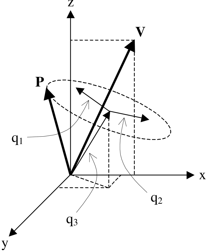
FIG. 8.: The variable $P_{y}(t)$ as a function of $\lambda(t)$, where $\lambda(t)$ varies linearly with time from $+\lambda$ to $-\lambda$, for adiabaticity parameters $\Upsilon=0.25$ (top left), $0.625$ (top right), $1.25$ (centre left), $3.125$ (centre right), $6.25$ (bottom left), and $18.75$ (bottom right). The parameters $D$ and $\beta$ are held constant at $D=0.02$ and $\beta=0.001$, and $P_{z}(t)\simeq 1$ throughout the evolution. The initial conditions are $P_{x}(0)\simeq P_{y}(0)\simeq 0$, and $P_{z}(0)\simeq 1$.

FIGURE 8

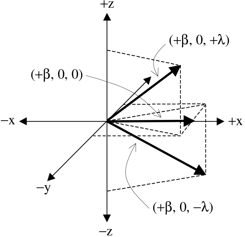
FIGURE 8

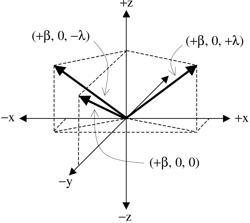
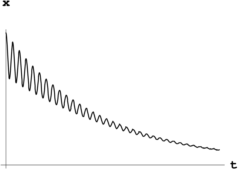
FIGURE 8

FIGURE 8

FIGURE 8

FIGURE 8

FIGURE 8

FIGURE 8

REFERENCES

- [1] B. H. J. McKellar and M. J. Thomson, Phys. Rev. D 49, 2710 (1994).
- [2] For foundational work see A. Dolgov, Sov. J. Nucl. Phys. 33, 700 (1981); R. A. Harris and L. Stodolsky, Phys. Lett. 116B, 464 (1982); L. Stodolsky, Phys. Rev. D 36, 2273 (1987); G. Raffelt, G. Sigl and L. Stodolsky, Phys. Rev. Lett 70, 2363 (1993); M. J. Thomson, Phys. Rev. A 45, 2243 (1992).
- [3] R. Foot and R. R. Volkas, Phys. Rev. D 55, 5147 (1997).
- [4] P. Di Bari and R. Foot, Phys. Rev. D 61, 105012 (2000).
- [5] R. Foot and R. R. Volkas, Phys. Rev. D 56, 6653 (1997); Erratum, ibid. D 59, 029901 (1999); R. Foot and R. R. Volkas, Astropart. Phys. 7, 283 (1997); N. F. Bell, R. Foot and R. R. Volkas, Phys. Rev. D 58, 105010 (1998); R. Foot, Astropart. Phys. 10, 253 (1999); P. Di Bari, P. Lipari and M. Lusignoli, Int. J. Mod. Phys. A 15, 2289 (2000); R. Foot and R. R. Volkas, Phys. Rev. D 61, 043507 (2000); P. Di Bari, Phys. Lett. B 482, 150 (2000).
- [6] R. Foot, M. J. Thomson and R. R. Volkas, Phys. Rev. D 53, 5349 (1996).
- [7] P. Langacker, University of Pennsylvania Preprint, UPR 0401T, September (1989); R. Barbieri and A. Dolgov, Phys. Lett. B 237, 440 (1990); Nucl. Phys. B349, 743 (1991); K. Enqvist, K. Kainulainen and J. Maalampi, Phys. Lett. B 244, 186 (1990); Nucl. Phys. B349, 754 (1991); K. Kainulainen, Phys. Lett. B 237, 440 (1990); K. Enqvist, K. Kainulainen and M. Thomson, Nucl. Phys. B373, 498 (1992); J. Cline, Phys. Rev. Lett. 68, 3137 (1992); X. Shi, D. N. Schramm and B. D. Fields, Phys. Rev. D 48, 2568 (1993); X. Shi, Phys. Rev. D 54, 2753 (1996); C. Y. Cardall and G. M. Fuller, Phys. Rev. D 54, 1260 (1996); D. P. Kirilova and M. V. Chizhov, Phys. Lett. B 393, 375 (1997); Nucl. Phys. B534, 447 (1998).
- [8] A. D. Dolgov, S. H. Hansen, S. Pastor and D. V. Semikoz, Astropart. Phys. 14, 79 (2000).
- [9] P. Di Bari, R. Foot, R. R. Volkas and Y. Y. Y. Wong, in preparation.
- [10] N. F. Bell, R. R. Volkas and Y. Y. Y. Wong, Phys. Rev. D 59, 113001 (1999).
- [11] L. Wolfenstein, Phys. Rev. D 17, 2369 (1978); ibid. 2634 (1979); S. P. Mikheyev and A. Yu. Smirnov, Nuovo Cimento C 9, 17 (1986).
- [12] See, for example, W. M. Itano, D. J. Heinzen, J. J. Bollinger and D. J. Wineland, Phys. Rev. A 41, 2295 (1990); E. Block and P. R. Berman, ibid. A 44, 1466 (1991); A. Beige and G. C. Hegerfeldt, ibid. A 53, 53 (1996).
- [13] D. Nötzold and G. Raffelt, Nucl. Phys. B307, 924 (1988).
- [14] C. P. Burgess and D. Michaud, Ann. Phys. 256, 1238 (1997).
- [15] K. S. M. Lee, R. R. Volkas and Y. Y. Y. Wong, companion paper, hep-ph/0007186.
- [16] K. S. M. Lee, University of Melbourne B. Sc. (Hons) thesis, (1999).
- [17] W. H. Press, S. A. Teukolsky, W. T. Vetterling and B. P. Flannery, Numerical Recipes: The Art of Scientific Computing, 2nd edition (Cambridge University Press, Cambridge, 1992).
- [18] X. Shi, Phys. Rev. D 54, 2753 (1996); K. Enqvist, K. Kainulainen and A. Sorri, Phys. Lett. B 464, 199 (1999); A. Sorri, Phys. Lett. B 477, 201 (2000).