AMES-HET-00-08

McGill-00/20

UdeM-GPP-TH-00-76

Supersymmetric Large Extra Dimensions
Are Small and/or Numerous
D. Atwood^a, C.P. Burgess^b, E. Filotas^b, F. Leblond^b,
D. London^c and I. Maksymyk^d
a Department of Physics and Astronomy, Iowa State University, Ames, Iowa 50011, USA.
^b Physics Department, McGill University,
3600 University St., Montréal, Québec, Canada, H3A 2T8.
^c Laboratoire René J.-A. Lévesque, Université de Montréal,
C.P. 6128, succ. centre-ville, Montréal, Québec, Canada, H3C 3J7.
^d Department of Physics, University of Maryland, College Park, Maryland 20742, USA.
Abstract

Recently, a scenario has been proposed in which the gravitational scale could be as low as the TeV scale, and extra dimensions could be large and detectable at the electroweak scale. Although supersymmetry is not a requirement of this scenario, it is nevertheless true that its best-motivated realizations arise in supersymmetric theories (like M theory). We argue here that supersymmetry can have robust, and in some instances fatal, implications for the expected experimental signature for TeV-scale gravity. The signature of the supersymmetric version of the scenario differs most dramatically from what has been considered in the literature because mass splittings within the gravity supermultiplet in these models are extremely small, implying in particular the existence of a very light spin-one superpartner for the graviton. We compute the implications of this graviphoton, and show that it can acquire dimension-four couplings to ordinary matter which can strongly conflict with supernova bounds.

1 Introduction

The recent transformation of the caterpillar of string theory into the butterfly of M-theory [1] has drawn considerable attention to the possibility that all known nongravitational particles might be trapped on a 4-dimensional surface, or brane, within a higher-dimensional ‘bulk’ spacetime [2, 3]. Most interestingly, the sizes of the extra dimensions could be quite large in this scenario, and the scale, $M_{s}$, describing gravitational interactions could be as low as several TeV. Because the fundamental scale might be so low, this is the first string ‘revolution’ to have reached experimental circles, stimulating considerable study of the potential experimental signatures of the extra-dimensional graviton [4, 5], which is present in all such models.

Our purpose here in this article is to explore the consequences of another particle — a bosonic superpartner of the graviton — whose existence in this scenario is almost as robust as that of the graviton itself. All that is required is the presence of supersymmetry. Furthermore, this particle is extremely light (potentially as low as $m\mathrel{\raise 1.29167pt\hbox{$<$\kern-7.5pt\lower 4.30554pt\hbox{$\sim$}}}1$ eV) even if all supersymmetries are spontaneously broken. Although, strictly speaking, supersymmetry is not a necessary requirement for brane models, it is a feature of M-Theory, as well as being present in an overwhelming majority of the explicit field-theory realizations of the brane-world scenario which have been proposed.

Supersymmetry enters the phenomenology of brane models in an unusual way. This is because such models deal with the heirarchy problem differently than had been done previously. In particular, there is no requirement that the mass splitting between particles and their superpartners be much smaller than the gravitational scale. Furthermore, branes themselves tend to break supersymmetries, and so could naturally produce a nonsupersymmetric low-energy spectrum at scales below a TeV. It is tempting to conclude from these considerations that supersymmetry should therefore be irrelevant to — or have very model-dependent implications for — experiments.

The robust signal which we explore here is based on the observation that even if the supersymmetry breaks strongly on the brane, at scale $M_{s}$, the mass splittings which this implies within the graviton supermultiplet are much smaller, of order $M^{2}_{s}/M_{p}$, where $M_{p}\sim 10^{19}$ GeV is the usual four-dimensional Planck mass. Since the graviton is massless, this sets an upper bound to the masses of its superpartners. This upper bound can be extremely low, being $\mathrel{\raise 1.29167pt\hbox{$<$\kern-7.5pt\lower 4.30554pt\hbox{$\sim$}}}1$ eV if $M_{s}\sim 1$ TeV.

Furthermore, because the graviton lives in the bulk space, its supermultiplet is a supermultiplet for a higher-dimensional supersymmetry. From the four-dimensional perspective, this means that the graviton supermultiplet is necessarily a representation of extended supersymmetry, having at least two supersymmetry generators. The smallest such multiplet involves two spin-3/2 gravitini, $\psi^{a}_{\mu}$, and one spin-1 boson, $V_{\mu}$, in addition to the graviton. We are therefore led on quite general grounds to the existence of a very light bulk-space spin-one boson — which we call the graviphoton, following the early extended-supersymmetry literature — in addition to the graviton and the (two or more) gravitini. Better yet, the couplings of this spin-1 particle can be universal and of gravitational strength, since they are related to those of the graviton by supersymmetry.

In this paper we focus on the properties of the graviphoton, and explore its experimental implications. We identify its dominant low-energy couplings and show how these change the predictions of graviton exchange. Depending on the values taken by these couplings, graviphoton exchange can alter the expected signal of large extra dimensions quite dramatically. In particular, low-energy Standard-Model gauge symmetries permit the graviphoton to have dimension-four interactions with Standard-Model particles once supersymmetry breaks, and so these couplings can dominate those of the graviton at low energies. If such couplings are present, we find that the rate they predict for graviphoton emission can have catastrophic effects for supernovae, implying bounds for the underlying gravity scale, $M_{s}$, which can be as large as $10^{10}$ GeV for $n=2$ extra dimensions. TeV-scale strings can be ruled out in this case for $n<5$.

We present our results as follows. First, in Sec. 2, we outline the properties of the graviton supermultiplet and its couplings to ordinary particles. We pay particular attention to the lowest-dimension couplings it may have, and how large these might be expected to be from the microscopic point of view. We identify two kinds of couplings to fermions, which differ by whether or not the corresponding interactions are derivatively coupled. The nonderivative couplings are the ones which are potentially dangerous for supernovae, and we estimate their size in this section. Next, in Sec. 3, we compute the graviphoton production rate in fermion-antifermion collisions. If the lowest-dimension couplings are suppressed by derivatives, then we find production rates which are of order $\sigma\sim E^{n}/M_{s}^{n+2}$, comparable to those computed elsewhere for gravitons [4]. If they are not so suppressed, then the production rates are instead $\sigma\sim E^{n-2}/M_{s}^{n}$, and so can be much higher at low energies. Sec. 4 then calculates the implications of these production cross sections for supernova bounds, with the result that non-derivative couplings are very strongly constrained. Sec. 5 describes the effects of virtual graviphoton exchange on fermion scattering, and examines potential signals in accelerator experiments. Although the graviphoton is easily distinguished from the graviton [5] in these processes, both cannot be disentangled from other states having mass $M_{s}$ (such as string oscillator modes [6]), complicating the statement of what experiments should see. Finally, our conclusions are summarized in Sec. 6.

2 Graviphoton Properties

We first describe the mass and couplings of the graviphoton, $V_{\mu}$, focussing on those features which are model independent. We do so first from a low-energy four-dimensional perspective, and then repeat the discussion from a higher-dimensional point of view. As we will see, although one can make fairly general statements about the size of the graviphoton couplings to ordinary matter, specific details are necessarily model dependent. (This is in contrast to graviton couplings to matter, which are determined by the general covariance of the theory.) Furthermore there are, unfortunately, no realistic brane models, so one cannot even present a sample calculation of the graviphoton couplings. Thus, at present, the discussion of these couplings remains essentially at the level of dimensional analysis.

2.1 Graviphoton Mass

The most robust prediction possible is for the size of the graviphoton mass, since this follows purely on the grounds of symmetry. (The mass of interest in the present instance is the extra-dimensional mass, $m_{\scriptscriptstyle V}$, which is common to all Kaluza-Klein modes.) The extended supersymmetry of the bulk space (or gravitational sector) implies two key properties for the graviphoton. First, since it is related to the massless graviton by supersymmetry, this graviphoton mode remains massless so long as the four-dimensional extended supersymmetry remains unbroken. Second, its coupling to any supersymmetry-breaking sector is of gravitational strength. It follows that if supersymmetry is broken by an expectation value of order $M_{s}^{2}$, then $m_{\scriptscriptstyle V}\mathrel{\raise 1.29167pt\hbox{$<$\kern-7.5pt\lower 4.30554pt\hbox{$\sim$}}}M_{s}^{2}/M_{p}$. For $M_{s}\sim 1$ TeV we have $m_{\scriptscriptstyle V}\mathrel{\raise 1.29167pt\hbox{$<$\kern-7.5pt\lower 4.30554pt\hbox{$\sim$}}}10^{-3}$ eV.

Because the graviphoton lives in the bulk, from the four-dimensional viewpoint it breaks up into a tower of Kaluza-Klein (KK) states. Each of these states has a mass of order

$$M_{l}^{2}=m_{\scriptscriptstyle V}^{2}+{k_{l}\over r^{2}},$$ (2.1)

where $r$ is a measure of the linear size of the extra dimensions and $k_{l}$ is a constant depending on the extra-dimensional geometry and on the quantum numbers, $l$, of the mode in question. Since $r$ is related to the brane scale, $M_{s}$, and the Planck mass, $M_{p}$, by

$$M_{p}\sim(M_{s}\,r)^{n/2}\;M_{s},$$ (2.2)

for $n$ extra dimensions, we typically have the heirarchy $m_{\scriptscriptstyle V}\ll 1/r\ll M_{s}$.

2.2 Effective Trilinear Couplings

At a microscopic level, given an explicit brane model, the graviphoton couplings to particles may be read directly off from the model’s action. These couplings may then be evolved down to the effective four-dimensional effective theory describing the particles we know by integrating out all of the model’s heavy or invisible degrees of freedom. Given that the brane scale, $M_{s}$, is a TeV or more, it is only the effective couplings of this low-energy theory which are probed in experiments.

When discussing graviphoton couplings to ordinary matter it is therefore useful to separate the discussion into two parts. First, we may identify those effective interactions which have lowest dimension and which are consistent with all of the known low-energy symmetries. These will govern the phenomenological properties of the graviphoton. We identify these couplings in the present section. Next, we may ask how big these couplings are predicted to be in realistic brane models. This is the topic of the next subsections. The absence of detailed realistic constructions [7] makes the second step more difficult to perform, and we therefore limit ourselves in these sections to what may be said on fairly general grounds.

In the effective four-dimensional theory the graviphoton may be regarded as a tower of $U(1)$ gauge bosons, $V_{l}^{\mu}$ (with $l=1,2,\dots$ labelling the various KK modes), whose gauge symmetries commute with the electroweak gauge group. At scales below the electroweak symmetry-breaking scale, the effective theory need not linearly realize $SU_{\scriptscriptstyle L}(2)\times U_{\scriptscriptstyle Y}(1)$, and so the lowest-dimension couplings arise at dimension 4:

$${\cal L}_{\rm dim\,4}=i\overline{\psi}\gamma_{\mu}(\hat{g}^{l}+\hat{g}^{l}_{5}\gamma_{5})\psi^{\prime}\;V_{l}^{\mu}-{\hat{\epsilon}_{la}\over 2}\;F^{a}_{\mu\nu}\,V_{l}^{\mu\nu}-\hat{\lambda}_{l}\;W_{\mu}^{*}\,W_{\nu}\;\partial^{\mu}V_{l}^{\nu},$$ (2.3)

where $\psi,\psi^{\prime}$ denote the various fermions of the effective theory, and $F^{a}_{\mu\nu}$ is the field strength for any of the low-energy spin-one particles, which are labelled by the index ‘$a$’ (e.g.: $a$ could represent the photon and the $Z$, if these are all in the effective theory). Here and in what follows a caret over a coupling constant is meant to emphasize that it is the four-dimensional coupling to a particular KK mode, as opposed to the higher-dimensional coupling between the respective fields.

Note that the coupling of two graviphotons to an ordinary gauge boson is suppressed on general grounds by Yang’s theorem, which precludes low-energy interactions of the form $XVV$, where $X=Z,W$ or $\gamma$. The lowest-dimension trilinear coupling which is possible is that shown in Eq. (2.3), where $\hat{\lambda}_{l}\mathrel{\raise 1.29167pt\hbox{$<$\kern-7.5pt\lower 4.30554pt\hbox{$\sim$}}}e^{2}v^{2}/(M_{s}M_{p})$ is an upper limit for the order of magnitude expected for the relevant effective coupling of any one KK mode. Here $v=246$ GeV is the order parameter for electroweak gauge-symmetry breaking, and appears because of the necessity to break this symmetry in order to generate the interaction in Eq. (2.3).

The quantities $\hat{g}^{l}$ and $\hat{g}^{l}_{5}$ describe the quantum numbers of the low-energy fermions under the $U(1)$ groups gauged by the graviphotons, $V_{l}^{\mu}$, and would all vanish if all such fermions were neutral under these $U(1)$’s. Even if this were so, they would be regenerated if the couplings $\hat{\epsilon}_{la}$ were nonzero, since these induce a mixing amongst the spin-one particles which can induce a coupling of the $V_{l}^{\mu}$’s to ordinary fermions. For instance, for energies for which we can neglect the masses of the graviphoton modes, diagonalization of graviphoton-photon mixing produces a coupling of the form

$${\cal L}_{\rm ind}=-\;{\hat{\epsilon}_{l\gamma}\over 2}\;V_{l}^{\mu}J_{\mu}^{\rm em},$$ (2.4)

where $J^{\rm em}_{\mu}$ denotes the usual electromagnetic current, resulting in contributions to the $V$-fermion couplings of order $\delta\hat{g}^{l}_{5}=0$, $\delta\hat{g}^{l}=-\frac{e}{2}\,\hat{\epsilon}_{l\gamma}\,Q$, with $Q$ denoting the fermion electric charge (normalized such that $Q=1$ for the proton).

Since dimension-four couplings are dimensionless in four spacetime dimensions, it is tempting to hope that the couplings $\hat{g},\hat{g}_{5}$ and $\hat{\epsilon}$ might be unsuppressed by powers of $1/M_{p}$. Although logically possible, this hope is unlikely to be fulfilled in real brane models, as we shall see once the microscopic origin of these couplings is traced to its higher-dimensional roots. In subsequent sections we instead find these couplings naturally have the size $(M_{s}\,r)^{-n/2}\sim M_{s}/M_{p}$. Although these are extremely small couplings they convert, as usual, to powers of $M_{s}$ once summed over the contributions of all KK modes.

For energies above the electroweak symmetry-breaking scale, but below the threshold for other particles — such as for superpartners if there is a low-energy four-dimensional supersymmetry — interactions like those of Eq. (2.3) are also possible provided that they also linearly realize the electroweak gauge group. The possible dimension-four interactions then become:

$${\cal L}_{\rm dim\,4}=i\overline{\psi}\gamma_{\mu}(\hat{\tilde{g}}^{l}+\hat{\tilde{g}}^{l}_{5}\gamma_{5})\psi^{\prime}\;V_{l}^{\mu}-{\hat{\tilde{\epsilon}}_{l}\over 2}\;B_{\mu\nu}\,V_{l}^{\mu\nu},$$ (2.5)

where all fermions in the same electroweak representation must carry the same graviphoton charge, and $B_{\mu\nu}$ is the field strength for the $U_{\scriptscriptstyle Y}(1)$ factor of the electroweak gauge group. Eq. (2.5) implies Eq. (2.3) with relations amongst the effective couplings, such as $\hat{\epsilon}_{l\gamma}=\hat{\tilde{\epsilon}}_{l}\,c_{w}$ and $\hat{\epsilon}_{l{\scriptscriptstyle Z}}=-\hat{\tilde{\epsilon}}_{l}\,s_{w}$, where $s_{w}=\sin\theta_{\scriptscriptstyle W}$ (or $c_{w}=\cos\theta_{\scriptscriptstyle W}$) is the sine (or cosine) of the usual weak mixing angle.

The graviphoton coupling to gauge bosons, $\hat{\lambda}_{l}$, does not arise at all at dimension four, but does appear once dimension-six electroweak-invariant effective operators are considered. This leads to the previously-quoted estimate of the coefficient $\hat{\lambda}_{l}\sim e^{2}v^{2}/(M_{s}M_{p})$, where $v=246$ GeV is the usual Higgs expectation value.

More interactions are possible at dimension five, of which we consider here only the fermion-graviphoton couplings as being of most practical interest. These can have the electric/magnetic moment form:

$${\cal L}_{\rm dim\,5}=i\overline{\psi}\gamma_{\mu\nu}(\hat{a}_{l}+i\hat{b}_{l}\gamma_{5})\psi^{\prime}\;\partial^{\mu}V_{l}^{\nu}+\hbox{other terms}.$$ (2.6)

Unless this interaction is forbidden by a low-energy symmetry, it can be expected to be present with at most gravitational strength, $\hat{a}_{l},\hat{b}_{l}\mathrel{\raise 1.29167pt\hbox{$<$\kern-7.5pt\lower 4.30554pt\hbox{$\sim$}}}1/M_{p}$, although it is typically smaller than this upper limit. There are at least two low-energy symmetries which can act to dramatically reduce the size of these couplings. First, to the extent that graviphoton interactions preserve CP (as might be expected if they are related to graviton couplings by supersymmetry), the effective couplings $\hat{b}_{l}$ must vanish.

Second, since the Standard-Model fermion quantum numbers forbid writing a similar dimension-five term which linearly realizes the electroweak gauge symmetry, an electroweak-invariant version of Eq. (2.6) first arises at dimension six. If only Standard Model fermions (or others for which Eq. (2.6) is also forbidden) are present in the low-energy theory, then the effective couplings $a_{l}$ and $b_{l}$ should be at most $a_{l},b_{l}\mathrel{\raise 1.29167pt\hbox{$<$\kern-7.5pt\lower 4.30554pt\hbox{$\sim$}}}v/(M_{s}M_{p})$. Of course further suppressions, such as by small mixing angles or loop factors, are also not ruled out.

As we shall see, there are microscopic theories for which some fermions can acquire couplings $\hat{a}_{l}\sim O(1/M_{p})$. This can happen if the low-energy theory may contain nonstandard fermions — such as gauginos or mirror fermions, for instance — whose quantum numbers permit forming the interaction of Eq. (2.6) without violating electroweak invariance. Since the effective couplings which these imply for ordinary fermions are typically suppressed by powers of small mixing angles or loop factors, we regard the estimate $\hat{a}_{l},\hat{b}_{l}\mathrel{\raise 1.29167pt\hbox{$<$\kern-7.5pt\lower 4.30554pt\hbox{$\sim$}}}v/(M_{s}M_{p})$ as a fairly optimistic upper limit.

2.3 Microscopic Couplings

We now consider how the above effective couplings might arise from more microscopic, higher-dimensional physics. In the absence of detailed realistic brane models [7] our discussion is necessarily tentative, and we focus only on drawing conclusions which follow from reasonably general arguments. For simplicity we also restrict ourselves here to the more traditional scenario, with TeV-scale gravity associated with very large extra dimensions [2], as opposed to the alternative scenario [3] in which TeV-scale gravity arises with gravity localized near our brane.

The size expected for the low-energy effective couplings described above largely depends on how the model in question answers the following two questions:

1. Which of the observed low-energy particles are confined to the brane? The possibility of lowering the gravity scale below $M_{p}$ ultimately arises because spin-one particles are trapped on our brane while gravitational forces are not. This allows long-range gauge forces, like electromagnetism, to ‘see’ fewer large dimensions than does gravity, and so changes the connection between Newton’s constant (or $M_{p}$) and the fine-structure constant, $\alpha$, on one hand, and the underlying coupling constants and gravity scale, $M_{s}$, on the other. We therefore require all light spin-one particles to be confined to our brane.

   It is then natural, and is usually taken to be true in the literature, to assume that all light fermions should also be confined to the brane (see, however, Ref. [8]). Although this is the simplest possibility, it is not logically required, and so in what follows we contrast the usual assumption with what would heppen if some light fermions were to live in the bulk.

2. How many supersymmetries survive below $M_{s}$ on our brane? Since our starting point in this paper assumes the underlying theory is supersymmetric we must ask how many supersymmetries survive amongst observable particles in the low-energy theory. Although the splitting of the gravity multiplet in the bulk space is necessarily suppressed by gravitational strength interactions, there are two main alternatives for the splitting of supermultiplets on the brane:

   1. Supersymmetry is completely broken on our brane at scale $M_{s}$, and so observable brane states do not have superpartners in the low-energy theory. In this instance the low-energy brane spectrum could be just the observed Standard Model fields and no more, although other exotic light states are logically possible.

   2. At least one supersymmetry survives on the brane below the scale $M_{s}$, and so the low-energy effective theory contains superpartners for all of the observed particles. In this case the low-energy brane world might be expected to resemble the supersymmetric Standard Model, although probably with a specific form for the soft supersymmetry breaking interactions. Again the existence of exotic low-energy supermultiplets is not ruled out in this scenario.

2.3.1 Couplings to Brane Particles

First imagine that all of the relevant low-energy particles are confined to our brane (except, of course, for the graviton supermultiplet). To be concrete, suppose that we denote the spacetime coordinates by $\{x^{\mu},y^{m}\}$, where the $x^{\mu}$ label the dimensions parallel to our brane, and $y^{m}$ label the transverse dimensions. We further choose the position of our own brane to be given by the condition $y^{m}=0$. In this case then we must restrict all graviphoton couplings to have the form:

$${\cal L}_{4+n}=-\frac{1}{4}\;V_{\mu\nu}\,V^{\mu\nu}+{\cal L}_{4}[\psi(x),V(x,y);M_{s}]\;\delta^{n}(y),$$ (2.7)

where $\psi(x)$ collectively denotes all brane fields, while $V^{\mu}(x,y)=\sum_{l}V^{\mu}_{l}(x)\,u_{l}(y)$ denotes the extra-dimensional graviphoton field, having field strength $V_{\mu\nu}=\partial_{\mu}V_{\nu}-\partial_{\nu}V_{\mu}$. The functions $u_{l}(y)$ here denote an appropriate complete set of Kaluza-Klein mode functions for the extra dimensions, most of whose details play no role in what follows [9]. They are assumed to be normalized to preserve the canonical normalization of the KK modes, $V_{l}^{\mu}$, i.e.:

$$\int d^{n}y\;u_{k}(y)\,u_{l}(y)=\delta_{kl},$$ (2.8)

where $d^{n}y$ denotes the appropriate covariant measure. For the present purposes it suffices to notice that this normalization implies the mode functions, $u_{l}(y)$, scale like $r^{-n/2}$ if $r$ denotes the linear size of the extra dimensions.

The properties assumed for ${\cal L}_{4}$ are these: ($i$) it is assumed to contain only $M_{s}$ as its basic dimensional scale; ($ii$) it is assumed to linearly realize the electroweak gauge group, $SU_{\scriptscriptstyle L}(2)\times U_{\scriptscriptstyle Y}(1)$; ($iii$) if the low-energy brane theory should also contain superpartners for the Standard Model fields, then ${\cal L}_{4}$ is assumed to be supersymmetric. With these assumptions the expected sizes for the low-energy effective couplings can be made explicit.

Suppose first that only Standard Model fields are included. In this case no symmetries forbid the appearance of the dimension-four couplings of Eq. (2.5). Whether they appear or not at tree level therefore depends explicitly on whether or not Standard Model particles carry nonzero charges for the graviphoton’s $U(1)$ gauge symmetry. If these are nonzero, then dimensional analysis determines the size of the effective four-dimensional couplings as follows. Since these couplings are linear in $V^{\mu}$ they must be proportional to one factor of the mode functions $u_{k}(y)$, which must be evaluated at $y=0$ because of the delta function in Eq. (2.7). It follows that the couplings scale with the radius of the extra dimensions in the same way as do the $u_{k}$’s: $\hat{g}_{l}\sim g\,r^{-n/2}$, where $g$ denotes the graviphoton coupling constant in the higher-dimensional theory. Since $M_{s}$ supplies all of the missing dimensions by assumption, dimensional analysis implies $g\propto M_{s}^{-n/2}$ and so we see that $\hat{g}_{l},\hat{g}_{5l}$ (and $\hat{\epsilon}$) are all of order $(M_{s}r)^{-n/2}\sim M_{s}/M_{p}$, as advertised earlier. If the extra dimensions are torii then $u_{k}(y=0)$ is also independent of the mode index, $k$, implying trilinear couplings of equal strength to all of the KK modes.

It should be remarked that even if the graviphoton charges for the observed fermions should vanish for Standard Model fermions in the underlying higher-dimensional theory, they will be generated through loops unless this is precluded by another symmetry of the brane model of interest. A concrete way in which loop-generated charges could arise concretely, for instance, is through the generation of the off-diagonal vacuum polarization $B_{\mu\nu}\;V^{\mu\nu}$ by loops of any brane states which do carry nonzero charges for both graviphotons and ordinary $U_{\scriptscriptstyle Y}(1)$ hypercharge. Notice that the particles circulating in this loop can have large masses, of order $M_{s}$ or larger, because their contributions to the kinetic terms need not decouple since these have dimension four in the four-dimensional theory. In this case one might expect $\hat{e}g\sim\hat{\epsilon}$ to be suppressed by loop factors, although not by powers of the mass of the particle in the loop.

Similar considerations apply to the higher-dimensional interactions. In this case direct magnetic/electric moment graviphoton couplings to fermions of the form of Eq. (2.6) are precluded until dimension six, since a power of the Higgs field is required by electroweak gauge invariance. One therefore expects couplings of order $(v/M_{s}^{2})\;(M_{s}r)^{-n/2}\sim v/(M_{s}M_{p})$, as advertised earlier. Additional suppressions by mixing angles or loops may also be present, depending on how the couplings to Standard-Model fermions arise.

The suppression of the magnetic-moment type interactions by powers of $v$ need not arise if nonstandard fermions are also present in the spectrum on the brane. For instance if the weak-scale theory contains mirror fermions in addition to those of the Standard Model, then these fermions and their mirror pairs can form magnetic moment graviphoton couplings without gauge invariance requiring the presence of a Higgs v.e.v., $v$. The same is true for sfermions, such as gauginos, which lie in real representations of the electroweak gauge group. Fermions such as these are allowed interactions as in Eq. (2.6) with couplings of order $(M_{s}r)^{-n/2}\sim M_{s}/M_{p}$, without the additional factor of $v/M_{s}$. Other ordinary fermions can then acquire both dimension five and dimension four graviphoton couplings through mixings or loops involving these particles.

2.3.2 Couplings to Bulk Particles

It is not ruled out that some of the more weakly-interacting low-energy particles — such as right-handed neutrinos, for instance [8] — might arise microscopically as particles which can propagate off the brane into the bulk. In this section we estimate the sizes to be expected for the effective couplings if some fermions are bulk-space fields.

For bulk space fields the $r$-dependence of the effective couplings differs from that predicted by Eq. (2.7) in two ways. First, these interactions involve an integration over the extra dimensions due to the absence of the delta function $\delta^{n}(y)$. Second, the bulk-space fields are themselves KK towers of modes, $\psi(x,y)=\sum_{l}\psi_{l}(x)\eta_{l}(y)$, with canonical normalization requiring $\eta_{l}\propto r^{-n/2}$, just as for the graviphoton. (It is the presence of these KK modes, split only by masses of order $1/r$, which permits this possibility only for sufficiently weakly-coupled fermions.)

The couplings of such modes are also more restricted since they are constrained by all of the spacetime symmetries and supersymmetries of the bulk space itself. Since the bulk space enjoys extended supersymmetries from the four-dimensional point of view, the effective couplings of such states to the graviphoton are easily identified using the known properties of extended supersymmetric models in four dimensions.

In this case the tree-level effective couplings may be obtained from inspection of the $N=2$ supergravity couplings in four spacetime dimensions [10]. We find in this way vanishing dimension-four couplings, $g=g_{5}=\epsilon=0$, and universal magnetic moment couplings:

$${\cal L}_{v}=i\kappa_{v}\overline{\psi}\gamma^{\mu\nu}\psi^{\prime}\;\partial_{\mu}V_{\nu},$$ (2.9)

with $\kappa_{v}=c/M_{s}^{1+n/2}$, which are related by supersymmetry transformations of the universal gravitational couplings:

$${\cal L}_{h}=2i\kappa\;h^{\mu\nu}\overline{\psi}\gamma_{\mu}{\leftrightarrow\atop{}}{\kern-8.00003pt\partial_{\nu}}\,\psi,$$ (2.10)

where (for our purposes) $\kappa=1/M_{s}^{1+n/2}$ can be taken to define the scale $M_{s}$.

We see that the additional symmetry implies lowest-dimensional trilinear four-dimensional graviphoton couplings which are universal and which preserve C, P and CP. Electroweak invariance is satisfied in this case because four-dimensional $N=2$ supermultiplets necessarily contain only real representations of the gauge group, implying the presence of whatever mirror particles are required to permit the coupling of Eq. (2.9).

Notice that the couplings of Eq. (2.9) must exist at tree level for any bulk-space spin-half particles, so if any such particles carry electroweak quantum numbers the effective dimension-four $B_{\mu\nu}-V_{\mu\nu}$ mixing is inevitably generated through loops.

3 Production Rates

We now turn to a discussion of the phenomenological consequences of the effective couplings of Eqs. (2.3) and (2.6). Direct graviphoton production is the topic of this section, while the influence of graviphoton exchange is pursued in the Sec. 5.

Graviphoton production is very similar to graviton production, which has been discussed extensively in the literature within the framework of large extra dimensions [4]. The observable in both cases is missing energy produced in association with other observed particles, such as photons. The main conclusion we draw in this section is that graviphoton production can change the graviton signal in an important way, for two reasons. First, the graviphoton can couple with a strength which is less suppressed by powers of $E/M_{s}$ than can the graviton, and so production of graviphotons can easily dominate the graviton signal. It is this property which plays the central role in the next section’s discussion of supernova bounds. Second, since the graviphoton has unit spin, it contributes differently to observables which depend on the spin of the unobserved particle, and so the production of these two types of particles can be distinguished from one another, in principle, should it occur at an observable level.

Figure 1: The Feynman graphs contributing to photon-graviphoton production. The graviphoton-fermion interaction here is a sum of the dimension-four helicity-preserving interaction of Eq. (2.3) and the dimension-five helicity-flipping interaction of Eq. (2.6).

3.1 Cross Section Formulae

Graviphoton emission in fermion-antifermion collisions is mediated by the Feynman graphs of Fig. (1), for which the graviphoton-fermion couplings can be either the helicity-preserving dimension-four couplings of Eq. (2.3) or the helicity-flipping dimension-five couplings of Eq. (2.6). Because of their different helicity properties these two kinds of couplings do not interfere with one another in the production cross section (in the limit where fermion masses are neglected), so $d\sigma=d\sigma_{\rm dim\,4}+d\sigma_{\rm dim\,5}$.

So long as the centre-of-mass energy, $E$, of the production process is much higher than the inverse radius of the extra dimensions, i.e. $Er\gg 1$, the production cross section can be computed in either of two equivalent ways. It may be computed in four dimensions (by summing over the contributions of each of the many KK states) or the calculation may be done directly in higher dimensions, with the graviphoton represented by a single higher-dimensional field. In either case explicit evaluation of the graphs in Figure (1) gives the following expressions for the (unpolarized) reaction $f\overline{f}\to\gamma V$:

$${d\sigma_{\rm dim\,4}\over du\,dt\,dM^{2}} = -\,{\alpha\,Q^{2}_{f}\,(g^{2}_{f}+g^{2}_{5f})\over 2\,N_{f}\,s^{2}}\;\left({u\over t}+{t\over u}+{2\,M^{2}s\over u\,t}\right)\,P_{n}\,\delta(s+t+u-M^{2}),$$ (3.1)

$${d\sigma_{\rm dim\,5}\over du\,dt\,dM^{2}} = -\,{\alpha\,Q_{f}^{2}\,(a_{f}^{2}+b_{f}^{2})\over 4\,N_{f}\,s^{2}}\;\left[{(s^{2}+M^{4})\,M^{2}-4ut(u+t)\over ut}\right]\,P_{n}\,\delta(s+t+u-M^{2}).$$

Here $g_{f},g_{5f}\sim M_{s}^{-n/2}$ and $a_{f},b_{f}\sim M_{s}^{-1-n/2}$ are the higher-dimensional coupling constants while $P_{n}$ denotes the $n$-dimensional phase-space factors, $P_{n}=\Omega_{n}\,M^{n-2}/[2(2\pi)^{n}]$, with $\Omega_{n}=2\pi^{n/2}/\Gamma(n/2)$ representing the volume of the $(n-1)$-sphere. $M$ represents the invariant (four-dimensional) mass against which the photon recoils. $N_{f}$ is the number of colours carried by the initial fermion, and $s,t$ and $u$ are the usual four-dimensional Mandelstam variables, related to the four-momenta of the particles involved by $s=-(p_{f}+p_{\overline{f}})^{2}$, $t=-(p_{f}-p_{\gamma})^{2}$ and $u=-(p_{f}-p_{\scriptscriptstyle V})^{2}$. This cross section was derived assuming the extra dimensions to be an $n$-dimensional torus, although the dependence on this assumption is weak for most values of the parameters [9].

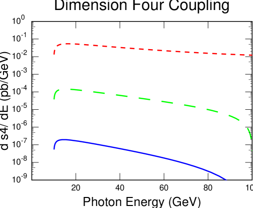
Figure 2: The differential cross section for $e^{+}e^{-}\to\gamma+GP$, against photon energy, due to the dimension-four couplings of Eq. (2.3). The plot assumes an initial electron energy $E_{e}=100$ GeV, a minimum photon transverse energy $\omega_{\scriptscriptstyle T}\geq 10$ GeV, and $M_{s}=1000$ GeV. The solid line uses $n=6$, the long-dashed line $n=4$ and the short-dashed line $n=2$.

In terms of the photon energy, $\omega$, and scattering angle, $\theta$, relative to the incoming fermion direction (in the CM frame) these expressions become:

$${d\sigma_{\rm dim\,4}\over dx\,dc} = {\alpha\,Q^{2}_{f}\,(g^{2}_{f}+g^{2}_{5f})\;E^{n-2}\over 8\pi^{n/2}\,\Gamma(\frac{n}{2})N_{f}}\;\;\Bigl{(}1-x\Bigr{)}^{n/2-1}\;\left({x^{2}(1+c^{2})+4(1-x)\over x(1-c^{2})}\right),$$

$${d\sigma_{\rm dim\,5}\over dx\,dc} = {\alpha\,Q_{f}^{2}\,(a_{f}^{2}+b_{f}^{2})E^{n}\over 2\pi^{n/2}\,\Gamma(\frac{n}{2})\,N_{f}}\;(1-x)^{n/2-1}\left[{(1-x)(2-2x+x^{2})+x^{3}(1-c^{2})\over x(1-c^{2})}\right],$$ (3.3)

where $x=\omega/E_{e}$, $E_{e}$ is the incoming electron energy and $c\equiv\cos\theta$.

When comparing with experiments, these expressions must be added to those for the cross section for photon-graviton production, $f\overline{f}\to\gamma g$, which has been calculated in Refs. [4], whose results we reproduce here (using our conventions) for convenience of reference:

$${d\sigma_{\rm g}\over dx\,dc}={\alpha\,Q_{f}^{2}\,\kappa^{2}\,E^{n}\over 16\pi^{n/2}\,\Gamma(\frac{n}{2})\,N_{f}}\;(1-x)^{n/2-1}\left[{(2-x)^{2}(1-x+x^{2})-3x^{2}\,c^{2}(1-x)-x^{4}c^{4}\over x(1-c^{2})}\right],$$ (3.4)

where $\kappa=1/M_{s}^{1+n/2}$.

Figures (2) through (5) plot the singly-differential cross sections, which are obtained by integrating Eqs. (3.1). The collinear mass singularities associated with the neglect of the electron mass in these expressions is excluded by the physical requirement that the photon have a minimum transverse energy, $\omega_{\scriptscriptstyle T}\geq 10$ GeV.

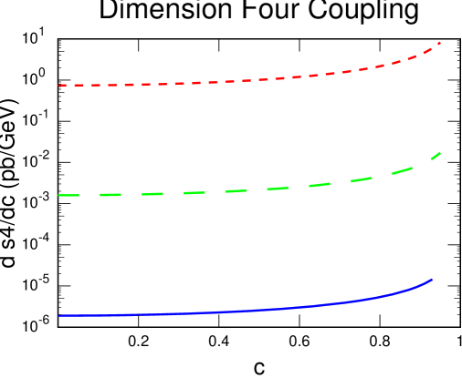
Figure 3: The differential cross section for $e^{+}e^{-}\to\gamma+GP$, against photon scattering angle in the CM frame, arising due to the dimension-four couplings of Eq. (2.3). The plot assumes an initial electron energy $E_{e}=100$ GeV, a minimum photon transverse energy $\omega_{\scriptscriptstyle T}\geq 10$ GeV, and $M_{s}=1000$ GeV. The solid line uses $n=6$, the long-dashed line $n=4$ and the short-dashed line $n=2$.

The total production cross section due to the dimension-four interactions becomes:

$$\sigma_{\rm dim4}=k_{n}\;\left({E\over 100\,\hbox{GeV}}\right)^{n-2}\;\left({g_{f}^{2}+g_{5f}^{2}\over(1\,\hbox{TeV})^{-n}}\right),$$ (3.5)

with

$$k_{n}=\cases{3.5~{}{\rm pb}~{},&$n=2$ ~{},\cr 0.18~{}{\rm pb}~{},&$n=3$ ~{},\cr 7.5\times 10^{-3}~{}{\rm pb}~{},&$n=4$ ~{},\cr 2.7\times 10^{-4}~{}{\rm pb}~{},&$n=5$ ~{},\cr 8.8\times 10^{-6}~{}{\rm pb}~{},&$n=6$ ~{},\cr}$$ (3.6)

while the corresponding result using the dimension-five interactions is:

$$\sigma_{\rm dim5}=\tilde{k}_{n}\;\left({E\over 100\,\hbox{GeV}}\right)^{n}\;\left({a_{f}^{2}+b_{f}^{2}\over(1\,\hbox{TeV})^{-n+2}}\right),$$ (3.7)

with

$$\tilde{k}_{n}=\cases{0.051~{}{\rm pb}~{},&$n=2$ ~{},\cr 2.7\times 10^{-3}~{}{\rm pb}~{},&$n=3$ ~{},\cr 1.1\times 10^{-4}~{}{\rm pb}~{},&$n=4$ ~{},\cr 4.2\times 10^{-6}~{}{\rm pb}~{},&$n=5$ ~{},\cr 1.4\times 10^{-7}~{}{\rm pb}~{},&$n=6$ ~{}.\cr}$$ (3.8)

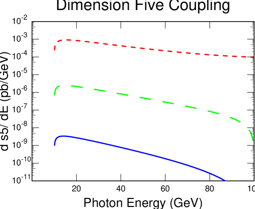
Figure 4: The differential cross section for $e^{+}e^{-}\to\gamma+GP$, against photon energy, due to the dimension-five couplings of Eq. (2.6). The plot assumes an initial electron energy $E_{e}=100$ GeV, a minimum photon transverse energy $\omega_{\scriptscriptstyle T}\geq 10$ GeV, and $M_{s}=1000$ GeV. The solid line uses $n=6$, the long-dashed line $n=4$ and the short-dashed line $n=2$.

These results are to be compared with Standard Model background processes, which are principally due to $\gamma-Z$ emission, with the $Z$ subsequently decaying invisibly into neutrinos, as has been discussed in detail for graviton production in Refs. [4].

3.2 Discussion

The property of the production cross sections which is central to the remaining discussions is its dependence on the centre-of-mass energy. This dependence is a simple power law – being proportional to $E^{n}/M_{s}^{n+2}$ for both the graviton and the magnetic-moment graviphoton interactions. The simple power-law behaviour is typical of low-energy effective interactions, and arises in the present case due to the derivative nature of both of these couplings. By contrast, the energy dependence of the dimension-four graviphoton production cross section is $E^{n-2}/M_{s}^{n}$. This means that this coupling is suppressed by two fewer powers of $E/M_{s}$ than are the others. This observation has several consequences.

1. All other things being equal, at low energies the dimension-four graviphoton couplings must dominate, and their domination is stronger the lower the energy of interest. This makes them particularly important for supernovae bounds, for which the relevant processes involve energies of order 10 MeV.

2. For the same reason production rates for graviphotons should also dominate graviton production in accelerators, provided only that the dimension four couplings are not additionally suppressed relative to their size expected on dimensional grounds, $g\sim 1/M_{s}^{n/2}$.

3. If it happens that the dimension-four couplings are suppressed, such as by loop or other small factors, and it is the magnetic moment interactions which dominate the production cross section, then graviphoton production may be expected to be comparable to graviton production. The bounds on $M_{s}$ from existing experiments, and the reach of future ones, can be expected in this case to be similar to those obtained using only graviton production [4].

4. For both graviphoton and graviton production, the cross sections decrease as $n$ increases. Therefore, the more large extra dimensions there are, the more difficult it is to observe their effects in experiments at energies $\sqrt{s}<M_{s}$.

5. In the event that we are ever lucky enough to find missing energy processes unexplained by the Standard Model, then the difference in the angular distributions between Eqs. (3.1) and (3.4) can be used to distinguish the contributions of each type of particle.

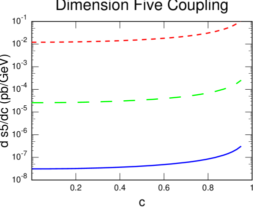
Figure 5: The differential cross section for $e^{+}e^{-}\to\gamma+GP$, against photon scattering angle in the CM frame, arising due to the dimension-five couplings of Eq. (2.6). The plot assumes an initial electron energy $E_{e}=100$ GeV, a minimum photon transverse energy $\omega_{\scriptscriptstyle T}\geq 10$ GeV, and $M_{s}=1000$ GeV. The solid line uses $n=6$, the long-dashed line $n=4$ and the short-dashed line $n=2$.

4 Bounds from Supernovae

In the previous section, we saw that the process $f\overline{f}\to\gamma V$ can be used in future experiments to set limits on the gravity scale, $M_{s}$. The exact bound obtained will depend on the number of extra dimensions $n$.

Supernovae have the potential to probe much larger values of $M_{s}$, because both gravitons and graviphotons can be emitted freely, thereby increasing the rate of energy loss. Indeed, the fact that the observed neutrino flux from the supernova SN 1987A agrees with the predictions of stellar collapse models has been used to constrain graviton emission. The authors of Ref. [11] give the following expressions for the rate of energy loss, ${\dot{\epsilon}}$, due to graviton emission:

$${\dot{\epsilon}}=\cases{5.1\times 10^{17}~{}{\hbox{erg g${}^{-1}$ s${}^{-1}$}}~{}T_{\rm MeV}^{5.5}\,M_{\rm TeV}^{-4}~{},&$n=2$ ~{},\cr 2.8\times 10^{12}~{}{\hbox{erg g${}^{-1}$ s${}^{-1}$}}~{}T_{\rm MeV}^{6.5}\,M_{\rm TeV}^{-5}~{},&$n=3$ ~{},\cr 1.7\times 10^{7}~{}{\hbox{erg g${}^{-1}$ s${}^{-1}$}}~{}T_{\rm MeV}^{7.5}\,M_{\rm TeV}^{-6}~{},&$n=4$ ~{},\cr}$$ (4.1)

where $T_{\rm MeV}=T/(1~{}{\rm MeV})$ and $M_{\rm TeV}=M_{s}/(1~{}{\rm TeV})$. Taking $T=30$ MeV, and requiring that ${\dot{\epsilon}}<10^{19}~{}{\hbox{erg g${}^{-1}$ s${}^{-1}$}}$ [12], one obtains a very stringent constraint for $n=2$: $M_{s}\mathrel{\raise 1.29167pt\hbox{$>$\kern-7.5pt\lower 4.30554pt\hbox{$\sim$}}}50$ TeV. For larger values of $n$ this constraint is weaker: $M\mathrel{\raise 1.29167pt\hbox{$>$\kern-7.5pt\lower 4.30554pt\hbox{$\sim$}}}4$ TeV (1 TeV) for $n=3$ ($n=4$). The conclusion is therefore that TeV-scale quantum gravity is possible only for $n\geq 3$.

An analogous analysis can be done for graviphoton emission. An examination of Eqs. (3.1) and (3.4) reveals that the emission of a graviphoton with dimension-5 couplings is very similar to that of a graviton, and we thus expect similar constraints. However, we see from Eq. (3.1) that the cross section for the production of a graviphoton with dimension-4 couplings is enhanced relative to graviton emission by a factor $M_{s}^{2}/s$. Since the temperature in the core of supernovae is about $30$ MeV, this enhancement factor is enormous, and this has profound implications for models with graviphotons. To estimate the energy loss for the emission of a graviphoton with dimension-4 couplings, we naively scale the graviton results up by a factor $M_{s}^{2}/s$. This yields

$${\dot{\epsilon}}=\cases{5.1\times 10^{29}~{}{\hbox{erg g${}^{-1}$ s${}^{-1}$}}~{}T_{\rm MeV}^{3.5}\,M_{\rm TeV}^{-2}&$n=2$ ~{},\cr 2.8\times 10^{24}~{}{\hbox{erg g${}^{-1}$ s${}^{-1}$}}~{}T_{\rm MeV}^{4.5}\,M_{\rm TeV}^{-3}&$n=3$ ~{},\cr 1.7\times 10^{19}~{}{\hbox{erg g${}^{-1}$ s${}^{-1}$}}~{}T_{\rm MeV}^{5.5}\,M_{\rm TeV}^{-4}&$n=4$ ~{},\cr\sim 10^{14}~{}{\hbox{erg g${}^{-1}$ s${}^{-1}$}}~{}T_{\rm MeV}^{6.5}\,M_{\rm TeV}^{-5}&$n=5$ ~{},\cr\sim 10^{9}~{}{\hbox{erg g${}^{-1}$ s${}^{-1}$}}~{}T_{\rm MeV}^{7.5}\,M_{\rm TeV}^{-6}&$n=6$ ~{}.\cr}$$ (4.2)

The expression for the energy loss for $n=5$ has been estimated by multiplying the $n=4$ formula by a simple scale factor $\sim 10^{-5}$, and similarly for $n=6$. The constraints on the gravity scale, $M_{s}$, are now considerably more stringent:

$$M_{s}\mathrel{\raise 1.29167pt\hbox{$>$\kern-7.5pt\lower 4.30554pt\hbox{$\sim$}}}\cases{10^{8}~{}{\rm TeV}~{},&$n=2$ ~{},\cr 10^{4}~{}{\rm TeV}~{},&$n=3$ ~{},\cr 10^{2}~{}{\rm TeV}~{},&$n=4$ ~{},\cr 10~{}{\rm TeV}~{},&$n=5$ ~{},\cr 1~{}{\rm TeV}~{},&$n=6$ ~{}.\cr}$$ (4.3)

Thus, allowing for a factor of 10 leeway in our naive estimates, we conclude that, for models with graviphotons with dimension-4 couplings, TeV-scale quantum gravity requires a large number of large extra dimensions, $n\geq 5$. Conversely, if there are only a small number of large extra dimensions, they cannot be large enough to be detectable at future colliders.

A comparison of graviphoton and axion emission from supernovae shows that these results are not unexpected. Since the axion has a derivative coupling to matter, the cross section for axion emission is proportional to $f_{a}^{-2}$, where $f_{a}$ is the axion decay constant. Constraints on axion emission from supernovae imply that $f_{a}\mathrel{\raise 1.29167pt\hbox{$>$\kern-7.5pt\lower 4.30554pt\hbox{$\sim$}}}10^{10}$ GeV [13]. For $n=2$, the rate for graviphoton emission is also proportional to $M_{s}^{-2}$ [see Eq. (4.2)]. Thus, purely on dimensional grounds, we expect that $M_{s}\mathrel{\raise 1.29167pt\hbox{$>$\kern-7.5pt\lower 4.30554pt\hbox{$\sim$}}}10^{10}$ GeV, and this is indeed what is found (to within a factor of 10).

Of course, implicit in the above analysis is the assumption that the dimension-4 couplings are nonzero. Indeed, we have taken the couplings $g_{f},g_{5f}$ to be a number of $O(1)$ multiplied by $M_{s}^{-n/2}$. One might therefore try to evade the above constraints by simply assuming that these couplings vanish. However, this is, in general, not possible. As discussed in Sec. 2.3.1, even if the ordinary fermions are neutral under the graviphoton $U(1)$ gauge group, dimension-4 couplings of the graviphoton to ordinary matter will be “grown” at loop level (e.g. due to mixing of the graviphoton and the $B_{\mu}$ gauge boson). Thus, although one cannot take $g_{f},g_{5f}$ to be zero, it is conceivable that they might be small, i.e. of loop-level size, $10^{-2}$, multiplied by $M_{s}^{-n/2}$. In this case, the rate for energy loss due to graviphoton emission in Eq. (4.2) would be reduced by a factor $\sim 10^{-4}$. This leads to somewhat weaker constraints on the gravity scale:

$$M_{s}\mathrel{\raise 1.29167pt\hbox{$>$\kern-7.5pt\lower 4.30554pt\hbox{$\sim$}}}\cases{10^{6}~{}{\rm TeV}~{},&$n=2$ ~{},\cr 500~{}{\rm TeV}~{},&$n=3$ ~{},\cr 10~{}{\rm TeV}~{},&$n=4$ ~{},\cr 1~{}{\rm TeV}~{},&$n=5$ ~{}.\cr}$$ (4.4)

We therefore conclude that, due to supernovae constraints on graviphoton emission, TeV-scale quantum gravity is generically possible only if there are at least four large extra dimensions. Alternatively, any explicit model of underlying brane dynamics which wishes to describe TeV-scale branes with few extra dimensions (and so to have large signals in future colliders) must be designed to insulate any of the graviphotons from ordinary matter at much better than the one-loop level.

Note that these conclusions (i) assume that the dimension-4 graviphoton couplings are as small as they can be, $g\sim 10^{-2}M_{s}^{-n/2}$, and (ii) allow for a factor of 10 error in our estimates of the supernova bound. They also assume the existence of only one light graviphoton, whereas models with many extra dimensions are likely to have many such graviphotons due to the larger number of bulk-space supersymmetries they involve, seen from the four-dimensional perspective. Our conclusions may thus be considered to be reasonably conservative.

5 Implications for Fermion-Antifermion Scattering

We next turn to potential observable effects in fermion-antifermion collisions due to graviphoton exchange, induced by the effective couplings of Eqs. (2.3) and (2.6). We find that graviphoton exchange can significantly change what would be expected from graviton exchange.

Unfortunately, this difference between graviton and graviphoton exhange is of less practical interest than was the difference found in the previous section for graviphoton and graviton production. The argument is the following. In TeV-scale quantum gravity models, graviton exchange can significantly affect fermion-antifermion scattering. This has generated a great deal of excitement, and such graviton-exchange contributions have been extensively discussed in the literature [5]. The reason that such keen interest was generated is that these effects were thought to be clean, model-independent tests for the presence of large extra dimensions. Unfortunately, this is not the case. As discussed in Ref. [6], graviton exchange is indistinguishable at low energies from other, equally large, scattering contributions due to the exchange of states having masses $M_{s}$, such as higher string modes in both the brane and bulk sectors. These other contributions are dangerous because they can contribute to fermion scattering at the same order in $1/M_{s}$ as can the graviton KK modes, and their effects depend on the details of the microscopic spectrum of the underlying theory. Thus, all the calculations in Ref. [5] are incomplete since they neglect these other, model-dependent contributions.

Obviously, this also applies to graviphotons. Although it is possible to calculate the effects of graviphoton exchange on fermion-antifermion scattering, even including the interference with graviton exchange, such calculations will also be incomplete. Even so, we present here the results for tree-level graviphoton exchange in fermion-antifermion scattering. We do so partly for the sake of completeness, and partly because these expressions are the necessary first step towards any future understanding of how to disentangle the various kinds of extra-dimensional effects.

Figure 6: The Feynman graphs giving the graviphoton-exchange contribution to fermion-antifermion scattering. As in Fig. (1), the graviphoton-fermion interaction here is a sum of the dimension-four helicity-preserving interaction of Eq. (2.3) and the dimension-five helicity-flipping interaction of Eq. (2.6).

5.1 Cross Section Formulae

The Feynman graphs which are potentially relevant for tree-level graviphoton contributions to fermion-antifermion scattering are those of Fig. (6). Again, the graviphoton-fermion coupling is the sum of the helicity-preserving dimension-four terms of Eq. (2.3) and the helicity-flipping dimension-five terms of Eq. (2.6).

In the (excellent) approximation where fermion masses are neglected, it is instructive to distinguish the cross sections for the sixteen different combinations of helicities for the fermions in the initial and final states. This is because only a limited number of couplings contribute to any one helicity combination, potentially providing a wealth of diagnostic information as to the kind of scattering which is responsible for the observed cross section.

The results are most conveniently displayed in the following way. Since fermion masses are neglected, the unpolarized cross section is $\frac{1}{4}$ the sum of the result for each possible choice of initial and final helicity. We list each of these polarized cross sections:

$${d\sigma\over du\,dt}(f_{i}\overline{f}_{j}\to g_{i^{\prime}}\overline{g}_{j^{\prime}})={1\over 4\pi\,s^{2}}\;\left|{\cal A}_{ij;i^{\prime}j^{\prime}}\right|^{2}\;\delta(s+t+u),$$ (5.1)

where $i,j,i^{\prime},j^{\prime}=L,R$ denote the helicities of the initial and final fermions. The remainder of this section gives the relevant amplitudes, ${\cal A}_{ij;i^{\prime}j^{\prime}}$, first for the case $g\neq f$ (e.g. for $e^{+}e^{-}\to\mu^{+}\mu^{-}$) and then for $g=f$ (for $e^{+}e^{-}\to e^{+}e^{-}$).

5.1.1 $e^{+}e^{-}\to\ell^{+}\ell^{-}$

Consider first the case where the final and initial fermions are distinguishable. The amplitudes relevant for this case are summarized as a function of the initial and final helicities in Table (1).

	$\ell^{-}_{\scriptscriptstyle L}\ell^{+}_{\scriptscriptstyle L}$	$\ell^{-}_{\scriptscriptstyle L}\ell^{+}_{\scriptscriptstyle R}$	$\ell^{-}_{\scriptscriptstyle R}\ell^{+}_{\scriptscriptstyle L}$	$\ell^{-}_{\scriptscriptstyle R}\ell^{+}_{\scriptscriptstyle R}$
$e^{-}_{\scriptscriptstyle L}e^{+}_{\scriptscriptstyle L}$	$|{\cal A}(\hbox{FF})|^{2}$	$|{\cal A}(\hbox{FP})|^{2}$	$|{\cal A}(\hbox{FP})|^{2}$	$|{\cal A}(\hbox{FF})|^{2}$
$e^{-}_{\scriptscriptstyle L}e^{+}_{\scriptscriptstyle R}$	$|{\cal A}(\hbox{PF})|^{2}$	$|{\cal A}_{{\scriptscriptstyle L}{\scriptscriptstyle L}}(\hbox{PP})|^{2}$	$|{\cal A}_{{\scriptscriptstyle L}{\scriptscriptstyle R}}(\hbox{PP})|^{2}$	$|{\cal A}(\hbox{PF})|^{2}$
$e^{-}_{\scriptscriptstyle R}e^{+}_{\scriptscriptstyle L}$	$|{\cal A}(\hbox{PF})|^{2}$	$|{\cal A}_{{\scriptscriptstyle R}{\scriptscriptstyle L}}(\hbox{PP})|^{2}$	$|{\cal A}_{{\scriptscriptstyle R}{\scriptscriptstyle R}}(\hbox{PP})|^{2}$	$|{\cal A}(\hbox{PF})|^{2}$
$e^{-}_{\scriptscriptstyle R}e^{+}_{\scriptscriptstyle R}$	$|{\cal A}(\hbox{FF})|^{2}$	$|{\cal A}(\hbox{FP})|^{2}$	$|{\cal A}(\hbox{FP})|^{2}$	$|{\cal A}(\hbox{FF})|^{2}$

Table 1: The amplitude, ${\cal A}$, appearing in the differential cross section, Eq. (5.1), for $e^{+}e^{-}\to\ell^{+}\ell^{-}$, for $\ell\neq e$, in the limit where electron and final-state lepton masses are neglected. The labels ‘F’ and ‘P’ are meant to indicate helicity-flipping or helicity-preserving interactions.

The functions which appear in these tables are given explicitly by:

$$|{\cal A}(\hbox{FF})|^{2} = \frac{1}{4}\,(a_{e}^{2}+b_{e}^{2})\,(a_{\mu}^{2}+b_{\mu}^{2})\;s^{2}\,(t-u)^{2}\;|F|^{2}$$ (5.2)

$$|{\cal A}(\hbox{PF})|^{2} = (a_{\mu}^{2}+b_{\mu}^{2})\,(g_{e}^{2}+g_{5e}^{2})\;s\,t\,u\;|F|^{2}$$ (5.3)

$$|{\cal A}(\hbox{FP})|^{2} = (a_{e}^{2}+b_{e}^{2})\,(g_{\mu}^{2}+g_{5\mu}^{2})\;s\,t\,u\;|F|^{2}$$ (5.4)

and

$$|{\cal A}_{{\scriptscriptstyle L}{\scriptscriptstyle L}}(\hbox{PP})|^{2} = u^{2}\,\left|\left[{e^{2}\over s}+\left({e\over s_{w}c_{w}}\right)^{2}\;{h_{e{\scriptscriptstyle L}}\,h_{\mu{\scriptscriptstyle L}}\over s-M_{\scriptscriptstyle Z}^{2}}\right]+g_{e{\scriptscriptstyle L}}\,g_{\mu{\scriptscriptstyle L}}\,F+2\kappa^{2}\;(4u+3s)\;F\right|^{2}$$ (5.5)

$$|{\cal A}_{{\scriptscriptstyle R}{\scriptscriptstyle R}}(\hbox{PP})|^{2} = u^{2}\,\left|\left[{e^{2}\over s}+\left({e\over s_{w}c_{w}}\right)^{2}\;{h_{e{\scriptscriptstyle R}}\,h_{\mu{\scriptscriptstyle R}}\over s-M_{\scriptscriptstyle Z}^{2}}\right]+g_{e{\scriptscriptstyle R}}\,g_{\mu{\scriptscriptstyle R}}\,F+2\kappa^{2}\;(4u+3s)\;F\right|^{2}$$ (5.6)

$$|{\cal A}_{{\scriptscriptstyle L}{\scriptscriptstyle R}}(\hbox{PP})|^{2} = t^{2}\,\left|\left[{e^{2}\over s}+\left({e\over s_{w}c_{w}}\right)^{2}\;{h_{e{\scriptscriptstyle L}}\,h_{\mu{\scriptscriptstyle R}}\over s-M_{\scriptscriptstyle Z}^{2}}\right]+g_{e{\scriptscriptstyle L}}\,g_{\mu{\scriptscriptstyle R}}\,F+2\kappa^{2}\;(4u+s)\;F\right|^{2}$$ (5.7)

$$|{\cal A}_{{\scriptscriptstyle R}{\scriptscriptstyle L}}(\hbox{PP})|^{2} = t^{2}\,\left|\left[{e^{2}\over s}+\left({e\over s_{w}c_{w}}\right)^{2}\;{h_{e{\scriptscriptstyle R}}\,h_{\mu{\scriptscriptstyle L}}\over s-M_{\scriptscriptstyle Z}^{2}}\right]+g_{e{\scriptscriptstyle R}}\,g_{\mu{\scriptscriptstyle L}}\,F+2\kappa^{2}\;(4u+s)\;F\right|^{2}$$ (5.8)

where $h_{\scriptscriptstyle L}=-\frac{1}{2}+s_{w}^{2}$ and $h_{\scriptscriptstyle R}=s_{w}^{2}$ denote the couplings of left- and right-handed fermions to the $Z$ boson, while $g_{\scriptscriptstyle L}=(g+g_{5})$ and $g_{\scriptscriptstyle R}=(g-g_{5})$ are the corresponding dimension-four fermion couplings to the graviphoton. All of these expressions neglect the mass of the initial and final state fermions, as well as the $(4+n)$-dimensional mass, $m_{\scriptscriptstyle V}$, of the graviphoton.

The quantity $F$ in these expressions is the function defined by:

$$F(s)=\int{d^{n}Q\over(2\pi)^{n}}\;{1\over Q^{2}-s},$$ (5.9)

and so $F\to-1/s$ as $n\to 0$ – i.e. in the absence of extra dimensions. Since this expression diverges in the ultraviolet, for $n\geq 2$, we follow the practice in the literature and take it to be cut off at the scale $Q^{2}=M_{s}^{2}$, making $F$ approximately constant ($F=\Omega_{n}M_{s}^{n-2}/[(n-2)(2\pi)^{n}]$ if $n>2$, up to $O(s/M_{s}^{2})$ corrections). Because the couplings $g,g_{5}$ and $\kappa$ are the higher-dimensional ones, this form for $F$ implies

$$g^{2}F\sim{1\over M_{s}^{2}}\qquad\hbox{and}\qquad a^{2}F\sim\kappa^{2}F\sim{1\over M_{s}^{4}},$$ (5.10)

and so the four-dimensional Planck scale, $M_{p}$, drops out of these expressions in the usual way. (From the four-dimensional point of view it does so because the factor of $1/M_{p}$ in the coupling cancels factors of $M_{p}$ in the density of states of the KK modes.)

Notice that the necessity to cut off the integral in Eq. (5.9) is a symptom that the graviphoton and graviton contributions are competing with the low-energy effects of exchanging heavier (string) states having masses of order $M_{s}$. These two issues are connected because the ultraviolet divergence we are regulating must be absorbable into the renormalization of an effective coupling of the low-energy theory. (Such a renormalization is indeed possible because the relevant terms in Eqs. (5.2) through (5.8) are polynomials in $s,t$ and $u$, and so correspond to the effects of local operators.) The couplings whose renormalizations do the job are precisely those of the effective interactions which are generated on integrating out the mass-$M_{s}$ heavy states.

Figure 7: The Feynman graphs giving the graviphoton-exchange contribution to fermion-antifermion scattering, when the initial and final fermions are indistinguishable. As for previous figures, the graviphoton-fermion interaction here is a sum of the dimension-four helicity-preserving interaction of Eq. (2.3) and the dimension-five helicity-flipping interaction of Eq. (2.6).

5.1.2 $e^{+}e^{-}\to e^{+}e^{-}$

Next consider the corresponding expressions for the case where initial and final particles are indistinguishable, $f=g$ (and so which apply for $e^{+}e^{-}\to e^{+}e^{-}$). The Feynman graphs relevant to this process are given in Fig. (7), and differ from the previous case by the inclusion of $t$-channel graphs. Neglecting the electron mass gives the total cross section as $\frac{1}{4}$ the sum over the polarized cross sections, which we again express as in Eq. (5.1). The results for the polarized cross sections obtained from evaluating the graphs of Fig. (7) are listed in Table (2).

	$e^{-}_{\scriptscriptstyle L}e^{+}_{\scriptscriptstyle L}$	$e^{-}_{\scriptscriptstyle L}e^{+}_{\scriptscriptstyle R}$	$e^{-}_{\scriptscriptstyle R}e^{+}_{\scriptscriptstyle L}$	$e^{-}_{\scriptscriptstyle R}e^{+}_{\scriptscriptstyle R}$
$e^{-}_{\scriptscriptstyle L}e^{+}_{\scriptscriptstyle L}$	$|{\cal A}_{{\scriptscriptstyle L}{\scriptscriptstyle R}}^{{\scriptscriptstyle F}{\scriptscriptstyle F}}(s)+{\cal A}_{{\scriptscriptstyle L}{\scriptscriptstyle R}}^{{\scriptscriptstyle P}{\scriptscriptstyle P}}(t)|^{2}$	$|{\cal A}_{{\scriptscriptstyle L}{\scriptscriptstyle L}}^{{\scriptscriptstyle F}{\scriptscriptstyle P}}(s)+{\cal A}_{{\scriptscriptstyle L}{\scriptscriptstyle L}}^{{\scriptscriptstyle P}{\scriptscriptstyle F}}(t)|^{2}$	$|{\cal A}_{{\scriptscriptstyle L}{\scriptscriptstyle R}}^{{\scriptscriptstyle F}{\scriptscriptstyle P}}(s)+{\cal A}_{{\scriptscriptstyle L}{\scriptscriptstyle R}}^{{\scriptscriptstyle F}{\scriptscriptstyle P}}(t)|^{2}$	$|{\cal A}_{{\scriptscriptstyle L}{\scriptscriptstyle L}}^{{\scriptscriptstyle F}{\scriptscriptstyle F}}(s)+{\cal A}_{{\scriptscriptstyle L}{\scriptscriptstyle L}}^{{\scriptscriptstyle F}{\scriptscriptstyle F}}(t)|^{2}$
$e^{-}_{\scriptscriptstyle L}e^{+}_{\scriptscriptstyle R}$	$|{\cal A}_{{\scriptscriptstyle L}{\scriptscriptstyle R}}^{{\scriptscriptstyle P}{\scriptscriptstyle F}}(s)+{\cal A}_{{\scriptscriptstyle L}{\scriptscriptstyle R}}^{{\scriptscriptstyle P}{\scriptscriptstyle F}}(t)|^{2}$	$|{\cal A}_{{\scriptscriptstyle L}{\scriptscriptstyle L}}^{{\scriptscriptstyle P}{\scriptscriptstyle P}}(s)+{\cal A}_{{\scriptscriptstyle L}{\scriptscriptstyle L}}^{{\scriptscriptstyle P}{\scriptscriptstyle P}}(t)|^{2}$	$|{\cal A}_{{\scriptscriptstyle L}{\scriptscriptstyle R}}^{{\scriptscriptstyle P}{\scriptscriptstyle P}}(s)+{\cal A}_{{\scriptscriptstyle L}{\scriptscriptstyle R}}^{{\scriptscriptstyle F}{\scriptscriptstyle F}}(t)|^{2}$	$|{\cal A}_{{\scriptscriptstyle L}{\scriptscriptstyle L}}^{{\scriptscriptstyle P}{\scriptscriptstyle F}}(s)+{\cal A}_{{\scriptscriptstyle L}{\scriptscriptstyle L}}^{{\scriptscriptstyle F}{\scriptscriptstyle P}}(t)|^{2}$
$e^{-}_{\scriptscriptstyle R}e^{+}_{\scriptscriptstyle L}$	$|{\cal A}_{{\scriptscriptstyle R}{\scriptscriptstyle R}}^{{\scriptscriptstyle P}{\scriptscriptstyle F}}(s)+{\cal A}_{{\scriptscriptstyle R}{\scriptscriptstyle R}}^{{\scriptscriptstyle F}{\scriptscriptstyle P}}(t)|^{2}$	$|{\cal A}_{{\scriptscriptstyle R}{\scriptscriptstyle L}}^{{\scriptscriptstyle P}{\scriptscriptstyle P}}(s)+{\cal A}_{{\scriptscriptstyle R}{\scriptscriptstyle L}}^{{\scriptscriptstyle F}{\scriptscriptstyle F}}(t)|^{2}$	$|{\cal A}_{{\scriptscriptstyle R}{\scriptscriptstyle R}}^{{\scriptscriptstyle P}{\scriptscriptstyle P}}(s)+{\cal A}_{{\scriptscriptstyle R}{\scriptscriptstyle R}}^{{\scriptscriptstyle P}{\scriptscriptstyle P}}(t)|^{2}$	$|{\cal A}_{{\scriptscriptstyle R}{\scriptscriptstyle L}}^{{\scriptscriptstyle P}{\scriptscriptstyle F}}(s)+{\cal A}_{{\scriptscriptstyle R}{\scriptscriptstyle L}}^{{\scriptscriptstyle P}{\scriptscriptstyle F}}(t)|^{2}$
$e^{-}_{\scriptscriptstyle R}e^{+}_{\scriptscriptstyle R}$	$|{\cal A}_{{\scriptscriptstyle R}{\scriptscriptstyle R}}^{{\scriptscriptstyle F}{\scriptscriptstyle F}}(s)+{\cal A}_{{\scriptscriptstyle R}{\scriptscriptstyle R}}^{{\scriptscriptstyle F}{\scriptscriptstyle F}}(t)|^{2}$	$|{\cal A}_{{\scriptscriptstyle R}{\scriptscriptstyle L}}^{{\scriptscriptstyle F}{\scriptscriptstyle P}}(s)+{\cal A}_{{\scriptscriptstyle R}{\scriptscriptstyle L}}^{{\scriptscriptstyle F}{\scriptscriptstyle P}}(t)|^{2}$	$|{\cal A}_{{\scriptscriptstyle R}{\scriptscriptstyle R}}^{{\scriptscriptstyle F}{\scriptscriptstyle P}}(s)+{\cal A}_{{\scriptscriptstyle R}{\scriptscriptstyle R}}^{{\scriptscriptstyle P}{\scriptscriptstyle F}}(t)|^{2}$	$|{\cal A}_{{\scriptscriptstyle R}{\scriptscriptstyle L}}^{{\scriptscriptstyle F}{\scriptscriptstyle F}}(s)+{\cal A}_{{\scriptscriptstyle R}{\scriptscriptstyle L}}^{{\scriptscriptstyle P}{\scriptscriptstyle P}}(t)|^{2}$

Table 2: The amplitude, ${\cal A}$, appearing in the differential cross section, Eq. (5.1), for $e^{+}e^{-}\to e^{+}e^{-}$, in the limit where electron mass is neglected. The labels ‘F’ and ‘P’ are meant to indicate helicity-flipping or helicity-preserving interactions, and ‘$s$’ and ‘$t$’ indicate the results of $s$- and $t$-channel graphs.

The $s$-channel amplitudes which appear in this table are given by the following expressions (when the graviphoton and electron masses are neglected).

$${\cal A}_{{\scriptscriptstyle L}{\scriptscriptstyle L}}^{{\scriptscriptstyle F}{\scriptscriptstyle F}}(s)=\Bigl{(}{\cal A}_{{\scriptscriptstyle R}{\scriptscriptstyle R}}^{{\scriptscriptstyle F}{\scriptscriptstyle F}}(s)\Bigr{)}^{*} = \frac{1}{2}\,(a_{e}+ib_{e})^{2}\;s\,(t-u)\;F(s)$$

$${\cal A}_{{\scriptscriptstyle L}{\scriptscriptstyle R}}^{{\scriptscriptstyle F}{\scriptscriptstyle F}}(s)={\cal A}_{{\scriptscriptstyle R}{\scriptscriptstyle L}}^{{\scriptscriptstyle F}{\scriptscriptstyle F}}(s) = \frac{1}{2}\,\Bigl{(}a_{e}^{2}+b_{e}^{2}\Bigr{)}\;s\,(t-u)\;F(s),$$ (5.11)

$${\cal A}_{{\scriptscriptstyle L}{\scriptscriptstyle L}}^{{\scriptscriptstyle F}{\scriptscriptstyle P}}(s)={\cal A}_{{\scriptscriptstyle L}{\scriptscriptstyle L}}^{{\scriptscriptstyle P}{\scriptscriptstyle F}}(s)=\Bigl{(}{\cal A}_{{\scriptscriptstyle L}{\scriptscriptstyle R}}^{{\scriptscriptstyle P}{\scriptscriptstyle F}}(s)\Bigr{)}^{*}=\Bigl{(}{\cal A}_{{\scriptscriptstyle R}{\scriptscriptstyle L}}^{{\scriptscriptstyle F}{\scriptscriptstyle P}}(s)\Bigr{)}^{*} = g_{e{\scriptscriptstyle L}}\,(a_{e}+ib_{e})\,\sqrt{stu}\;F(s)$$

$${\cal A}_{{\scriptscriptstyle L}{\scriptscriptstyle R}}^{{\scriptscriptstyle F}{\scriptscriptstyle P}}(s)={\cal A}_{{\scriptscriptstyle R}{\scriptscriptstyle L}}^{{\scriptscriptstyle P}{\scriptscriptstyle F}}(s)=\Bigl{(}{\cal A}_{{\scriptscriptstyle R}{\scriptscriptstyle R}}^{{\scriptscriptstyle P}{\scriptscriptstyle F}}(s)\Bigr{)}^{*}=\Bigl{(}{\cal A}_{{\scriptscriptstyle R}{\scriptscriptstyle R}}^{{\scriptscriptstyle F}{\scriptscriptstyle P}}(s)\Bigr{)}^{*} = g_{e{\scriptscriptstyle R}}\,(a_{e}+ib_{e})\,\sqrt{stu}\;F(s)$$

and

$${\cal A}_{{\scriptscriptstyle L}{\scriptscriptstyle L}}^{{\scriptscriptstyle P}{\scriptscriptstyle P}}(s) = u\,\left\{\left[{e^{2}\over s}+\left({e\over s_{w}c_{w}}\right)^{2}\;{h_{e{\scriptscriptstyle L}}^{2}\over s-M_{\scriptscriptstyle Z}^{2}}\right]+\left[g_{e{\scriptscriptstyle L}}^{2}+2\kappa^{2}\;(4u+3s)\right]F(s)\right\}$$

$${\cal A}_{{\scriptscriptstyle R}{\scriptscriptstyle R}}^{{\scriptscriptstyle P}{\scriptscriptstyle P}}(s) = u\,\left\{\left[{e^{2}\over s}+\left({e\over s_{w}c_{w}}\right)^{2}\;{h_{e{\scriptscriptstyle R}}^{2}\over s-M_{\scriptscriptstyle Z}^{2}}\right]+\left[g_{e{\scriptscriptstyle R}}^{2}+2\kappa^{2}\;(4u+3s)\right]F(s)\right\}$$ (5.13)

$${\cal A}_{{\scriptscriptstyle L}{\scriptscriptstyle R}}^{{\scriptscriptstyle P}{\scriptscriptstyle P}}(s)={\cal A}_{{\scriptscriptstyle R}{\scriptscriptstyle L}}^{{\scriptscriptstyle P}{\scriptscriptstyle P}}(s) = t\,\left\{\left[{e^{2}\over s}+\left({e\over s_{w}c_{w}}\right)^{2}\;{h_{e{\scriptscriptstyle L}}\,h_{e{\scriptscriptstyle R}}\over s-M_{\scriptscriptstyle Z}^{2}}\right]+\left[g_{e{\scriptscriptstyle L}}\,g_{e{\scriptscriptstyle R}}+2\kappa^{2}\;(4u+s)\right]F(s)\right\}$$

The $t$-channel amplitudes are obtained from these through the replacement $(s,t,u)\to(t,s,u)$.

5.2 Discussion

The cross sections for graviphoton-exchange processes share many features which are similar to those shown by the graviphoton production cross sections. In particular, those interactions involving the nonderivative (dimension-four) couplings can dominate both graviphoton exchange through the magnetic-moment interaction and graviton exchange. It can so dominate for two reasons:

1. Since the nonderivative interaction involves fewer derivatives, it is less suppressed by powers of $s/M_{s}^{2}$ than are the others.

2. Since it has the same helicity properties as have the Standard-Model photon and $Z$ couplings, it – like the graviton but unlike the magnetic moment interaction – can interfere with the Standard-Model amplitudes, and so contribute linearly in the cross section.

Despite this relative enhancement, even tree-level dimension-four graviphoton couplings cannot yet be ruled out by accelerator experiments. This is because, even at the $Z$ peak, $Z$-graviphoton interference gives corrections which are of order $M_{\scriptscriptstyle Z}^{2}/M_{s}^{2}\mathrel{\raise 1.29167pt\hbox{$<$\kern-7.5pt\lower 4.30554pt\hbox{$\sim$}}}1\%$ so long as $M_{s}\mathrel{\raise 1.29167pt\hbox{$>$\kern-7.5pt\lower 4.30554pt\hbox{$\sim$}}}1$ TeV.

6 Summary and Discussion

There has been a great deal of interest in the possibility that extra spatial dimensions could be quite large, and that the scale of quantum gravity could be as low as about a TeV. Although supersymmetry is not a prerequisite for such a scenario, it is nevertheless true that its most realistic framework, M theory, does possess supersymmetry. In this paper, we have examined the consequences of supersymmetry for low-scale quantum gravity.

Since the graviton lives in a higher-dimensional space, it is represented by a supermultiplet for a higher-dimensional supersymmetry. In four dimensions, this supermultiplet includes several particles, including (at least) one spin-one boson, the graviphoton. Furthermore, because the graviphoton is related to the graviton by supersymmetry, and since its couplings are gravitational in strength, its mass is of order $M_{s}^{2}/M_{p}$, where $M_{s}$ is the scale of supersymmetry breaking and $M_{p}$ is the four-dimensional Planck mass. Therefore, just as the graviton can be represented in four dimensions as a tower of Kaluza-Klein states, so can the graviphoton, with the principal difference being that, while the lowest-mass graviton state has $m=0$, the lowest-mass graviphoton state has $m=M_{s}^{2}/M_{p}\sim 10^{-3}$ eV for $M_{s}\sim 1$ TeV. The presence of the graviphoton can have important effects on the experimental signatures for low-scale quantum gravity.

We must stress that, while various aspects of supersymmetry are model-dependent (e.g. the number of supersymmetries, whether or not they are broken on the brane, etc.), the existence of the graviphoton is not. Thus, any supersymmetric model of TeV-scale quantum gravity must take into account the effects due to the presence of the graviphoton, in particular the constraints on graviphoton emission.

We consider two possibilities for the coupling of the graviphoton to ordinary matter. First, the coupling can take the form of a dimension-5 magnetic-moment term. In this case, purely on dimensonal grounds, one expect rates for processes involving graviphotons to be of the same order as those involving gravitons. After all, for a graviphoton dimension-5 coupling to matter, both the graviton and graviphoton are derivatively coupled, and the coupling constants for both particles have the same dimensions.

The second, more interesting possibility is that the graviphoton can couple to ordinary matter via dimension-4 vector and/or axial-vector interactions. This can arise if ordinary matter has nonzero charges under the $U(1)$ group gauged by graviphotons. More importantly, even if those charges are zero, dimension-4 graviphoton couplings will be generated, in general, by the mixing of the graviphoton with the neutral standard-model gauge bosons. Since this kind of mixing does not decouple, it will happen so long as any states carry both graviphoton and ordinary Standard-Model charges, regardless of how massive these states might be. Therefore, we expect, on quite general grounds, that the dimension-4 graviphoton couplings are at least of loop size, and may be larger.

Once these dimension-4 couplings are generated, there are very stringent constraints on the number of large extra dimensions and/or the scale of quantum gravity, $M_{s}$. The point is the following. A key feature of low-scale quantum gravity is the possibility of emitting bulk-space particles (like gravitons and graviphotons) when ordinary particles collide. This process permits ordinary matter to lose energy into what are effectively invisible degrees of freedom. But the agreement between the measured rate of energy loss of the supernova SN 1987A with theoretical expectations due to neutrino emission provides a bound on the rate of energy loss into other invisible species. For gravitons it was found that this constraint permits $M_{s}\sim 1$ TeV only if the number of extra dimensions, $n$, satisfies $n>2$ [11].

If graviphotons are also present, then they will also contribute to the energy loss of supernovae. However, all processes involving gravitational particles are suppressed by powers of $E/M_{s}$, where $E$ is the energy scale of the process in question. (This is why it is possible for low-scale gravity effects to have remained undetected until now.) But should the graviphoton have a dimension-4 coupling to matter, the cross section for its emission is enhanced by a factor $(M_{s}/E)^{2}$ compared to that for graviton emission. Since the temperature inside a supernova is around 30 MeV, this enchancement factor is enormous: the rate for graviphoton emission can be larger than that for graviton emission by about $10^{12}$. This leads to considerably stronger supernova constraints on $n$ and/or $M_{s}$.

The strongest bounds arise if the dimension-4 couplings arise at tree level (i.e. the ordinary fermions have charges under the graviphoton $U(1)$). In this case we find that $M_{s}\sim 1$ TeV is permitted only for $n\geq 5$. If one assumes that the dimension-4 couplings are instead only of one-loop size, then the constraints are slightly weaker: $n\geq 4$ is required in order to have $M_{s}\sim 1$ TeV. We must stress that these are very conservative results. We have allowed for an error of a factor of 10 in our supernova estimates, and we have ignored the fact that, for larger values of $n$, the graviton supermultiplet typically contains several graviphotons, and so can have even stronger constraints.

We therefore conclude that, for models of low-scale quantum gravity which include supersymmetry, either the number of large extra dimensions is large, at least $n=4$, or there must be some symmetry which prevents the generation of low-energy dimension-4 graviphoton couplings to ordinary matter.

These constraints also affect the prospects for experimentally detecting gravitational effects at accelerators. As described above, one of the most important processes for detection is the emission of a final-state gravitational particle. However, the cross section for the process $f\overline{f}\to\gamma+GP$ is proportional to $(E/M_{s})^{n}$. Thus, for energies $E$ well below the gravity scale, larger values of $n$ lead to smaller cross sections. (That is, paradoxically, the more large extra dimensions there are, the harder it is to detect them). Note that this holds both for graviphotons (with dimension-4 and/or dimension-5 couplings) and gravitons.

This is shown explicitly in Figs. (2) through (5): we see that larger values of $n$ lead to considerably smaller cross sections. However, we also note that, should a gravitational signal be found, one might hope to distinguish between the spin-1 graviphoton and the spin-2 graviton by the angular distribution of the emitted photon.

Finally, the graviphoton can also contribute virtually to fermion-antifermion scattering. Unlike gravitational emission, this contribution is independent of the number of large extra dimensions. However, a word of caution is appropriate here: should a signal of gravitational new physics be found in the measurement of $f{\bar{f}}\to g{\bar{g}}$, it is unlikely that we will be able to identify the type of virtual state responsible. This is because, in addition to the graviton and graviphoton, higher string modes can also contribute to the scattering at the same order in $1/M_{s}$ [6].

As usual, the contributions of the graviton and graviphoton are suppressed by powers of $E/M_{s}$. The contributions of the graviphoton with dimension-5 couplings to matter are quite similar in size to those of the graviton. However, as above, the contributions of the graviphoton with dimension-4 couplings are larger than those of the graviton by a factor $M_{s}^{2}/s$ in the amplitude. Even so, it is not possible to detect the presence of a graviphoton in low-energy experiments. Even at the $Z$ peak, taking into account $Z$-graviphoton interference, gravitational correctons are at most of order $M_{Z}^{2}/M_{s}^{2}\sim 1\%$. Thus, if one hopes to detect virtual gravitational contributions, one really needs experiments where the centre-of-mass energy approaches the scale of quantum gravity.

Finally, we remark that one can learn something about the nature of the virtual contributions to fermion-antifermion scattering if one can polarize the initial fermions and measure the helicities of the final-state fermions. This can be seen by examining the graviphoton couplings. The dimension-4 couplings are helicity-preserving (as are the graviton couplings), while the dimension-5 couplings are helicity flipping. Thus a cross-section measurement as a function of helicity is a powerful diagnostic of the presence of large extra dimensions.

Acknowledgements

We thank Karim Benakli for helpful discussions. This research was supported in part by U.S. DOE contracts DE-FG02-94ER40817 (ISU), NSERC of Canada, and FCAR du Québec.

References

- [1] For reviews see, for example: J. H. Schwarz, Nucl. Phys. Proc. Suppl. 55B, 1 (1997) [hep-th/9607201]; M. J. Duff, Int. J. Mod. Phys. A11, 5623 (1996) [hep-th/9608117]; J. Polchinski, hep-th/9611050; P. K. Townsend, hep-th/9612121; C. Bachas, hep-th/9806199; C.V. Johnson, hep-th/9812196.
- [2] N. Arkani-Hamed, S. Dimopoulos and G. Dvali, Phys. Lett. B429 (1998) 263 [hep-ph/9803315]; Phys. Rev. D59 (1999) 086004 [hep-ph/9807344]; I. Antoniadis, N. Arkani-Hamed, S. Dimopoulos and G. Dvali, Phys. Lett. B436 (1998) 257 [hep-ph/9804398]; P. Horava and E. Witten, Nucl. Phys. B475 (1996) 94 [hep-th/9603142]; Nucl. Phys. B460 (1996) 506 [hep-th/9510209]; E. Witten, Nucl. Phys. B471 (1996) 135 [hep-th/9602070]; J. Lykken, Phys. Rev. D54 (1996) 3693 [hep-th/9603133]; I. Antoniadis, Phys. Lett. B246 (1990) 377.
- [3] L. Randall, R. Sundrum, Phys. Rev. Lett. 83 (1999) 3370 [hep-ph/9905221], Phys. Rev. Lett. 83 (1999) 4690 [hep-th/9906064].
- [4] Real graviton emission is discussed in G. F. Giudice, R. Rattazzi and J. D. Wells, Nucl. Phys. B544, 3 (1999) [hep-ph/9811291]; E. A. Mirabelli, M. Perelstein and M. E. Peskin, Phys. Rev. Lett. 82, 2236 (1999) [hep-ph/9811337]; T. Han, J. D. Lykken and R. Zhang, Phys. Rev. D59, 105006 (1999) [hep-ph/9811350]; K. Cheung and W.-Y. Keung, Phys. Rev. D60, 112003 (1999) [hep-ph/9903294]; S. Cullen and M. Perelstein, Phys. Rev. Lett. 83 (1999) 268 [hep-ph/9903422]; C. Balázs et al., Phys. Rev. Lett. 83 (1999) 2112 [hep-ph/9904220]; L3 Collaboration (M. Acciarri et al.), Phys. Lett. B464, 135 (1999), [hep-ex/9909019], Phys. Lett. B470, 281 (1999) [hep-ex/9910056].
- [5] There is an extensive literature examining the effects of virtual graviton exchange. For a review, along with a comprehensive list of references, see K. Cheung, talk given at the 7th International Symposium on Particles, Strings and Cosmology (PASCOS 99), Tahoe City, California, Dec 1999, hep-ph/0003306.
- [6] E. Accomando, I. Antoniadis and K. Benakli, Nucl. Phys. B579, 3 (2000) [hep-ph/9912287]; S. Cullen, M. Perelstein and M. E. Peskin, hep-ph/0001166;
- [7] See, however, G. Aldazabal, L. E. Ibanez and F. Quevedo, JHEP 0001, 031 (2000) [hep-th/9909172], hep-ph/0001083; M. Cvetic, M. Plumacher and J. Wang, JHEP 0004, 004 (2000) [hep-th/9911021].
- [8] K. R. Dienes, E. Dudas and T. Gherghetta, Nucl. Phys. B557, 25 (1999) [hep-ph/9811428]; A. E. Faraggi and M. Pospelov, Phys. Lett. B458, 237 (1999) [hep-ph/9901299]; H. Abe, H. Miguchi and T. Muta, Mod. Phys. Lett. A15, 445 (2000) [hep-ph/0002212]; R. Barbieri, P. Creminelli and A. Strumia, hep-ph/0002199; E. Ma, G. Rajasekaran and U. Sarkar, hep-ph/0006340.
- [9] F. Leblond, McGill preprint in preparation.
- [10] D. Z. Freedman, Phys. Rev. Lett. 38, 105 (1977); S. Ferrara, J. Scherk and B. Zumino, Phys. Lett. B66, 35 (1977); P. Breitenlohner and A. Kabelschacht, Nucl. Phys. B148, 96 (1979); E. S. Fradkin and M. A. Vasiliev, Phys. Lett. B85 (1979) 47; P. Breitenlohner and M. F. Sohnius, Nucl. Phys. B165, 483 (1980), Nucl. Phys. B187, 409 (1981); J. Bagger and E. Witten, Nucl. Phys. B222, 1 (1983); B. de Wit, P. G. Lauwers, R. Philippe, S. Q. Su and A. Van Proeyen, Phys. Lett. B134, 37 (1984); J. P. Derendinger, S. Ferrara, A. Masiero and A. van Proeyen, Phys. Lett. B136, 354 (1984); E. Cremmer, C. Kounnas, A. Van Proeyen, J. P. Derendinger, S. Ferrara, B. de Wit and L. Girardello, Nucl. Phys. B250, 385 (1985); P. Fre, Nucl. Phys. Proc. Suppl. 55B, 229 (1997) [hep-th/9611182].
- [11] S. Cullen and M. Perelstein, Ref. [4].
- [12] This criterion is suggested in G.G. Raffelt, Stars as Laboratories for Fundamental Physics, (University of Chicago Press, Chicago, 1996).
- [13] M. Fukugita, S. Watamura and M. Yoshimura, Phys. Rev. D26, 1840 (1982); N. Iwamoto, Phys. Rev. Lett. 53 (1984) 1198; G. G. Raffelt, Phys. Rev. D33, 897 (1986); M. S. Turner, Phys. Rept. 197, 67 (1990).