Standard Model correlations between $K\to\pi\nu\bar{\nu}$ decays and observables in $B$ Physics

Abstract

Including the recent preliminary results of BaBar and BELLE experiments, we update the currently allowed intervals for various CKM parameters: $\bar{\rho}$, $\bar{\eta}$, $\sin 2\beta$, $\sin 2\alpha$, $\sin^{2}\gamma$. We also update the SM prediction for the rates of the $K_{L}\to\pi^{0}\nu\bar{\nu}$ and $K^{+}\to\pi^{+}\nu\bar{\nu}$ decays, their ratio $a_{\pi\nu\bar{\nu}}$, as well as for certain observables related to $B$ Physics like the CP asymmetries $a_{\psi K_{S}}$ in $B^{0}_{d}\to J/\psi\,K_{S}$ and $a_{\psi\phi}$ in $B^{0}_{s}\to J/\psi\,\phi$ or the mass differences $\Delta m_{q}$ ($q=d,s$) in the $B^{0}_{q}-\bar{B}^{0}_{q}$ systems. We investigate the correlations between them. The strongest correlations are between i) $a_{\pi\nu\bar{\nu}}$ and $a_{\psi K_{S}}$, ii) $\mbox{BR}(K^{+}\to\pi^{+}\nu\bar{\nu})$ and $\Delta m_{d}/\Delta m_{s}$ and iii) $\mbox{BR}(K_{L}\to\pi^{0}\nu\bar{\nu})$ and $a_{\psi\phi}$. These correlations are likely to be violated in the presence of New Physics and therefore provide stringent tests of the Standard Model.

I Introduction

The CKM mixing matrix of the Standard Model (SM) provides a consistent explanation of all experimental data on quark flavor mixing and CP violation. Yet, some of its parameters have not been measured very accurately. It could well be that future experiments reveal inconsistencies and require contributions to flavor physics from New Physics. In particular, among the four Wolfenstein parameters $(\lambda,A,\rho,\eta)$ [1] that describe the CKM matrix [2] only two have been determined with a good accuracy [3]:

$$\lambda=0.2205\pm 0.0018~{}~{}~{}~{}~{}\mbox{and}~{}~{}~{}~{}~{}A=0.826\pm 0.041\,,$$ (1)

while the uncertainty for $(\rho,\eta)$, which describe the apex of the unitarity triangle from

$$V_{ud}V_{ub}^{*}+V_{cd}V_{cb}^{*}+V_{td}V_{tb}^{*}=0\,,$$ (2)

is rather large. As a consequence the single CP violating phase of the SM is relatively weakly determined to be:

$$\delta=\arctan(\eta/\rho)\simeq\pi/4-\pi/2\,.$$ (3)

At present the only unambiguous indication for CP violation (CPV) stems from the neutral kaon system. In particular for a long time there has been evidence for CPV in mixing from the measurement of the parameter [4]:

$$\epsilon_{K}=(2.280\pm 0.013)\times 10^{-3}\exp(i\phi_{\epsilon})\,,\,~{}~{}~{}~{}~{}\phi_{\epsilon}\simeq\pi/4\,.$$ (4)

CPV is still to be seen for other mesons, the best candidate being the observation of a CP asymmetry in $B^{0}_{d}\to J/\psi\,K_{S}$ decays, where at present $1.75\sigma$ is the combined result [5] of the three most recent related experiments, CDF BaBar and BELLE [6, 7, 8]. Another interesting signal for CPV is the $K_{L}\to\pi^{0}\nu\bar{\nu}$ decay.

The Standard Model makes definite predictions for the rates of the $K\to\pi\nu\bar{\nu}$ decays and for the observables related to $B$ physics like the mass differences $\Delta m_{q}$ ($q=d,s$) in the $B^{0}_{q}-\bar{B}^{0}_{q}$ systems and the CP asymmetries in their decays. Combinations of some of these observables, i.e. the ratios $\Gamma[K_{L}\to\pi^{0}\nu\bar{\nu}]/\Gamma[K^{+}\to\pi^{+}\nu\bar{\nu}]$ and $\Delta m_{d}/\Delta m_{s}$ have rather small uncertainties and therefore present excellent probes to test the SM. If future measurements determine any of these variables to lie outside the intervals predicted by the SM, this will be a clear evidence for New Physics. Moreover, since the SM predictions essentially depend only on the values of $\eta$ and $\rho$ there exist strong correlations between some of the observables. Then, even if each single observable is measured to be within its SM range, inconsistencies could still arise if correlations between various observables are violated.

This work is organized as follows: In section II we define the relevant set of observables and discuss their experimental status. In section III we present the SM predictions for these quantities in terms of $\rho$ and $\eta$. Our discussion contains a careful translation of the relevant CKM matrix elements into the Wolfenstein parameters including corrections of order $\lambda^{2}$ with respect to the leading order. In section IV we update the allowed region for $(\rho,\eta)$ in order to determine the present intervals for each observable within the SM. Then we consider the correlations between the various observables or their combinations. We find particularly strong correlations between i) the ratio $a_{\pi\nu\bar{\nu}}$ between the $K_{L}\to\pi^{0}\nu\bar{\nu}$ and $K^{+}\to\pi^{+}\nu\bar{\nu}$ decay rates and the CP asymmetry $a_{\psi K_{S}}$, ii) $\mbox{BR}(K^{+}\to\pi^{+}\nu\bar{\nu})$ and $\Delta m_{d}/\Delta m_{s}$ and iii) $\mbox{BR}(K_{L}\to\pi^{0}\nu\bar{\nu})$ and $a_{\psi\phi}$. We conclude in section V.

II Observables: Definitions and experimental status

A $K\to\pi\nu\bar{\nu}$ decays

The rare semi-leptonic decays $K^{+}\to\pi^{+}\nu\bar{\nu}$ and $K_{L}\to\pi^{0}\nu\bar{\nu}$ contain valuable information about the underlying physics relevant to these processes. Since these decays are expected to be dominated by short distance contributions they are subject to a rather clean theoretical interpretation.

However, due to the neutrinos in the final state the $K\to\pi\nu\bar{\nu}$ decays present an experimental challenge and so far only the branching ratio (BR) of the semi-leptonic decay $K^{+}\to\pi^{+}\nu\bar{\nu}$ has been measured with rather large uncertainty [9]

$$\mbox{BR}(K^{+}\to\pi^{+}\nu\bar{\nu})=(1.5^{+3.4}_{-1.2})\times 10^{-10}\,.$$ (5)

The detection of the $K_{L}\to\pi^{0}\nu\bar{\nu}$ decay is even more challenging: The final state has a very difficult signature since it contains no charged particles. At present we only have an upper bound on the BR [10]:

$$\mbox{BR}(K_{L}\to\pi^{0}\nu\bar{\nu})<5.9\times 10^{-7}\ \ \ (95\,\%\ \,{\rm CL})\,,$$ (6)

which lies about four order of magnitudes above the SM prediction. However, using isospin symmetry a model independent bound has been derived in Ref. [11]:

$$\mbox{BR}(K_{L}\to\pi^{0}\nu\bar{\nu})<4.4\,\mbox{BR}(K_{L}^{+}\to\pi^{+}\nu\bar{\nu})\,.$$ (7)

Then the measurement in eq. (5) implies a more restrictive upper bound:

$$\mbox{BR}(K_{L}\to\pi^{0}\nu\bar{\nu})\ \hbox to0.0pt{\raise 3.0pt\hbox{$<$}\hss}{\lower 3.0pt\hbox{$\sim$}}\ 6.6\times 10^{-10}\,.$$ (8)

Several experiments with the sensitivity to measure this BR at the SM level have been proposed: BNL-E926 at Brookhaven [12], KAMI collaboration at Fermilab [13] and KEK in Japan [14].

The knowledge of the above decay rates would also allow to determine their ratio

$$a_{\pi\nu\bar{\nu}}\equiv{\Gamma(K_{L}\to\pi^{0}\nu\bar{\nu})\over\Gamma(K^{+}\to\pi^{+}\nu\bar{\nu})}\,,$$ (9)

which is relatively clean from the theoretical point of view.

B Neutral $B$ system

The neutral $B$ system has already began to be studied with improved precision by the BaBar and BELLE experiments [7, 8] and will be further studied with unprecedented precision by the BaBar, BELLE, HERA-B, CLEO-III, CDF and D0 experiments [15]. So far the mass difference $\Delta m_{q}\equiv m(B_{q}^{H})-m(B_{q}^{L})$ between the heavy ($B_{q}^{H}$) and light ($B_{q}^{L}$) mass eigenstates has only been measured for the $B^{0}_{d}$ system [16]:

$$\Delta m_{d}=(0.472\pm 0.017)\,\mbox{ps}^{-1}\,.$$ (10)

For the $B^{0}_{s}$ system, there exists only a lower bound for the mass difference [17]:

$$\Delta m_{s}>14.6\,\mbox{ps}^{-1}\ \ \ (95\,\%\ \,{\rm CL})\,.$$ (11)

It is useful to consider the ratio between the above mass differences

$$R_{\Delta m_{B}}\equiv{\Delta m_{d}\over\Delta m_{s}}\leq 0.035\,,$$ (12)

since its theoretical prediction has rather small hadronic uncertainties.

The ratio between the width difference $\Delta\Gamma_{q}\equiv\Gamma(B_{q}^{H})-\Gamma(B_{q}^{L})$ and the total width $\Gamma_{q}$ is known to be small for the $B^{0}_{d}-\bar{B}^{0}_{d}$ system [18], while it is sizeable in the $B^{0}_{s}-\bar{B}^{0}_{s}$ system. A recent measurements [17] gives

$$\Delta\Gamma_{s}/\Gamma_{s}=0.17^{+0.09}_{-0.10}\,,$$ (13)

which is consistent with the SM prediction [19].

A lot of information can be gained from the time-dependent CP asymmetry of decaying $B_{q}^{0}$ mesons ($q=d,s$):

$$A(t)_{\rm CP}^{(q)}\equiv\frac{\Gamma(\bar{B}^{0}_{q}(t)\to\bar{f})-\Gamma(B^{0}_{q}(t)\to f)}{\Gamma(\bar{B}^{0}_{q}(t)\to\bar{f})+\Gamma(B^{0}_{q}(t)\to f)}\,,$$ (14)

where $B^{0}_{q}(t)$ and $\bar{B}^{0}_{q}(t)$ refer to meson eigenstates that have evolved from the interaction eigenstates

$$B^{0}_{q} = p_{B_{q}}B^{L}_{q}+q_{B_{q}}B^{H}_{q}\,,$$ (15)

$$\bar{B}^{0}_{q} = p_{B_{q}}B^{L}_{q}-q_{B_{q}}B^{H}_{q}\,,$$ (16)

after a time $t$. Let us assume that there is no CPV in mixing, i.e. $(q/p)_{B_{q}}=e^{i\phi_{M}^{(q)}}$. Then for decays into final CP eigenstates [CP $|f\bigr{>}=\pm|f\bigr{>}$] the asymmetry in eq. (14) is given by

$$A(t)_{\rm CP}^{(q)}={a_{\rm CP}^{\rm dir}(B^{0}_{q}\to f)\cos(\Delta m_{q}t)+a_{\rm CP}^{\rm ind}(B^{0}_{q}\to f)\sin(\Delta m_{q}t)\over\cosh(\Delta\Gamma_{q}t/2)+a_{\Delta\Gamma}(B^{0}_{q}\to f)\sinh(\Delta\Gamma_{q}t/2)}\,.$$ (17)

In eq. (17), we have separated the “direct” from the “mixing-induced” (due to interference between mixing and decay amplitudes) CP-violating contributions, which are described by

$$a_{\rm CP}^{\rm dir}(B^{0}_{q}\to f)\equiv{1-|\lambda_{f}^{(q)}|^{2}\over 1+|\lambda_{f}^{(q)}|^{2}}~{}~{}~{}~{}~{}\mbox{and}~{}~{}~{}~{}~{}a_{\rm CP}^{\rm ind}(B^{0}_{q}\to f)\equiv{2{\rm Im}\lambda_{f}^{(q)}\over 1+|\lambda_{f}^{(q)}|^{2}}\,,$$ (18)

where $\lambda_{f}^{(q)}\equiv(q/p)_{B_{q}}\cdot A(\bar{B}^{0}_{q}(0)\to f)/A(B^{0}_{q}(0)\to f)$. Note that the observable

$$a_{\Delta\Gamma}(B^{0}_{q}\to f)\equiv{2{\rm Re}\lambda_{f}^{(q)}\over 1+|\lambda_{f}^{(q)}|^{2}}\,,$$ (19)

is not independent of $a_{\rm CP}^{\rm dir}$ and $a_{\rm CP}^{\rm ind}$ due to

$$\left[a_{\rm CP}^{\rm dir}(B^{0}_{q}\to f)\right]^{2}+\left[a_{\rm CP}^{\rm ind}(B^{0}_{q}\to f)\right]^{2}+\left[a_{\Delta}(B^{0}_{q}\to f)\right]^{2}=1\,.$$ (20)

A particularly promising decay mode is the $B^{0}_{d}\to J/\psi\,K_{S}$ decay. There exist already results suggesting non-vanishing CP asymmetry in this decay [6, 7, 8, 20, 21]. Fitting the recent experimental data [6, 7, 8] to the function in eq. (17) in the limit where the width difference $\Delta\Gamma_{d}\ll\Gamma_{d}$ and the asymmetry $a_{\rm CP}^{\rm dir}(B^{0}_{d}\to J/\psi\,K_{S})\ll 1$ yields [5]

$$a_{\psi K_{S}}\equiv a_{\rm CP}^{\rm ind}(B^{0}_{d}\to J/\psi\,K_{S})=0.42\pm 0.24\,.$$ (21)

The error of the above measurement is expected be reduced significantly in the near future.

Finally, we turn to the $B^{0}_{s}$ decays. The $B^{0}_{s}\to J/\psi\,\phi$ has a simple signature and a rather large branching fraction [3], $\mbox{BR}(B^{0}_{s}\to J/\psi\,\phi)=(9.3\pm 3.3)\times 10^{-4}$. A complete analysis of this decay appears feasible at the LHCb, BTeV, ATLAS and CMS [15] because of the large statistics and good proper time resolution of the experiments. For decays into two vector mesons, such as $B^{0}_{s}\to J/\psi\,\phi$, it is convenient to introduce linear polarization amplitudes $A_{0}(t)$, $A_{\parallel}(t)$ and $A_{\perp}(t)$. $A_{\perp}(t)$ describes a CP-odd final-state configuration, while $A_{0}(t)$ and $A_{\parallel}(t)$ correspond to CP-even final-state configurations. In order to disentangle them, one has to study angular distributions of the decay products of the decay chain $B^{0}_{s}\to J/\psi[\to l^{+}l^{-}]\,\phi[\to K^{+}K^{-}]$ (see Ref. [22] for details). Recently preliminary results for the polarization amplitudes have been reported by the CDF collaboration [23]:

$$A_{0} = 0.778\pm 0.090\pm 0.012\,,$$ (22)

$$|A_{\parallel}| = 0.407\pm 0.232\pm 0.034\,,$$ (23)

$$|A_{\perp}| = 0.478\pm 0.202\pm 0.040\,.$$ (24)

Within the approximation that $\Delta\Gamma_{s}\ll\Gamma_{s}$ and that we can neglect $a_{\rm CP}^{\rm dir}(B^{0}_{s}\to J/\psi\,\phi)$, the CP asymmetry in eq. (17) reduces to [22]

$$A(t)_{\rm CP}^{(s)}={\cal D}\cdot a_{\psi\,\phi}\sin(\Delta m_{s}t)\,.$$ (25)

Here ${\cal D}$ denotes the “dilution” factor given by

$${\cal D}={1-D\over 1+D}~{}~{}~{}~{}~{}\rm{with}~{}~{}~{}~{}~{}D\equiv{|A_{\perp}(0)|^{2}\over|A_{0}(0)|^{2}+|A_{\parallel}(0)|^{2}}\,,$$ (26)

and we have introduced the abbreviation $a_{\psi\phi}\equiv a_{\rm CP}^{\rm ind}(B^{0}_{s}\to J/\psi\,\phi)$. The recent measurement in (22) implies that $D=0.3\pm 0.4$, consistent with theoretical estimates [24] ($D\sim 0.1-0.5$), but suffering from rather large uncertainties. We stress that the uncertainty in the dilution factor ${\cal D}$ is the main obstacle for the extraction of the CP asymmetry $a_{\psi\phi}$.

The $B^{0}_{s}$ decays into a final CP eigenstate $|f\rangle$, such as $B^{0}_{s}\to D_{s}^{+}D_{s}^{-}$ or $J/\psi\,\eta^{(^{\prime})}$, have the advantage that the CP asymmetry is not “diluted” (${\cal D}=1$), which gives rise to a cleaner measurement of the relevant parameters. However, due to the small BR these modes have not been observed so far and their full measurement will only become possible with the second generation $B$ physics experiments.

III Standard Model picture

We shall discuss now the quantities introduced in the previous section within the framework of the SM. We express the various observables in terms of the extended Wolfenstein parameters [25] $\bar{\rho}$ and $\bar{\eta}$ (that contain the most significant uncertainties) and the well-known parameters $\lambda$ and $A$ [that are determined with good accuracy, see eq. (1)]. To this end we use the following expressions for the relevant product of the CKM matrix elements $\lambda_{i}=V^{*}_{is}V_{id}$ ($i=c,t$):

$${\rm Re}(\lambda_{c}) = -\lambda+\frac{1}{2}\lambda^{3}+{\cal{O}}\left(\lambda^{5}\right)\,,$$ (27)

$${\rm Re}(\lambda_{t}) = \lambda^{5}A^{2}(-1+\bar{\rho})+{1\over 2}\lambda^{7}A^{2}\left[1-3\bar{\rho}+2(\bar{\rho}^{2}+\bar{\eta}^{2})\right]+{\cal{O}}\left(\lambda^{9}\right)\,,$$ (28)

$${\rm Im}(\lambda_{t}) = \lambda^{5}A^{2}\bar{\eta}\left(1+{1\over 2}\lambda^{2}\right)+{\cal{O}}\left(\lambda^{9}\right)\,,$$ (29)

which include the ${\cal O}(\lambda^{2})$ corrections to the leading result.

A $K\to\pi\nu\bar{\nu}$ decays

In the SM the BR of $K^{+}\to\pi^{+}\nu\bar{\nu}$ is predicted to be [4]:

$$\mbox{BR}(K^{+}\to\pi^{+}\nu\bar{\nu}) = \kappa_{+}\cdot{\cal B}_{+}(\lambda_{c},\lambda_{t})\,,$$ (30)

$${\cal B}_{+}(\lambda_{c},\lambda_{t}) \equiv \left[{{\rm Im}\lambda_{t}\over\lambda^{5}}X(x_{t})\right]^{2}+\left[{{\rm Re}\lambda_{c}\over\lambda}P_{0}(X)+{{\rm Re}\lambda_{t}\over\lambda^{5}}X(x_{t})\right]^{2}\,.$$ (31)

In the above expression we have factored out the constant

$$\kappa_{+}\equiv{3\alpha^{2}\,r(K^{+})\mbox{BR}(K^{+}\to\pi^{0}e^{+}\nu)\over 2\pi^{2}\sin^{4}\theta_{\rm W}}\cdot\lambda^{8}=4.11\times 10^{-11}\,,$$ (32)

including all well-determined parameters, i.e.

$$\alpha=\frac{1}{129}\,,\qquad\sin^{2}\theta_{\rm W}=0.23\,,\qquad\mbox{BR}(K^{+}\to\pi^{0}e^{+}\nu)=4.82\times 10^{-2}\,$$ (33)

and $r(K^{+})=0.901$ [26], which summarizes the isospin breaking correction when expressing the hadronic matrix element of $K^{+}\to\pi^{+}\nu\bar{\nu}$ in terms of the one for $K^{+}\to\pi^{0}e^{+}\nu$. The function ${\cal B}_{+}(\lambda_{c},\lambda_{t})$ contains the less known parameters of the theory. $X(x_{t})$ and $P_{0}(X)$ represent the NLO electroweak loop contributions associated with intermediate top and charm quarks, respectively. We want to express the BR in eq. (30) as a function of $\bar{\rho}$ and $\bar{\eta}$. Using eqs. (27)–(29) we find that

$${\cal B}_{+}(\bar{\rho},\bar{\eta})=X^{2}(x_{t})A^{4}\left\{\bar{\eta}^{2}+\left[\bar{\rho}-(1+\Delta)\right]^{2}+\lambda^{2}f(\bar{\rho},\bar{\eta})\right\}+{\cal{O}}(\lambda^{4})\,,$$ (34)

where

$$f(\bar{\rho},\bar{\eta})\equiv\bar{\eta}^{2}+(\bar{\rho}-1-\Delta)(1-3\bar{\rho}+2\bar{\rho}^{2}+2\bar{\eta}^{2}+\Delta)$$ (35)

contains the $\lambda^{2}$ corrections and $\Delta\equiv{P_{0}(X)\over A^{2}X(x_{t})}$.

Let us turn now to the neutral kaon decay, $K_{L}\to\pi^{0}\nu\bar{\nu}$. In the SM its BR is predicted to be [4]:

$$\mbox{BR}(K_{L}\to\pi^{0}\nu\bar{\nu}) = \kappa_{L}\cdot{\cal B}_{L}(\lambda_{t})\,,$$ (36)

$${\cal B}_{L}(\lambda_{t}) \equiv \left[{{\rm Im}\lambda_{t}\over\lambda^{5}}X(x_{t})\right]^{2}\,.$$ (37)

In the above expression we have factored out the constant

$$\kappa_{L}\equiv{\tau(K_{\rm L})\over\tau(K^{+})}\cdot{3\alpha^{2}\,r(K_{L})\mbox{BR}(K^{+}\to\pi^{0}e^{+}\nu)\over 2\pi^{2}\sin^{4}\theta_{\rm W}}\,\lambda^{8}=1.80\times 10^{-10}\,,$$ (38)

where $r(K_{L})=0.944$ [26] contains the isospin breaking correction when expressing the hadronic matrix element of $K_{L}\to\pi^{0}\nu\bar{\nu}$ in terms of the one for $K^{+}\to\pi^{0}e^{+}\nu$. We note that the leading CP violating effect for the $K^{0}\to\pi^{0}\nu\bar{\nu}$ decay arises from interference between mixing and decay, i.e. ${\rm Im}\lambda_{K}\neq 0$, where $\lambda_{K}\equiv(q/p)_{K}\cdot(\bar{A}/A)_{K}$, while contributions to CPV in mixing ($|q/p|\neq 1$) and decay ($|\bar{A}/A|\neq 1$) are of order ${\cal O}(10^{-3})$ and therefore negligible. Also note that the phase from $(q/p)_{K}$ is of order ${\cal{O}}\left(\lambda^{4}\right)$ in our parameterization and therefore suppressed in eq. (36).

The function ${\cal B}_{L}(\lambda_{t})$ contains the less known parameter of the theory, i.e. ${\rm Im}\lambda_{t}$. Note that to an excellent approximation [27] $K_{L}\to\pi^{0}\nu\bar{\nu}$ is a purely CP violating process [28]. As a consequence its rate would vanish in the limit of a real CKM matrix as can be seen from eq. (36). This is also manifest when expressing ${\cal B}_{L}(\lambda_{t})$ in terms of the Wolfenstein parameters:

$${\cal B}_{L}(\bar{\eta})=X^{2}(x_{t})A^{4}\cdot\bar{\eta}^{2}(1+\lambda^{2})+{\cal{O}}(\lambda^{4})\,.$$ (39)

From eq. (39) it follows that $\mbox{BR}(K_{L}\to\pi^{0}\nu\bar{\nu})$ is proportional to the height squared of the unitarity triangle, which is a direct measure of CPV.

The SM expression for the ratio $a_{\pi\nu\bar{\nu}}$ between the two decay rates, defined in eq. (9), follows immediately from eq. (30) and eq. (36):

$$a_{\pi\nu\bar{\nu}} = {r(K_{L})\over r(K^{+})}\cdot\frac{\left({{\rm Im}\lambda_{t}}\right)^{2}}{\left({{\rm Im}\lambda_{t}}\right)^{2}+\left({\lambda^{4}P_{0}(X)\over X(x_{t})}{\rm Re}\lambda_{c}+{\rm Re}\lambda_{t}\right)^{2}}\,,$$ (40)

where we have factored out the isospin correction factor ${r(K_{L})\over r(K^{+})}=1.048$ [26]. In terms of the Wolfenstein parameters $\bar{\rho}$ and $\bar{\eta}$ we have [11]

$$a_{\pi\nu\bar{\nu}}(\bar{\rho},\bar{\eta}) = {r(K_{L})\over r(K^{+})}\cdot\sin^{2}\theta\,,$$ (41)

$$\sin^{2}\theta \equiv {{\cal B}_{L}(\bar{\eta})\over{\cal B}_{+}(\bar{\rho},\bar{\eta})}={\bar{\eta}^{2}\over\bar{\eta}^{2}+\left[\bar{\rho}-(1+\Delta)\right]^{2}}\left[1+\lambda^{2}g(\bar{\rho},\bar{\eta})\right]+{\cal{O}}(\lambda^{4})\,,$$ (42)

where

$$g(\bar{\rho},\bar{\eta})\equiv 1-{f(\bar{\rho},\bar{\eta})\over\bar{\eta}^{2}+\left[\bar{\rho}-(1+\Delta)\right]^{2}}$$ (43)

contains the $\lambda^{2}$ corrections.

B Neutral $B$ system

The ratio $R_{\Delta m_{B}}$ between the mass differences $\Delta m_{d}$ and $\Delta m_{s}$, defined in eq. (12), takes the following value in the SM [29, 30]:

$$R_{\Delta m_{B}} = \xi^{-2}{m_{B_{d}}\over m_{B_{s}}}\left|{V_{td}\over V_{ts}}\right|^{2}$$ (44)

$$= \xi^{-2}{m_{B_{d}}\over m_{B_{s}}}\lambda^{2}\left[\bar{\eta}^{2}+(\bar{\rho}-1)^{2}\right]\left[1+\lambda^{2}(1-2\bar{\rho})\right]+{\cal{O}}(\lambda^{4})\,,$$ (45)

where the ratio of the $B_{d}^{0}$ and $B_{s}^{0}$ masses is $m_{B_{d}}/m_{B_{s}}=0.985$ [3] and the hadronic parameter $\xi\equiv f_{B_{s}}/f_{B_{d}}\cdot\sqrt{B_{B_{s}}/B_{B_{d}}}$ approaches unity in the limit of $SU(3)$ flavor symmetry. We use $\xi=1.14\pm 0.08$ , as estimated from lattice calculations [4, 29, 31].

Within the SM the CP asymmetry $A(t)_{\rm CP}^{(d)}$ in the $B^{0}_{d}\to J/\psi\,K_{S}$ decays, defined in eq. (14), is known to provide an accurate measurement of the angle $\beta$ of the unitarity triangle. This is because $\Delta\Gamma_{d}\ll\Gamma_{d}$, such that the denominator in eq. (17) is unity to a very good approximation. Moreover, within the SM, $B^{0}_{d}\to J/\psi\,K_{S}$ is dominated by the tree-level diagram while penguin contributions are non-significant, such that one can neglect direct CP violation and set $a_{\rm CP}^{\rm dir}(B^{0}_{d}\to J/\psi\,K_{S})=0$. Then eq. (17) reduces to

$$A(t)_{\rm CP}^{(d)}=a_{\rm CP}^{\rm ind}(B^{0}_{d}\to J/\psi\,K_{S})\sin(\Delta m_{d}\,t)\,,$$ (46)

and the measurement quoted in eq. (21) determines [32]:

$$a_{\psi K_{S}}={\rm Im}\left({V^{*}_{tb}V_{td}{V_{cb}V_{cd}^{*}}\over{V_{tb}V_{td}^{*}}V^{*}_{cb}V_{cd}}\right)=\sin 2\beta\,.$$ (47)

In terms of the extended Wolfenstein parameters we have

$$a_{\psi K_{S}}={2\bar{\eta}(1-\bar{\rho})\over\bar{\eta}^{2}+(\bar{\rho}-1)^{2}}+{\cal{O}}\left(\lambda^{4}\right)\,.$$ (48)

Note that corrections to the expression in eq. (48) only appear at ${\cal{O}}\left(\lambda^{4}\right)$.

Finally, we turn to the SM prediction for the $B^{0}_{s}$ decays. Let us discuss first the $B_{s}^{0}$ decay into a final CP eigenstate $|f\rangle$, such as $D_{s}^{+}D^{-}_{s}$ or $J/\psi\,\eta^{(^{\prime})}$. According to eq. (13) the width difference $\Delta\Gamma_{s}$ is likely to be sizeable such that the $a_{\Delta\Gamma}(B^{0}_{s}\to f)$ term in eq. (17) could be significant. Moreover, neglecting $a_{\rm CP}^{\rm dir}(B^{0}_{s}\to f)$ is a less safe assumption for $B^{0}_{s}$ decays than for the $B^{0}_{d}$ decays, since in the SM the subleading penguin contributions could be as large as 10% [33]. For simplicity we assume that the issue of how to extract $a_{\rm CP}^{\rm ind}(B^{0}_{s}\to f)$ with sufficient accuracy will eventually be resolved. Then it is straightforward to use the SM prediction [33]

$$a_{\rm CP}^{\rm ind}(B^{0}_{s}\to f) = {\rm Im}\left({V^{*}_{tb}V_{ts}V_{cb}V_{cs}^{*}\over{V_{tb}V_{ts}^{*}}V^{*}_{cb}V_{cs}}\right)\equiv\sin 2\beta_{s}$$ (49)

$$= 2\lambda^{2}\bar{\eta}\left[1+\frac{1}{2}\lambda^{2}(1-2\bar{\rho})\right]+{\cal{O}}\left(\lambda^{4}\right)$$ (50)

in order to extract the Wolfenstein parameters $\bar{\rho}$ and $\bar{\eta}$.

At present the most promising candidate to measure $\beta_{s}$ is the $B^{0}_{s}\to J/\psi\,\phi$ decay. The most significant obstacle in extracting $\beta_{s}$ from $a_{\psi\,\phi}$ is due to the uncertainty of the“dilution” factor ${\cal D}$ in eq. (26), but eventually it should be possible to measure and/or predict ${\cal D}$ with sufficient accuracy. Then a calculation of the penguin contributions would be particularly important for a theoretically clean extraction of $\beta_{s}$.

IV Numerical Analysis

In this section we present the numerical results of our analysis. Having expressed all the relevant quantities in terms of $\bar{\rho}$ and $\bar{\eta}$, we only need to obtain the allowed region for these two parameters in order to predict the SM values for the observables under study. The procedure of how to determine the relevant parameter space for the two Wolfenstein parameters $\bar{\rho}$ and $\bar{\eta}$ is well-known (for details see Ref. [34, 4]). Using the updated input parameters in Tab. 1 yields the allowed region shown in Fig. 1. It is determined by (a) the measurement of $|V_{ub}/V_{cb}|$ (corresponding to the dashed circles), (b) the observed $B_{d}^{0}-\bar{B}_{d}^{0}$ mixing parameter $\Delta m_{d}$ (corresponding to the dotted circles), (c) the upper bound on the $B_{s}^{0}-\bar{B}_{s}^{0}$ mixing parameter $\Delta m_{s}$ (which corresponds to the dashed-dotted circle), (d) the measurement of $\epsilon_{K}$ (corresponding to the solid hyperbolae) and (e) the combined result of the CDF, BELLE and BaBar measurements of $a_{\psi K_{S}}$ (thick grey lines). Note that for simplicity we naively combined the above mentioned constraints in order to determine the allowed region, which is sufficient for the purposes of this work. (For a more accurate analysis using a $\chi^{2}$ fit, see Ref. [35].)

A CKM Parameters

A scan over the presently allowed region in the $(\bar{\rho},\bar{\eta})$ plane (the grey area in Fig. 1) yields the following intervals for the CKM parameters:

$$\bar{\rho} \in [0.004,0.27]\,,$$ (51)

$$\bar{\eta} \in [0.26,0.37]\,.$$ (52)

Eq. (52) yields an allowed range for $\delta$, the CP violating phase of the SM:

$$\delta=\arctan(\eta/\rho)\simeq 45^{o}-89^{o}\,.$$ (53)

For completeness we also update the allowed intervals for the angles of the unitary triangle:

$$\sin 2\alpha \in [-0.74,0.57]\,,$$ (54)

$$\sin 2\beta \in [0.58,0.66]\,,$$ (55)

$$\sin^{2}\gamma \in [0.51,1.0]\,,$$ (56)

with $\alpha=-{\rm arg}\left({V_{td}V_{tb}^{*}\over V_{ud}V_{ub}^{*}}\right)$ and $\gamma=\pi-\alpha-\beta$.

B Individual Observables

The scan over the gray region in the $(\bar{\rho},\bar{\eta})$ plane (Fig. 1) yields the following allowed intervals:

$$\mbox{BR}(K^{+}\to\pi^{+}\nu\bar{\nu}) \in [5.43,9.96]\times 10^{-11}\,,$$ (57)

$$\mbox{BR}(K_{L}\to\pi^{0}\nu\bar{\nu}) \in [0.98,3.47]\times 10^{-11}\,,$$ (58)

$$a_{\pi\nu\bar{\nu}} \in [0.040,0.087]\,.$$ (59)

Similarly, a scan over allowed region in the $(\bar{\rho},\bar{\eta})$ plane for the observables in the $B^{0}_{q}-\bar{B}^{0}_{q}$ systems yields

$$R_{\Delta m_{B}} \in [0.020,0.035]\,,$$ (60)

$$a_{\psi K_{S}} \in [0.58,0.66]\,,$$ (61)

$$a_{\psi\phi} \in [0.016,0.056]\,.$$ (62)

C Correlations

So far we have only determined the allowed intervals for each of the different variables under study. Additional constraints arise when considering the correlations between these variables. Since, within SM, all the observables are essentially functions of two variables, i.e. $\bar{\rho}$ and $\bar{\eta}$, in general they are not independent from each other. Then plotting the allowed region in the parameter space of any pair of observables does not result into the rectangle corresponding to the product of the individual intervals determined above, but only to some subspace of this area.

As an example consider the correlation between the ratio $a_{\pi\nu\bar{\nu}}$ defined in eq. (9) and the parameter $a_{\psi K_{S}}$ that describes the CP asymmetry in $B^{0}_{d}\to J/\psi\,K_{S}$ decays [36, 37, 38], c.f. eqs. (21) and (47). Recall the SM predictions that $a_{\psi K_{S}}=\sin 2\beta$ and that $a_{\pi\nu\bar{\nu}}=1.048\sin^{2}\theta$. If the contribution from the $c$ quark in eq. (30) were negligible, i.e. $\Delta=0$, then to the lowest order in $\lambda$, the angle $\theta$ would coincide with the angle $\beta$ of the unitarity triangle. However, since $\Delta\sim 0.4$, this relation is somewhat distorted. This can be seen in Fig. 2, where the SM relation between $a_{\pi\nu\bar{\nu}}$ and $a_{\psi K_{S}}$ is shown for the input parameters in Tab. 1. The solid curves displays $a_{\pi\nu\bar{\nu}}$ as a function of $a_{\psi K_{S}}$ for $\Delta=\lambda=0$. Only in this case there is a one-to-one correspondence between $\sin 2\beta$ and $\sin^{2}\theta=(1-\sqrt{1-\sin^{2}2\beta})/2$ . A scan over the presently allowed region in the $(\bar{\rho},\bar{\eta})$ plane (see Fig. 1) yields the dark area in the $a_{\psi K_{S}}-a_{\pi\nu\bar{\nu}}$ plane, when taking the central value of $\Delta$. This region is “smeared” to the light area when scanning over all possible values for $\Delta$. In Fig. 3 the correlation region in the $a_{\psi K_{S}}-a_{\pi\nu\bar{\nu}}$ plane is magnified.

Similarly any pair of observables that functionally depend on each other to a good approximation, is expected to be strongly correlated. Then it follows, that the best remaining candidates for strong correlations are $\mbox{BR}(K_{L}\to\pi^{0}\nu\bar{\nu})$ vs $a_{\psi\phi}$ and $\mbox{BR}(K^{+}\to\pi^{+}\nu\bar{\nu})$ vs $R_{\Delta m_{B}}$ [30]. To leading order in $\lambda$ and in the limit where $\Delta\to 0$ both $\mbox{BR}(K^{+}\to\pi^{+}\nu\bar{\nu})$ and $R_{\Delta m_{B}}$ are proportional to $\bar{\eta}^{2}+(\bar{\rho}-1)^{2}$. Therefore it is not surprising that there is a rather strong correlation between these two observables as can be seen from the dark narrow band in Fig. 4 , which corresponds to the central values for the various parameters appearing in the prefactors for both observables. However varying these parameters within their allowed region, significantly enlarges the valid parameter space in the $R_{\Delta m_{B}}-\mbox{BR}(K^{+}\to\pi^{+}\nu\bar{\nu})$ plane, yielding the light area in Fig. 4 .

To leading order in $\lambda$ both $\mbox{BR}(K_{L}\to\pi^{0}\nu\bar{\nu})$ and $\sin 2\beta_{s}$ depend just on $\bar{\eta}$. Only the NLO correction in $\lambda$ introduces some $\bar{\eta}$ dependence in $\sin 2\beta_{s}$. As we have mentioned in section III it is non-trivial to extract the value of $\sin 2\beta_{s}$ from the time-dependent asymmetry $a_{\rm CP}^{\rm ind}(B^{0}_{s}\to f)$. To be explicit, we show in Fig. 5 the correlation between $\mbox{BR}(K_{L}\to\pi^{0}\nu\bar{\nu})$ and $a_{\psi\phi}$, but allow for a large uncertainty in the “dilution” factor ${\cal D}=(1-D)/(1+D)$. Indeed, for the central value $D=0.3$ there is a strong correlation between $\mbox{BR}(K_{L}\to\pi^{0}\nu\bar{\nu})$ and $a_{\psi\phi}$ corresponding to the dark narrow band. However, due to the present ignorance of the precise value of $D$ we need to scan over a rather large interval ($D\in[0.1,0.5]$) which introduces a significant smearing resulting in the light area in Fig. 5 .

Examining explicitly all the remaining pairs of the observables we found that they are less correlated than the three pairs discussed above. Nevertheless, combining quantities with rather small uncertainties, i.e. $\mbox{BR}(K_{L}\to\pi^{0}\nu\bar{\nu})$ vs $a_{\psi K_{S}}$ (Fig. 6) and $\mbox{BR}(K_{L}\to\pi^{0}\nu\bar{\nu})$ vs $R_{\Delta m_{B}}$ (Fig. 7) is still useful, since the forbidden (white) regions in the respective parameter spaces are sizable.

V Conclusions

We have studied a set of variables related to $K\to\pi\nu\bar{\nu}$ decays and observables of the $B^{0}_{d}-\bar{B}^{0}_{d}$ and $B^{0}_{s}-\bar{B}^{0}_{s}$ systems, which have been observed already (with large uncertainties) or will be measured soon. We have focused on the SM predictions both for the individual intervals as well as the correlations between these variables. The latter significantly improve the ability to test the SM predictions: Even if future measurements would be consistent with the individual intervals for the various quantities, combining two (or more measurements) can easily reveal inconsistencies of the CKM picture, which call for New Physics. Particularly strong correlations exist between between i) $a_{\pi\nu\bar{\nu}}$ and $a_{\psi K_{S}}$, ii) $\mbox{BR}(K^{+}\to\pi^{+}\nu\bar{\nu})$ and $\Delta m_{B}/\Delta m_{B_{s}}$ and iii) $\mbox{BR}(K_{L}\to\pi^{0}\nu\bar{\nu})$ and $a_{\rm CP}^{\rm ind}(B^{0}_{s}\to f)$. These correlations are likely to be violated in the presence of New Physics and therefore provide excellent tests of the Standard Model.

$\bar{\eta}$

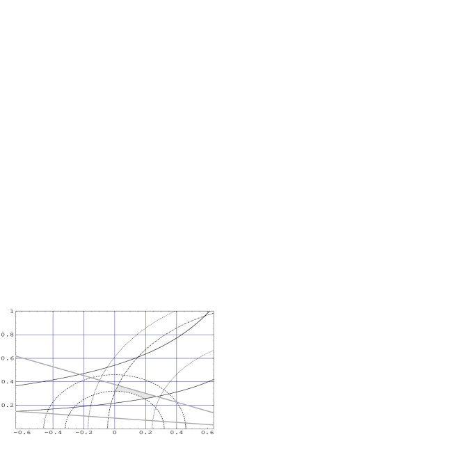
$\bar{\rho}$

FIG. 1.: Determination of the apex $(\bar{\rho},\bar{\eta})$ of the unitarity triangle: The grey region is the presently allowed region, which is determined by (a) the measurement of $|V_{ub}/V_{cb}|$ (corresponding to the dashed circles), (b) the observed $B_{d}^{0}-\bar{B}_{d}^{0}$ mixing parameter $\Delta m_{d}$ (corresponding to the dotted circles), (c) the upper bound on the $B_{s}^{0}-\bar{B}_{s}^{0}$ mixing parameter $\Delta m_{s}$ (which corresponds to the dashed-dotted circle), (d) the measurement of $\epsilon_{K}$ (corresponding to the solid hyperbolae) and (e) the combined result of the CDF, BELLE and BaBar measurements of $a_{\psi K_{S}}$ (thick grey lines).

$a_{\pi\nu\bar{\nu}}$

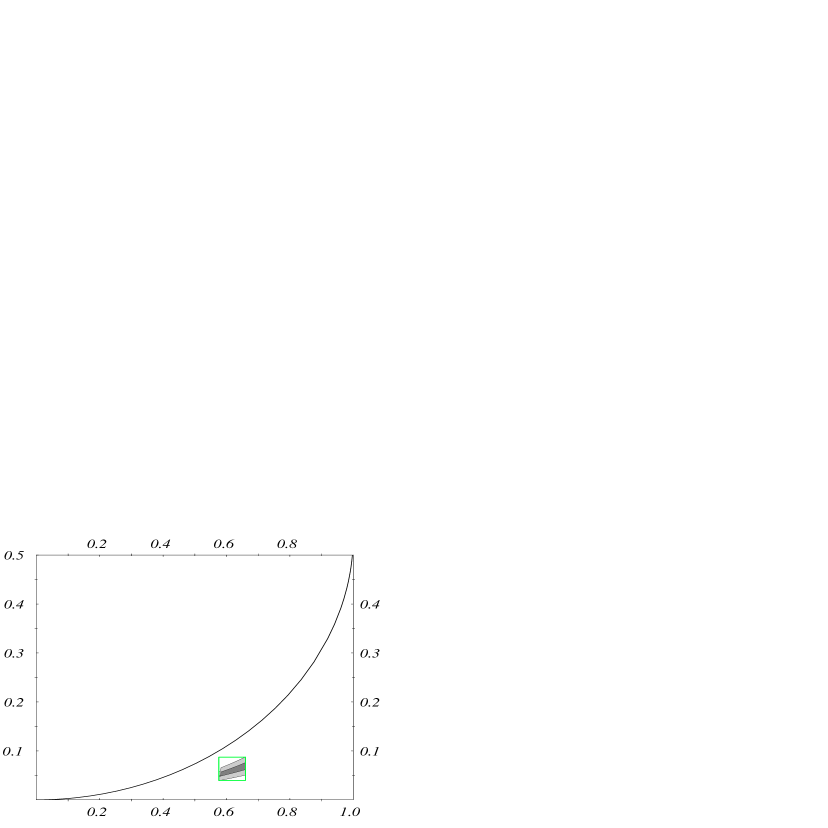
$a_{\psi K_{S}}$

FIG. 2.: Relation between $a_{\pi\nu\bar{\nu}}$ and $a_{\psi K_{S}}$ in the SM: The solid curves displays $a_{\pi\nu\bar{\nu}}(a_{\psi K_{S}})$ for $\Delta=0$. Only in this case there is a one-to-one correspondence between $a_{\pi\nu\bar{\nu}}$ and $a_{\psi K_{S}}$. A scan over the presently allowed region in the $(\bar{\rho},\bar{\eta})$ plane (see Fig. 1) yields the dark area in the $a_{\psi K_{S}}-a_{\pi\nu\bar{\nu}}$ plane, when taking the central value $\Delta=0.425$. The light region corresponds to the interval $\Delta\in[0.31,0.54]$.

$a_{\pi\nu\bar{\nu}}$

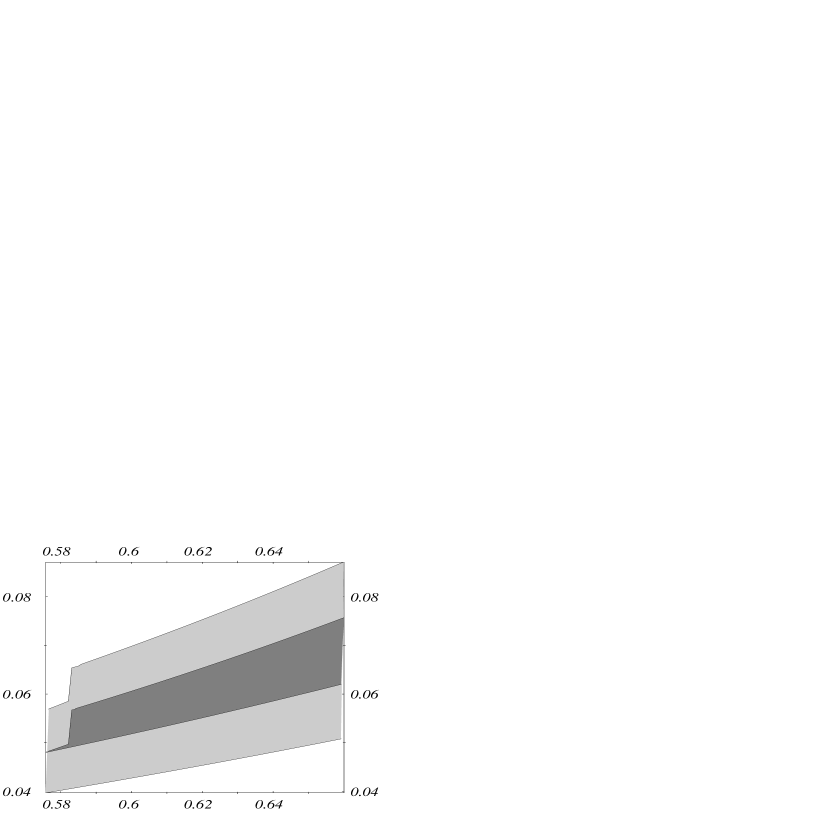
$a_{\psi K_{S}}$

FIG. 3.: Relation between $a_{\pi\nu\bar{\nu}}$ and $a_{\psi K_{S}}$ in the SM. Taking $\Delta=0.425$ yields the dark area in the $a_{\psi K_{S}}-a_{\pi\nu\bar{\nu}}$ plane. The light region corresponds to the interval $\Delta\in[0.31,0.54]$.

$\mbox{BR}(K^{+}\to\pi^{+}\nu\bar{\nu})\times 10^{11}$

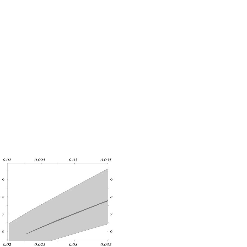
$R_{\Delta m_{B}}$

FIG. 4.: Relation between $\mbox{BR}(K^{+}\to\pi^{+}\nu\bar{\nu})$ and $R_{\Delta m_{B}}$ in the SM: A scan over the presently allowed region for ($\bar{\rho},\bar{\eta}$) (c.f. Fig. 1) yields the dark (light) region in the $R_{\Delta m_{B}}-\mbox{BR}(K^{+}\to\pi^{+}\nu\bar{\nu})$ plane for the central values (total intervals) of the parameters $X^{2}(x_{t}),A,\Delta$ and $\xi$.

$a_{\psi\phi}$

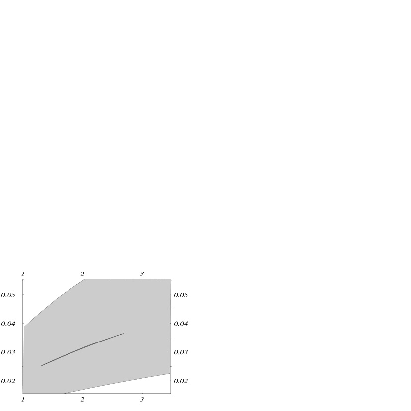
$\mbox{BR}(K_{L}\to\pi^{0}\nu\bar{\nu})\times 10^{11}$

FIG. 5.: Relation between $a_{\psi\phi}$ and $\mbox{BR}(K_{L}\to\pi^{0}\nu\bar{\nu})$ in the SM: A scan over the presently allowed region for ($\bar{\rho},\bar{\eta})$ (c.f. Fig. 1) yields the dark (light) region in the $\mbox{BR}(K_{L}\to\pi^{0}\nu\bar{\nu})-a_{\psi\phi}$ plane for the central values (total intervals) of the parameters $X^{2}(x_{t}),A,\xi$ and ${\cal D}$.

$\mbox{BR}(K_{L}\to\pi^{0}\nu\bar{\nu})\times 10^{11}$

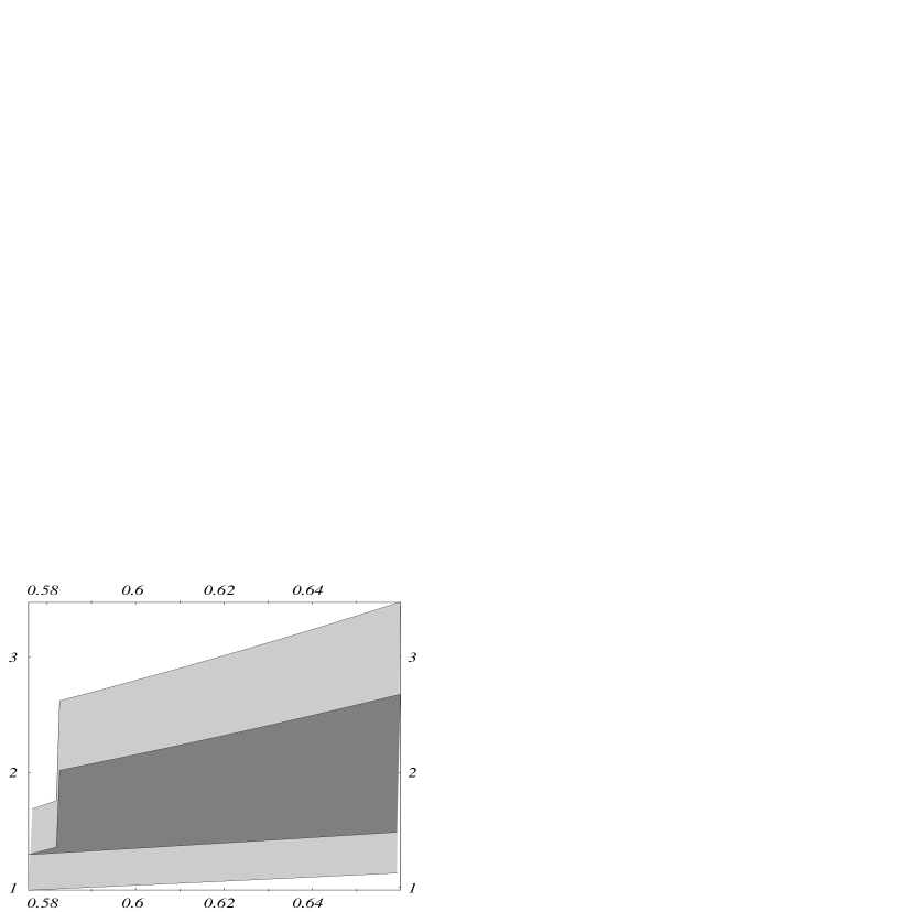
$a_{\psi K_{S}}$

FIG. 6.: Relation between $\mbox{BR}(K_{L}\to\pi^{0}\nu\bar{\nu})$ and $a_{\psi K_{S}}$ in the SM: A scan over the presently allowed region for ($\bar{\rho},\bar{\eta}$) (c.f. Fig. 1) yields the dark (light) region in the $a_{\psi K_{S}}-\mbox{BR}(K_{L}\to\pi^{0}\nu\bar{\nu})$ plane for the central values (total intervals) of the parameters $X^{2}(x_{t})$ and $A$.

$\mbox{BR}(K_{L}\to\pi^{0}\nu\bar{\nu})\times 10^{11}$

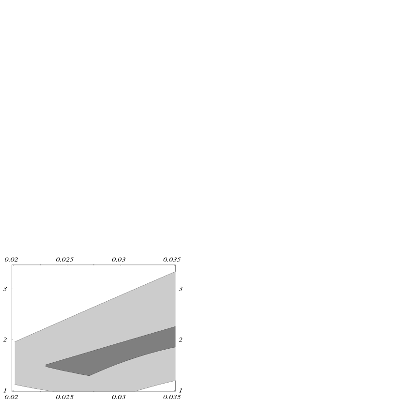
$R_{\Delta m_{B}}$

FIG. 7.: Relation between $\mbox{BR}(K_{L}\to\pi^{0}\nu\bar{\nu})$ and $R_{\Delta m_{B}}$ in the SM: A scan over the presently allowed region for ($\bar{\rho},\bar{\eta}$) (c.f. Fig. 1) yields the dark (light) region in the $R_{\Delta m_{B}}-\mbox{BR}(K_{L}\to\pi^{0}\nu\bar{\nu})$ plane for the central values (total intervals) of the parameters $\xi,X^{2}(x_{t})$ and $A$.