Screened Perturbation Theory to Three Loops

Abstract

The thermal physics of a massless scalar field with a $\phi^{4}$ interaction is studied within screened perturbation theory (SPT). In this method the perturbative expansion is reorganized by adding and subtracting a mass term in the lagrangian. We consider several different mass prescriptions that generalize the one-loop gap equation to two-loop order. We calculate the pressure and entropy to three-loop order and the screening mass to two-loop order. In contrast to the weak-coupling expansion, the SPT-improved approximations appear to converge even for rather large values of the coupling constant.

I Introduction

If we have a weakly-coupled quantum field theory in equilibrium at temperature $T$, we should be able to use perturbation theory as a quantitative tool to study its properties. In the case of a massless theory with coupling constant $g$, the naive perturbative expansion in powers of $g^{2}$ breaks down because of collective effects such as screening. However, the perturbative expansion can be reorganized into a weak-coupling expansion in powers of $g$ either by using resummation methods or alternatively by using effective field theory. It is reasonable to assume that this weak-coupling expansion provides a useful asymptotic expansion for sufficiently small values of $g$.

Only in recent years has the calculational technology of thermal quantum field theory advanced to the point where this assumption can be tested. Unfortunately, the assumption seems to be false. One would expect the thermodynamic functions, such as the pressure, to be among the quantities with the best-behaved weak-coupling expansion, since collective effects are suppressed by several powers of $g$. However, in recent years, the thermodynamic functions have been calculated to order $g^{5}$ for massless scalar theories [1, 2, 3], abelian gauge theories [4, 5], and nonabelian gauge theories [1, 6, 7]. The weak-coupling expansions show no sign of converging even for extremely small values of $g$. There is already a hint of the problem in the $g^{3}$ correction, which has the opposite sign and is relatively large compared to the $g^{2}$ coefficient. The large size of the $g^{3}$ contribution is not necessarily fatal, since it is the first term that takes into account collective effects. An optimist might still hope that higher-order corrections would be well-behaved. This optimism has been dashed by the explicit calculation of the $g^{4}$ and $g^{5}$ terms.

For a massless scalar field theory with a $g^{2}\phi^{4}/4!$ interaction, the weak-coupling expansion for the pressure to order $g^{5}$ is [1, 2, 3]

$${\cal P} = {\cal P}_{\rm ideal}\left[1-{5\over 4}\alpha+{5\sqrt{6}\over 3}\alpha^{3/2}+{15\over 4}\left(\log{\mu\over 2\pi T}+0.40\right)\alpha^{2}\right.$$ (2)

$$\left.-{15\sqrt{6}\over 2}\left(\log{\mu\over 2\pi T}-{2\over 3}\log\alpha-0.72\right)\alpha^{5/2}+{\cal O}(\alpha^{3}\log\alpha)\right]\;,$$

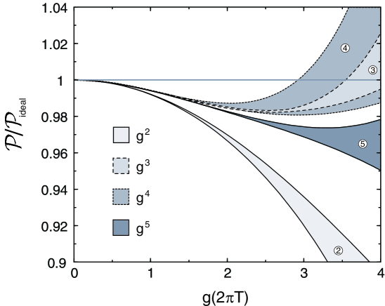
where ${\cal P}_{\rm ideal}=(\pi^{2}/90)T^{4}$ is the pressure of an ideal gas of free massless bosons, $\alpha=g^{2}(\mu)/16\pi^{2}$, and $g(\mu)$ is the $\overline{\rm MS}$ coupling constant at the renormalization scale $\mu$. In Fig. 1, we show the successive perturbative approximations to ${\cal P}/{\cal P}_{\rm ideal}$ as a function of $g(2\pi T)$. Each partial sum is shown as a band obtained by varying $\mu$ from $\pi T$ to $4\pi T$. To express $g(\mu)$ in terms of $g(2\pi T)$, we use the numerical solution to the renormalization group equation $\mu{\partial\over\partial\mu}\alpha=\beta(\alpha)$ with a five-loop beta function [8]:

$$\mu{\partial\over\partial\mu}\alpha=3\alpha^{2}-{17\over 3}\alpha^{3}+32.54\alpha^{4}-271.6\alpha^{5}+2848.6\alpha^{6}\;.$$ (3)

The lack of convergence of the weak-coupling expansion is evident in Fig. 1. The band obtained by varying $\mu$ by a factor of two is not necessarily a good measure of the error, but it is certainly a lower bound on the theoretical error. Another indicator of the theoretical error is the deviation between successive approximations. We can infer from Fig. 1 that the error grows rapidly when $g(2\pi T)$ exceeds 1.5.

FIG. 1.: Weak-coupling expansion to orders $g^{2}$, $g^{3}$, $g^{4}$, and $g^{5}$ for the pressure normalized to that of an ideal gas as a function of $g(2\pi T)$.

A similar behavior can be seen in the weak-coupling expansion for the screening mass, which has been calculated to next-to-next-to-leading order in $g$ [3]:

$$m_{s}^{2}={2\pi^{2}\over 3}\alpha T^{2}\Bigg{\{}1-\sqrt{6}\alpha^{1/2}-\left[3\log{\mu\over 2\pi T}-2\log\alpha-6.4341\right]\alpha+{\cal O}(\alpha^{3/2})\Bigg{\}}\;.$$ (4)

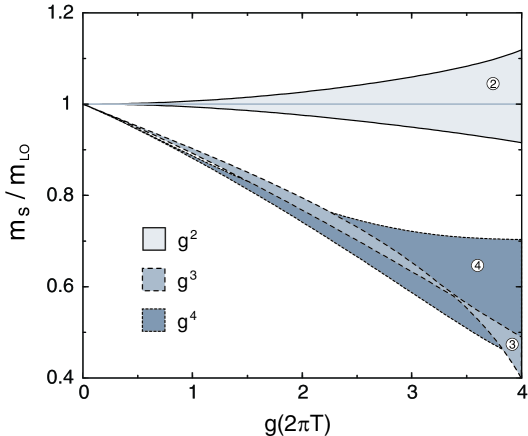
In Fig. 2, we show the screening mass $m_{s}$ normalized to the leading order result $m_{LO}=g(2\pi T)T/\sqrt{24}$ as a function of $g(2\pi T)$, for each of the three successive approximations to $m_{s}^{2}$. The bands correspond to varying $\mu$ from $\pi T$ to $4\pi T$. The poor convergence is again evident. The pattern is similar to that in Fig. 1, with a large deviation between the order-$g^{2}$ and order-$g^{3}$ approximations and a large increase in the size of the band for $g^{4}$.

FIG. 2.: Weak-coupling expansion to orders $g^{2}$, $g^{3}$, and $g^{4}$ for the screening mass normalized to the leading-order expression as a function of $g(2\pi T)$.

There are many possibilities for reorganizing the weak-coupling expansion to improve its convergence. One possibility is to use Padé approximants [9]. This method is limited to observables like the pressure, for which several terms in the weak-coupling expansion are known. Its application is further complicated by the appearance of logarithms of the coupling constant in the coefficients of the weak-coupling expansion. However, the greatest problem with Padé approximants is that, with no understanding of the analytic behavior of ${\cal P}$ at strong coupling, it is little more than a numerological recipe.

An alternative with greater physical motivation is a self-consistent approach [10]. Perturbation theory can be reorganized by expressing the free energy as a stationary point of a functional $\Omega$ of the exact self-energy function $\Pi(p_{0},{\bf p})$ called the thermodynamic potential [11]. Since the exact self-energy is not known, $\Pi$ can be regarded as a variational function. The “$\Phi$-derivable” prescription of Baym [10] is to truncate the perturbative expansion for the thermodynamic potential $\Omega$ and to determine $\Pi$ self-consistently as a stationary point of $\Omega$. This gives an integral equation for $\Pi$ which is difficult to solve numerically, except in cases where $\Pi$ is momentum independent. In relativistic field theories, there are additional complications from ultraviolet divergences. A more tractable approach is to find an approximate solution to the integral equations that is accurate only in the weak-coupling limit. Such an approach has been applied by Blaizot, Iancu, and Rebhan to massless scalar field theories and gauge theories [12, 13].

Another approach that is also variational in spirit is screened perturbation theory (SPT) introduced by Karsch, Patkós and Petreczky [14]. This approach is less ambitious than the $\Phi$-derivable approach. Instead of introducing a variational function, it introduces a single variational parameter $m$. This parameter has a simple and obvious physical interpretation as a thermal mass. The advantage of screened perturbation theory is that it is very easy to apply. Higher order corrections are tractable, so one can test whether it improves the convergence of the weak-coupling expansion. Karsch, Patkós and Petreczky applied screened perturbation theory to a massless scalar field theory with a $\phi^{4}$ interaction, computing the two-loop pressure and the three-loop pressure in the large-$N$ limit. In both cases, they used a one-loop gap equation as their prescription for the mass. Their three-loop calculation was not a very stringent test of the method, because the large-$N$ limit suppresses self-energy diagrams that depend on the momentum.

In this paper, we present a thorough study of screened perturbation theory for a massless scalar field theory with a $\phi^{4}$ interaction. We calculate the pressure and entropy to three loops and the screening mass to two loops using SPT. We consider several generalizations of the one-loop gap equation to two loops. Inserting the solutions to the gap equations for $m$ into the SPT expansions, we obtain the SPT-improved approximations to the pressure, the screening mass, and the entropy.

The paper is organized as follows. In section II, we describe the systematics of screened perturbation theory. In section III, we discuss the possible prescriptions that can be used to generalize the one-loop gap equation to higher orders. We calculate the free energy to three-loop order in section IV and the screening mass to two-loop order in section V. In section VI, we study three generalizations of the one-loop gap equation to two-loop order. In section VII, we study the convergence of the SPT-improved results for the pressure, screening mass, and entropy. In section VIII, we summarize and conclude. We have collected the necessary sum-integrals in an appendix.

II Screened Perturbation Theory

The lagrangian density for a massless scalar field with a $\phi^{4}$ interaction is

$${\cal L}={1\over 2}\partial_{\mu}\phi\partial^{\mu}\phi-{1\over 24}g^{2}\phi^{4}+\Delta{\cal L}\;,$$ (5)

where $g$ is the coupling constant and $\Delta{\cal L}$ includes counterterms. The conventional perturbative expansion in powers of $g^{2}$ generates ultraviolet divergences, and the counterterm $\Delta{\cal L}$ must be adjusted to cancel the divergences order by order in $g^{2}$. If we use dimensional regularization in $d=3-2\epsilon$ spatial dimensions and minimal subtraction to remove the ultraviolet divergences, the counterterms have the form

$$\Delta{\cal L}={1\over 2}\left(Z_{\phi}-1\right)\partial_{\mu}\phi\partial^{\mu}\phi-{1\over 24}\Delta g^{2}\phi^{4},$$ (6)

where $\Delta g^{2}=\left(Z_{\phi}^{2}Z_{g}-1\right)g^{2}$, and $Z_{\phi}$ and $Z_{g}$ are power series in $g^{2}$ whose coefficients have poles in $\epsilon$. At nonzero temperature, the conventional perturbative expansion also generates infrared divergences. They can be removed by resumming the higher order diagrams that generate a thermal mass of order $gT$ for the scalar particle. This resummation changes the perturbative series from an expansion in powers of $g^{2}$ to an expansion in powers of $\left(g^{2}\right)^{1/2}=g$.

Screened perturbation theory, which was introduced by Karsch, Patkós and Petreczky [14], is simply a reorganization of the perturbation series for thermal field theory. It can be made more systematic by using a framework called “optimized perturbation theory” that Chiku and Hatsuda [15] have applied to a spontaneously broken scalar field theory. The lagrangian density is written as

$${\cal L}_{\rm SPT}=-{\cal E}_{0}+{1\over 2}\partial_{\mu}\phi\partial^{\mu}\phi-{1\over 2}(m^{2}-m_{1}^{2})\phi^{2}-{1\over 24}g^{2}\phi^{4}+\Delta{\cal L}+\Delta{\cal L}_{\rm SPT}\;,$$ (7)

where ${\cal E}_{0}$ is a vacuum energy density parameter and we have added and subtracted mass terms. If we set ${\cal E}_{0}=0$ and $m_{1}^{2}=m^{2}$, we recover the original lagrangian (5). Screened perturbation theory is defined by taking $m^{2}$ to be of order $g^{0}$ and $m_{1}^{2}$ to be of order $g^{2}$, expanding systematically in powers of $g^{2}$, and setting $m_{1}^{2}=m^{2}$ at the end of the calculation. This defines a reorganization of perturbation theory in which the expansion is around the free field theory defined by

$${\cal L}_{\rm free}=-{\cal E}_{0}+{1\over 2}\partial_{\mu}\phi\partial^{\mu}\phi-{1\over 2}m^{2}\phi^{2}\;.$$ (8)

The interaction term is

$${\cal L}_{\rm int}={-}{1\over 24}g^{2}\phi^{4}+{1\over 2}m_{1}^{2}\phi^{2}+\Delta{\cal L}+\Delta{\cal L}_{\rm SPT}\;.$$ (9)

At each order in screened perturbation theory, the effects of the $m^{2}$ term in (8) are included to all orders. However, when we set $m_{1}^{2}=m^{2}$, the dependence on $m$ is systematically subtracted out at higher orders in perturbation theory by the $m_{1}^{2}$ term in (9). At nonzero temperature, screened perturbation theory does not generate any infrared divergences, because the mass parameter $m^{2}$ in the free lagrangian (8) provides an infrared cutoff. The resulting perturbative expansion is therefore a power series in $g^{2}$ and $m_{1}^{2}=m^{2}$ whose coefficients depend on the mass parameter $m$.

This reorganization of perturbation theory generates new ultraviolet divergences, but they can be canceled by the additional counterterms in $\Delta{\cal L}_{\rm SPT}$. The renormalizability of the lagrangian in (7) guarantees that the only counterterms required are proportional to 1, $\phi^{2}$, $\partial_{\mu}\phi\partial^{\mu}\phi$, and $\phi^{4}$. With dimensional regularization and minimal subtraction, the coefficients of these operators are polynomials in $\alpha=g^{2}/16\pi^{2}$ and $m^{2}-m_{1}^{2}$. The extra counterterms required to remove the additional ultraviolet divergences are

$$\Delta{\cal L}_{\rm SPT}=-\Delta{\cal E}_{0}-{1\over 2}\left(\Delta m^{2}-\Delta m_{1}^{2}\right)\phi^{2}\;.$$ (10)

The vacuum energy counterterm has the form $\Delta{\cal E}_{0}=Z_{E}\left(m^{2}-m_{1}^{2}\right)^{2}$, where $Z_{E}$ is a power series in $\alpha$ whose coefficients have poles in $\epsilon$. The mass counterterms have the form $\Delta m^{2}=(Z_{\phi}Z_{m}-1)m^{2}$ and $\Delta m^{2}_{1}=(Z_{\phi}Z_{m}-1)m^{2}_{1}$, where $Z_{\phi}$ is the same wavefunction renormalization constant that appears in (6) and $Z_{m}$ is also a power series in $\alpha$ whose coefficients have poles in $\epsilon$.

Several terms in the power series expansions of the counterterms are known from previous calculations at zero temperature. The counterterms $\Delta g^{2}$ and $\Delta m^{2}$ are known to order $\alpha^{5}$ [8]. We will need the coupling constant counterterm only to leading order in $\alpha$:

$$\Delta g^{2}=\left[{3\over 2\epsilon}\alpha+...\right]g^{2}\;.$$ (11)

We need the mass counterterms $\Delta m^{2}$ and $\Delta m^{2}_{1}$ to next-to-leading order and leading order in $\alpha$, respectively:

$$\Delta m^{2} = \left[{1\over 2\epsilon}\alpha+\left({1\over 2\epsilon^{2}}-{5\over 24\epsilon}\right)\alpha^{2}+...\right]m^{2}\;,$$ (12)

$$\Delta m^{2}_{1} = \left[{1\over 2\epsilon}\alpha+...\right]m^{2}_{1}\;.$$ (13)

The counterterm for $\Delta{\cal E}_{0}$ has been calculated to order $\alpha^{4}$ [16]. We will need its expansion only to second order in $\alpha$ and $m_{1}^{2}$:

$$(4\pi)^{2}\Delta{\cal E}_{0} = \left[{1\over 4\epsilon}+{1\over 8\epsilon^{2}}\alpha+\left({5\over 48\epsilon^{3}}-{5\over 72\epsilon^{2}}+{1\over 96\epsilon}\right)\alpha^{2}\right]m^{4}$$ (15)

$$-2\left[{1\over 4\epsilon}+{1\over 8\epsilon^{2}}\alpha\right]m_{1}^{2}m^{2}+{1\over 4\epsilon}m_{1}^{4}\;.$$

III Mass Prescriptions

The mass parameter $m$ in screened perturbation theory is completely arbitrary. To complete a calculation in screened perturbation theory, it is necessary to specify $m$ as a function of $g$ and $T$. One of the complications from the ultraviolet divergences is that the parameters ${\cal E}_{0}$, $m^{2}$, $g^{2}$, and $m_{1}^{2}$ all become running parameters that depend on a renormalization scale $\mu$. In our prescription for recovering the original theory, we must therefore specify the renormalization scale $\mu_{*}$ at which the lagrangian (7) reduces to (5). The prescription can be written

$${\cal E}_{0}(\mu_{*}) =0 \,,$$ (16)

$$m^{2}(\mu_{*}) = m_{1}^{2}(\mu_{*})=m^{2}_{*}(T),$$ (17)

where $m_{*}(T)$ is some prescribed function of the temperature. This is the only point where temperature enters into SPT. We proceed to discuss the possible prescriptions for $m_{*}(T)$.

The prescription of Karsch, Patkós, and Petreczky for $m_{*}(T)$ is the solution to the one-loop gap equation:

$$m_{*}^{2}={1\over 2}\alpha(\mu_{*})\left[J_{1}(m_{*}/T)T^{2}-\left(2\log{\mu_{*}\over m_{*}}+1\right)m_{*}^{2}\right]\;,$$ (18)

where the function $J_{1}(x)$ is defined in (A.8). Their choice for the scale was $\mu_{*}=T$. In the weak-coupling limit, the solution to (18) is $m_{*}=g(\mu_{*})T/\sqrt{24}$.

There are many possibilities for generalizing (18) to higher orders in $g$. One class of possibilities is to identify $m_{*}$ with some physical mass in the system. The simplest choice is the screening mass $m_{s}$ defined by the location of the pole in the static propagator:

$${\bf p}^{2}+m^{2}+\Pi(0,{\bf p})=0\hskip 28.45274pt{\rm at}\;\;\;{\bf p}^{2}=-m_{s}^{2}\;,$$ (19)

where $\Pi(p_{0},{\bf p})$ is the self-energy function. Another choice is the rest mass of the quasiparticle: $m_{q}={\rm Re}\;\omega(0)$, where $\omega(p)$ is the quasiparticle dispersion relation which satisfies $-\omega^{2}+p^{2}+\Pi(i(\omega+i\epsilon),{\bf p})=0$. The quasiparticle mass is more difficult to calculate than the screening mass.

Another mass prescription that generalizes (18) to higher orders is to identify $m_{*}$ with the tadpole mass defined by $m_{t}^{2}=g^{2}\langle\phi^{2}\rangle$. This can also be expressed as a derivative of the free energy:

$$m_{t}^{2}={\!\!\!\!\partial\over\partial m^{2}}{\cal F}(T,g,m,m_{1},\mu)\Bigg{|}_{m_{1}=m}\;,$$ (20)

where the partial derivative is taken before setting $m_{1}=m$. An advantage of the tadpole mass is that $\langle\phi^{2}\rangle$ is easier to calculate at higher orders than the self-energy $\Pi$.

There is another class of prescriptions that is variational in spirit. The results of SPT would be independent of $m$ if they were calculated to all orders. This suggests choosing $m$ to minimize the dependence of some physical quantity on $m$. Taking that physical quantity to be the free energy, the prescription is

$${\!\!\!d\over dm^{2}}{\cal F}(T,g(\mu),m,m_{1}=m,\mu)=0\;.$$ (21)

We will refer to the solution $m_{v}$ to this equation as the variational mass.

One mass prescription that may seem appealing is to choose $m_{*}(T)$ so that the perturbative approximation is thermodynamically consistent [17]. Given a diagrammatic expansion for ${\cal F}$, the entropy density ${\cal S}$ has a diagrammatic expansion given by

$${\cal S}_{\rm diag} = -{\!\!\partial\over\partial T}{\cal F}(T,g,m,m_{1},\mu)\;,$$ (22)

where the partial derivative $\partial/\partial T$ is taken with all the other variables $g$, $m$, $m_{1}$, and $\mu$ held fixed. The entropy density can also be defined by the thermodynamic relation

$${\cal S}_{\rm thermo} = -{\!\!d\over dT}{\cal F}(T,g(\mu),m=m_{*},m_{1}=m_{*},\mu)\;.$$ (23)

The total derivative takes into account the explicit dependence on $T$, the $T$-dependence of $m_{*}(T)$, and also the $T$-dependence of the running coupling constant if we choose a scale $\mu$ that depends on $T$. If the thermodynamic expansions for ${\cal F}$ and ${\cal S}$ were known to all orders, there would be no dependence on $m$ or $\mu$, and (22) and (23) would be equivalent. If the diagrammatic expansion is truncated and if any of the parameters $g$, $m$, $m_{1}$, and $\mu$ is allowed to depend on $T$, then ${\cal S}$ may not satisfy (23). An approximation is called thermodynamically consistent if ${\cal S}$ satisfies (23) exactly. This requires

$${dg\over dT}{\partial{\cal F}\over\partial g}+{d\mu\over dT}{\partial{\cal F}\over\partial\mu}+{dm\over dT}{\partial{\cal F}\over\partial m}+{dm_{1}\over dT}{\partial{\cal F}\over\partial m_{1}}=0\;.$$ (24)

If ${\cal F}$ were known to all orders, it would be independent of $m$ and $m_{1}$ at $m=m_{1}$. Thermodynamic consistency could then be guaranteed by taking the scale $\mu$ to be any function of $T$ and choosing $g(\mu)$ to be the running coupling constant at that scale. If we only have a perturbative approximation to ${\cal F}$, (24) is satisfied only up to higher order corrections. One way to guarantee thermodynamic consistency is to choose $\mu=am$ with $a$ a constant and impose the condition

$${\!\!\!d\over dm^{2}}{\cal F}(T,g(am),m,m_{1}=m,\mu=am)=0\;.$$ (25)

This differs from the variational gap equation (21) only in that we have set $\mu=am$ before differentiating. This equation does not reduce to the one-loop gap equation (18) at leading order, so we will not consider it any further. We will be satisfied by approximations that are thermodynamically consistent only up to higher orders in perturbation theory.

IV Free Energy to Three Loops

In this section, we calculate the pressure and entropy density to three loops in screened perturbation theory. The diagrams for the free energy that are included at this order are those shown in Fig. 3 together with diagrams involving counterterms.

FIG. 3.: Diagrams for the one-loop (0a), two-loop (1a and 1b), and three-loop (2a, 2b, 2c and 2d) free energy.

A One-loop free energy

The free energy at leading order in $g^{2}$ is

$${\cal F}_{0} = {\cal E}_{0}+{\cal F}_{\rm 0a}+\Delta_{0}{\cal E}_{0}\;,$$ (26)

where $\Delta_{0}{\cal E}_{0}$ is the term of order $g^{0}$ in the vacuum energy counterterm (15). The expression for diagram 0a in Fig. 3 is

$${\cal F}_{\rm 0a} = {1\over 2}\hbox{$\sum$}\!\!\!\!\!\!\int_{P}\log\left[P^{2}+m^{2}\right]\;.$$ (27)

The sum-integral in (27) is over the Euclidean momentum $P=(\omega_{n},{\bf p})$ and we define $P^{2}={\bf p}^{2}+\omega_{n}^{2}$. The sum-integral includes a sum over Matsubara frequencies $\omega_{n}=2\pi nT$ and a dimensionally regularized integral over the momentum ${\bf p}$ with a measure that is defined in Appendix A. In dimensional regularization with $3-2\epsilon$ spatial dimensions, the diagrams for ${\cal F}$ have dimensions (energy)^4-2ϵ. To obtain the renormalized free energy density with dimensions (energy)⁴, we multiply the diagrams by $\mu^{2\epsilon}$, where $\mu$ is an arbitrary renormalization scale, before taking the limit $\epsilon\to 0$. The coupling constant in dimensional regularization is $g\mu^{\epsilon}$, where $g$ is the dimensionless renormalized coupling constant. Including the overall factor of $\mu^{2\epsilon}$ and the factor of $\mu^{\epsilon}$ from the coupling constants, there is a factor of $\mu^{2\epsilon}$ for each sum-integral. We choose to absorb this factor into the measure of the sum-integral.

The sum-integral in (27) is expressed as a function of $\epsilon$ in the Appendix. It has a pole at $\epsilon=0$. The result for the diagram is

$${\cal F}_{\rm 0a} = -{1\over 4(4\pi)^{2}}\left({\mu\over m}\right)^{2\epsilon}\Bigg{\{}\left[{1\over\epsilon}+{3\over 2}+{21+\pi^{2}\over 12}\epsilon+{45+3\pi^{2}+4\psi^{\prime\prime}(1)\over 24}\epsilon^{2}\right]m^{4}+2J_{0}T^{4}\Bigg{\}}\;,$$ (28)

where $J_{0}$ is the function of $m/T$ defined in (A.5). We have kept all terms that contribute through order $\epsilon^{2}$, because they enter into higher order diagrams involving counterterms. The pole in $\epsilon$ in (28) is canceled by the zeroth order term $\Delta_{0}{\cal E}_{0}$ in the counterterm (15). The final result for the one-loop free energy is

$$(4\pi)^{2}{\cal F}_{0} = (4\pi)^{2}{\cal E}_{0}-{1\over 8}(2L+3)m^{4}-{1\over 2}J_{0}T^{4}\;,$$ (29)

where $L=\log(\mu^{2}/m^{2})$ and $J_{0}$ can now be replaced by its value at $\epsilon=0$, which is given in (A.8).

B Two-loop free energy

The contribution to the free energy of order $g^{2}$ is

$${\cal F}_{1} = {\cal F}_{\rm 1a}+{\cal F}_{\rm 1b}+\Delta_{1}{\cal E}_{0}+{\partial{\cal F}_{\rm 0a}\over\partial m^{2}}\Delta_{1}m^{2}\;,$$ (30)

where $\Delta_{1}{\cal E}_{0}$ and $\Delta_{1}m^{2}$ are the terms of order $g^{2}$ in the counterterms (12) and (15), respectively. The expressions for the diagrams 1a and 1b in Fig. 3 are

$${\cal F}_{\rm 1a} = {1\over 8}g^{2}\left(\hbox{$\sum$}\!\!\!\!\!\!\int_{P}{1\over P^{2}+m^{2}}\right)^{2}\,,$$ (31)

$${\cal F}_{\rm 1b} = -{1\over 2}m_{1}^{2}\hbox{$\sum$}\!\!\!\!\!\!\int_{P}{1\over P^{2}+m^{2}}\;.$$ (32)

The results for the diagrams can be expressed as

$${\cal F}_{\rm 1a} = {\alpha\over 8(4\pi)^{2}}\left({\mu\over m}\right)^{4\epsilon}\Bigg{\{}\left[{1\over\epsilon^{2}}+{2\over\epsilon}+{18+\pi^{2}\over 6}+{12+\pi^{2}+\psi^{\prime\prime}(1)\over 3}\epsilon\right]m^{4}$$ (34)

$$\hskip 86.49619pt-2\left[{1\over\epsilon}+1+{12+\pi^{2}\over 12}\epsilon\right]J_{1}m^{2}T^{2}+J_{1}^{2}T^{4}\Bigg{\}}\;,$$

$${\cal F}_{\rm 1b} = -{m_{1}^{2}\over 2(4\pi)^{2}}\left({\mu\over m}\right)^{2\epsilon}\Bigg{\{}-\left[{1\over\epsilon}+1+{12+\pi^{2}\over 12}\epsilon\right]m^{2}+J_{1}T^{2}\Bigg{\}}\;,$$ (35)

where $\alpha=g^{2}/16\pi^{2}$. We have kept all terms that contribute through order $\epsilon$, because they are needed for counterterm diagrams in the three-loop free energy. The poles in $\epsilon$ in (34) and (35) are canceled by the counterterms in (30). The final result for the two-loop free energy is

$$(4\pi)^{2}{\cal F}_{1} = {1\over 2}\left[(L+1)m^{2}-J_{1}T^{2}\right]m_{1}^{2}+{1\over 8}\alpha\left[(L+1)m^{2}-J_{1}T^{2}\right]^{2}\;.$$ (36)

C Three-loop free energy

The contribution to the free energy of order $g^{4}$ is

$${\cal F}_{2} = {\cal F}_{\rm 2a}+{\cal F}_{\rm 2b}+{\cal F}_{\rm 2c}+{\cal F}_{\rm 2d}+\Delta_{2}{\cal E}_{0}+{\partial{\cal F}_{\rm 0a}\over\partial m^{2}}\Delta_{2}m^{2}+{1\over 2}{\partial^{2}{\cal F}_{\rm 0a}\over(\partial m^{2})^{2}}\left(\Delta_{1}m^{2}\right)^{2}$$ (38)

$$\hskip 14.22636pt+\left({\,\partial{\cal F}_{\rm 1a}\over\partial m^{2}}+{\,\partial{\cal F}_{\rm 1b}\over\partial m^{2}}\right)\Delta_{1}m^{2}+{{\cal F}_{\rm 1a}\over g^{2}}\Delta_{1}g^{2}+{{\cal F}_{\rm 1b}\over m_{1}^{2}}\Delta_{1}m_{1}^{2}\;,$$

where we have included all the appropriate counterterms. The expressions for the diagrams 2a, 2b, 2c, and 2d in Fig. 3 are

$${\cal F}_{\rm 2a} = -{1\over 16}g^{4}\left(\hbox{$\sum$}\!\!\!\!\!\!\int_{P}{1\over P^{2}+m^{2}}\right)^{2}\hbox{$\sum$}\!\!\!\!\!\!\int_{Q}{1\over(Q^{2}+m^{2})^{2}}\;,$$ (39)

$${\cal F}_{\rm 2b} = -{1\over 48}g^{4}\hbox{$\sum$}\!\!\!\!\!\!\int_{PQR}{1\over(P^{2}+m^{2})(Q^{2}+m^{2})(R^{2}+m^{2})((P+Q+R)^{2}+m^{2})}\;,$$ (40)

$${\cal F}_{\rm 2c} = {1\over 4}g^{2}m_{1}^{2}\hbox{$\sum$}\!\!\!\!\!\!\int_{P}{1\over P^{2}+m^{2}}\hbox{$\sum$}\!\!\!\!\!\!\int_{Q}{1\over(Q^{2}+m^{2})^{2}}\;,$$ (41)

$${\cal F}_{\rm 2d} = -{1\over 4}m_{1}^{4}\hbox{$\sum$}\!\!\!\!\!\!\int_{P}{1\over(P^{2}+m^{2})^{2}}\;.$$ (42)

The results for these diagrams in the limit $\epsilon\rightarrow 0$ are

$${\cal F}_{\rm 2a} = -{\alpha^{2}\over 16(4\pi)^{2}}\left({\mu\over m}\right)^{6\epsilon}\left\{\left[{1\over\epsilon^{3}}+{2\over\epsilon^{2}}+{12+\pi^{2}\over 4\epsilon}+{8+\pi^{2}+\psi^{\prime\prime}(1)\over 2}\right]m^{4}\right.$$ (45)

$$\hskip 98.16191pt+\left[{1\over\epsilon^{2}}+{2\over\epsilon}+{18+\pi^{2}\over 6}\right]J_{2}m^{4}-2\left[{1\over\epsilon^{2}}+{1\over\epsilon}+{6+\pi^{2}\over 6}\right]J_{1}m^{2}T^{2}$$

$$\left.\hskip 98.16191pt-2\left[{1\over\epsilon}+1\right]J_{1}J_{2}m^{2}T^{2}+{1\over\epsilon}J_{1}^{2}T^{4}+J_{1}^{2}J_{2}T^{4}\right\}\;,$$

$${\cal F}_{\rm 2b} = -{\alpha^{2}\over 48(4\pi)^{2}}\left({\mu\over m}\right)^{6\epsilon}\left\{\left[{2\over\epsilon^{3}}+{23\over 3\epsilon^{2}}+{35+\pi^{2}\over 2\epsilon}+C_{0}\right]m^{4}-\left[{6\over\epsilon^{2}}+{17\over\epsilon}-4C_{1}\right]J_{1}m^{2}T^{2}\right.$$ (47)

$$\hskip 98.16191pt\left.+\left[{6\over\epsilon}+12\right]J_{1}^{2}T^{4}+\left[6K_{2}+4K_{3}\right]T^{4}\;\right\},$$

$${\cal F}_{\rm 2c} = {\alpha m_{1}^{2}\over 4(4\pi)^{2}}\left({\mu\over m}\right)^{4\epsilon}\left\{-\left[{1\over\epsilon^{2}}+{1\over\epsilon}+{6+\pi^{2}\over 6}\right]m^{2}-\left({1\over\epsilon}+1\right)J_{2}m^{2}+{1\over\epsilon}J_{1}T^{2}+J_{1}J_{2}T^{2}\right\}\;,$$ (48)

$${\cal F}_{\rm 2d} = -{m_{1}^{4}\over 4(4\pi)^{2}}\left({\mu\over m}\right)^{2\epsilon}\left\{{1\over\epsilon}+J_{2}\right\}\;,$$ (49)

The poles in $\epsilon$ are canceled by the counterterms in (38). The final result for the free energy is

$$(4\pi)^{2}{\cal F}_{2} = -{1\over 4}\left(L+J_{2}\right)m^{4}_{1}-{\alpha\over 4}(L+J_{2})\left[(L+1)m^{2}-J_{1}T^{2}\right]m_{1}^{2}$$ (53)

$$-{1\over 48}\alpha^{2}\left[\left(5L^{3}+17L^{2}+\mbox{$41\over 2$}L-23-\mbox{$23\over 12$}\pi^{2}-\psi^{\prime\prime}(1)+C_{0}+3(L+1)^{2}J_{2}\right)m^{4}\right.$$

$$\left.\hskip 28.45274pt-\left(12L^{2}+28L-12-\pi^{2}-4C_{1}+6(L+1)J_{2}\right)J_{1}m^{2}T^{2}\right.$$

$$\hskip 28.45274pt\left.+\left(3(3L+4)J_{1}^{2}+3J_{1}^{2}J_{2}+6K_{2}+4K_{3}\right)T^{4}\right]\;.$$

D Pressure to three loops

The pressure ${\cal P}$ is given by $-{\cal F}$. The contributions to the free energy of zeroth, first, and second order in $g^{2}$ are given in (29), (36), and (53), respectively. Adding them and setting ${\cal E}_{0}=0$ and $m_{1}^{2}=m^{2}$, we get the approximations to the pressure in screened perturbation theory. The one-loop approximation is obtained by setting ${\cal E}_{0}=0$ in (29):

$$(4\pi)^{2}{\cal P}_{0}={1\over 8}\left[4J_{0}T^{4}+\left(2L+3\right)m^{4}\right]\;.$$ (54)

The two-loop approximation is obtained by adding (36) with $m_{1}^{2}=m^{2}$:

$$(4\pi)^{2}{\cal P}_{0+1}={1\over 8}\left[4J_{0}T^{4}+4J_{1}m^{2}T^{2}-\left(2L+1\right)m^{4}\right]-{1\over 8}\alpha\left[J_{1}T^{2}-(L+1)m^{2}\right]^{2}\;.$$ (55)

The three-loop approximation is obtained by adding (53) with $m_{1}^{2}=m^{2}$:

$$(4\pi)^{2}{\cal P}_{0+1+2} = {1\over 8}\left[4J_{0}T^{4}+4J_{1}m^{2}T^{2}+2J_{2}m^{4}-m^{4}\right]$$ (60)

$$-{1\over 8}\alpha\left[J_{1}T^{2}-(L+1)m^{2}\right]\left[J_{1}T^{2}+2J_{2}m^{2}+(L-1)m^{2}\right]$$

$$+{1\over 48}\alpha^{2}\left[3J_{2}\left(J_{1}T^{2}-(L+1)m^{2}\right)^{2}+\left(3(3L+4)J_{1}^{2}+6K_{2}+4K_{3}\right)T^{4}\right.$$

$$\hskip 56.9055pt-\left(12L^{2}+28L-12-\pi^{2}-4C_{1}\right)J_{1}m^{2}T^{2}$$

$$\hskip 56.9055pt+\left(5L^{3}+17L^{2}+\mbox{${41\over 2}$}L-23-\mbox{${23\over 12}$}\pi^{2}-\psi^{\prime\prime}(1)+C_{0}\right)m^{4}\Big{]}\;,$$

where $L=\log(\mu^{2}/m^{2})$, $C_{0}=39.429$, $C_{1}=-9.8424$, the $J_{n}$’s are the functions of $m/T$ given in (A.8), and $K_{2}$ and $K_{3}$ are functions of $m/T$ given in Ref. [18]. Note that the dependence on $L$ has canceled from the term proportional to $\alpha^{0}$ in (60).

E Entropy to Three Loops

The perturbative expansion for the entropy density ${\cal S}$ is defined in (23). The one-, two-, and three-loop approximations to ${\cal S}$ are obtained by taking the partial derivatives with respect to $T$, with $\alpha$, $m$, and $\mu$ fixed, of the expressions for the pressure in (54), (55), and (60). The partial derivatives of the functions $J_{n}(\beta m$) can be evaluated using the recursion relation (A.6). The partial derivatives of $K_{n}(\beta m)$ can be evaluated numerically.

The one-loop approximation is obtained by differentiating (54):

$${(4\pi)^{2}}T{\cal S}_{0}=2J_{0}T^{4}+J_{1}m^{2}T^{2}\;.$$ (61)

The two-loop approximation is obtained by differentiating (55):

$${(4\pi)^{2}}T{\cal S}_{0+1}=\left[2J_{0}T^{4}+2J_{1}m^{2}T^{2}+J_{2}m^{4}\right]-{1\over 2}\alpha\left[J_{1}T^{2}-(L+1)m^{2}\right]\left[J_{1}T^{2}+J_{2}m^{2}\right]\;.$$ (62)

The three-loop approximation is obtained by differentiating (60):

$$(4\pi)^{2}T{\cal S}_{0+1+2} = {1\over 2}\left[4J_{0}T^{4}+4J_{1}m^{2}T^{2}+2J_{2}m^{4}+J_{3}m^{6}T^{-2}\right]$$ (70)

$$-{1\over 2}\alpha\left[\left(J_{1}T^{2}+J_{2}m^{2}\right)^{2}-\left(J_{1}T^{2}+J_{2}m^{2}\right)m^{2}\right.$$

$$\left.\hskip 56.9055pt+J_{3}\left(J_{1}T^{2}-(L+1)m^{2}\right)m^{4}T^{-2}\right]$$

$$+{1\over 24}\alpha^{2}\left[3J_{3}\left(J_{1}T^{2}-(L+1)m^{2}\right)^{2}m^{2}T^{-2}\right.$$

$$\left.\hskip 56.9055pt+6J_{2}\left(J_{1}T^{2}-(L+1)m^{2}\right)\left(J_{1}T^{2}+J_{2}m^{2}\right)\right.$$

$$\hskip 56.9055pt+\left(6(3L+4)J_{1}^{2}+12K_{2}+8K_{3}\right)T^{4}-\left(3K_{2}^{\prime}+2K_{3}^{\prime}\right)mT^{3}$$

$$\left.\hskip 56.9055pt+6(3L+4)J_{1}J_{2}m^{2}T^{2}\right.$$

$$\hskip 56.9055pt\left.-\left(12L^{2}+28L-12-\pi^{2}-4C_{1}\right)\left(J_{1}T^{2}+J_{2}m^{2}\right)m^{2}\right]\;.$$

The primes on $K_{2}$ and $K_{3}$ denote differentiation with respect to $\beta m$.

V Screening Mass to Two Loops

In this section, we calculate the screening mass to two loops. The diagrams for the self energy that are included at this order are those shown in Fig. 3 together with diagrams involving counterterms. The screening mass $m_{s}$ is the solution to the equation (19). This equation can be solved order-by-order in powers of $\alpha$ and $m_{1}^{2}$. The solution at zeroth order in $g^{2}$ is simply $m_{s}^{2}=m^{2}$.

FIG. 4.: Diagrams for the one-loop (1a and 1b) and two-loop (2a, 2b and 2c) self-energy.

A One-loop self-energy

The self-energy at first order in $g^{2}$ is

$$\Pi_{1}=\Pi_{\rm 1a}-m_{1}^{2}+\Delta_{1}m^{2}\;,$$ (71)

where $\Delta_{1}m^{2}$ is the mass counterterm of order $\alpha$ given in (12). The expression for the diagram 1a in Fig. 4 is

$$\Pi_{\rm 1a} = {1\over 2}g^{2}\hbox{$\sum$}\!\!\!\!\!\!\int_{P}{1\over P^{2}+m^{2}}\;.$$ (72)

The result for the diagram is

$$\Pi_{\rm 1a} = {1\over 2}\alpha\left({\mu\over m}\right)^{2\epsilon}\Bigg{\{}-\left[{1\over\epsilon}+1+{12+\pi^{2}\over 12}\epsilon\right]m^{2}+J_{1}T^{2}\Bigg{\}}\;.$$ (73)

We have kept all terms that contribute to order $\epsilon$, because they are needed for counterterm diagrams in the two-loop self-energy. The pole in $\epsilon$ in (73) is canceled by the counterterm $\Delta_{1}m^{2}$. The final result for the one-loop self-energy is

$$\Pi_{1}={1\over 2}\alpha\left[J_{1}T^{2}-(L+1)m^{2}\right]-m^{2}_{1}\;.$$ (74)

B Two-loop self-energy

The contribution to the self-energy of second order in $g^{2}$ is

$$\Pi_{2}(P)=\Pi_{\rm 2a}+\Pi_{\rm 2b}(P)+\Pi_{\rm 2c}+{\partial\Pi_{\rm 1a}\over\partial m^{2}}\Delta_{1}m^{2}+{\Pi_{\rm 1a}\over g^{2}}\Delta_{1}g^{2}+\Delta_{2}m^{2}-\Delta_{1}m_{1}^{2}\;.$$ (75)

The expressions for the diagrams 2a and 2b in Fig. 4 are

$$\Pi_{\rm 2a} = -{1\over 4}g^{4}\hbox{$\sum$}\!\!\!\!\!\!\int_{Q}{1\over Q^{2}+m^{2}}\hbox{$\sum$}\!\!\!\!\!\!\int_{R}{1\over(R^{2}+m^{2})^{2}}\;,$$ (76)

$$\Pi_{\rm 2b}(P) = -{1\over 6}g^{4}\hbox{$\sum$}\!\!\!\!\!\!\int_{QR}{1\over Q^{2}+m^{2}}{1\over R^{2}+m^{2}}{1\over(P+Q+R)^{2}+m^{2}}\;,$$ (77)

$$\Pi_{\rm 2c} = {1\over 2}g^{2}m_{1}^{2}\hbox{$\sum$}\!\!\!\!\!\!\int_{Q}{1\over(Q^{2}+m^{2})^{2}}\;.$$ (78)

The diagrams $\Pi_{\rm 2a}$ and $\Pi_{\rm 2c}$ are independent of the momentum $P$. The results for these diagrams in the limit $\epsilon\rightarrow 0$ are

$$\Pi_{\rm 2a} = {1\over 4}\alpha^{2}\left({\mu\over m}\right)^{4\epsilon}\left[\left({1\over\epsilon^{2}}+{1\over\epsilon}+{6+\pi^{2}\over 6}\right)m^{2}+\left({1\over\epsilon}+1\right)J_{2}m^{2}-\left({1\over\epsilon}+J_{2}\right)J_{1}T^{2}\right]\;,$$ (79)

$$\Pi_{\rm 2c} = {1\over 2}\alpha m^{2}_{1}\left({\mu\over m}\right)^{2\epsilon}\left[{1\over\epsilon}+J_{2}\right]\;.$$ (80)

The diagram $\Pi_{\rm 2b}$ depends on the external momentum $P$. The equation (19) for the screening mass involves the self-energy at $p_{0}=0$. To calculate the screening mass to second order in $g^{2}$, we need the analytic continuation of $\Pi(0,{\bf p})$ to ${\bf p}^{2}=-m^{2}$. This is calculated in the appendix. The result is

$$\Pi_{\rm 2b}(0,{\bf p})\Bigg{|}_{{\bf p}^{2}=-m^{2}}={1\over 6}\alpha^{2}\left({\mu\over m}\right)^{4\epsilon}\Bigg{\{}\left[{3\over 2\epsilon^{2}}+{17\over 4\epsilon}-C_{1}\right]m^{2}-3\left[{1\over\epsilon}J_{1}+\tilde{K}_{1}+\tilde{K}_{2}\right]T^{2}\Bigg{\}}\;.$$ (81)

The poles in (79)-(81) are canceled by the counterterms in (75). The final result for the two-loop self-energy at $p_{0}=0$ and ${\bf p}^{2}=-m^{2}$ is

$$\Pi_{2}(0,{\bf p})\Bigg{|}_{{\bf p}^{2}=-m^{2}} = {1\over 2}\alpha(L+J_{2})m_{1}^{2}+{1\over 24}\alpha^{2}\Bigg{\{}\left[12L^{2}+28L-12-\pi^{2}-4C_{1}+6\left(L+1\right)J_{2}\right]m^{2}$$ (83)

$$\hskip 118.36356pt-6\left[\left(3L+J_{2}\right)J_{1}+2\tilde{K}_{1}+2\tilde{K}_{2}\right]T^{2}\Bigg{\}}\;.$$

C Screening mass

Since the dependence of the self-energy on the momentum enters only at order $g^{4}$ and since the leading-order solution to the screening mass is $m_{s}=m$, the solution to the equation (19) to order $g^{4}$ is simply

$$m_{s}^{2}=m^{2}+\Pi(0,{\bf p}^{2})\Bigg{|}_{{\bf p}^{2}=-m^{2}}\;.$$ (84)

We proceed to calculate the expression to order $g^{2}$ and to order $g^{4}$.

The solution to order $g^{2}$ is obtained by inserting the one-loop self-energy (74) into (84). Setting $m_{1}^{2}=m^{2}$, the result is

$$m_{s}^{2}={1\over 2}\alpha\left[J_{1}T^{2}-(L+1)m^{2}\right]\;.$$ (85)

If we choose $m=m_{s}=m_{*}$, this is identical to the one-loop gap equation (18).

The solution to order $g^{4}$ is obtained by inserting the sum of (74) and (83) into (84). Setting $m_{1}^{2}=m^{2}$, the result is

$$m_{s}^{2} = {1\over 2}\alpha\left[J_{1}T^{2}+(J_{2}-1)m^{2}\right]-{1\over 24}\alpha^{2}\Bigg{[}6J_{2}\left(J_{1}T^{2}-(L+1)m^{2}\right)$$ (87)

$$+6\left(3LJ_{1}+2\tilde{K}_{1}+2\tilde{K}_{2}\right)T^{2}-\left(12L^{2}+28L-12-\pi^{2}-4C_{1}\right)m^{2}\Bigg{]}\;.$$

Note that the dependence on $L$ has canceled in the order-$\alpha$ terms.

VI Gap Equations

In this section, we solve the gap equations that determine the arbitrary mass parameter in screened perturbation theory. We consider the one-loop gap equation and three generalizations to a two-loop gap equation.

A One-loop Gap Equation

The one-loop gap equation is given in (18). It is convenient to introduce the gap function defined by

$${\rm G}=m^{2}-{1\over 2}\alpha\left[J_{1}T^{2}-(L+1)m^{2}\right]\;.$$ (88)

The one-loop gap equation is then ${\rm G}=0$. For simplicity of notation, we will often suppress the subscripts $*$ on $m$ and $\mu$.

Before solving the one-loop gap equation, we need to choose a value for $\mu$. It is natural to take $\mu$ to be proportional to one of the two energy scales in the equation, $T$ and $m$. We will consider two possibilities, $\mu=a(2\pi T)$ and $\mu=am$, and allow the coefficient $a$ to vary from ${1\over 2}$ to $2$. Given either of these choices for $\mu$, the gap equation can be solved for $m$ as a function of $\alpha(\mu)$. The renormalization group equation (3) can then be used to express $\alpha(\mu)$ as a function of $\alpha(2\pi T)$.

In the weak-coupling limit $g\rightarrow 0$, the solution to the gap equation G = 0 approaches

$$m_{*}^{2}\longrightarrow{2\pi^{2}\over 3}\alpha(\mu)T^{2}\left[1-\sqrt{6}\alpha^{1/2}-\left(\log{\mu\over 4\pi T}+\gamma-3\right)\alpha+O(\alpha^{3/2})\right]\,.$$ (89)

In the strong-coupling limit $g\rightarrow\infty$, the gap equation reduces to

$$2\log{\mu\over m}+1=8\int_{0}^{\infty}dx\;{x^{2}\over\sqrt{1+x^{2}}}{1\over e^{\beta m\sqrt{1+x^{2}}}-1}\;.$$ (90)

This has a solution only if $\mu>e^{-1/2}m$.

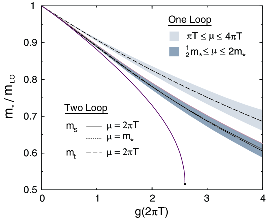
FIG. 5.: Solutions $m_{*}(T)$ to the one-loop gap equation (shaded bands) and the two-loop gap equations (lines) as functions of $g(2\pi T)$.

In Fig. 5, the solutions $m_{*}(T)$ to the one-loop gap equation as a function of $g(2\pi T)$ are shown as bands obtained by varying $\mu$ by a factor of two around the central values $\mu=2\pi T$ and $\mu=m_{*}$, respectively. The solutions are normalized to the leading-order screening mass $m_{LO}=g(2\pi T)T/\sqrt{24}$.

B Screening Gap Equation

The screening gap equation is obtained by identifying $m$ with $m_{s}$. The one-loop expression for the screening mass is given in (85). Thus the one-loop screening gap equation is simply ${\rm G}=0$. The two-loop expression for the screening mass is given in (87). The two-loop screening gap equation can be written as

$$\left[1-{1\over 2}\alpha\left(J_{2}+L\right)\right]{\rm G}+{1\over 24}\alpha^{2}\bigg{[}12\left(LJ_{1}+\tilde{K}_{1}+\tilde{K}_{2}\right)T^{2}$$ (91)

$$-\left(6L^{2}+22L-12-\pi^{2}-4C_{1}\right)m^{2}\bigg{]} = 0\;.$$ (92)

From this expression, it is easy to see that the solution $m$ to the gap equation differs from the solution (89) to the one-loop gap equation by terms of order $\alpha^{2}T^{2}$. The weak-coupling expansion of the solution $m^{2}$ must of course agree through order $\alpha^{2}T^{2}$ with the weak-coupling expansion of $m_{s}^{2}$ given in (4).

The solutions to the screening gap equation for $\mu=2\pi T$ and $\mu=m_{*}$ are shown in Fig. 5. In the case $\mu=2\pi T$, the screening gap equation cannot be continued beyond $g(2\pi T)=2.60$. For $\mu=\pi T$, it terminates at $g(2\pi T)=2.31$, while for $\mu=4\pi T$, it terminates at $g(2\pi T)=3.04$. If we choose $\mu=am_{*}$, the solution can be continued to much larger values of $g$. For $\mu=m_{*}$, it lies very close to the solution to the one-loop gap equation with $\mu=m_{*}$.

C Tadpole Gap Equation

The tadpole mass $m_{t}$ is defined in (20). The one-loop expression is given by differentiating (29). The result is identical to the one-loop expression (85) for the screening mass. To obtain the two-loop expression for the tadpole mass, we add the one- and two-loop free energies (29) and (36), differentiate with respect to $m^{2}$, and then set $m_{1}^{2}=m^{2}$. The result is

$$m_{t}^{2}={1\over 2}\alpha\left[J_{1}T^{2}+(J_{2}-1)m^{2}\right]-{1\over 4}\alpha^{2}\left(J_{2}+L\right)\left[J_{1}T^{2}-(L+1)m^{2}\right]\;.$$ (93)

The order-$\alpha$ term is identical to that of the screening mass (87), but the order-$\alpha^{2}$ term is much simpler.

The one-loop tadpole equation is simply ${\rm G}=0$. The two-loop tadpole gap equation is obtained by setting $m_{t}=m$ in (93). It can be written in the form

$$\left[1-{1\over 2}\alpha\left(J_{2}+L\right)\right]{\rm G}=0\;.$$ (94)

Thus the two-loop tadpole gap equation is identical to the one-loop gap equation: ${\rm G}=0$. The solutions for $\mu=2\pi T$ and $\mu=m_{*}$ are at the centers of the shaded bands in Fig. 5.

D Variational Gap Equation

The variational mass $m_{v}$ is the solution to (21). The one-loop variational gap equation is obtained by differentiating the two-loop expression (55) for the pressure with respect to $m^{2}$ and setting it equal to zero. This gives $\left(L+J_{2}\right)m^{2}{\rm G}=0$, which reduces to the one-loop gap equation: ${\rm G}=0$.

The two-loop variational gap equation is obtained by differentiating the three-loop expression (60) for the pressure. It can be expressed in the form

$$0 = {1\over 4}\alpha(J_{2}+L)^{2}{\rm G}-{1\over 4}\left(J_{3}+{1\over(\beta m)^{2}}\right){\rm G}^{2}/T^{2}$$ (96)

$$\hskip 5.69054pt+{1\over 48}\alpha^{2}\left[-6{J_{1}^{2}\over(\beta m)^{2}}-12(L+2)J_{1}J_{2}+{3K_{2}^{\prime}+2K_{3}^{\prime}\over\beta m}+\;...\;\right]T^{2},$$

where $K_{2}^{\prime}$ and $K_{3}^{\prime}$ are the derivatives of $K_{2}$ and $K_{3}$ with respect to $\beta m$. In the coefficient of $\alpha^{2}T^{2}$, we have written explicitly only the terms that are singular as $\beta m\longrightarrow 0$. The $1/(\beta m)^{2}$ singularities cancel between the $J_{1}^{2}$ and $K_{2}^{\prime}$ term. If we keep the most singular terms in the coefficients of each of the three terms in (96), the equation reduces to

$$0 = {\pi^{2}\alpha\over(\beta m)^{2}}{\rm G}-{\pi\over 4(\beta m)^{3}}{\rm G}^{2}/T^{2}$$ (98)

$$\hskip 5.69054pt-\left[32\pi^{3}(L+2)-(3k_{2}^{\prime}+2k_{3}^{\prime})\log(\beta m)-3(k_{2}+k_{2}^{\prime})-2(k_{3}+k_{3}^{\prime})\right]{\alpha^{2}T^{2}\over 48\beta m}=0\;,$$

where $k_{2}^{\prime}\log(\beta m)+k_{2}$ and $k_{3}^{\prime}\log(\beta m)+k_{3}$ are the coefficients of $\beta m$ in the small-$\beta m$ expansions of $K_{2}$ and $K_{3}$, which are given in (A.17) and (A.18).

The solution to the quadratic equation (98) for ${\rm G}$ is proportional to $\alpha\beta mT^{2}$. The solution $m^{2}$ to the gap equation therefore differs from the solution (89) to the one-loop gap equation by terms of order $\alpha^{3/2}T^{2}$. This is a little disturbing, but even more disturbing is the fact that (98) has no real-valued solutions for G unless $L<2.0984\log(\beta m)+4.1541$. If we assume that $m\to gT/\sqrt{24}$ as $g\to 0$, then this condition is violated for sufficiently small $g$ whether we set $\mu=a(2\pi T)$ or $\mu=am$. Since there are no solutions in the neighborhood of $g=0$, we will not consider the two-loop variational gap equation any further.

VII SPT-improved Observables

In this section, we use the solutions to the gap equation in Sec. VI to obtain successive approximations to the pressure, screening mass, and entropy in screened perturbation theory.

A Pressure

The two-loop SPT-improved approximation to the pressure is obtained by inserting the solution to the one-loop gap equation (18) into the two-loop pressure (55). We can simplify the expression by using (18) to eliminate the explicit appearance of logarithms of $\mu$. Remarkably, this eliminates all the terms of order $\alpha$ and the expression reduces simply to

$$(4\pi)^{2}{\cal P}_{0+1} = {1\over 8}\left[4J_{0}T^{4}+2J_{1}m^{2}T^{2}+m^{4}\right]\;.$$ (99)

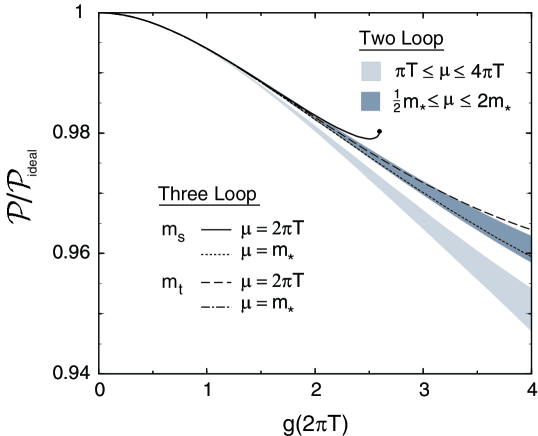
The $J_{0}$ term in (99) is the pressure of an ideal gas of particles of mass $m$. Inserting the solution to the one-loop gap equation shown in Fig. 5, we obtain the bands shown in Fig. 6. The lower and upper bands correspond to varying $\mu$ by a factor of $2$ around the central values $\mu=2\pi T$ and $\mu=m_{*}$, respectively.

FIG. 6.: Two-loop (shaded bands) and three-loop (lines) SPT-improved pressure as a function of $g(2\pi T)$.

The three-loop SPT-improved approximation to the pressure is obtained by inserting the solution to a two-loop gap equation into the three-loop pressure (60). In Fig. 6, we show the three-loop SPT-improved pressure as a function of $g(2\pi T)$ for different two-loop gap equations. The solid line is the result using the two-loop screening gap equation with $\mu=2\pi T$. It cannot be extended past $g(2\pi T)=2.60$. The dashed line is the result using the two-loop tadpole (or one-loop) gap equation with $\mu=2\pi T$. The dotted line is the result using either the two-loop screening gap equation with $\mu_{*}=m_{*}$ or the two-loop tadpole gap equation with $\mu_{*}=m_{*}$. The two are indistinguishable on the scale of the figure. The variations among the three-loop SPT-improved approximations for the pressure are much smaller than one might have expected from the variations among the screening masses. For example, at $g(2\pi T)=2$, the solutions to the two-loop gap equations shown in Fig. 5 vary by about 12%, while the three-loop approximations to the pressure shown in Fig. 6 vary only by about 0.07%.

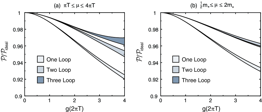
Since the solution to the screening gap equation at $\mu=a(2\pi T)$ cannot be continued beyond a critical value of $g$ and the solution for $\mu=am_{*}$ is close to the solution to the tadpole gap equation for $\mu=am_{*}$, we will consider only the tadpole gap equation from now on. In Fig. 7, we show the one-, two-, and three-loop SPT-improved approximations to the pressure using the tadpole gap equation. The bands are obtained by varying $\mu$ by a factor of two around the central values $\mu=2\pi T$ and $\mu=m_{*}$. The one-loop bands in Fig. 7 lie below the other bands; however, the two- and three-loop bands all lie within the $g^{5}$ band of the weak-coupling expansion in Fig. 1. The one-, two-, and three-loop approximations to the pressure are perturbatively correct up to order $g^{1}$, $g^{3}$, and $g^{5}$, respectively; however, we see a dramatic improvement in the apparent convergence compared to the weak-coupling expansion.

The choice $\mu=am_{*}$ appears to give better convergence than $\mu=a(2\pi T)$, with the three-loop band falling within the two-loop band. The bands for $\mu=am_{*}$ are narrower than those for $\mu=a(2\pi T)$ partly because $\mu=a(2\pi T)$ is larger and therefore closer to the Landau pole of the running coupling constant. If $g(2\pi T)=2$, the Landau pole associated with the five-loop beta function is far away at $\mu=2.11\times 10^{5}(2\pi T)$. If $g(2\pi T)=4$, the Landau pole is rather nearby at $\mu=5.49(2\pi T)$. The coupling constant $g(m_{*})$ is smaller than $g(2\pi T)$, having the values 1.76 and 3.07 if $g(2\pi T)=2$ and $4$, respectively. Choosing $\mu=am_{*}$ instead of $\mu=a(2\pi T)$ will therefore make the error due to the $m^{4}$ terms in the pressure smaller by factors of about 0.60 and 0.35 respectively. The band $m_{*}/2<\mu<2m_{*}$ may therefore give an underestimate of the error of SPT.

FIG. 7.: One-, two-, and three-loop SPT-improved pressure as a function of $g(2\pi T)$ for (a) $\pi T<\mu<4\pi T$ and (b) ${1\over 2}m_{*}<\mu<2m_{*}$.

B Screening Mass

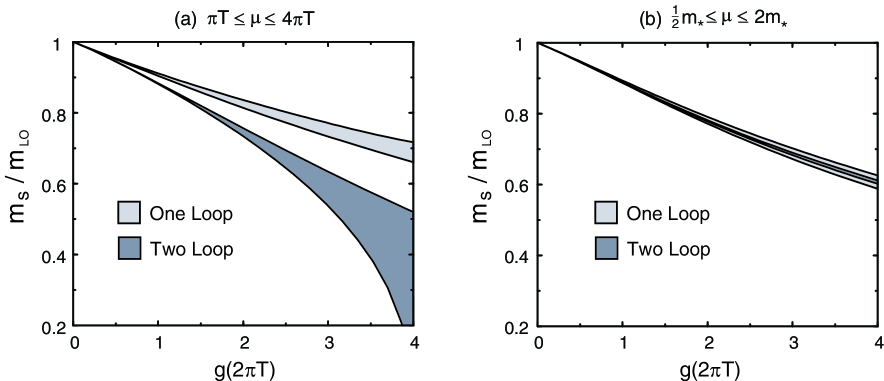
The one-loop SPT-improved approximation to the screening mass $m_{s}$ is simply the solution $m_{*}(T)$ to the tadpole gap equation. A two-loop SPT-improved approximation can be obtained by inserting the solution to the gap equation for $m$ into (87). In Fig. 8, we show the one-loop and two-loop SPT-improved approximations to the screening mass as functions of $g(2\pi T)$. The bands are obtained by varying $\mu$ by a factor of two around the central values $\mu=2\pi T$ and $\mu=m_{*}$.

The choice $\mu=am_{*}$ appears again to give better convergence than $\mu=a(2\pi T)$, with the two-loop band falling within the one-loop band. With $\mu=am_{*}$, there is a dramatic improvement in apparent convergence over the weak-coupling approximations, which are plotted on the same scale in Fig. 2. However, there is not much improvement in the apparent convergence with $\mu=a(2\pi T)$. The conservative conclusion is that screened perturbation theory is not as effective in improving the prediction for the screening mass as it is for the pressure.

FIG. 8.: One-loop and two-loop SPT-improved screening mass as a function of $g(2\pi T)$ for (a) $\pi T<\mu<4\pi T$ and (b) ${1\over 2}m_{*}<\mu<2m_{*}$.

C Entropy

The one-, two- and three-loop SPT-improved entropies are obtained by replacing $m$ in the expressions (61)-(70) for ${\cal S}_{0}$, ${\cal S}_{0+1}$, and ${\cal S}_{0+1+2}$ with the solution $m_{*}$ to the one-loop gap equation ${\rm G}=0$. Using the gap equation to eliminate the logarithm $L$, the expression for the two-loop entropy reduces to

$${(4\pi)^{2}}T{\cal S}_{0+1}=2J_{0}T^{4}+J_{1}m^{2}T^{2}\;.$$ (100)

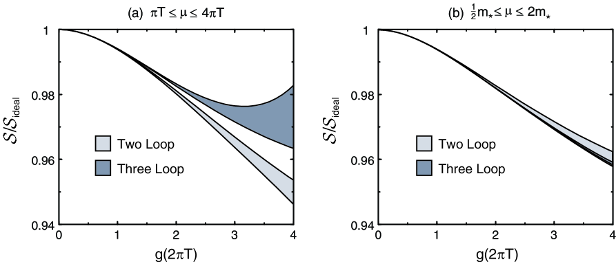
This is identical to the one-loop expression (61), which is the entropy of an ideal gas of particles with mass $m$. In Fig. 9, we show the two- and three-loop SPT-improved approximations to the entropy as functions of $g(2\pi T)$. The entropy density is normalized to that of an ideal gas: ${\cal S}_{\rm ideal}=(2\pi^{2}/45)T^{3}$. The bands in Fig. 9 correspond to varying $\mu$ by a factor of two around the central values $2\pi T$ and $m_{*}$. Once again, the choice $\mu=am_{*}$ seems to give better convergence with the three-loop band lying very close to the two-loop band.

FIG. 9.: Two-loop and three-loop SPT-improved entropy as a function of $g(2\pi T)$ for (a) $\pi T<\mu<4\pi T$, (b) ${1\over 2}m_{*}<\mu<2m_{*}$.

The entropies shown in Fig. 9 are successive approximations to the diagrammatic entropy defined by Eq. 22. However, the entropy can also be defined by the thermodynamic relation (23). Thus successive approximations to ${\cal S}$ can be obtained by differentiating the pressures shown in Fig. 7 with respect to $T$. In that figure we show the ratio of the pressure to that of an ideal gas as a function of $g(2\pi T)$. Defining the function $f(g)$ by

$${\cal P}(T)={\cal P}_{\rm ideal}(T)f(g(2\pi T))\;,$$ (101)

the thermodynamic entropy is then given by

$${\cal S}_{\rm thermo}(T)\;=\;{\cal S}_{\rm ideal}(T)\left[f(g)+{2\pi^{2}\over g}f^{\prime}(g)\beta(\alpha)\right]\;,$$ (102)

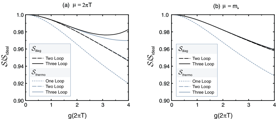
where $g=g(2\pi T)$, $\alpha=g^{2}/16\pi^{2}$, and $\beta(\alpha)$ is the beta function given by the right side of (3). In Fig. 10, the black curves are the two- and three-loop diagrammatic entropies for $\mu=2\pi T$ and $\mu=m_{*}$. The gray curves are the the thermodynamic entropies obtained from the one-, two-, and three-loop SPT-improved pressures. One can see clearly the approach to thermodynamic consistency as one goes from the two-loop to the three-loop approximation. With the choice $\mu=2\pi T$, the two-loop entropy is almost perfectly thermodynamically consistent. However, this is probably an accident because the deviations from thermodynamic entropy are evident in the three-loop entropy. With $\mu=am_{*}$, deviations from thermodynamic consistency are very small for both the two- and three-loop entropies. This is another indication that SPT improvement is more effective if we take the scale $\mu$ to be much lower than $2\pi T$.

FIG. 10.: SPT-improved entropy as a function of $g(2\pi T)$ compared to the thermodynamic entropy for obtained from the SPT-improved pressure for (a) $\mu=2\pi T$ and (b) $\mu=m_{*}$.

VIII Conclusions/Discussion

We have studied the effectiveness of screened perturbation theory in reorganizing the perturbation series for a thermal scalar field theory. We applied it to the pressure and the entropy calculated to three loops and to the screening mass calculated to two loops.

We considered three alternatives for generalizing the one-loop gap equation to two-loop order. The most useful turned out to be the tadpole gap equation, which at two loops is identical to the one-loop gap equation proposed by Karsch, Patkós and Petreczky. The solution to the two-loop variational gap equation does not match onto the one-loop gap equation in the weak-coupling limit. The solution to the two-loop screening gap equation cannot be extended above $g(2\pi T)=2.60$ if we choose the scale to be $\mu=2\pi T$.

The predictions of SPT depend on an arbitrary scale $\mu$ that arises both from the renormalization of the coupling constant and from the renormalization of ultraviolet divergences introduced by screened perturbation theory. These two effects could be separated by introducing two renormalization scales, $\mu_{3}$ and $\mu_{4}$. These scales would be associated with contributions from soft and hard modes respectively as in Ref. [19]. One way disentangle the dependence on these scales would be to evaluate the integrals as expansions in $m/T$. We evaluated our integrals by integrating numerically over all momenta, which precluded any separation of the scales. Instead, we considered two possibilities for the scale, $\mu=m_{*}$ and $\mu=2\pi T$, which correspond to the central values expected for $\mu_{3}$ and $\mu_{4}$, respectively. We allowed for variations of $\mu$ around these central values by factors of two to provide a lower bound on the theoretical uncertainty. The choice $\mu=m_{*}$ gives smaller bands from varying the scale, but this is largely due to the fact that the coupling constant $g(m_{*})$ is smaller than $g(2\pi T)$. Thus the size of the bands is not a good indicator of the success of the SPT improvement.

A better indication of the success of SPT improvement is the stability of the predictions as you go to higher order in the loop expansion. The choice $\mu=2\pi T$ gives a significant improvement in stability for the pressure compared to the weak-coupling expansion. However the SPT improvement seems to be much more effective using $\mu=m_{*}$ than $\mu=2\pi T$. The three-loop band lies within the two-loop band for the pressure and it lies very close for the entropy. The two-loop band also lies within the one-loop band for the screening mass. The two-loop and three-loop approximations for the entropy are also very close to thermodynamic consistency if we choose $\mu=m_{*}$. If we set $\mu=2\pi T$, then going from the two-loop to the three-loop approximations to the pressure or entropy moves the prediction closer to that for $\mu=m_{*}$. This suggests that the SPT-improved prediction for $\mu=m_{*}$ is more accurate than that for $\mu=2\pi T$. All this evidence indicates that SPT improvement is most successful if $\mu$ is taken to be much smaller than $2\pi T$.

To remove the additional ultraviolet divergences introduced by SPT, we have chosen to use dimensional regularization with modified minimal subtraction. This choice is of course not unique. For example, we could have also chosen to subtract the piece of the free energy that is independent of $T$ for fixed $m$, i.e. ${\cal F}_{\rm R}={\cal F}(T,g,m,\mu)-{\cal F}(T=0,g,m,\mu)$. This would result in a different reorganization of the perturbation series that would also agree with the exact result if summed to all orders. We take into account the theoretical uncertainty associated with the choice of subtraction scheme by allowing variation of the renormalization scale $\mu$. For example, by examining Eqs. (54) and (55), we can see that the alternative described above corresponds to $L=-3/2$ or the one-loop approximation and to some value in the range $-{1\over 2}<L<-1$ for the two-loop approximation. Setting $\mu=am_{*}$ with ${1\over 2}<a<2$ corresponds to varying $L$ in the range $-1.4<L<1.4$. Therefore, this variation of $\mu$ does take into account the ambiguity associated with the subtraction scheme at $T=0$ It would of course be preferable to separate the ambiguity from the SPT subtractions from the ambiguity from renormalization of the original theory by allowing separate renormalization scales $\mu_{3}$ and $\mu_{4}$ as mentioned above.

Our results demonstrate the effectiveness of screened perturbation theory in providing stable and apparently converging predictions for the thermodynamic functions of a massless scalar field theory. An essential ingredient of this approach is using the solution to a gap equation as the prescription for the mass parameter $m$. This success of screened perturbation theory adds support to the proposal of Ref. [19] to use HTL perturbation theory to reorganize the weak-coupling expansions for the thermodynamic functions of QCD. In Ref. [19], the free energy was computed only to one-loop order, so there was little alternative to using a weak-coupling expression for the thermal gluon mass parameter. However, our experience with SPT indicates that the stability of the predictions is greatly improved by using a solution to a gap equation for the mass parameter. A gap equation can be derived from the free energy calculated to two-loop order in HTL perturbation theory. Until that calculation is carried out, quantitative comparisons of the predictions of HTL perturbation theory with the nonperturbative results of lattice gauge theory are probably premature.

A Sum-integrals

In the imaginary-time formalism for thermal field theory, a boson has Euclidean four-momentum $P=(p_{0},{\rm\bf p})$, with $P^{2}=p_{0}^{2}+{\rm\bf p}^{2}$. The Euclidean energy $p_{0}$ has discrete values: $p_{0}=2\pi nT$, where $n$ is an integer. Loop diagrams involve sums over $p_{0}$ and integrals over p. We use dimensional regularization to regularize ultraviolet or infrared divergences. Our choice for the measure in the sum-integrals is

$$\hbox{$\sum$}\!\!\!\!\!\!\int_{P}\;\equiv\;\left(\frac{e^{\gamma}\mu^{2}}{4\pi}\right)^{\epsilon}\;T\sum_{p_{0}}\>\int{d^{3-2\epsilon}p\over(2\pi)^{3-2\epsilon}}\,,$$ (A.1)

where $3-2\epsilon$ is the dimension of space and $\mu$ is an arbitrary momentum scale. The factor $(e^{\gamma}/4\pi)^{\epsilon}$ is introduced so that, after minimal subtraction of the poles in $\epsilon$ due to ultraviolet divergences, $\mu$ coincides with the renormalization scale of the $\overline{\rm MS}$ renormalization scheme.

1 One-loop sum-integrals

The one-loop sum-integrals that appear in the free energy can be separated into a temperature-independent term and a term that depends explicitly on $T$:

$$\hbox{$\sum$}\!\!\!\!\!\!\int_{P}\log\left(P^{2}+m^{2}\right) = {1\over(4\pi)^{2}}\left({\mu\over m}\right)^{2\epsilon}\left[-{e^{\gamma\epsilon}\Gamma(1+\epsilon)\over\epsilon(1-\epsilon)(2-\epsilon)}m^{4}-J_{0}T^{4}\right]\;,$$ (A.2)

$$\hbox{$\sum$}\!\!\!\!\!\!\int_{P}\frac{1}{P^{2}+m^{2}} = {1\over(4\pi)^{2}}\left({\mu\over m}\right)^{2\epsilon}\left[-{e^{\gamma\epsilon}\Gamma(1+\epsilon)\over\epsilon(1-\epsilon)}m^{2}+J_{1}T^{2}\right]\;,$$ (A.3)

$$\hbox{$\sum$}\!\!\!\!\!\!\int_{P}\frac{1}{(P^{2}+m^{2})^{2}} = {1\over(4\pi)^{2}}\left({\mu\over m}\right)^{2\epsilon}\left[{e^{\gamma\epsilon}\Gamma(1+\epsilon)\over\epsilon}+J_{2}\right]\;.$$ (A.4)

The thermal terms can be expressed as integrals involving the Bose-Einstein distribution function:

$$J_{n}(\beta m) = {4e^{\gamma\epsilon}\Gamma({1\over 2})\over\Gamma({5\over 2}-n-\epsilon)}\beta^{4-2n}m^{2\epsilon}\int_{0}^{\infty}dk\;{k^{4-2n-2\epsilon}\over\left(k^{2}+m^{2}\right)^{1/2}}{1\over e^{\beta\left(k^{2}+m^{2}\right)^{1/2}}-1}\;.$$ (A.5)

These integrals satisfy the recursion relation

$$xJ_{n}^{\prime}(x)=2\epsilon J_{n}(x)-2x^{2}J_{n+1}(x)\;.$$ (A.6)

The temperature-independent terms in (A.2)–(A.4) can be expanded as a Laurent series around $\epsilon=0$ by using

$$e^{\gamma\epsilon}\Gamma(1+\epsilon)=1+{\pi^{2}\over 12}\epsilon^{2}+{1\over 6}\psi^{\prime\prime}(1)\epsilon^{3}+{\cal O}(\epsilon^{4})\;.$$ (A.7)

The functions $J_{n}$ have Taylor expansions around $\epsilon=0$. They often appear multiplied by poles in $\epsilon$, but it is counterproductive to expand $J_{n}$ in powers of $\epsilon$, because the poles always cancel in physical quantities.

If we set $\epsilon=0$, the integrals $J_{n}$ for $n=0,1,2$ reduce to

$$J_{n}(\beta m)={4\Gamma({1\over 2})\over\Gamma({5\over 2}-n)}\beta^{4-2n}\int_{0}^{\infty}dk\;{k^{4-2n}\over(k^{2}+m^{2})^{1/2}}{1\over e^{\beta(k^{2}+m^{2})^{1/2}}-1}\;.$$ (A.8)

The integral $J_{3}$ requires a subtraction to remove a linear infrared divergence:

$$J_{3}(\beta m)=-2\beta^{-2}\int_{0}^{\infty}dk\;{1\over k^{2}}\left({1\over\left(k^{2}+m^{2}\right)^{1/2}}{1\over e^{\beta(k^{2}+m^{2})^{1/2}}-1}-{1\over m}{1\over e^{\beta m}-1}\right)\;.$$ (A.9)

In the limit $\beta m\longrightarrow 0$, these integrals reduce to

$$J_{0} \longrightarrow {16\pi^{4}\over 45}\;,$$ (A.10)

$$J_{1} \longrightarrow {4\pi^{2}\over 3}\;-\;4\pi\beta m\;-\;2\left(\log{\beta m\over 4\pi}-{1\over 2}+\gamma\right)(\beta m)^{2}\;,$$ (A.11)

$$J_{2} \longrightarrow {2\pi\over\beta m}\;+\;2\left(\log{\beta m\over 4\pi}+\gamma\right)\;,$$ (A.12)

$$J_{3} \longrightarrow {\pi\over(\beta m)^{3}}\;-\;{1\over(\beta m)^{2}}\;+\;{1\over 4\pi^{2}}\zeta(3)\;.$$ (A.13)

2 Basketball sum-integral

The only nontrivial sum-integral required to calculate the free energy to three loops is the massive basketball sum-integral:

$${\cal I}_{\rm ball}=\hbox{$\sum$}\!\!\!\!\!\!\int_{PQR}{1\over(P^{2}+m^{2})(Q^{2}+m^{2})(R^{2}+m^{2})[(P+Q+R)^{2}+m^{2}]}\;.$$ (A.14)

This sum-integral was evaluated in Ref. [20] and the result is

$${\cal I}_{\rm ball} = {1\over(4\pi)^{6}}\left({\mu\over m}\right)^{6\epsilon}\Bigg{\{}\left[{2\over\epsilon^{3}}+{23\over 3\epsilon^{2}}+{35+\pi^{2}\over 2\epsilon}+C_{0}\right]m^{4}+\left[-{6\over\epsilon^{2}}-{17\over\epsilon}+4C_{1}\right]J_{1}m^{2}T^{2}$$ (A.16)

$$\hskip 80.52135pt+\left({6\over\epsilon}+12\right)J_{1}^{2}T^{4}+\left(6K_{2}+4K_{3}\right)T^{4}\Bigg{\}}T^{4}\;,$$

where $C_{0}=39.429$, $C_{1}=-9.8424$, and $K_{2}$ and $K_{3}$ are functions of $\beta m$. They are expressed in Ref. [18] as three-dimensional integrals that can be evaluated numerically. Their behavior in the limit $\beta m\to 0$ is

$$K_{2} \longrightarrow {32\pi^{4}\over 9}\left[\log(\beta m)-0.04597\right]\;-\;372.65\left[\log(\beta m)+1.4658\right]\beta m\;,$$ (A.17)

$$K_{3} \longrightarrow 453.51\;+\;1600.0\left[\log(\beta m)+1.3045\right]\beta m\;.$$ (A.18)

The leading terms are given analytically in Ref. [18]. The terms proportional to $\beta m$ were determined numerically.

3 Sunset sum-integral

The only nontrivial sum-integral required to calculate the self-energy to two loops is the sunset sum-integral, which depends on the external four-momentum $P=(p_{0},{\bf p})$:

$${\cal I}_{\rm sun}(P)=\hbox{$\sum$}\!\!\!\!\!\!\int_{QR}{1\over Q^{2}+m^{2}}{1\over R^{2}+m^{2}}{1\over(P+Q+R)^{2}+m^{2}}\;.$$ (A.19)

This sum-integral can be separated into terms with zero, one, and two thermal distributions, respectively [21]. At $p_{0}=0$, it can be written as

$${\cal I}_{\rm sun}(0,{\bf p})={\cal I}_{\rm sun}^{(0)}({\bf p}^{2})+3{\cal I}_{\rm sun}^{(1)}({\bf p}^{2})+3{\cal I}_{\rm sun}^{(2)}({\bf p}^{2})\;,$$ (A.20)

where

$${\cal I}_{\rm sun}^{(0)}({\bf p}^{2}) = \int_{QR}{1\over Q^{2}+m^{2}}{1\over R^{2}+m^{2}}{1\over(P+Q+R)^{2}+m^{2}}\Bigg{|}_{P=(0,{\bf p)}}\;,$$ (A.21)

$${\cal I}_{\rm sun}^{(1)}({\bf p}^{2}) = \mbox{Re}\int_{q}n\delta(q)\int_{R}{1\over R^{2}+m^{2}}{1\over(P+Q+R)^{2}+m^{2}}\Bigg{|}_{(P+Q)^{2}=-[E_{q}^{2}-({\bf p}+{\bf q})^{2}+i\epsilon]}\;,$$ (A.22)

$${\cal I}_{\rm sun}^{(2)}({\bf p}^{2}) = {\rm Re}\int_{q}n\delta(q)\int_{r}n\delta(r){(-1)\over(p+q+r)^{2}-m^{2}+i\epsilon}\Bigg{|}_{p=(0,{\bf p)}}\;.$$ (A.23)

The integral $\int_{q}$ denotes the dimensionally regularized integral over the Minkowski momentum $(q_{0},{\bf q})$, and $n\delta(q)=n(q_{0})2\pi\delta(q^{2}-m^{2})$.

a Zero thermal factors

To calculate the screening mass to two loops, we need the analytic continuation of the integrals (A.21)-(A.23) to the point ${\bf p}^{2}=-m^{2}$. The integral (A.21) was evaluated in Ref. [18]:

$${\cal I}_{\rm sun}^{(0)}(-m^{2}) = {1\over(4\pi)^{4}}\left({\mu\over m}\right)^{4\epsilon}\left[-{3\over 2\epsilon^{2}}-{17\over 4\epsilon}+C_{1}\right]m^{2}\;,$$ (A.24)

where $C_{1}=-9.8424$.

b One thermal factor

The integral (A.22) can expressed as

$${\cal I}_{\rm sun}^{(1)}({\bf p}^{2}) = {1\over(4\pi)^{4}}\left({\mu\over m}\right)^{4\epsilon}\left[{1\over\epsilon}J_{1}T^{2}\right.$$ (A.26)

$$\left.-8\int_{0}^{\infty}dq\;{q^{2}n(E_{q})\over E_{q}}\int_{0}^{1}dx\left\langle\log{\left|m^{2}-x(1-x)(E_{q}^{2}-k^{2})\right|\over m^{2}}\right\rangle\right]\;,$$

where $k=|{\bf p}+{\bf q}|$ and $\langle...\rangle$ denotes the angular average. After averaging over angles, (A.26) can be analytically continued to ${\bf p}^{2}=-m^{2}$. The result is

$${\cal I}_{\rm sun}^{(1)}(-m^{2}) = {1\over(4\pi)^{4}}\left({\mu\over m}\right)^{4\epsilon}\left[{1\over\epsilon}J_{1}T^{2}+\tilde{K}_{1}T^{2}\right]\;,$$ (A.27)

where $\tilde{K}_{1}$, which is a function of $\beta m$ only, is defined by

$$\tilde{K}_{1}=-{8\over T^{2}}\int_{0}^{\infty}dq\;{q^{2}n(E_{q})\over E_{q}}\int_{0}^{1}dx\;\tilde{f}_{1}(x,q)\;.$$ (A.28)

The function $\tilde{f}_{1}(x,q)$ in the integrand is

$$\tilde{f}_{1}(x,q) = {x^{2}+(1-x)^{2}\over 2x(1-x)q/m}\,\mbox{atan}\,\left({2x(1-x)q/m\over x^{2}+(1-x)^{2}}\right)-1$$ (A.30)

$$+{1\over 2}\log\left(\left[x^{2}+(1-x)^{2}\right]^{2}+4x^{2}(1-x)^{2}q^{2}/m^{2}\right)\;.$$

c Two thermal factors

The integral (A.23) can be expressed as

$${\cal I}_{\rm sun}^{(2)}({\bf p}^{2})={32\over(4\pi)^{4}}\int_{0}^{\infty}dq\;{q^{2}n(E_{q})\over E_{q}}\int_{0}^{\infty}dr\;{r^{2}n(E_{r})\over E_{r}}\sum_{\sigma}\mbox{Re}\left\langle{(-1)\over E_{\sigma}^{2}-k^{2}-m^{2}+i\epsilon}\right\rangle\;,$$ (A.31)

where $E_{\sigma}=E_{q}+\sigma E_{r}$, $k=|{\bf p}+{\bf q}+{\bf r}|$, and $\sigma$ is summed over $\pm 1$. After performing the angular average, (A.31) can be analytically continued to ${\bf p}^{2}=-m^{2}$. The result is

$${\cal I}_{\rm sun}^{(2)}(-m^{2})={1\over(4\pi)^{4}}\tilde{K}_{2}T^{2}\;,$$ (A.32)

where $\tilde{K}_{2}$, which is a function of $\beta m$ only, is defined by

$$\tilde{K}_{2} = {4\over T^{2}}\int_{0}^{\infty}dq\;{qn(E_{q})\over E_{q}}\int_{0}^{\infty}dr\;{rn(E_{r})\over E_{r}}\sum_{\sigma}\tilde{f}_{2}(E_{\sigma},q,r)\;.$$ (A.33)

The function in the integrand is

$$\tilde{f}_{2}(E,q,r) = \log{[E^{2}-(q+r)^{2}]^{2}+4m^{2}(q+r)^{2}\over[E^{2}-(q-r)^{2}]^{2}+4m^{2}(q-r)^{2}}$$ (A.36)

$$-{2(q+r)\over m}\mbox{atan}{2m(q+r)\over E^{2}-(q+r)^{2}}+{2|q-r|\over m}\mbox{atan}{2m|q-r|\over E^{2}-(q-r)^{2}}$$

$$+{2\over m}\sqrt{E^{2}-m^{2}}\mbox{atan}\;{8mqr\sqrt{E^{2}-m^{2}}\over E^{4}-2(E^{2}-2m^{2})(q^{2}+r^{2})+(q^{2}-r^{2})^{2}}\;.$$

If $E^{2}<m^{2}$, the last term in (A.36) should be replaced by a manifestly real-valued expression using the identity $2ix\;\mbox{atan}(ix/y)\longrightarrow x\log[|y-x|/|y+x|]$.

Our final result for the sunset sum-integral evaluated at $p_{0}=0$ and ${\bf p}^{2}=-m^{2}$ is obtained by combining (A.24), (A.27), and (A.32) as in (A.20):

$${\cal I}_{\rm sun}(0,{\bf p})\Bigg{|}_{{\bf p}^{2}=-m^{2}} = {1\over(4\pi)^{4}}\left({\mu\over m}\right)^{4\epsilon}\Bigg{\{}-\left[{3\over 2\epsilon^{2}}+{17\over 4\epsilon}-C_{1}\right]m^{2}$$ (A.38)

$$\hskip 75.11525pt+3\left[{1\over\epsilon}J_{1}+\tilde{K}_{1}+\tilde{K}_{2}\right]T^{2}\Bigg{\}}\;.$$

The behavior of the functions $\tilde{K}_{1}$ and $\tilde{K}_{2}$ in the limit $\beta m\longrightarrow 0$ is

$$\tilde{K}_{1} \longrightarrow {4\pi^{2}\over 3}\left[\log{\beta m\over 4\pi}+3+{\zeta^{\prime}(-1)\over\zeta(-1)}\right]\;,$$ (A.39)

$$\tilde{K}_{2} \longrightarrow -4\pi^{2}\left[\log{\beta m\over 4\pi}-{1\over 3}+4\log 2+{\zeta^{\prime}(-1)\over\zeta(-1)}\right]\;.$$ (A.40)

The result (A.39) was computed analytically. The result (A.40) was guessed by comparing the expression (87) for the screening mass $m_{s}$ in screened perturbation theory with the weak-coupling expression for $m_{s}$ which is given in analytic form in Ref. [3]. It was then verified numerically.

REFERENCES

• [1] P. Arnold and C. Zhai, Phys. Rev. D50, 7603 (1994); Phys. Rev. D51, 1906 (1995);
• [2] R.R. Parwani and H. Singh, Phys. Rev. D51, 4518 (1995).
• [3] E. Braaten and A. Nieto, Phys. Rev. D51, 6990 (1995).
• [4] R.R. Parwani, Phys. Lett. B334, 420 (1994); R.R. Parwani and C. Corianò, Nucl. Phys. B434, 56 (1995).
• [5] J.O. Andersen, Phys. Rev. D53, 7286 (1996).
• [6] B. Kastening and C. Zhai, Phys. Rev. D52, 7232 (1995).
• [7] E. Braaten and A. Nieto, Phys. Rev. Lett. 76, 1417 (1996); Phys. Rev. D53, 3421 (1996).
• [8] H. Kleinert et al., Phys. Lett. B272, 39 (1990); 319, 545(E) (1993).
• [9] B. Kastening, Phys. Rev. D56, 8107 (1997); T. Hatsuda, Phys. Rev. D56, 8111 (1997).
• [10] G. Baym, Phys. Rev. 127, 1391 (1962).
• [11] J.M. Luttinger and J.C. Ward, Phys. Rev. D118, 1417 (1960).
• [12] J.-P. Blaizot, E. Iancu, and A. Rebhan, Phys. Rev. Lett. 83, 2906 (1999); Phys. Lett. B470, 181 (1999).
• [13] J.-P. Blaizot, E. Iancu, and A. Rebhan, hep-ph/0005003 (2000).
• [14] F. Karsch, A. Patkós, and P. Petreczky, Phys. Lett. B401, 69 (1997).
• [15] S. Chiku and T. Hatsuda, Phys. Rev. D58, 076001 (1998); hep-ph/9809215.
• [16] B. Kastening, Phys. Rev. D54, 3965 (1996).
• [17] M.I. Gorenstein and S.N. Yang, Phys. Rev. D52, 5206 (1995).
• [18] J.O. Andersen, E. Braaten, and M. Strickland, hep-ph/0002048.
• [19] J.O. Andersen, E. Braaten and M. Strickland, Phys. Rev. Lett. 83, 2139 (1999); Phys. Rev. D61, 014017 (2000); D61, 074016 (2000).
• [20] A. Bugrij and V. Shadura, hep-th/9510232.
• [21] A. Bugrij, L. Jenkowsky, and V. Shadura, hep-th/9507101.