We study the pair-production and decay of right handed selectrons within a Gauge Mediated Supersymmetry Breaking Model in polarised $e^{-}e^{-}$ interaction. Detailed analyses of the possible signals and backgrounds are performed for a few selected points in the parameter space. A judicious choice for polarisation of the initial electron beam helps eliminate almost the entire Standard Model background. We also show that phase space distributions can be used to distinguish such a supersummetry breaking scheme from the supergravity inspired models.

1 Introduction

The Standard Model (SM) of high energy physics, despite its eminent success, suffers from certain drawbacks, the hierarchy problem being a major one. Supersymmetry (SUSY) provides an elegant solution and, consequently, has been a cornerstone in attempts to build models going beyond the SM. It is manifestly clear, though, that SUSY must be broken, at least at low energies. This forces us onto a new problem. Since SUSY cannot be broken in the observable sector in a phenomenologically consistent way [1], one is forced to introduce a hidden sector wherein the breaking takes place. The question as to how this breaking is conveyed to the observable sector is yet to be settled. The idea that gravity plays the primary mediating role [2] has, historically, been the most popular one. In such supergravity (SUGRA)-inspired models, SUSY breaking occurs at a very high scale (typically well above the grand unification scale) and is communicated to the visible sector through gravitational interactions, the only one common to both the sectors. The gravitino turns out be heavy (at or above the electroweak scale) and, generically, the lightest of the neutralinos is the lightest supersymmetric particle (LSP). Such scenarios suffer from a potential drawback though: interactions of heavy fields above the Grand Unification scale can induce large flavour-changing neutral currents at low energies [3]. Questions like these as well as the fact that we still do not have a complete theory of SUSY breaking through gravitation have, in recent years, prompted research into alternative mechanisms  [4, 5, 6, 7, 8, 9, 10, 11] for SUSY breaking.

One such mechanism postulates a set of particles (the “messenger sector” MS) that both transform non-trivially under the SM gauge group, as well as interact with the hidden sector. The latter interaction, which communicates SUSY breaking from the hidden sector to the MS superfield(s), could have a characteristic scale as low as ${\cal O}(10^{2-3})\>\rm TeV$ [9]. The SM gauge interactions can then serve to communicate the breaking to the observable sector. This assures, for example, that the MSSM sfermions with the same quantum numbers are degenerate at the scale. Furthermore, given the limited range of renormalization group running, they continue to be approximately degenerate at the electroweak scale thereby avoiding the flavour problem. Even more interestingly, the gravitino in these gauge mediated SUSY breaking (GMSB) models turns out to be superlight, in contrast to the case of the supergravity models. Consequently, the lightest of the usual superpartners (now the next to lightest supersymmetric particle or NLSP) can now decay into its SM counterpart and the gravitino.

We see thus, that, apart from its purely theoretical aspects, the dynamics of SUSY breaking is likely to leave its imprint on low energy phenomenology as well [12, 13, 14, 15, 16]. With the spectrum changing significantly, search strategies need to be modified. Furthermore, there could be cases where, even after SUSY signals have been established, an understanding of the mode of SUSY breaking remains elusive [16]. Such “inadequacies” of the simplest strategies thus call for new ones to be developed. We shall attempt to do this in the context of $e^{-}e^{-}$ coliders.

We structure the rest of this article as follows. In Section 2, we present a very brief review of the GMSB models. The following section deals with selectron pair production at $e^{-}e^{-}$ colliders. In sections 4 and 5, we examine the signal and background for cases with selectron NLSP and neutralino NLSP respectively. Section 6 examines the possibility of identifying between GMSB and SUGRA-inspired models. Finally, we conclude in Section 7.

2 The spectrum in GMSB models

Renormalizability of the theory, coupled with economy of field content, dictates that the messenger sector be comprised of chiral superfields such that their SM gauge couplings are vectorial in nature. Most GMSB models actually consider these fields to be in ($5+\bar{5}$) or ($10+\overline{10}$) representations of $SU(5)$. This construct, while not mandatory, helps preserve the successful SUSY-GUT prediction of the weak mixing angle. The maximum number of messenger families is constrained by the twin requirements of low energy supersymmetry breaking and perturbativity upto the grand unification scale to five of ($5+\bar{5}$)s or to one ($10+\overline{10}$) in addition to two pairs of ($5+\bar{5}$).

Restricting ourselves, for the time being, to a single pair of MS supermultiplets ($\Psi+\bar{\Psi}$), consider a term in the superpotential of the form $\lambda{\cal S}\bar{\Psi}\Psi$, where ${\cal S}$ is an SM singlet. The scalar ($S$) and auxilliary ($F_{S}$) components of ${\cal S}$ may acquire vacuum expectation values (vevs) through their interactions with the hidden sector fields. SUSY breaking is thus communicated to the MS, with the fermions and sfermions acquiring different masses. This, in turn, is communicated to the SM fields resulting in the gauginos and sfermions acquiring masses at the one-loop and two-loop levels respectively. The expressions, in the general case of multiple messenger pairs and/or gauge singlets ${\cal S}_{i}$, is a somewhat complicated function [9] of $M\equiv\langle S\rangle$ and $\Lambda\equiv\langle F_{S}\rangle/\langle S\rangle$. However if there be just one such singlet, the expressions for masses at the messenger scale $M$ simplify to

$$\begin{array}[]{rcl}{\tilde{M}}_{i}(M)&=&\displaystyle N_{m}\>\frac{\alpha_{i}(M)}{4\pi}\>\Lambda\>f_{1}\left(\frac{\Lambda}{M}\right)\\[8.61108pt] {\tilde{m}}^{2}_{\tilde{f}}(M)&=&\displaystyle 2N_{m}\>\Lambda^{2}f_{2}\left(\frac{\Lambda}{M}\right)\>\sum^{3}_{i=1}\kappa_{i}C^{\tilde{f}}_{i}\left(\frac{\alpha_{i}(M)}{4\pi}\right)^{2}\ .\end{array}$$ (1)

where $N_{m}$ is the number of messenger generations. In eq.(1), $C^{\tilde{f}}_{i}$ are the quadratic Casimirs for the sfermion in question. The factors $\kappa_{i}$ equal 1, 1 and $5/3$ for $SU(3)$, $SU(2)$ and $U(1)$ respectively with the gauge couplings so normalized that $\kappa_{i}\alpha_{i}$ are equal at the messenger scale. The threshold functions are given by

$$f_{1}(x) = \frac{1+x}{x^{2}}\log(1+x)+\big{(}x\rightarrow-x\big{)}$$ (2)

$$f_{2}(x) = \frac{(1+x)}{x^{2}}\left[\log(1+x)+2Li_{2}\left(\frac{x}{1+x}\right)-\frac{1}{2}Li_{2}\left(\frac{2x}{1+x}\right)\right]+\big{(}x\rightarrow-x\big{)}\ .$$ (3)

The superparticle masses at the electroweak scale are obtained from those in eq.(1) by evolving the appropriate renormalization group equations. For the scalar masses, the $D$-terms need to be added too.

3 Selectron production in polarized $e^{-}e^{-}$ colliders

At an $e^{-}e^{-}$ collider, the dominant production mode for supersymmetric particles is that of a pair of selectrons [17, 18]. The relevant term in the Lagrangian reads

$${\cal L}=e_{\rm em}\bar{\chi}^{0}_{a}(l_{ia}P_{L}+r_{ia}P_{R})e\;\tilde{\epsilon}_{i}\ ,$$

where $\chi^{0}_{a}$ ($a=1\dots 4$) represent the neutralino fields and $e_{i}$ refer to $\tilde{e}_{L,R}$ as the case may be. Consider the polarized electron scattering

$$e^{-}(\lambda_{1})+e^{-}(\lambda_{2})\longrightarrow\widetilde{e}_{1}^{-}(m_{1})+\widetilde{e}_{2}^{-}(m_{2})$$ (4)

which proceeds through the $t$- and $u$-channel exchanges of each of the four neutralinos. The corresponding differential cross sections are given by

$$\begin{array}[]{rcl}\displaystyle\frac{{\rm d}\sigma}{{\rm d}t}&=&\displaystyle\frac{\pi\alpha^{2}}{4s}\sum_{a,b}\Bigg{[}sM_{a}M_{b}D_{ab}\left(\frac{1}{t-M_{a}^{2}}+\frac{1}{u-M_{b}^{2}}\right)^{2}-2I_{ab}\;\frac{(ut-m_{1}^{2}m_{2}^{2})}{(t-M_{a}^{2})(u-M_{b}^{2})}\\[12.91663pt] &&\displaystyle\hskip 30.00005pt+(ut-m_{1}^{2}m_{2}^{2})C_{ab}\left(\frac{1}{(t-M_{a}^{2})(t-M_{b}^{2})}+\frac{1}{(u-M_{a}^{2})(u-M_{b}^{2})}\right)\Bigg{]}\\[17.22217pt] D_{ab}&\equiv&\displaystyle l_{1a}l_{1b}l_{2a}l_{2b}(1-\lambda_{1})(1-\lambda_{2})+r_{1a}r_{1b}r_{2a}r_{2b}(1+\lambda_{1})(1+\lambda_{2})\\[17.22217pt] C_{ab}&\equiv&\displaystyle l_{1a}l_{1b}r_{2a}r_{2b}(1+\lambda_{1})(1-\lambda_{2})+r_{1a}r_{1b}l_{2a}l_{2b}(1-\lambda_{1})(1+\lambda_{2})\\[17.22217pt] I_{ab}&\equiv&\displaystyle l_{1a}r_{1b}r_{2a}l_{2b}(1+\lambda_{1})(1-\lambda_{2})+r_{1a}l_{1b}l_{2a}r_{2b}(1-\lambda_{1})(1+\lambda_{2})\ ,\end{array}$$ (5)

where $M_{a}$ are the masses of the neutralinos. The masses, as well as the couplings $l_{ia}$ and $r_{ia}$, are, of course, determined by $N_{m}$, $\Lambda$, $M$ as well as $\tan\beta$ and $\mu$. Since the coupling of a fermion-sfermion pair to a higgsino is proportional to the fermion mass, clearly the higgsino components of the neutralinos play only a small part in selectron production. In other words, the dependence of the cross section on $\mu$ (and $\tan\beta$) is of a minor nature (see Fig. 1). As far as decays of the selectron are concerned, these parameters do play a more significant role though. A small $\mu$, for example, results in the some of the neutralinos being light, thus affording a decay channel which might not be otherwise available to the selectron. Inspite of the small coupling of the electron-selectron pair to the higgsinos, such decays might be competitive with the gravitino mode. However, since we would be explicitly considering such cascading decays of the selectron, we are justified in neglecting the dependence on $\mu$ and $\tan\beta$.

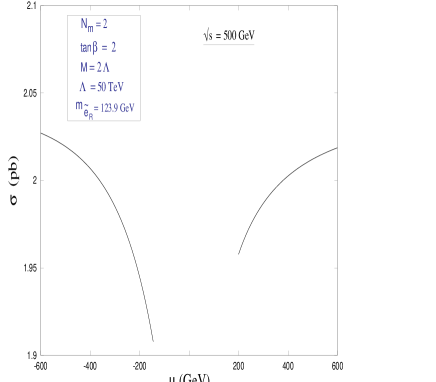
Figure 1: The dependence of $\tilde{e}_{R}$ pair production cross section on the higgsino mass parameter $\mu$. For the assumed set of parameters, the region $|\mu|\mathrel{\hbox to0.0pt{\raise 2.15277pt\hbox{$<$}\hss}{\lower 2.15277pt\hbox{$\sim$}}}200$ GeV has already been ruled out by the existing lower limits on $\widetilde{\chi}^{0}_{1}$ and $\widetilde{\chi}^{+}_{1}$ masses [19].

For a given ratio $\Lambda/M$, both the scalar and the gaugino masses grow with $\Lambda$ (eq. 1). Consequently, the production cross section falls steeply with $\Lambda$ (see Fig. 2$a$). The fall is understandably steeper for larger $N_{m}$ as the selectron mass grows as $\Lambda\sqrt{N_{m}}$. The behaviour for small $\Lambda$ is more subtle. The total cross section is a complicated function of $M_{a}/\sqrt{s}$ and $m_{\widetilde{e}}/\sqrt{s}$. Combined with the fact that the couplings with the $\widetilde{B}$ and $\widetilde{W}_{3}$ are different, this can lead to a situation where the cross sections do not actually fall with $N_{m}$ (Fig. 2$a$). On the other hand, as the mass parameter $M$ enters eq.(1) only logarithmically, one may expect that the cross-sections would change only fractionally as this parameter is varied (for a fixed $\Lambda$). This is borne out by Fig. 2$b$. Since such deviations are almost of the order of statistical fluctuations in the signal itself, for the rest of our study, we will not consider any explicit dependence on the mass ratio $M/\Lambda$.

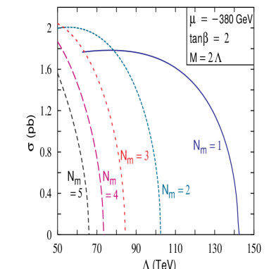
Figure 2: (a) The dependence of $\tilde{e}_{R}$ pair production cross section (for $\sqrt{s}=500\>\rm GeV$) on the scale $\Lambda$ for a fixed ratio of $M/\Lambda$ and given parameters. The intercepts on the $\Lambda$-axis essentially denote the kinematic threshold. For $N_{m}=1$, $\Lambda<60\>\rm GeV$ leads to a spectrum inconsistent with existing lower limits on $\widetilde{\chi}^{0}_{1}$ and $\widetilde{\chi}^{+}_{1}$ masses [19]. (b) The dependence of the cross section on the ratio $M/\Lambda$ for given $\Lambda$.

As we have already pointed out, in GMSB models, the $\tilde{e}_{L}$ is distinctly heavier than the $\tilde{e}_{R}$. Hence, we shall concentrate on the pair-production process $e^{-}e^{-}\rightarrow\tilde{e}_{R}\tilde{e}_{R}$. Once produced, the selectron may decay to either $e^{-}+\tilde{G}$ or $e^{-}+\chi_{1}^{0}$ (if kinematically allowed). In the first case the final state comprises of two electrons and missing momentum, while the second case has two photons in addition. As the backgrounds are quite different, we shall now examine each case individually.

4 Selectron as the NLSP

With the selectrons decaying into an electron and a gravitino each, the SM background comprises of $e^{-}e^{-}\nu_{i}\bar{\nu}_{i}$. The main contributions to the latter clearly arise from the “resonant” processes $e^{-}e^{-}\longrightarrow e^{-}\nu_{e}W^{-}$ and $e^{-}e^{-}\longrightarrow e^{-}e^{-}Z$ and have been discussed at some length in refs. [18, 20]. The $W$ contribution is dominant but can be suppressed by right-polarizing the electron beams. This also serves to enhance the selectron production rate. Of course, the ideal state of a fully polarized beam is virtually unattainable and hereon we shall assume the electron beams to be 90% right-polarized.

It is obvious that the phasespace distribution of the signal events would depend crucially on the mass of the selectron and, to a lesser extent, on the neutralino masses. For purposes of comparison between the signal and the background, we will concentrate on two specific choices in the parameter space marked in Table 1.

	$N_{m}$	$M$	$\Lambda$	$\mu$	$\tan\beta$	$m_{\tilde{e}_{R}}$	$\sigma$ (fb)	$\sigma$ (fb)
		(TeV)	(TeV)	(GeV)		(GeV)	$\sqrt{s}=0.5$ TeV	$\sqrt{s}=1$ TeV
(A)	2	100	50.0	–500	2	123.9	830.3	37.91
	2	120	60.0	400	2	147.3	833.2	43.18
	2	200	100.0	400	3	243.8	202.7	37.99
	3	100	50.0	$-400$	2	149.1	851.5	44.96
	3	150	75.0	350	4	222.8	483.2	42.42
	3	250	62.5	$-350$	4	188.9	705.3	42.41
	4	100	50.0	$-250$	2	170.5	766.5	46.63
	4	250	62.5	450	4	216.2	519.1	43.72
(B)	4	300	60.0	–450	4	208.6	581.7	44.27
	5	100	50.0	$-500$	2	189.6	643.4	46.93
	5	250	62.5	300	3	240.0	214.3	40.52
	5	300	60.0	$-250$	4	231.9	320.2	41.98

Table 1: Signal ($e^{-}e^{-}+p_{T}/\;\>$ ) cross-section for some representative values of GMSB input parameters. The cuts of eqs.(6–9) have been imposed.

Whereas the electrons from an $\tilde{e}_{R}$ would be produced isotropically, the background events would prefer to have at least one of them to be close to the beam pipe [20]. We thus demand that both the electrons must satisfy

$$|\eta_{e}|<3\ ,$$ (6)

a requirement in consistency with the angular coverage of proposed detectors. In addition, the leptons must have sufficient momentum to be detectable, viz

$$p_{T}(e)>5\>\rm GeV\ ,$$ (7)

and be separated enough to be individually resolved:

$$\Delta R\equiv\sqrt{(\Delta\eta)^{2}+(\Delta\phi)^{2}}>0.2\ ,$$ (8)

where $\Delta\phi$ refers to their azimuthal separation. In addition, we demand that the missing momentum be large enough:

$$p_{T}/\;>20\>\rm GeV\ .$$ (9)

With these cuts in place, the total SM background is very flat over the region $\sqrt{s}=500\>\rm GeV$–$1\>\rm TeV$ and amounts to approximately $19.5\>\rm fb$ over the entire range. In Table 1, we display the signal cross-section for some representative values of GMSB parameters. One can get $\sim 10^{4}$ events per year assuming integrated luminosity of $50$ ${\rm fb}^{-1}$ for $\sqrt{s}=500$ GeV and $\sim 10^{3}$ events for $\sqrt{s}=1$ TeV machine (for the same luminosity). In Fig. 3, we present the phasespace distribution for the background events. Also shown in the figure are the corresponding signal profiles for the two particular points in the parameter space. Let us begin by discussing these distributions.

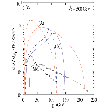
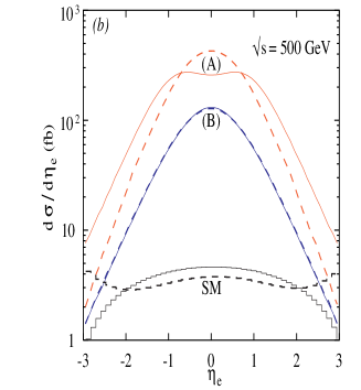
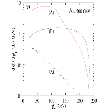
Figure 3: Signal and background distributions for the selectron NLSP case. The histograms correspond to the SM background while the two sets of smooth curves correspond to the signal for parameter sets marked in Table. 1. The cuts of eqs.(6–9) have been imposed. Graph (a) pertains to electron transverse momenta with the solid curves corresponding to the harder electron and the dashed to the softer one. Similarly, graph (b) pertains to the electron rapidities. (c) gives the distribution in missinng transverse momentum.

At first sight, it might seem surprising that the transverse momentum distribution (see Fig. 3$a$) for the signal events do not show the characteristic Jacobian peaks. This is not surprising though, as, for such behaviour to be exhibited, an electron should only appear as a decay product of a particular particle. However, in the case at hand, the two electrons cannot be distinguished from each other and hence have to be ordered in some fashion, whether energy or magnitude of transverse momentum or rapidity. We choose the first option, namely energy ordering. Any such ordering will tend to destroy features indicative of individual decay product kinematics, and this is particularly true of set ($A$). For set ($B$), on the other hand, the selectron mass is much closer to $\sqrt{s}/2$ and hence they are produced with very little momenta. Consequently, the effect of ordering is relatively smaller and the remnant of the Jacobian peak more pronounced.

The rapidity distribution (Fig. 3$b$) for the SM background shows clearly that the softer electron prefers to lie closer to the beam pipe while the harder one is much more central. This is reflective of the singularities in the photon-mediated contributions. This also makes itself felt in the $p_{T}/\;\$ distributions (see Fig. 3$c$) where the SM cross sections fall off much more steeply than those for the signal.

Although the SM background is not too big, it might be desirable to reduce it further without sacrificing a large fraction of the signal. This becomes particularly important when the signal size reduces either on account of $m_{\tilde{e}_{R}}$ being close to the kinematic limit or other (nonstandard) decay modes becoming available to the selectron. A look at Figs. 3 tells clearly that this goal is unlikely to be achieved by imposing harder cuts on either the individual electron $p_{T}$s or on the missing momentum. Removing events with $\eta_{e}>2$ is an option, but even then, the improvement is merely quantitative and not a qualitative one.

In actuality, such a goal is much better realized by examining the double differential cross section rather than making the individual cuts of eqs.(6–9) any stronger. As the $W$-mediated diagrams have been suppressed by right-polarizing the electron beams, the bulk of the background owes its origin to the $e^{-}e^{-}Z$ final state with the $Z$ decaying invisibly. It is easy to see that for such a process, the energies of the two electrons satisfy the conditions [18]

$$\begin{array}[]{rcl}E_{1}+E_{2}&\geq&\displaystyle\frac{s-m_{Z}^{2}}{2\sqrt{s}}\\ (2E_{1}-\sqrt{s})(2E_{2}-\sqrt{s})&\geq&m_{Z}^{2}\ .\end{array}$$ (10)

In Fig. 4$a$, we present a scatter plot of the SM background for an accumulated luminosity of $50\>\rm fb^{-1}$. Superimposed on it are the two curves of eq.(10). Eliminating the part of the phase space bounded by the two curves reduces the SM background from $19\>\rm fb$ to approximately $1fb$. The preponderance of points just below the straight line can be attributed to the contributions from a slightly off-shell $Z$. A very large fraction of these could be eliminated by modifying the straight line curve by replacing $m_{Z}$ with, say, $m_{Z}-2\Gamma_{Z}$. Points well outside this region, on the other hand, owe their origin to the $W$-mediated diagrams and would disappear in the limit of fully right-polarized electron beams.

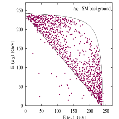
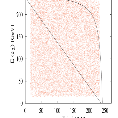
Figure 4: The distribution of the electron energies for the process $e^{-}e^{-}\rightarrow e^{-}e^{-}\nu_{i}\bar{\nu}_{i}$ for $\sqrt{s}=500\>\rm GeV$ and an integrated luminosity of $50\>\rm fb^{-1}$. The cuts of eqs.(6–9) have been imposed. (a) The SM background. Each point corresponds to one event. The events lying in the area enclosed by the straight line and the curve arise from on-shell $Z$ production (see eq.10). (b)The signal events for a particular point in the parameter space. Each point corresponds to four events. The edges of the phase space are given by eqs.(11). Also superimposed are the enclosing curves of (a).

In contrast to the above, the electrons in the signal events are distributed evenly within the square region defined by

$$\begin{array}[]{rcl}\displaystyle E_{\rm min}&\leq&E(e_{i})\leq E_{\rm max}\ ,\\[8.61108pt] E_{\rm min,\ max}&=&\displaystyle\frac{\sqrt{s}}{4}\>\left(1-\frac{m^{2}_{\widetilde{G}}}{m^{2}_{\widetilde{e}}}\right)\;(1\mp\beta)\ ,\\[8.61108pt] \beta&=&\displaystyle\left(1-\frac{4m_{\tilde{e}}^{2}}{s}\right)^{1/2}\ .\end{array}$$ (11)

This is illustrated in Fig. 4$b$. While a significant fraction of the signal cross section could be lost on imposing the cuts corresponding to eq.(10), the signal to noise ratio shows an enormous improvement.

5 Neutralino as the NLSP

As we have already pointed out, for $N_{m}=1$, the lightest neutralino is always the NLSP. Even for $N_{m}>1$, this may continue to be the case especially if the higgsino mass parameter $\mu$ is small. However, in all such cases the gaugino mass parameter $M_{2}$ is larger than the mass of the $\tilde{e}_{R}$. Consequently, the selectron decays mainly into an electron and the lightest neutralino with the latter cascading into a photon and the gravitino. The final state thus comprises of a pair each of electrons and photons and missing energy due to the gravitinos. The energy and angular distributions would obviously depend on the masses of the selectron and the lightest neutralino. We will again concentrate on two representative points (see Table. 2) in our analysis of the signal and comparison with the background.

	$M$	$\Lambda$	$\mu$	$\tan\beta$	$m_{\tilde{e}_{R}}$	$m_{\chi^{0}_{1}}$	$\sigma$ (fb)	$\sigma$ (fb)
	(TeV)	(TeV)	(GeV)		(GeV)	(GeV)	$\sqrt{s}=0.5$ TeV	$\sqrt{s}=1$ TeV
(C)	140	70.0	–450	3	126.6	102.7	1444	277.1
	130	65.0	480	5	119.3	91.35	1372	267.3
	150	75.0	$-300$	6	135.9	108.1	1428	291.3
	160	80.0	400	6	144.2	112.1	1463	308.9
	200	100.0	$-200$	8	178.0	135.4	1378	327.1
	240	80.0	$-200$	9	145.4	107.6	1408	299.3
	230	115.0	250	9	203.7	153.5	1203	331.4
	275	137.5	350	10	242.4	193.2	571	340.0
(D)	500	125.0	450	3	223.1	169.9	1016	343.5

Table 2: Signal ($e^{-}e^{-}+2\gamma+p_{T}/\;\>$ ) cross-section for some representative values of GMSB input parameters. The number of messenger generation $N_{m}=1$. The cuts of eqs.(6–9) and eq.(12) have been imposed.

An exact calculation of the (6-body) SM background is an onerous task. It can be easily seen though that the bulk of the background arises from the two resonant processes:

1. $e^{-}e^{-}\rightarrow e^{-}e^{-}\gamma\gamma Z\rightarrow e^{-}e^{-}\gamma\gamma\nu_{i}\bar{\nu}_{i}$  and

2. $e^{-}e^{-}\rightarrow e^{-}\bar{\nu}_{e}\gamma\gamma W^{-}\rightarrow e^{-}e^{-}\gamma\gamma\nu_{e}\bar{\nu}_{e}$  .

Once soft and collinear singularities have been removed by an appropriate set of cuts, one expects these cross sections to be smaller than those in the previous section by a factor ${\cal O}(\alpha^{2})$. Thus the kinematical cuts required over and above those of eqs.(6–9) are dictated not by the need to minimize background, but by detector acceptances. To be specific, we demand that

$$\begin{array}[]{rclcrcl}|\eta_{\gamma}|&<&3&&p_{T}(\gamma)&>&10\>\rm GeV\\ \Delta R_{\gamma\gamma}&>&0.2&&\Delta R_{e\gamma}&>&0.2\ .\end{array}$$ (12)

With these set of cuts, the surviving cross section, for $\sqrt{s}=500\>\rm GeV$, from process $(i)$ above is approximately $0.004\>\rm fb$ while that from the second one is approximately $0.001\>\rm fb$. Thus, for all practical purposes, we have a background free situation. The surviving size of the signal is quite similar to that in the previous section as the cuts of eq.(12) do not take away much of the signal.

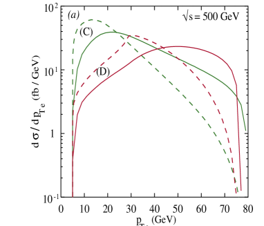
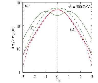
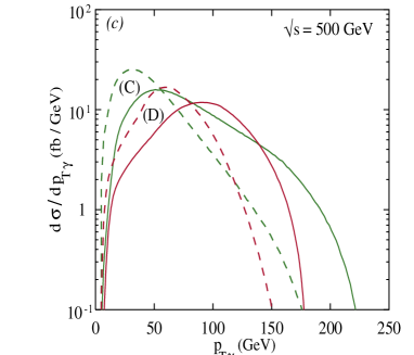
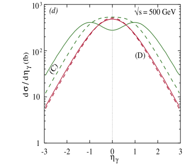
Figure 5: Signal distributions for the neutralino NLSP case. The two sets correspond to parameters marked in Table. 2. The SM background is too small to appear in the graphs as the cuts of eqs.(6–9) and eq.(12) have been imposed. Graph (a) pertains to electron transverse momenta with the solid curves corresponding to the harder electron and the dashed to the softer one. Similarly, graph (b) pertains to the electron rapidity distribution. (c) and (d) respectively give the photon’s transverse momenta and rapidity distributions.

In Fig. 5, we present the signal event distributions for the two particular parameter choices indicated in Table. 2. Comparing Figs. 5$a$ and 3$a$, one is struck by the similarity between the curves for parameter sets ($A$) and ($C$) on the one hand and those for ($B$) and ($D$) on the other. This can be understood by realizing that the shape of electron transverse momenta distribution is determined by the masses of the selectron and the particles it is decaying into. Since cases ($A$) and ($C$) correspond to very similar $m_{\tilde{e}}$, it is only natural that the $p_{T}$ spectrum would look similar. The larger mass of the neutralino (as compared to that for the gravitino) is reflected in smaller value of the maximal $p_{T}$ allowed to the electrons. Analogous statements apply to points ($B$) and ($D$) as well.

We turn now to the photon spectra. As the neutralinos are produced in (isotropic) scalar decays and as they themselves decay into a photon and gravitino, there are no nontrivial angular correlations. Consequently, the spectrum is determined by kinematics alone. This being identical to that for squark decay into massless particles, the decay distributions (Fig. 5$c,d$) are very similar to those for the other set. A similar story obtains for the missing transverse momentum as well.

6 Distinguishing from non-GMSB models

In the last two sections we have seen that, for $\Lambda\>\raisebox{-2.15277pt}{$\stackrel{{\scriptstyle\textstyle<}}{{\sim}}$}\>200\>\rm TeV$, the signal from a GMSB model stands well and truly above the SM background. This is particularly true for the neutralino NLSP case where one expects less than one event from SM processes. This brings us to the more important question, namely how to recognize if supersymmetry breaking is driven by gauge mediation. It goes without saying, though, that short of determining the entire spectrum, one can only draw (strong) inferences and this is what we shall aim to do in this section.

Considering the selectron NLSP case first, it is clear that eq.(11) can be used to determine the masses of both the selectron and the supersymmetric particle $X$ (gravitino or neutralino) that it is decaying into. Of course, measurement of the edge of phasespace is always beset with inaccuracies. However, at this stage we do not need to know the mass of $X$ very accurately. In fact, as long as the experimentally deduced value $m_{X}\>\raisebox{-2.15277pt}{$\stackrel{{\scriptstyle\textstyle<}}{{\sim}}$}\>30\>\rm GeV$ or so, the rest of argument follows. LEP data already tells us that such a light neutralino can only be the bino (primarily). Now, the $\tilde{e}_{R}$ does not couple with the $\tilde{W}_{3}$ and its coupling with the higgsinos is suppressed by the electron mass. Consequently, for a $\tilde{e}_{R}$ of fixed mass, the production cross section (eq.5) is determined essentially by the bino mass $M_{1}$. Working in the limit $M_{2},\mu\gg M_{1}$, the chirality structure of the amplitude ensures that, for small values of $M_{1}^{2}/s$, the cross section grows as this ratio (see Fig. 6). For large values of the ratio, though, the cross section would fall off. Realistic values for $M_{2}$ and $\mu$ would alter our simplistic arguments to a degree, but such effects are too small to be noticeable in the graph that we present.

Figure 6: The variation of $\tilde{e}_{R}$ pair production cross section with the gaugino mass parameter $M_{1}$. No assumption regarding SUSY breaking has been made. The dependence on $M_{2}$, $\mu$ and $\tan\beta$ is negligible.

That we have produced a pair of $\tilde{e}_{R}$s and not $\tilde{e}_{L}$s we can deduce from the polarization of the initial state. Its mass, as we have already seen, can be determined from the energy distribution, and if necessary, refined by a threshold scan. At this stage, Fig. 6 can be used to “determine” $M_{1}$ from the experimentally measured cross section and compare it with the direct, if inaccurate, measurement from the endpoint analysis. Clearly, the consistency between the two values would be much higher for the GMSB hypothsis than for the non-GMSB case. Thus, rate counting helps us to to distinguish between the light gravitino and light bino cases.

The neutralino NLSP case presents us with an additional complication. Presumably we could have had $\tilde{e}_{R}\rightarrow e^{-}+\chi_{2}^{0}$ in a non-GMSB scenario followed by $\chi_{2}^{0}\rightarrow\chi_{1}^{0}+\gamma$. We can again measure both $m_{\tilde{e}_{R}}$ and $m_{\chi}$ by determining the phasespace boundaries of the electrons and employing a relation analogous to eq.(11). What about the mass of the gravitino (neutralino) in the second stage of the decay? In fact, a corresponding relation can be derived for the energy of the photons:

$$\begin{array}[]{rcl}E_{\gamma}^{\rm max,min}&=&\displaystyle A\>(1\pm\beta)\>(1\pm\zeta)\\[8.61108pt] A&\equiv&\displaystyle\frac{\sqrt{s}}{8}\left(1+\frac{m_{\chi}^{2}}{m^{2}_{\widetilde{e}}}\right)\>\left(1-\frac{m^{2}_{\tilde{G}}}{m_{\chi}^{2}}\right)\\[8.61108pt] \zeta&\equiv&\displaystyle\frac{m_{\chi}^{2}-m^{2}_{\tilde{G}}}{m_{\chi}^{2}+m^{2}_{\tilde{G}}}\ ,\end{array}$$ (13)

with $\beta$ defined as in eq.(11).

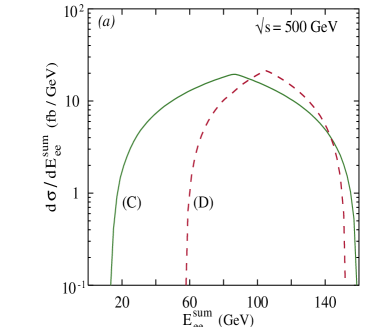
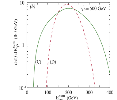
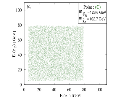
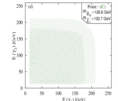
Figure 7: (a) The distribution in the scalar sum of the electron energies for the signal events in the neutralino NLSP case. The cuts of eqs.(6–9) and eq.(12) have been imposed. The legends refer to the parameter set marked in Table. 2. THE SM background is too small to appear on the graph. (b) Similar distribution but in the scalar sum of photon energies. (c) Scatter plot in the electron energies for an integrated luminosity of $50\>\rm fb^{-1}$. Each point corresponds to four events. (d) Similar scatter plot in the photon energies.

In Figs. 7($a,b$), we exhibit the distributions in the scalar sums of electron and photon energies respectively. The first, namely $E_{ee}^{\rm sum}\equiv E_{e_{1}}+E_{e_{2}}$, leads to a symmetric distribution as in the case of a selectron NLSP. On the other hand, the distribution in $E_{\gamma\gamma}^{\rm sum}$ shows a high energy tail. The tail is purely a kinematic feature and can be derived from a generalization of the Dalitz plot. A better understanding of the same can be obtained from the scatter plots of Figs. 7($c,d$).

As in the previous case, the endpoints of the electron spectrum can be used to deduce both $m_{\tilde{e}_{R}}$ and $m_{\chi}$. Once $m_{\tilde{e}_{R}}$ is measured, eq.(13) can be used to determine both $m_{\chi}$ and $m_{\tilde{G}}$. This, thus, also serves as a consistency check. At this stage we can again take recourse to Fig. 6 to argue that the existence of such a light bino (as in a non-GMSB model) would have implied a small cross section. Moreover, if such a bino were to exist, the selectron would have a substantial branching into it. Hence, nonobservance of an excess in the ($e^{-}e^{-}+$ missing energy) final state is yet another argument against a spectrum with a heavy gravitino but a light bino.

7 Summary

The $e^{-}e^{-}$ option of the Next Generation Linear collider can be a very effective tool in the search for physics beyond the SM. In this paper, we have studied the feasibility of using such a machine to probe Gauge Mediated Supersymmetry Breaking. The process of choice is the pair-production of right-handed selectrons, not in the least because of their being significantly lighter than their left-handed counterparts.

If the selectron be the NLSP, the signal comprises two electrons accompanied by a missing momentum. Right-polarizing (90%) the electron beams helps eliminate the bulk of the SM background apart from increasing the signal strength as well. The already very good signal to noise ratio can be enhanced even further by imposing correlated cuts on the electron energies. The neutralino NLSP case, on the other hand results in a spectacular final state comprising a pair each of electrons and photons accompanied by missing momentum. The SM background is virtually nonexistent. In either case, the rates are high enough for the selectron to be detectible almost upto the kinematic limit.

The energy correlations (electrons for the selectron NLSP case and both electrons and photons in the neutralino NLSP case) are characteristic and can be used to determine the masses of both the produced particle and its decay products. Furthermore, such information gleaned from the differential distributions, used in conjunction with rate counts, can be used to distingguish GMSB from alternate scenarios of supersymmetry breaking (including, but not limited to, the case of supergravity-inspired models without gaugino mass unification).

Acknowledgement

DC acknowledges the Department of Science and Technology, India for the Swarnajayanti Fellowship grant. DKG acknowledges the hospitality of the Theory Divison, CERN, Geneva and the Laboratorie de Physique Particles (LAPP), Annecy, where a part of this work was done.

References

- [1] S. Ferrara, L. Girardello and F. Palumbo, Phys. Rev. D20 (1979) 403.
-
[2]
See, e.g., H.P. Nilles, Phys. Rep. 110 (1984) 1;
H.E. Haber and G.L. Kane, Phys. Rep. 117 (1985) 75;
A. Chamseddine, R. Arnowitt and P. Nath, Applied Supergravity, World Scientific, Singapore (1984);
G.L. Kane, hep-ph/9709318. - [3] R. Barbieri, L. Hall and A. Strumia, Nucl. Phys. B455 (1995) 219.
-
[4]
M. Dine, W. Fischler and M. Srednicki, Nucl. Phys. B189 (1981) 575;
S. Dimopoulos and S. Raby, Nucl. Phys. B192 (1981) 353;
M. Dine and W. Fischler, Phys. Lett. B110 (1982) 227;
M. Dine and M. Srednicki, Nucl. Phys. B202 (1982) 238;
C. Nappi and B. Ovrut, Phys. Lett. B113 (1982) 175. -
[5]
M. Dine and W. Fischler, Nucl. Phys. B204 (1982) 346;
L. Alvarez-Gaumé, M. Claudson and M.B. Wise, Nucl. Phys. B207 (1982) 96;
S. Dimopoulos and S. Raby, Nucl. Phys. B219 (1983) 479. -
[6]
M. Dine, A.E. Nelson and Y. Shirman, Phys. Rev. D51 (1995) 1362;
M. Dine, A. Nelson, Y. Nir and Y. Shirman, Phys. Rev. D53 (1996) 2658;
M. Dine, Y. Nir and Y. Shirman, Phys. Rev. D55 (1997) 1501. -
[7]
S. Dimopoulos and G.F. Giudice, Phys. Lett. B393 (1997) 72;
G. Dvali and M. Shifman, Phys. Lett. B399 (1997) 60;
M. Hotta, K.-I. Izawa and T. Yanagida, Phys. Rev. D55 (1997) 415;
S.P. Martin, Phys. Rev. D55 (1997) 3177;
L. Randall, hep-ph/9612426;
J. Bagger et al., Phys. Rev. Lett. 78 (1997) 1002, (E) ibid 78 (1997) 2497; Phys. Rev. D55 (1997) 3188;
S. Dimopoulos, S. Thomas and J.D. Wells, Nucl. Phys. B488 (1997) 39. -
[8]
A. Riotto, O. Törnkvist and R.N. Mohapatra,
Phys. Lett. B388 (1996) 599;
N. Arkani-Hamed, J. March-Russell and H. Murayama, Nucl. Phys. B509 (1998) 3;
F. Borzumati, hep-ph/9702307. - [9] For a recent review, see G.F. Giudice and A. Rattazzi, Phys. Rep. 322 (1999) 419.
-
[10]
L. Randall and R. Sundrum, Nucl. Phys. B557 (1999) 79;
G. F. Giudice, et al., JHEP 9812 (1998) 027;
J. A. Bagger, T. Moroi, and E. Poppitz, JHEP 0004 (2000) 009;
J. L. Feng and T. Moroi, Phys. Rev. D61 (2000) 095004. -
[11]
T. Gherghetta et al., Nucl. Phys. B559 (1999) 27;
S. Su, Nucl. Phys. B573 (2000) 87;
J . L. Feng et al., Phys. Rev. Lett. 83 (1999) 1731;
F. Paige and J. Wells, hep-ph/0001249;
D.K. Ghosh, P.Roy and S. Roy, hep-ph/0004127;
U. Chattopadhyay, D.K. Ghosh and S. Roy, hep-ph/0006049. -
[12]
S. Dimopoulos, M. Dine, S. Raby and S. Thomas,
Phys. Rev. Lett. 76 (1996) 3494;
S. Ambrosanio et al., Phys. Rev. Lett. 76 (1996) 3498; Phys. Rev. D54 (1996) 5395;
K.S. Babu, C. Kolda and F. Wilczek, Phys. Rev. Lett. 77 (1996) 3070. -
[13]
S. Dimopoulos, S. Thomas and J.D. Wells,
Phys. Rev. D54 (1996) 3283;
H. Baer, M. Brhlik, C. Chen and X. Tata, Phys. Rev. D55 (1997) 4463;
H. Baer, P.G. Mercadante, X. Tata and Y. Wang, hep-ph/0004001. -
[14]
J.L. Lopez, D.V. Nanopoulos and A. Zichichi,
Phys. Rev. Lett. 77 (1996) 5168; Phys. Rev. D55 (1997) 5813;
D.A. Dicus, B. Dutta and S. Nandi, Phys. Rev. Lett. 78 (1997) 3055;
S. Ambrosanio, G.D. Kribs and S.P. Martin, Phys. Rev. D56 (1997) 1761. -
[15]
D. Stump, M. Wiest and C.-P. Yuan, Phys. Rev. D54 (1996) 1936;
A. Ghosal, A. Kundu and B. Mukhopadhyaya, Phys. Rev. D56 (1997) 504;
A. Datta et al., Phys. Lett. B416 (1998) 117. - [16] B. Mukhopadhyaya, and S. Roy, Phys. Rev. D57 (1998) 6793.
- [17] W.-Y. Keung and L. Littenberg, Phys. Rev. D28 (1983) 1067.
- [18] F. Cuypers, G.J. van Oldenborgh and R. Rückl, Nucl. Phys. B409 (1993) 128.
-
[19]
B. Abbott et al.(D0 Collab.) Phys. Rev. Lett. 80 (1998) 442;
R. Barate et al.(ALEPH Collab.), CERN preprint CERN-EP/99-171. - [20] D. Choudhury and F. Cuypers, Phys. Lett. B325 (1994) 500; Nucl. Phys. B429 (33) 1994.