Longitudinal Resolution in a Large Relativistic Nucleus:
Adding a Dimension to the McLerran-Venugopalan Model

Abstract

We extend the McLerran-Venugopalan model for the gluon distribution functions of very large nuclei to larger values of the longitudinal momentum fraction $x_{{}_{F}}$. Because gluons with larger values of $x_{{}_{F}}$ begin to resolve the longitudinal structure of the nucleus, we find that it is necessary to set up a fully three-dimensional formalism for performing the calculation. We obtain a relatively compact expression for the gluon number density provided that the nucleus is sufficiently large and consists of color-neutral nucleons. Our expressions for the gluon number density saturate at small transverse momenta. The nuclear dependence we obtain is such that the number of gluons increases more slowly than the number of nucleons is increased.

I Introduction

The recent construction and commissioning of the Brookhaven Relativistic Heavy Ion Collider has led to a renewed interest in the properties of heavy nuclei in recent years. A considerable amount of fruitful work has been done on classical and semiclassical descriptions of the physics involved[3, 4, 5, 6, 7, 8, 9, 10, 11, 12, 13, 14, 15, 16, 17, 18, 19, 20, 21]. In particular, the McLerran-Venugopalan (MV) model[3, 4, 5, 6, 7] provides a framework for calculating the gluon distribution functions for very large nuclei at very small values of the longitudinal momentum fraction $x_{{}_{F}}$. What McLerran and Venugopalan realized is that at sufficiently small $x_{{}_{F}}$, the gluons are unable to resolve the longitudinal structure of the nucleus, meaning that many quarks contribute to the color field at each value of the (transverse) position $\textstyle x$. This large charge per unit area $\kappa^{2}$ provides the scale at which the strong coupling is evaluated[3]. Thus, if $\kappa^{2}\gg\Lambda_{\rm QCD}^{2}$, a classical treatment ought to provide a reasonable description.

Recently, we pointed out that the infrared divergences which appear in the MV model may be cured by incorporating the effects of confinement[8]. That is, we observe that nucleons display no net color charge: individual quarks are confined inside the nucleons, whose radius is $a\sim\Lambda_{\rm QCD}^{-1}$. As a consequence, we expect that there should not be long range ($\gg a$) correlations between quarks. Strong correlations between quarks occur only when we probe at short distance scales. These considerations may be phrased as a mathematical constraint on the form of the two-point charge density correlation function.

The calculations presented in Refs. [3, 4, 5, 6, 7, 8] all assume $x_{{}_{F}}$ to be small enough so that the gluons do not probe the longitudinal structure of the Lorentz-contracted nucleus which they see. Effectively, then, the relevant geometry is two-dimensional, with the source exactly on the light cone. In this work we extend the MV model to larger values of the longitudinal momentum fraction $x_{{}_{F}}$. In this regime, the gluons begin to resolve the longitudinal structure of the nucleus: therefore, we develop a fully three-dimensional framework using a source that is not quite aligned with the light cone. In order to deal with the complications which arise as a result, we must rely heavily on the fact that we consider a large nucleus of radius $R\gg a$ which consists of color-neutral nucleons.

The remainder of this paper is organized as follows. In Sec. II we present our conventions for writing down the classical Yang-Mills equations and describe the (slightly) off-light-cone source which will be the foundation of our calculation. We show that the natural (order unity) variables to describe the nucleus are essentially those in the nuclear rest frame, even in the limit $\beta\rightarrow 1$. In Sec. III we set up the framework for determining the gluon number density in the Weizsäcker-Williams approximation. In this section we introduce the two-point charge density correlation function, and review the color-neutrality condition[8] which it must satisfy. Sec. IV contains a discussion of the requirements which must be satisfied in order for our approximations to be valid. The meat of our calculation is contained in Sec. V, where we begin with the solution for the vector potential in the covariant gauge, perform the transformation to light-cone gauge, and determine the gluon number density. Additional details of this calculation are found in Appendix A. We illustrate our results for the gluon number density with the help of a power-law model for the correlation function in Sec. VI. The integrals which arise in connection with this model are presented in Appendix B. Finally, Sec. VII contains our conclusions.

II The Classical Yang-Mills Equations and Source

In this section we present the conventions which we use in writing down the Yang-Mills equations and source for a nucleus which moves down the $z$ axis with a speed $\beta<1$. The motivation behind the choices we have made is to ensure that all “unknown” quantities are of order unity, with all powers of the small and large parameters explicitly written out. This will make the approximations which we will have to make later on more transparent. It will also make the $\beta\rightarrow 1$ limit which we take at the end obvious.

We begin with the classical Yang-Mills equations, which we write as

$$D_{\mu}F^{\mu\nu}=gJ^{\nu},$$ (1)

where we have employed matrix form, i.e. $J^{\nu}\equiv T^{a}J^{a\nu}$, etc. The $T^{a}$ are the normalized Hermitian generators of SU($N_{c}$) in the fundamental representation, satisfying $2\thinspace{\rm Tr}(T^{a}T^{b})=\delta^{ab}$. The covariant derivative is

$$D_{\mu}F^{\mu\nu}\equiv\partial_{\mu}F^{\mu\nu}-ig\mathchoice{{\hbox{\boldmath$\displaystyle\Bigl{[}$}}}{{\hbox{\boldmath$\textstyle\Bigl{[}$}}}{{\hbox{\boldmath$\scriptstyle\Bigl{[}$}}}{{\hbox{\boldmath$\scriptscriptstyle\Bigl{[}$}}}A_{\mu},F^{\mu\nu}\mathchoice{{\hbox{\boldmath$\displaystyle\Bigr{]}$}}}{{\hbox{\boldmath$\textstyle\Bigr{]}$}}}{{\hbox{\boldmath$\scriptstyle\Bigr{]}$}}}{{\hbox{\boldmath$\scriptscriptstyle\Bigr{]}$}}}$$ (2)

and the field strength reads

$$F^{\mu\nu}\equiv\partial^{\mu}A^{\nu}-\partial^{\nu}A^{\mu}-ig\mathchoice{{\hbox{\boldmath$\displaystyle\Bigl{[}$}}}{{\hbox{\boldmath$\textstyle\Bigl{[}$}}}{{\hbox{\boldmath$\scriptstyle\Bigl{[}$}}}{{\hbox{\boldmath$\scriptscriptstyle\Bigl{[}$}}}A^{\mu},A^{\nu}\mathchoice{{\hbox{\boldmath$\displaystyle\Bigr{]}$}}}{{\hbox{\boldmath$\textstyle\Bigr{]}$}}}{{\hbox{\boldmath$\scriptstyle\Bigr{]}$}}}{{\hbox{\boldmath$\scriptscriptstyle\Bigr{]}$}}}.$$ (3)

The conventions contained in Eqs. (1)–(3) ensure that all powers of the strong coupling constant $g$ are explicit, with no hidden $g$-dependence.

We now turn to the source appearing in (1), starting in the rest frame of the nucleus. Using the subscript “$r$” to denote rest frame quantities, the current takes on the simple form

$$J_{r}^{0}=\rho(-z_{r},\mathchoice{{\hbox{\boldmath$\displaystyle x$}}}{{\hbox{\boldmath$\textstyle x$}}}{{\hbox{\boldmath$\scriptstyle x$}}}{{\hbox{\boldmath$\scriptscriptstyle x$}}}_{r});\qquad J_{r}^{1}=J_{r}^{2}=J_{r}^{3}=0.$$ (4)

The color charge density $\rho\equiv T^{a}\rho^{a}$ is a spherically symmetric function which is non-zero over a region of size $R$, the radius of the nucleus. Since in the lab frame we want the nucleus to be moving along the $+z$ axis, it is convenient to use $-z_{r}$ for the longitudinal coordinate in Eq. (4). The transverse coordinates $x_{r}$ and $y_{r}$ form a two-vector which we write in bold-face: $\mathchoice{{\hbox{\boldmath$\displaystyle x$}}}{{\hbox{\boldmath$\textstyle x$}}}{{\hbox{\boldmath$\scriptstyle x$}}}{{\hbox{\boldmath$\scriptscriptstyle x$}}}_{r}$. In terms of the light-cone coordinates $x^{\pm}=-x_{\mp}=(x^{0}\pm x^{3})/\sqrt{2},$ Eq. (4) may be written as

$$J^{+}_{r}=J^{-}_{r}=\hbox{${1}\over{\sqrt{2}}$}\rho\Bigl{(}\hbox{${1}\over{\sqrt{2}}$}(x^{-}_{r}{-}x^{+}_{r}),\mathchoice{{\hbox{\boldmath$\displaystyle x$}}}{{\hbox{\boldmath$\textstyle x$}}}{{\hbox{\boldmath$\scriptstyle x$}}}{{\hbox{\boldmath$\scriptscriptstyle x$}}}_{r}\Bigr{)};\qquad\mathchoice{{\hbox{\boldmath$\displaystyle J$}}}{{\hbox{\boldmath$\textstyle J$}}}{{\hbox{\boldmath$\scriptstyle J$}}}{{\hbox{\boldmath$\scriptscriptstyle J$}}}_{r}={\bf 0}.$$ (5)

The net color charge of the nucleus is zero:

$$\int dz_{r}\thinspace d^{2}\mathchoice{{\hbox{\boldmath$\displaystyle x$}}}{{\hbox{\boldmath$\textstyle x$}}}{{\hbox{\boldmath$\scriptstyle x$}}}{{\hbox{\boldmath$\scriptscriptstyle x$}}}_{r}\thinspace\thinspace\rho(-z_{r},\mathchoice{{\hbox{\boldmath$\displaystyle x$}}}{{\hbox{\boldmath$\textstyle x$}}}{{\hbox{\boldmath$\scriptstyle x$}}}{{\hbox{\boldmath$\scriptscriptstyle x$}}}_{r})=0.$$ (6)

The nucleus is not a homogeneous sphere of color charge: it has substructure. Because of confinement, there are smaller regions of size $a\sim\Lambda_{\rm QCD}^{-1}$ within the volume occupied by the nucleus for which the total color charge also vanishes. These regions correspond to the nucleons. For a large nucleus, $a/R\approx A^{-1/3}\ll 1$.

Boosting to the lab frame, where the nucleus moves along the $+z$ axis with a speed $\beta$, Eq. (5) becomes

$$J^{+}={{1}\over{\varepsilon}}\thinspace\rho\Bigl{(}\hbox{${{1}\over{\varepsilon}}$}x^{-}{-}\hbox{${{\varepsilon}\over{2}}$}x^{+},\mathchoice{{\hbox{\boldmath$\displaystyle x$}}}{{\hbox{\boldmath$\textstyle x$}}}{{\hbox{\boldmath$\scriptstyle x$}}}{{\hbox{\boldmath$\scriptscriptstyle x$}}}\Bigr{)};\qquad J^{-}={{\varepsilon}\over{2}}J^{+};\qquad\mathchoice{{\hbox{\boldmath$\displaystyle J$}}}{{\hbox{\boldmath$\textstyle J$}}}{{\hbox{\boldmath$\scriptstyle J$}}}{{\hbox{\boldmath$\scriptscriptstyle J$}}}={\bf 0},$$ (7)

where we have defined

$$\varepsilon\equiv\sqrt{{{2(1-\beta)}\over{1+\beta}}}.$$ (8)

Viewed in the lab frame, the nucleus is Lorentz-contracted to a thickness of order $R/\gamma$, where, as usual, $\gamma\equiv(1{-}\beta^{2})^{-1/2}$. For large boosts the charge density function is non-zero only when $x^{-}\sim\varepsilon R$. Hence, the longitudinal argument in Eq. (7) is really of order $R$, leading us to define the new longitudinal variable

$$x_{\scriptscriptstyle\parallel}\equiv{{1}\over{\varepsilon}}\thinspace x^{-}-{{\varepsilon}\over{2}}\thinspace x^{+}.$$ (9)

The current appearing in Eq. (7) is a function of $(x_{\scriptscriptstyle\parallel},\mathchoice{{\hbox{\boldmath$\displaystyle x$}}}{{\hbox{\boldmath$\textstyle x$}}}{{\hbox{\boldmath$\scriptstyle x$}}}{{\hbox{\boldmath$\scriptscriptstyle x$}}})\equiv\vec{x}$. The use of the notation “$\vec{x}$ ” is suggestive of the fact that, in terms of the natural (order unity) variables, the functions describing the nucleus are still spherical! In fact, $x_{\scriptscriptstyle\parallel}$ is just the (unboosted) longitudinal coordinate from the rest frame. The advantage of using $x_{\scriptscriptstyle\parallel}$ instead of $x^{-}$ should be obvious: to take the $\beta\rightarrow 1$ ($\varepsilon\rightarrow 0$) limit for quantities written in terms of $x_{\scriptscriptstyle\parallel}$ is trivial, whereas if the same quantities were written in terms of $x^{-}$ instead, we would have to be careful to hold $x^{-}/\varepsilon$ fixed.

Because the choice made in (4), we define

$$\vec{q}\cdot\vec{x}\equiv-q_{\scriptscriptstyle\parallel}x_{\scriptscriptstyle\parallel}+\mathchoice{{\hbox{\boldmath$\displaystyle q$}}}{{\hbox{\boldmath$\textstyle q$}}}{{\hbox{\boldmath$\scriptstyle q$}}}{{\hbox{\boldmath$\scriptscriptstyle q$}}}\cdot\mathchoice{{\hbox{\boldmath$\displaystyle x$}}}{{\hbox{\boldmath$\textstyle x$}}}{{\hbox{\boldmath$\scriptstyle x$}}}{{\hbox{\boldmath$\scriptscriptstyle x$}}}.$$ (10)

We will also use the notation $d^{3}\vec{x}\equiv dx_{\scriptscriptstyle\parallel}\thinspace d^{2}\mathchoice{{\hbox{\boldmath$\displaystyle x$}}}{{\hbox{\boldmath$\textstyle x$}}}{{\hbox{\boldmath$\scriptstyle x$}}}{{\hbox{\boldmath$\scriptscriptstyle x$}}}$. All of the functions we will be dealing with will depend only on the particular combination of $x^{+}$ and $x^{-}$ appearing in Eq. (9). Thus, we have the replacements

$$\partial_{+}\rightarrow-{{\varepsilon}\over{2}}\thinspace{{\partial}\over{\partial x_{\scriptscriptstyle\parallel}}}\equiv-{{\varepsilon}\over{2}}\thinspace\partial_{\scriptscriptstyle\parallel};\qquad\partial_{-}\rightarrow{{1}\over{\varepsilon}}\thinspace\partial_{\scriptscriptstyle\parallel}.$$ (11)

The divergence of the current in Eq. (7) vanishes: $\partial_{\mu}J^{\mu}=0$. In QCD, however, we require that the current be covariantly conserved: $D_{\mu}J^{\mu}=0$. Since we are at weak coupling, we may work iteratively. That is, we first solve the Yang-Mills equations using (7) for the source. The resulting solution will violate the covariant conservation condition by an amount of order $g^{2}$. The value of $D_{\mu}J^{\mu}$ which is obtained could, in principle, be used to correct the current to this order given the non-Abelian equivalent of the Lorentz force equation to provide information on how the color of the quarks making up the source changes upon emission of a gluon. Since we are assuming that $g^{2}\ll 1$, we will simply drop these contributions.

As suggested by Eq. (10), we will use the notation $q_{\scriptscriptstyle\parallel}$ for the component of momentum conjugate to $x_{\scriptscriptstyle\parallel}$. To make the connection with the longitudinal momentum fraction $x_{{}_{F}}$, let the gluon carry a momentum $q^{+}$ and the nucleon a momentum $Q^{+}$. Then,

$$x_{{}_{F}}\equiv{{q^{+}}\over{Q^{+}}}={{\varepsilon q^{+}}\over{m}},$$ (12)

where $m$ is the nucleon mass. However,

$$q^{+}\leftrightarrow i\partial_{-}\leftrightarrow{{i}\over{\varepsilon}}\thinspace\partial_{\scriptscriptstyle\parallel}\leftrightarrow{{q_{\scriptscriptstyle\parallel}}\over{\varepsilon}}.$$ (13)

Thus, we conclude that

$$x_{{}_{F}}\equiv{{q_{\scriptscriptstyle\parallel}}\over{m}}.$$ (14)

Once more note the advantage of the rest-frame variables over the light-cone variables: in terms of $q^{+}$, we would have to take the $\varepsilon\rightarrow 0$ limit with the caveat that the combination $\varepsilon q^{+}$ is held fixed. No such complication arises when we use $q_{\scriptscriptstyle\parallel}$ instead.

III Counting Gluons

Next, we turn to the formula for the gluon number density. Recall that the standard expression reads[22]

$${{dN}\over{dq^{+}d^{2}\mathchoice{{\hbox{\boldmath$\displaystyle q$}}}{{\hbox{\boldmath$\textstyle q$}}}{{\hbox{\boldmath$\scriptstyle q$}}}{{\hbox{\boldmath$\scriptscriptstyle q$}}}}}={{q^{+}}\over{4\pi^{3}}}\negthinspace\int_{-\infty}^{\infty}\negthinspace dx^{-}\int_{-\infty}^{\infty}\negthinspace dx^{\prime-}\int d^{2}\mathchoice{{\hbox{\boldmath$\displaystyle x$}}}{{\hbox{\boldmath$\textstyle x$}}}{{\hbox{\boldmath$\scriptstyle x$}}}{{\hbox{\boldmath$\scriptscriptstyle x$}}}\int d^{2}\mathchoice{{\hbox{\boldmath$\displaystyle x$}}}{{\hbox{\boldmath$\textstyle x$}}}{{\hbox{\boldmath$\scriptstyle x$}}}{{\hbox{\boldmath$\scriptscriptstyle x$}}}^{\prime}\thinspace e^{-iq^{+}(x^{-}-x^{\prime-})}e^{i\mathchoice{{\hbox{\boldmath$\displaystyle q$}}}{{\hbox{\boldmath$\textstyle q$}}}{{\hbox{\boldmath$\scriptstyle q$}}}{{\hbox{\boldmath$\scriptscriptstyle q$}}}\cdot(\mathchoice{{\hbox{\boldmath$\displaystyle x$}}}{{\hbox{\boldmath$\textstyle x$}}}{{\hbox{\boldmath$\scriptstyle x$}}}{{\hbox{\boldmath$\scriptscriptstyle x$}}}-\mathchoice{{\hbox{\boldmath$\displaystyle x$}}}{{\hbox{\boldmath$\textstyle x$}}}{{\hbox{\boldmath$\scriptstyle x$}}}{{\hbox{\boldmath$\scriptscriptstyle x$}}}^{\prime})}\langle A_{i}^{a}(x^{-},\mathchoice{{\hbox{\boldmath$\displaystyle x$}}}{{\hbox{\boldmath$\textstyle x$}}}{{\hbox{\boldmath$\scriptstyle x$}}}{{\hbox{\boldmath$\scriptscriptstyle x$}}})A_{i}^{a}(x^{\prime-},\mathchoice{{\hbox{\boldmath$\displaystyle x$}}}{{\hbox{\boldmath$\textstyle x$}}}{{\hbox{\boldmath$\scriptstyle x$}}}{{\hbox{\boldmath$\scriptscriptstyle x$}}}^{\prime})\rangle.$$ (15)

Eq. (15) is written in terms of the light-cone variables $x^{-}$ and $q^{+}$, and the light-cone gauge vector potential $A_{i}$. The light-cone gauge has favored status with respect to the intuitive picture of the parton model[22, 23, 24, 25]: thus we continue to use the light-cone gauge even for a source which moves at less than the speed of light. Based on the discussion of Sec. II, however, we wish to employ the “new” longitudinal variables $x_{\scriptscriptstyle\parallel}$ and $q_{\scriptscriptstyle\parallel}$; therefore, we write

$${{dN}\over{dq_{\scriptscriptstyle\parallel}d^{2}\mathchoice{{\hbox{\boldmath$\displaystyle q$}}}{{\hbox{\boldmath$\textstyle q$}}}{{\hbox{\boldmath$\scriptstyle q$}}}{{\hbox{\boldmath$\scriptscriptstyle q$}}}}} \equiv {{q_{\scriptscriptstyle\parallel}}\over{4\pi^{3}}}\thinspace\int d^{3}\vec{x}\int d^{3}\vec{x}\thinspace^{\prime}\thinspace e^{i\vec{q}\cdot(\vec{x}-\vec{x}\thinspace^{\prime})}\langle A_{i}^{a}(\vec{x}\thinspace)A_{i}^{a}(\vec{x}\thinspace^{\prime})\rangle\negthinspace\negthinspace\negthinspace\negthinspace$$ (16)

$$= {{q_{\scriptscriptstyle\parallel}}\over{4\pi^{3}}}\thinspace\int d^{2}\mathchoice{{\hbox{\boldmath$\displaystyle x$}}}{{\hbox{\boldmath$\textstyle x$}}}{{\hbox{\boldmath$\scriptstyle x$}}}{{\hbox{\boldmath$\scriptscriptstyle x$}}}\int d^{2}\mathchoice{{\hbox{\boldmath$\displaystyle x$}}}{{\hbox{\boldmath$\textstyle x$}}}{{\hbox{\boldmath$\scriptstyle x$}}}{{\hbox{\boldmath$\scriptscriptstyle x$}}}^{\prime}\thinspace e^{i\mathchoice{{\hbox{\boldmath$\displaystyle q$}}}{{\hbox{\boldmath$\textstyle q$}}}{{\hbox{\boldmath$\scriptstyle q$}}}{{\hbox{\boldmath$\scriptscriptstyle q$}}}\cdot(\mathchoice{{\hbox{\boldmath$\displaystyle x$}}}{{\hbox{\boldmath$\textstyle x$}}}{{\hbox{\boldmath$\scriptstyle x$}}}{{\hbox{\boldmath$\scriptscriptstyle x$}}}-\mathchoice{{\hbox{\boldmath$\displaystyle x$}}}{{\hbox{\boldmath$\textstyle x$}}}{{\hbox{\boldmath$\scriptstyle x$}}}{{\hbox{\boldmath$\scriptscriptstyle x$}}}^{\prime})}\langle A_{i}^{a}(q_{\scriptscriptstyle\parallel};\mathchoice{{\hbox{\boldmath$\displaystyle x$}}}{{\hbox{\boldmath$\textstyle x$}}}{{\hbox{\boldmath$\scriptstyle x$}}}{{\hbox{\boldmath$\scriptscriptstyle x$}}})A_{i}^{a}(-q_{\scriptscriptstyle\parallel};\mathchoice{{\hbox{\boldmath$\displaystyle x$}}}{{\hbox{\boldmath$\textstyle x$}}}{{\hbox{\boldmath$\scriptstyle x$}}}{{\hbox{\boldmath$\scriptscriptstyle x$}}}^{\prime})\rangle,$$ (17)

where

$$A(q_{\scriptscriptstyle\parallel};\mathchoice{{\hbox{\boldmath$\displaystyle x$}}}{{\hbox{\boldmath$\textstyle x$}}}{{\hbox{\boldmath$\scriptstyle x$}}}{{\hbox{\boldmath$\scriptscriptstyle x$}}})\equiv\int_{-\infty}^{\infty}dx_{\scriptscriptstyle\parallel}\thinspace e^{-iq_{\scriptscriptstyle\parallel}x_{\scriptscriptstyle\parallel}}\thinspace A(\vec{x}\thinspace).$$ (18)

In the limit $\varepsilon\rightarrow 0$, Eq. (17) reduces to the previous result, Eq. (15).

Eq. (17) produces a gluon number density which is differential not only in $q_{\scriptscriptstyle\parallel}$, but in the transverse momentum as well. To obtain the usual gluon structure function resolved at the scale $Q^{2}$, we simply supply the trivial factor of $m$ required to convert $q_{\scriptscriptstyle\parallel}$ into $x_{{}_{F}}$ and integrate (17) over all transverse momenta less than or equal to $Q$:

$$g_{A}(x_{{}_{F}},Q^{2})\equiv\int_{|\mathchoice{{\hbox{\boldmath$\displaystyle q$}}}{{\hbox{\boldmath$\textstyle q$}}}{{\hbox{\boldmath$\scriptstyle q$}}}{{\hbox{\boldmath$\scriptscriptstyle q$}}}|\leq Q}\negthinspace\negthinspace\negthinspace d^{2}\mathchoice{{\hbox{\boldmath$\displaystyle q$}}}{{\hbox{\boldmath$\textstyle q$}}}{{\hbox{\boldmath$\scriptstyle q$}}}{{\hbox{\boldmath$\scriptscriptstyle q$}}}\thinspace{{dN}\over{dx_{{}_{F}}d^{2}\mathchoice{{\hbox{\boldmath$\displaystyle q$}}}{{\hbox{\boldmath$\textstyle q$}}}{{\hbox{\boldmath$\scriptstyle q$}}}{{\hbox{\boldmath$\scriptscriptstyle q$}}}}}.$$ (19)

Our classical approximation to the quantum average represented by the angled brackets appearing on the right-hand-side of Eq. (17) consists of performing an ensemble average with a Gaussian weight. We parameterize the two-point charge density correlation function by

$$\langle\rho^{a}(\vec{x}\thinspace)\rho^{b}(\vec{x}\thinspace^{\prime})\rangle\equiv\delta^{ab}\thinspace K^{3}{{\cal S}}\biggl{(}{{\vec{x}+\vec{x}\thinspace^{\prime}}\over{2}}\biggr{)}{{\cal D}}(\vec{x}-\vec{x}\thinspace^{\prime}).$$ (20)

The functions ${\cal S}$ and ${\cal D}$ appearing in this definition encode two different aspects of the physics of the nucleus. The color-neutrality condition developed in Ref. [8] imposes the following constraint on ${\cal D}$:

$$\int d^{3}\vec{x}\thinspace\thinspace{\cal D}(\vec{x}\thinspace)=0.$$ (21)

In terms of the Fourier-transformed function $\widetilde{\cal D}$, this constraint reads

$$\widetilde{\cal D}(0,{\bf 0})=0.$$ (22)

When the color-neutrality condition is satisfied, the function ${\cal D}$ contains an intrinsic scale, reflecting the minimum size of the region for which Eq. (21) is approximately true. Because of confinement, we expect this scale to be roughly the nucleon radius $a\sim\Lambda_{\rm QCD}^{-1}$, reflecting the fact that points within different nucleons ought to be (largely) uncorrelated. On the other hand, the function ${\cal S}\Bigl{(}\hbox{$1\over 2$}(\vec{x}{+}\vec{x}\thinspace^{\prime})\Bigr{)}$, which depends on the center-of-mass coordinate, should be non-negligible over a region of size $R\sim A^{1/3}a$, the radius of the entire nucleus. We choose to normalize ${\cal S}$ so that its total integral simply gives the volume of the nucleus:

$$\int d^{3}\vec{\Sigma}\thinspace\thinspace{\cal S}(\vec{\Sigma}\thinspace)\equiv V.$$ (23)

We have written $V$ in Eq. (23) rather than the ${4\over 3}\pi R^{3}$ pertaining to a spherical nucleus to maintain generality and to aid in making connection to Refs. [7, 8]. The detailed forms of the functions ${\cal S}$ and ${\cal D}$ depend upon aspects of non-perturbative QCD which are poorly understood. However, the requirements specified above account for the relevant physics: we have a correlation function which takes on non-trivial values only for points which are close enough together to lie inside a single nucleon ($|\vec{x}-\vec{x}\thinspace^{\prime}|\lesssim a$) and which are centered anywhere inside the nucleus ($|\hbox{$1\over 2$}(\vec{x}+\vec{x}\thinspace^{\prime})|\lesssim R$). The interplay between ${\cal S}$ and ${\cal D}$ will be crucial in helping us to organize our calculation in powers of $a/R$.

In addition to satisfying the color neutrality condition, ${\cal D}(\vec{x}-\vec{x}\thinspace^{\prime})$ should contain a term which goes like $\delta^{3}(\vec{x}-\vec{x}\thinspace^{\prime})$[3, 4, 5, 6, 7, 13]. The presence of such a contribution leads to a point-like $1/\mathchoice{{\hbox{\boldmath$\displaystyle q$}}}{{\hbox{\boldmath$\textstyle q$}}}{{\hbox{\boldmath$\scriptstyle q$}}}{{\hbox{\boldmath$\scriptscriptstyle q$}}}^{2}$ behaviour in the gluon number density at large $\mathchoice{{\hbox{\boldmath$\displaystyle q$}}}{{\hbox{\boldmath$\textstyle q$}}}{{\hbox{\boldmath$\scriptstyle q$}}}{{\hbox{\boldmath$\scriptscriptstyle q$}}}^{2}$[8], consistent with the physics of asymptotic freedom. This term arises from the self-correlation of the quarks. Quite generally, then, we expect the form of ${\cal D}(\vec{x}-\vec{x}\thinspace^{\prime})$ to be

$${\cal D}(\vec{x}-\vec{x}\thinspace^{\prime})=\delta^{3}(\vec{x}-\vec{x}\thinspace^{\prime})-C(\vec{x}-\vec{x}\thinspace^{\prime}),$$ (24)

where $C(\vec{x}-\vec{x}\thinspace^{\prime})$ is a reasonably smooth function parameterizing the mutual correlations between pairs of quarks. Because $C(\vec{x}-\vec{x}\thinspace^{\prime})$ describes the structure of a color-neutral nucleon, it must have unit integral and possess non-trivial values only when $|\vec{x}-\vec{x}\thinspace^{\prime}|\lesssim a\sim\Lambda_{\rm QCD}^{-1}$. In momentum space, Eq. (24) reads

$$\widetilde{\cal D}(\vec{q}\thinspace)=1-\widetilde{C}(\vec{q}\thinspace).$$ (25)

The color neutrality condition (22) implies that $\widetilde{C}(\vec{0}\thinspace)=1$. Furthermore, for asymptotically large $\vec{q}$, $\widetilde{C}(\vec{q}\thinspace)\rightarrow 0$, since in position space $C$ is reasonably smooth and has a finite region of support.

Finally, the only quantity appearing in Eq. (20) yet to be specified is $K^{3}$. We determine $K^{3}$ by integrating the trace of (20) and replacing ${\cal D}(\vec{\Delta})$ by $\delta^{3}(\vec{\Delta})$: the result should be $3AC_{F}$ for a nucleus containing $A$ nucleons. Thus

$$K^{3}={{3AC_{F}}\over{N_{c}^{2}-1}}\thinspace{{1}\over{V}}={{3A}\over{2N_{c}}}\thinspace{{1}\over{V}}.$$ (26)

IV Region of Validity

All of the machinery assembled in the previous two sections has been geared towards performing a classical computation of the vector potential associated with a color charge moving down the $z$ axis with a speed $\beta$ near, but not equal to, the speed of light. The vector potential is then translated into a gluon number density in the spirit of the Weizsäcker-Williams approximation. In this subsection we will consider the conditions which must be satisfied in order for this treatment to be valid.

Firstly, we need the coupling $\alpha_{s}=g^{2}/4\pi$ to be weak. When $\alpha_{s}\ll 1$, we have the possibility that the quantum corrections will be small, making the classical result a reasonable approximation to the full result. Several years ago, McLerran and Venugopalan[3] observed that for a very large nucleus or at very small values of $x_{{}_{F}}$ the density of quarks and gluons per unit area per unit rapidity is large. When this density is much larger than $\Lambda_{\rm QCD}^{2}$, we expect $\alpha_{s}$ to be weak[9, 10, 11].

The large density of color charge facilitates the classical treatment in a second fashion: when there a large number of charges contributing to the charge density at each point, the total will (typically) be in a large representation of the gauge group. Thus, we may treat the source classically. In addition, the large number of quarks justifies the use of a Gaussian weight for the ensemble average via the central limit theorem.

Under what conditions do we see a high color charge density? And when do a large number of charges contribute? The answers to these questions depend upon the scale at which the gluon distribution is being probed (see Fig. 1). In the original MV treatment[3, 4, 5, 6, 7], it was assumed that $x_{{}_{F}}$ was “small.” In this case, “small” means that the longitudinal scale resolved by the gluons is larger than the Lorentz-contracted thickness of the nucleus which they see:

$${{1}\over{q_{\scriptscriptstyle\parallel}}}\gtrsim R,\qquad\hbox{or}\qquad x_{{}_{F}}\lesssim{{A^{-1/3}}\over{ma}}.$$ (27)

All of the quarks at a given transverse position $\textstyle x$ contribute to generating the gluon field measured at the values of $x_{{}_{F}}$ indicated in Eq. (27). This leads to a color charge per unit area of

$$\kappa^{2}\equiv{{3AC_{F}}\over{\pi R^{2}}}\approx{{3A^{1/3}C_{F}}\over{\pi a^{2}}}.$$ (28)

Asking that this density be $\gtrsim\Lambda_{\rm QCD}^{2}\sim a^{-2}$ so that the coupling $\alpha_{s}$ be weak leads to the condition

$$A^{1/3}\gtrsim{{\pi}\over{3C_{F}}}.$$ (29)

Refs. [4, 5, 6, 7] restrict the allowable $\mathchoice{{\hbox{\boldmath$\displaystyle q$}}}{{\hbox{\boldmath$\textstyle q$}}}{{\hbox{\boldmath$\scriptstyle q$}}}{{\hbox{\boldmath$\scriptscriptstyle q$}}}^{2}$ to the region

$$\Lambda_{\rm QCD}^{2}\lesssim\mathchoice{{\hbox{\boldmath$\displaystyle q$}}}{{\hbox{\boldmath$\textstyle q$}}}{{\hbox{\boldmath$\scriptstyle q$}}}{{\hbox{\boldmath$\scriptscriptstyle q$}}}^{2}\lesssim 3A^{1/3}C_{F}\Lambda_{\rm QCD}^{2}.$$ (30)

The lower limit in (30) comes from the requirement that the gluons probe distances small compared to the nucleon radius. On the other hand, if $\mathchoice{{\hbox{\boldmath$\displaystyle q$}}}{{\hbox{\boldmath$\textstyle q$}}}{{\hbox{\boldmath$\scriptstyle q$}}}{{\hbox{\boldmath$\scriptscriptstyle q$}}}^{2}$ is too large, an insufficient number of quarks will contribute, no matter how big the color charge density is. Since the amount of transverse area probed by a gluon with transverse momentum $\mathchoice{{\hbox{\boldmath$\displaystyle q$}}}{{\hbox{\boldmath$\textstyle q$}}}{{\hbox{\boldmath$\scriptstyle q$}}}{{\hbox{\boldmath$\scriptscriptstyle q$}}}^{2}$ is about $\pi/\mathchoice{{\hbox{\boldmath$\displaystyle q$}}}{{\hbox{\boldmath$\textstyle q$}}}{{\hbox{\boldmath$\scriptstyle q$}}}{{\hbox{\boldmath$\scriptscriptstyle q$}}}^{2}$, we conclude that for the charge per unit area given in (28), the gluon sees an amount of charge equal to $3A^{1/3}C_{F}\Lambda_{\rm QCD}^{2}/\mathchoice{{\hbox{\boldmath$\displaystyle q$}}}{{\hbox{\boldmath$\textstyle q$}}}{{\hbox{\boldmath$\scriptstyle q$}}}{{\hbox{\boldmath$\scriptscriptstyle q$}}}^{2}$. Asking that this be much greater than one leads to the upper limit in (30). The requirements of Eqs. (27) and (30) restrict the range of validity of the original MV model to the region labelled “A” on Fig. 1.

Because the strong coupling is evaluated at $\kappa^{2}$ rather than $\mathchoice{{\hbox{\boldmath$\displaystyle q$}}}{{\hbox{\boldmath$\textstyle q$}}}{{\hbox{\boldmath$\scriptstyle q$}}}{{\hbox{\boldmath$\scriptscriptstyle q$}}}^{2}$, it ought to be possible to relax the lower limit in (30), provided that the theory is infrared finite. All that is required is a framework which captures the key consequence of confinement, namely the fact that when viewed on large ($\gg a$) distance scales, the nucleons are color neutral. This observation leads to the color neutrality condition (21) to be imposed on the two-point charge density correlation function[8]. Not only does the color neutrality condition make the theory infrared finite, but it also limits the amount of color charge being probed as $\mathchoice{{\hbox{\boldmath$\displaystyle q$}}}{{\hbox{\boldmath$\textstyle q$}}}{{\hbox{\boldmath$\scriptstyle q$}}}{{\hbox{\boldmath$\scriptscriptstyle q$}}}\rightarrow 0$: beyond about $\mathchoice{{\hbox{\boldmath$\displaystyle q$}}}{{\hbox{\boldmath$\textstyle q$}}}{{\hbox{\boldmath$\scriptstyle q$}}}{{\hbox{\boldmath$\scriptscriptstyle q$}}}^{2}\sim 1/a^{2}$ the net charge drops as complete color-neutral nucleons are probed. The net effect is to reduce $\kappa^{2}$ by the factor $(a\mathchoice{{\hbox{\boldmath$\displaystyle q$}}}{{\hbox{\boldmath$\textstyle q$}}}{{\hbox{\boldmath$\scriptstyle q$}}}{{\hbox{\boldmath$\scriptscriptstyle q$}}})^{2}$ from the value given in (28), leading to the less-stringent lower limit

$$\mathchoice{{\hbox{\boldmath$\displaystyle q$}}}{{\hbox{\boldmath$\textstyle q$}}}{{\hbox{\boldmath$\scriptstyle q$}}}{{\hbox{\boldmath$\scriptscriptstyle q$}}}^{2}\gtrsim{{\pi A^{-1/3}}\over{3C_{F}}}\thinspace\Lambda_{\rm QCD}^{2}.$$ (31)

The region labelled “B” in Fig. 1 represents the additional range of validity obtained in infrared finite theories by replacing the lower limit of (30) with (31).

Now we turn to the main goal of this paper, the relaxation of the condition (27) on $x_{{}_{F}}$. At larger values of $x_{{}_{F}}$, the gluons are able to probe shorter longitudinal distance scales: they no longer see the entire thickness of the Lorentz-contracted nucleus. The fraction of this thickness which they do see is roughly $1/q_{\scriptscriptstyle\parallel}R\sim 1/mx_{{}_{F}}A^{1/3}a$. Hence, the value of $\kappa^{2}$ obtained in Eq. (28) is reduced by this factor, and the coupling is weak only for

$$x_{{}_{F}}\lesssim{{3C_{F}}\over{\pi ma}}.$$ (32)

Taking $ma\approx 5$, Eq. (32) implies an upper limit of $x_{{}_{F}}\lesssim 0.25$. At larger values of $x_{{}_{F}}$, too little of the nucleus is seen by the gluons in order for the charge density to be large and the coupling weak, independent of how large we imagine the nucleus to be.

Eq. (32) is not the final word, however. As noted above, when $\mathchoice{{\hbox{\boldmath$\displaystyle q$}}}{{\hbox{\boldmath$\textstyle q$}}}{{\hbox{\boldmath$\scriptstyle q$}}}{{\hbox{\boldmath$\scriptscriptstyle q$}}}^{2}$ becomes small, the effective charge density is reduced since we begin to see color neutral nucleons. Thus, we should further reduce $\kappa^{2}$ by the factor $(a\mathchoice{{\hbox{\boldmath$\displaystyle q$}}}{{\hbox{\boldmath$\textstyle q$}}}{{\hbox{\boldmath$\scriptstyle q$}}}{{\hbox{\boldmath$\scriptscriptstyle q$}}})^{2}$ in this region, leading to the lower limit

$${{\mathchoice{{\hbox{\boldmath$\displaystyle q$}}}{{\hbox{\boldmath$\textstyle q$}}}{{\hbox{\boldmath$\scriptstyle q$}}}{{\hbox{\boldmath$\scriptscriptstyle q$}}}^{2}}\over{x_{{}_{F}}}}\gtrsim\thinspace{{\pi ma}\over{3C_{F}}}\thinspace\Lambda_{\rm QCD}^{2},$$ (33)

valid whenever $x_{{}_{F}}$ is “large” (i.e. when $x_{{}_{F}}$ is larger than the value given in Eq. (27)). Likewise, when $\mathchoice{{\hbox{\boldmath$\displaystyle q$}}}{{\hbox{\boldmath$\textstyle q$}}}{{\hbox{\boldmath$\scriptstyle q$}}}{{\hbox{\boldmath$\scriptscriptstyle q$}}}^{2}$ is made too large, not enough charge is probed. The upper limit is reduced from the value given in Eq. (30) by a factor of $1/q_{\scriptscriptstyle\parallel}R$, to

$$x_{{}_{F}}\mathchoice{{\hbox{\boldmath$\displaystyle q$}}}{{\hbox{\boldmath$\textstyle q$}}}{{\hbox{\boldmath$\scriptstyle q$}}}{{\hbox{\boldmath$\scriptscriptstyle q$}}}^{2}\lesssim{{3C_{F}}\over{ma}}\thinspace\Lambda_{\rm QCD}^{2}.$$ (34)

Taken together, the constraints (32), (33), and (34) allow us to extend the computation of the gluon number density into the region labelled “C” on Fig. 1.

Finally, we note that the eikonal approximation which we are using also tells us that $\mathchoice{{\hbox{\boldmath$\displaystyle q$}}}{{\hbox{\boldmath$\textstyle q$}}}{{\hbox{\boldmath$\scriptstyle q$}}}{{\hbox{\boldmath$\scriptscriptstyle q$}}}^{2}$ and $x_{{}_{F}}$ cannot get too large: that is, we are ignoring nuclear recoil effects.

V Gluon Number Density

We now turn to the computation of the gluon number density within the 3-dimensional framework described in Secs. II and III. In order to obtain our result, we will have to rely on both color-neutrality and the large nucleus approximation extensively. Our final expression reduces to the MV result of Refs. [7, 8] in the limit $x_{{}_{F}}\rightarrow 0$, but only if the nucleus is assumed to have cylindrical geometry.

Our calculation has three stages: first, we obtain the solution for the vector potential in the covariant gauge. Next, we transform that solution to the light-cone gauge. Finally, we use the light-cone gauge solution along with the correlation function (20) to obtain the gluon number density from Eq. (17).

A Covariant Gauge Vector Potential

The most efficient route in performing our calculation begins by imagining the situation in the rest frame of the nucleus, where we consider a static distribution of color charge, Eq. (4). In this frame we have the “obvious” time-independent Coulomb solution for the vector potential. Since only $A^{0}\neq 0$, we have $\partial_{0}A^{0}=\partial\cdot A=0$, that is, the Coulomb solution is the same as the covariant gauge solution. When we boost to the lab frame then, it is natural to begin with the covariant gauge solution.

The Yang-Mills equations in the covariant gauge read

$$(\mathchoice{{\hbox{\boldmath$\displaystyle\nabla$}}}{{\hbox{\boldmath$\textstyle\nabla$}}}{{\hbox{\boldmath$\scriptstyle\nabla$}}}{{\hbox{\boldmath$\scriptscriptstyle\nabla$}}}^{2}-2\partial_{+}\partial_{-})\widetilde{A}^{\nu}=gJ^{\nu}+2ig\mathchoice{{\hbox{\boldmath$\displaystyle\Bigl{[}$}}}{{\hbox{\boldmath$\textstyle\Bigl{[}$}}}{{\hbox{\boldmath$\scriptstyle\Bigl{[}$}}}{{\hbox{\boldmath$\scriptscriptstyle\Bigl{[}$}}}\widetilde{A}^{\mu},\partial_{\mu}\widetilde{A}^{\nu}\mathchoice{{\hbox{\boldmath$\displaystyle\Bigr{]}$}}}{{\hbox{\boldmath$\textstyle\Bigr{]}$}}}{{\hbox{\boldmath$\scriptstyle\Bigr{]}$}}}{{\hbox{\boldmath$\scriptscriptstyle\Bigr{]}$}}}-ig\mathchoice{{\hbox{\boldmath$\displaystyle\Bigl{[}$}}}{{\hbox{\boldmath$\textstyle\Bigl{[}$}}}{{\hbox{\boldmath$\scriptstyle\Bigl{[}$}}}{{\hbox{\boldmath$\scriptscriptstyle\Bigl{[}$}}}\widetilde{A}_{\mu},\partial^{\nu}\widetilde{A}^{\mu}\mathchoice{{\hbox{\boldmath$\displaystyle\Bigr{]}$}}}{{\hbox{\boldmath$\textstyle\Bigr{]}$}}}{{\hbox{\boldmath$\scriptstyle\Bigr{]}$}}}{{\hbox{\boldmath$\scriptscriptstyle\Bigr{]}$}}}+g^{2}\mathchoice{{\hbox{\boldmath$\displaystyle\Bigl{[}$}}}{{\hbox{\boldmath$\textstyle\Bigl{[}$}}}{{\hbox{\boldmath$\scriptstyle\Bigl{[}$}}}{{\hbox{\boldmath$\scriptscriptstyle\Bigl{[}$}}}\widetilde{A}_{\mu},\mathchoice{{\hbox{\boldmath$\displaystyle\Bigl{[}$}}}{{\hbox{\boldmath$\textstyle\Bigl{[}$}}}{{\hbox{\boldmath$\scriptstyle\Bigl{[}$}}}{{\hbox{\boldmath$\scriptscriptstyle\Bigl{[}$}}}\widetilde{A}^{\mu},\widetilde{A}^{\nu}\mathchoice{{\hbox{\boldmath$\displaystyle\Bigr{]}$}}}{{\hbox{\boldmath$\textstyle\Bigr{]}$}}}{{\hbox{\boldmath$\scriptstyle\Bigr{]}$}}}{{\hbox{\boldmath$\scriptscriptstyle\Bigr{]}$}}}\mathchoice{{\hbox{\boldmath$\displaystyle\Bigr{]}$}}}{{\hbox{\boldmath$\textstyle\Bigr{]}$}}}{{\hbox{\boldmath$\scriptstyle\Bigr{]}$}}}{{\hbox{\boldmath$\scriptscriptstyle\Bigr{]}$}}}.$$ (35)

In order to deal with these equations, we must assume not only that the source has the form indicated in Eq. (7), but also that we are in the weak-coupling regime, $g\ll 1$. In particular, we assume that the commutator terms appearing in (35) are negligible, leaving the simpler equations

$$(\mathchoice{{\hbox{\boldmath$\displaystyle\nabla$}}}{{\hbox{\boldmath$\textstyle\nabla$}}}{{\hbox{\boldmath$\scriptstyle\nabla$}}}{{\hbox{\boldmath$\scriptscriptstyle\nabla$}}}^{2}+\partial_{\scriptscriptstyle\parallel}^{2})\widetilde{A}^{\nu}(\vec{x}\thinspace)=gJ^{\nu}(\vec{x}\thinspace).$$ (36)

The operator appearing in Eq. (36) is simply the Laplacian in 3-dimensions. These equations are solved in the usual manner by introducing the Greens function $G(\vec{x}\thinspace)$ which satisfies the equation

$$(\mathchoice{{\hbox{\boldmath$\displaystyle\nabla$}}}{{\hbox{\boldmath$\textstyle\nabla$}}}{{\hbox{\boldmath$\scriptstyle\nabla$}}}{{\hbox{\boldmath$\scriptscriptstyle\nabla$}}}^{2}+\partial_{\scriptscriptstyle\parallel}^{2})G(\vec{x}\thinspace)=\delta^{3}(\vec{x}\thinspace).$$ (37)

Passing to momentum space, we find that

$$G(\vec{q}\thinspace)={{-1}\over{\mathchoice{{\hbox{\boldmath$\displaystyle q$}}}{{\hbox{\boldmath$\textstyle q$}}}{{\hbox{\boldmath$\scriptstyle q$}}}{{\hbox{\boldmath$\scriptscriptstyle q$}}}^{2}+q_{\scriptscriptstyle\parallel}^{2}}}.$$ (38)

The Fourier transform used to obtain (38) is easily inverted, producing

$$G(\vec{x}\thinspace)=-{{1}\over{4\pi}}\thinspace{{1}\over\sqrt{\mathchoice{{\hbox{\boldmath$\displaystyle x$}}}{{\hbox{\boldmath$\textstyle x$}}}{{\hbox{\boldmath$\scriptstyle x$}}}{{\hbox{\boldmath$\scriptscriptstyle x$}}}^{2}+x_{\scriptscriptstyle\parallel}^{2}}}.$$ (39)

Actually, because of the unequal treatment of the longitudinal and transverse variables when we transform to the light-cone gauge, the following mixed representation,

$$G(\vec{x}\thinspace)=-\int{{d^{2}\mathchoice{{\hbox{\boldmath$\displaystyle q$}}}{{\hbox{\boldmath$\textstyle q$}}}{{\hbox{\boldmath$\scriptstyle q$}}}{{\hbox{\boldmath$\scriptscriptstyle q$}}}}\over{4\pi^{2}}}\thinspace{{1}\over{2q}}\thinspace e^{-i\mathchoice{{\hbox{\boldmath$\displaystyle q$}}}{{\hbox{\boldmath$\textstyle q$}}}{{\hbox{\boldmath$\scriptstyle q$}}}{{\hbox{\boldmath$\scriptscriptstyle q$}}}\cdot\mathchoice{{\hbox{\boldmath$\displaystyle x$}}}{{\hbox{\boldmath$\textstyle x$}}}{{\hbox{\boldmath$\scriptstyle x$}}}{{\hbox{\boldmath$\scriptscriptstyle x$}}}}\thinspace e^{-q|x_{\scriptscriptstyle\parallel}|},$$ (40)

which is obtained by inverting only the longitudinal part of the transform, will prove to be especially useful. Note that in Eq. (40), as elsewhere in this paper, $q$ means $|\mathchoice{{\hbox{\boldmath$\displaystyle q$}}}{{\hbox{\boldmath$\textstyle q$}}}{{\hbox{\boldmath$\scriptstyle q$}}}{{\hbox{\boldmath$\scriptscriptstyle q$}}}|$.

Independent of how we choose to write down the Greens function, the solution to (36) with the source (7) reads

$$\widetilde{A}^{+}(\vec{x}\thinspace) = {{1}\over{\varepsilon}}\thinspace g\int d^{3}\vec{x}\thinspace^{\prime}\thinspace G(\vec{x}-\vec{x}\thinspace^{\prime})\rho(\vec{x}\thinspace^{\prime})$$ (41)

$$\widetilde{A}^{-}(\vec{x}\thinspace) = \hbox{$1\over 2$}\varepsilon^{2}\widetilde{A}^{+}(\vec{x}\thinspace),\phantom{\biggl{[}}$$ (42)

$$\widetilde{A}^{j}(\vec{x}\thinspace) = 0.$$ (43)

B Transformation to the Light Cone Gauge

At this stage, we are ready to perform the transformation to the light-cone gauge. In a non-Abelian theory, we may parameterize the gauge transformation as

$$A^{\mu}(x)={\rm U}(x)\widetilde{A}^{\mu}(x){\rm U}^{-1}(x)-{{i}\over{g}}\thinspace\Bigl{[}\partial^{\mu}{\rm U}(x)\Bigr{]}{\rm U}^{-1}(x).$$ (44)

Since the potentials we are dealing with are functions of $\vec{x}$ only, we expect that ${\rm U}$ will also depend on $\vec{x}$ only. Thus, the requirement that the new gauge be the light-cone gauge becomes

$$\partial_{\scriptscriptstyle\parallel}{\rm U}(\vec{x}\thinspace)=ig\varepsilon{\rm U}(\vec{x}\thinspace)\widetilde{A}^{+}(\vec{x}\thinspace),$$ (45)

where we have replaced $\partial_{-}$ by $\partial_{\scriptscriptstyle\parallel}$ in accordance with (11). The solution to Eq. (45) is the path-ordered exponential

$${\rm U}(\vec{x}\thinspace) \equiv \overline{\cal P}\exp\Biggl{[}ig\int_{-\infty}^{x_{\scriptscriptstyle\parallel}}\negthinspace dy_{\scriptscriptstyle\parallel}\thinspace\varepsilon\widetilde{A}^{+}(y_{\scriptscriptstyle\parallel},\mathchoice{{\hbox{\boldmath$\displaystyle x$}}}{{\hbox{\boldmath$\textstyle x$}}}{{\hbox{\boldmath$\scriptstyle x$}}}{{\hbox{\boldmath$\scriptscriptstyle x$}}})\Biggr{]}$$ (46)

$$= \openone+\sum_{m=1}^{\infty}\thinspace(ig)^{m}\int_{-\infty}^{x_{\scriptscriptstyle\parallel}}d^{m}{y_{\scriptscriptstyle\parallel}}_{\downarrow}\thinspace\thinspace\varepsilon\widetilde{A}^{+}({y_{\scriptscriptstyle\parallel}}_{m},\mathchoice{{\hbox{\boldmath$\displaystyle x$}}}{{\hbox{\boldmath$\textstyle x$}}}{{\hbox{\boldmath$\scriptstyle x$}}}{{\hbox{\boldmath$\scriptscriptstyle x$}}})\cdots\varepsilon\widetilde{A}^{+}({y_{\scriptscriptstyle\parallel}}_{2},\mathchoice{{\hbox{\boldmath$\displaystyle x$}}}{{\hbox{\boldmath$\textstyle x$}}}{{\hbox{\boldmath$\scriptstyle x$}}}{{\hbox{\boldmath$\scriptscriptstyle x$}}})\varepsilon\widetilde{A}^{+}({y_{\scriptscriptstyle\parallel}}_{1},\mathchoice{{\hbox{\boldmath$\displaystyle x$}}}{{\hbox{\boldmath$\textstyle x$}}}{{\hbox{\boldmath$\scriptstyle x$}}}{{\hbox{\boldmath$\scriptscriptstyle x$}}}).$$ (47)

In Eq. (47) we have introduced the shorthand notation

$$\int_{-\infty}^{x_{\scriptscriptstyle\parallel}}d^{m}{y_{\scriptscriptstyle\parallel}}_{\downarrow}\equiv\int_{-\infty}^{x_{\scriptscriptstyle\parallel}}d{y_{\scriptscriptstyle\parallel}}_{1}\int_{-\infty}^{{y_{\scriptscriptstyle\parallel}}_{1}}d{y_{\scriptscriptstyle\parallel}}_{2}\cdots\int_{-\infty}^{{y_{\scriptscriptstyle\parallel}}_{m-1}}d{y_{\scriptscriptstyle\parallel}}_{m}$$ (48)

to indicate the ordered integration region $x_{\scriptscriptstyle\parallel}\geq{y_{\scriptscriptstyle\parallel}}_{1}\geq{y_{\scriptscriptstyle\parallel}}_{2}\geq\cdots\geq{y_{\scriptscriptstyle\parallel}}_{m}>-\infty$. Eq. (43) tells us that $\widetilde{A}^{+}$ is naturally of order $1/\varepsilon$: therefore, all of the terms in the sum on the right hand side of (47) are of order unity. Introducing the expression for $\widetilde{A}^{+}$ into the expression for ${\rm U}(\vec{x}\thinspace)$ produces

$${\rm U}(\vec{x}\thinspace)=\overline{\cal P}\exp\Biggl{[}\thinspace ig^{2}\negthinspace\int_{-\infty}^{x_{\scriptscriptstyle\parallel}}\negthinspace dy_{\scriptscriptstyle\parallel}\int d^{3}\vec{\xi}\thinspace\thinspace G(y_{\scriptscriptstyle\parallel}-\xi_{\scriptscriptstyle\parallel},\mathchoice{{\hbox{\boldmath$\displaystyle x$}}}{{\hbox{\boldmath$\textstyle x$}}}{{\hbox{\boldmath$\scriptstyle x$}}}{{\hbox{\boldmath$\scriptscriptstyle x$}}}-\mathchoice{{\hbox{\boldmath$\displaystyle\xi$}}}{{\hbox{\boldmath$\textstyle\xi$}}}{{\hbox{\boldmath$\scriptstyle\xi$}}}{{\hbox{\boldmath$\scriptscriptstyle\xi$}}})\rho(\vec{\xi}\thinspace)\Biggr{]}.$$ (49)

Inserting this into Eq. (44), we find that the transverse components of the vector potential read

$$A^{j}(\vec{x}\thinspace) = g\int_{-\infty}^{x_{\scriptscriptstyle\parallel}}dy_{\scriptscriptstyle\parallel}\thinspace\thinspace{\rm U}(y_{\scriptscriptstyle\parallel},\mathchoice{{\hbox{\boldmath$\displaystyle x$}}}{{\hbox{\boldmath$\textstyle x$}}}{{\hbox{\boldmath$\scriptstyle x$}}}{{\hbox{\boldmath$\scriptscriptstyle x$}}})\biggl{[}\int d^{3}\vec{\xi}\thinspace\thinspace\partial^{j}G(y_{\scriptscriptstyle\parallel}-\xi_{\scriptscriptstyle\parallel},\mathchoice{{\hbox{\boldmath$\displaystyle x$}}}{{\hbox{\boldmath$\textstyle x$}}}{{\hbox{\boldmath$\scriptstyle x$}}}{{\hbox{\boldmath$\scriptscriptstyle x$}}}-\mathchoice{{\hbox{\boldmath$\displaystyle\xi$}}}{{\hbox{\boldmath$\textstyle\xi$}}}{{\hbox{\boldmath$\scriptstyle\xi$}}}{{\hbox{\boldmath$\scriptscriptstyle\xi$}}})\rho(\vec{\xi}\thinspace)\biggr{]}{\rm U}^{-1}(y_{\scriptscriptstyle\parallel},\mathchoice{{\hbox{\boldmath$\displaystyle x$}}}{{\hbox{\boldmath$\textstyle x$}}}{{\hbox{\boldmath$\scriptstyle x$}}}{{\hbox{\boldmath$\scriptscriptstyle x$}}})$$ (50)

$$= g\sum_{m=1}^{\infty}(-ig^{2})^{m-1}\int_{-\infty}^{x_{\scriptscriptstyle\parallel}}d^{m}{y_{\scriptscriptstyle\parallel}}_{\downarrow}\int d^{3}\vec{\xi}_{1}\thinspace\partial^{j}G({y_{\scriptscriptstyle\parallel}}_{1}-{\xi_{\scriptscriptstyle\parallel}}_{1};\mathchoice{{\hbox{\boldmath$\displaystyle x$}}}{{\hbox{\boldmath$\textstyle x$}}}{{\hbox{\boldmath$\scriptstyle x$}}}{{\hbox{\boldmath$\scriptscriptstyle x$}}}-\mathchoice{{\hbox{\boldmath$\displaystyle\xi$}}}{{\hbox{\boldmath$\textstyle\xi$}}}{{\hbox{\boldmath$\scriptstyle\xi$}}}{{\hbox{\boldmath$\scriptscriptstyle\xi$}}}_{1})$$ (52)

$$\qquad\qquad\times\Biggl{(}\prod_{\ell=2}^{m}\int d^{3}\vec{\xi}_{\ell}\thinspace G({y_{\scriptscriptstyle\parallel}}_{\ell}-{\xi_{\scriptscriptstyle\parallel}}_{\ell};\mathchoice{{\hbox{\boldmath$\displaystyle x$}}}{{\hbox{\boldmath$\textstyle x$}}}{{\hbox{\boldmath$\scriptstyle x$}}}{{\hbox{\boldmath$\scriptscriptstyle x$}}}-\mathchoice{{\hbox{\boldmath$\displaystyle\xi$}}}{{\hbox{\boldmath$\textstyle\xi$}}}{{\hbox{\boldmath$\scriptstyle\xi$}}}{{\hbox{\boldmath$\scriptscriptstyle\xi$}}}_{\ell})\Biggr{)}\mathchoice{{\hbox{\boldmath$\displaystyle\Bigl{[}$}}}{{\hbox{\boldmath$\textstyle\Bigl{[}$}}}{{\hbox{\boldmath$\scriptstyle\Bigl{[}$}}}{{\hbox{\boldmath$\scriptscriptstyle\Bigl{[}$}}}\negthinspace\mathchoice{{\hbox{\boldmath$\displaystyle\Bigl{[}$}}}{{\hbox{\boldmath$\textstyle\Bigl{[}$}}}{{\hbox{\boldmath$\scriptstyle\Bigl{[}$}}}{{\hbox{\boldmath$\scriptscriptstyle\Bigl{[}$}}}\rho(\vec{\xi}_{1})\rho(\vec{\xi}_{2})\cdots\rho(\vec{\xi}_{m})\mathchoice{{\hbox{\boldmath$\displaystyle\Bigr{]}$}}}{{\hbox{\boldmath$\textstyle\Bigr{]}$}}}{{\hbox{\boldmath$\scriptstyle\Bigr{]}$}}}{{\hbox{\boldmath$\scriptscriptstyle\Bigr{]}$}}}\negthinspace\mathchoice{{\hbox{\boldmath$\displaystyle\Bigr{]}$}}}{{\hbox{\boldmath$\textstyle\Bigr{]}$}}}{{\hbox{\boldmath$\scriptstyle\Bigr{]}$}}}{{\hbox{\boldmath$\scriptscriptstyle\Bigr{]}$}}}.$$

The quantity in the double square brackets appearing in the last line of Eq. (52) is simply a multiple nested commutator:

$$\mathchoice{{\hbox{\boldmath$\displaystyle\Bigl{[}$}}}{{\hbox{\boldmath$\textstyle\Bigl{[}$}}}{{\hbox{\boldmath$\scriptstyle\Bigl{[}$}}}{{\hbox{\boldmath$\scriptscriptstyle\Bigl{[}$}}}\negthinspace\mathchoice{{\hbox{\boldmath$\displaystyle\Bigl{[}$}}}{{\hbox{\boldmath$\textstyle\Bigl{[}$}}}{{\hbox{\boldmath$\scriptstyle\Bigl{[}$}}}{{\hbox{\boldmath$\scriptscriptstyle\Bigl{[}$}}}\rho(\vec{\xi}_{1})\rho(\vec{\xi}_{2})\cdots\rho(\vec{\xi}_{m})\mathchoice{{\hbox{\boldmath$\displaystyle\Bigr{]}$}}}{{\hbox{\boldmath$\textstyle\Bigr{]}$}}}{{\hbox{\boldmath$\scriptstyle\Bigr{]}$}}}{{\hbox{\boldmath$\scriptscriptstyle\Bigr{]}$}}}\negthinspace\mathchoice{{\hbox{\boldmath$\displaystyle\Bigr{]}$}}}{{\hbox{\boldmath$\textstyle\Bigr{]}$}}}{{\hbox{\boldmath$\scriptstyle\Bigr{]}$}}}{{\hbox{\boldmath$\scriptscriptstyle\Bigr{]}$}}}\equiv\mathchoice{{\hbox{\boldmath$\displaystyle\Bigl{[}$}}}{{\hbox{\boldmath$\textstyle\Bigl{[}$}}}{{\hbox{\boldmath$\scriptstyle\Bigl{[}$}}}{{\hbox{\boldmath$\scriptscriptstyle\Bigl{[}$}}}\mathchoice{{\hbox{\boldmath$\displaystyle\Bigl{[}$}}}{{\hbox{\boldmath$\textstyle\Bigl{[}$}}}{{\hbox{\boldmath$\scriptstyle\Bigl{[}$}}}{{\hbox{\boldmath$\scriptscriptstyle\Bigl{[}$}}}\mathchoice{{\hbox{\boldmath$\displaystyle\Bigl{[}$}}}{{\hbox{\boldmath$\textstyle\Bigl{[}$}}}{{\hbox{\boldmath$\scriptstyle\Bigl{[}$}}}{{\hbox{\boldmath$\scriptscriptstyle\Bigl{[}$}}}\cdots\mathchoice{{\hbox{\boldmath$\displaystyle\Bigl{[}$}}}{{\hbox{\boldmath$\textstyle\Bigl{[}$}}}{{\hbox{\boldmath$\scriptstyle\Bigl{[}$}}}{{\hbox{\boldmath$\scriptscriptstyle\Bigl{[}$}}}\rho(\vec{\xi}_{1}),\rho(\vec{\xi}_{2})\mathchoice{{\hbox{\boldmath$\displaystyle\Bigr{]}$}}}{{\hbox{\boldmath$\textstyle\Bigr{]}$}}}{{\hbox{\boldmath$\scriptstyle\Bigr{]}$}}}{{\hbox{\boldmath$\scriptscriptstyle\Bigr{]}$}}},\rho(\vec{\xi}_{3})\mathchoice{{\hbox{\boldmath$\displaystyle\Bigr{]}$}}}{{\hbox{\boldmath$\textstyle\Bigr{]}$}}}{{\hbox{\boldmath$\scriptstyle\Bigr{]}$}}}{{\hbox{\boldmath$\scriptscriptstyle\Bigr{]}$}}},\cdots\mathchoice{{\hbox{\boldmath$\displaystyle\Bigr{]}$}}}{{\hbox{\boldmath$\textstyle\Bigr{]}$}}}{{\hbox{\boldmath$\scriptstyle\Bigr{]}$}}}{{\hbox{\boldmath$\scriptscriptstyle\Bigr{]}$}}},\rho(\vec{\xi}_{m})\mathchoice{{\hbox{\boldmath$\displaystyle\Bigr{]}$}}}{{\hbox{\boldmath$\textstyle\Bigr{]}$}}}{{\hbox{\boldmath$\scriptstyle\Bigr{]}$}}}{{\hbox{\boldmath$\scriptscriptstyle\Bigr{]}$}}}.$$ (53)

At this stage there are no more explicit factors of $\varepsilon$ appearing in the vector potential or in the expression for the gluon number density (17). Thus, the $\varepsilon\rightarrow 0$ limit is trivial to perform.

The expression for the gluon number density involves the partially Fourier-transformed quantity $A(q_{\scriptscriptstyle\parallel};\mathchoice{{\hbox{\boldmath$\displaystyle x$}}}{{\hbox{\boldmath$\textstyle x$}}}{{\hbox{\boldmath$\scriptstyle x$}}}{{\hbox{\boldmath$\scriptscriptstyle x$}}})$. Since the only dependence on $x_{\scriptscriptstyle\parallel}$ itself appearing in Eq. (52) is as the upper limit of the outermost of the ordered integrations, we have

$$A^{j}(q_{\scriptscriptstyle\parallel};\mathchoice{{\hbox{\boldmath$\displaystyle x$}}}{{\hbox{\boldmath$\textstyle x$}}}{{\hbox{\boldmath$\scriptstyle x$}}}{{\hbox{\boldmath$\scriptscriptstyle x$}}})={{g}\over{iq_{\scriptscriptstyle\parallel}}}\sum_{m=1}^{\infty}(-ig)^{m-1} \int_{-\infty}^{\infty}d^{m}{y_{\scriptscriptstyle\parallel}}_{\downarrow}\thinspace\exp(-iq_{\scriptscriptstyle\parallel}{y_{\scriptscriptstyle\parallel}}_{1})\int d^{3}\vec{\xi}_{1}\thinspace\partial^{j}G({y_{\scriptscriptstyle\parallel}}_{1}-{\xi_{\scriptscriptstyle\parallel}}_{1};\mathchoice{{\hbox{\boldmath$\displaystyle x$}}}{{\hbox{\boldmath$\textstyle x$}}}{{\hbox{\boldmath$\scriptstyle x$}}}{{\hbox{\boldmath$\scriptscriptstyle x$}}}-\mathchoice{{\hbox{\boldmath$\displaystyle\xi$}}}{{\hbox{\boldmath$\textstyle\xi$}}}{{\hbox{\boldmath$\scriptstyle\xi$}}}{{\hbox{\boldmath$\scriptscriptstyle\xi$}}}_{1})$$ (54)

$$\times \Biggl{(}\thinspace\prod_{\ell=2}^{m}\int d^{3}\vec{\xi}_{\ell}\thinspace G({y_{\scriptscriptstyle\parallel}}_{\ell}-{\xi_{\scriptscriptstyle\parallel}}_{\ell};\mathchoice{{\hbox{\boldmath$\displaystyle x$}}}{{\hbox{\boldmath$\textstyle x$}}}{{\hbox{\boldmath$\scriptstyle x$}}}{{\hbox{\boldmath$\scriptscriptstyle x$}}}-\mathchoice{{\hbox{\boldmath$\displaystyle\xi$}}}{{\hbox{\boldmath$\textstyle\xi$}}}{{\hbox{\boldmath$\scriptstyle\xi$}}}{{\hbox{\boldmath$\scriptscriptstyle\xi$}}}_{\ell})\Biggr{)}\mathchoice{{\hbox{\boldmath$\displaystyle\Bigl{[}$}}}{{\hbox{\boldmath$\textstyle\Bigl{[}$}}}{{\hbox{\boldmath$\scriptstyle\Bigl{[}$}}}{{\hbox{\boldmath$\scriptscriptstyle\Bigl{[}$}}}\negthinspace\mathchoice{{\hbox{\boldmath$\displaystyle\Bigl{[}$}}}{{\hbox{\boldmath$\textstyle\Bigl{[}$}}}{{\hbox{\boldmath$\scriptstyle\Bigl{[}$}}}{{\hbox{\boldmath$\scriptscriptstyle\Bigl{[}$}}}\rho(\vec{\xi}_{1})\rho(\vec{\xi}_{2})\cdots\rho(\vec{\xi}_{m})\mathchoice{{\hbox{\boldmath$\displaystyle\Bigr{]}$}}}{{\hbox{\boldmath$\textstyle\Bigr{]}$}}}{{\hbox{\boldmath$\scriptstyle\Bigr{]}$}}}{{\hbox{\boldmath$\scriptscriptstyle\Bigr{]}$}}}\negthinspace\mathchoice{{\hbox{\boldmath$\displaystyle\Bigr{]}$}}}{{\hbox{\boldmath$\textstyle\Bigr{]}$}}}{{\hbox{\boldmath$\scriptstyle\Bigr{]}$}}}{{\hbox{\boldmath$\scriptscriptstyle\Bigr{]}$}}}.$$ (55)

Finally, we insert the mixed representation of the Greens function presented in Eq. (40). The transverse part of the resulting $\xi$ integrations simply Fourier transforms the transverse part of the charge densities:

$$\rho(\xi_{\scriptscriptstyle\parallel};\mathchoice{{\hbox{\boldmath$\displaystyle p$}}}{{\hbox{\boldmath$\textstyle p$}}}{{\hbox{\boldmath$\scriptstyle p$}}}{{\hbox{\boldmath$\scriptscriptstyle p$}}})\equiv\int d^{2}\mathchoice{{\hbox{\boldmath$\displaystyle\xi$}}}{{\hbox{\boldmath$\textstyle\xi$}}}{{\hbox{\boldmath$\scriptstyle\xi$}}}{{\hbox{\boldmath$\scriptscriptstyle\xi$}}}\thinspace e^{i\mathchoice{{\hbox{\boldmath$\displaystyle p$}}}{{\hbox{\boldmath$\textstyle p$}}}{{\hbox{\boldmath$\scriptstyle p$}}}{{\hbox{\boldmath$\scriptscriptstyle p$}}}\cdot\mathchoice{{\hbox{\boldmath$\displaystyle\xi$}}}{{\hbox{\boldmath$\textstyle\xi$}}}{{\hbox{\boldmath$\scriptstyle\xi$}}}{{\hbox{\boldmath$\scriptscriptstyle\xi$}}}}\thinspace\rho(\vec{\xi}\thinspace).$$ (56)

Hence, the light-cone gauge vector potential becomes

$$A^{j}(q_{\scriptscriptstyle\parallel};\mathchoice{{\hbox{\boldmath$\displaystyle x$}}}{{\hbox{\boldmath$\textstyle x$}}}{{\hbox{\boldmath$\scriptstyle x$}}}{{\hbox{\boldmath$\scriptscriptstyle x$}}})={{1}\over{igq_{\scriptscriptstyle\parallel}}}\sum_{m=1}^{\infty}(ig^{2})^{m} \int_{-\infty}^{\infty}d^{m}{y_{\scriptscriptstyle\parallel}}_{\downarrow}\int_{-\infty}^{\infty}d^{m}\xi_{\scriptscriptstyle\parallel}\thinspace\exp(-iq_{\scriptscriptstyle\parallel}{y_{\scriptscriptstyle\parallel}}_{1})$$ (57)

$$\times \int{{d^{2}\mathchoice{{\hbox{\boldmath$\displaystyle p$}}}{{\hbox{\boldmath$\textstyle p$}}}{{\hbox{\boldmath$\scriptstyle p$}}}{{\hbox{\boldmath$\scriptscriptstyle p$}}}_{1}}\over{4\pi^{2}}}\thinspace{{p_{1j}}\over{2p_{1}}}\thinspace e^{-i\mathchoice{{\hbox{\boldmath$\displaystyle p$}}}{{\hbox{\boldmath$\textstyle p$}}}{{\hbox{\boldmath$\scriptstyle p$}}}{{\hbox{\boldmath$\scriptscriptstyle p$}}}_{1}\cdot\mathchoice{{\hbox{\boldmath$\displaystyle x$}}}{{\hbox{\boldmath$\textstyle x$}}}{{\hbox{\boldmath$\scriptstyle x$}}}{{\hbox{\boldmath$\scriptscriptstyle x$}}}}\exp\Bigl{(}-p_{1}|{y_{\scriptscriptstyle\parallel}}_{1}-{\xi_{\scriptscriptstyle\parallel}}_{1}|\Bigr{)}$$ (58)

$$\times \prod_{\ell=2}^{m}\int{{d^{2}\mathchoice{{\hbox{\boldmath$\displaystyle p$}}}{{\hbox{\boldmath$\textstyle p$}}}{{\hbox{\boldmath$\scriptstyle p$}}}{{\hbox{\boldmath$\scriptscriptstyle p$}}}_{\ell}}\over{4\pi^{2}}}\thinspace{{1}\over{2p_{\ell}}}\thinspace e^{-i\mathchoice{{\hbox{\boldmath$\displaystyle p$}}}{{\hbox{\boldmath$\textstyle p$}}}{{\hbox{\boldmath$\scriptstyle p$}}}{{\hbox{\boldmath$\scriptscriptstyle p$}}}_{\ell}\cdot\mathchoice{{\hbox{\boldmath$\displaystyle x$}}}{{\hbox{\boldmath$\textstyle x$}}}{{\hbox{\boldmath$\scriptstyle x$}}}{{\hbox{\boldmath$\scriptscriptstyle x$}}}}\exp\Bigl{(}-p_{\ell}|{y_{\scriptscriptstyle\parallel}}_{\ell}-{\xi_{\scriptscriptstyle\parallel}}_{\ell}|\Bigr{)}$$ (59)

$$\times \mathchoice{{\hbox{\boldmath$\displaystyle\Bigl{[}$}}}{{\hbox{\boldmath$\textstyle\Bigl{[}$}}}{{\hbox{\boldmath$\scriptstyle\Bigl{[}$}}}{{\hbox{\boldmath$\scriptscriptstyle\Bigl{[}$}}}\negthinspace\mathchoice{{\hbox{\boldmath$\displaystyle\Bigl{[}$}}}{{\hbox{\boldmath$\textstyle\Bigl{[}$}}}{{\hbox{\boldmath$\scriptstyle\Bigl{[}$}}}{{\hbox{\boldmath$\scriptscriptstyle\Bigl{[}$}}}\rho({\xi_{\scriptscriptstyle\parallel}}_{1};\mathchoice{{\hbox{\boldmath$\displaystyle p$}}}{{\hbox{\boldmath$\textstyle p$}}}{{\hbox{\boldmath$\scriptstyle p$}}}{{\hbox{\boldmath$\scriptscriptstyle p$}}}_{1})\rho({\xi_{\scriptscriptstyle\parallel}}_{2};\mathchoice{{\hbox{\boldmath$\displaystyle p$}}}{{\hbox{\boldmath$\textstyle p$}}}{{\hbox{\boldmath$\scriptstyle p$}}}{{\hbox{\boldmath$\scriptscriptstyle p$}}}_{2})\cdots\rho({\xi_{\scriptscriptstyle\parallel}}_{m};\mathchoice{{\hbox{\boldmath$\displaystyle p$}}}{{\hbox{\boldmath$\textstyle p$}}}{{\hbox{\boldmath$\scriptstyle p$}}}{{\hbox{\boldmath$\scriptscriptstyle p$}}}_{m})\mathchoice{{\hbox{\boldmath$\displaystyle\Bigr{]}$}}}{{\hbox{\boldmath$\textstyle\Bigr{]}$}}}{{\hbox{\boldmath$\scriptstyle\Bigr{]}$}}}{{\hbox{\boldmath$\scriptscriptstyle\Bigr{]}$}}}\negthinspace\mathchoice{{\hbox{\boldmath$\displaystyle\Bigr{]}$}}}{{\hbox{\boldmath$\textstyle\Bigr{]}$}}}{{\hbox{\boldmath$\scriptstyle\Bigr{]}$}}}{{\hbox{\boldmath$\scriptscriptstyle\Bigr{]}$}}}.\phantom{\biggl{[}}$$ (60)

It is useful to have a diagrammatic representation of the contributions to Eq. (60). Because it turns out that the longitudinal structure is significantly more complicated than the transverse structure, our diagrams are meant as an aid in understanding the longitudinal structure. Fig. 2 illustrates the $m$th term of Eq. (60). The vertical line represents the range of the $y_{\scriptscriptstyle\parallel}$ integrals, with each of the vertices (dots) being the value of one of the $y_{\scriptscriptstyle\parallel}$’s. Because these integrations are ordered, the dots are not allowed to slide past each other. The sources, whose longitudinal coordinates are $({\xi_{\scriptscriptstyle\parallel}}_{1},{\xi_{\scriptscriptstyle\parallel}}_{2},\ldots,{\xi_{\scriptscriptstyle\parallel}}_{m})$, are denoted by the circled crosses. The lines connecting the $y_{\scriptscriptstyle\parallel}$’s with the $\xi_{\scriptscriptstyle\parallel}$’s correspond to the longitudinal factors of the Greens functions, $\exp(-p_{i}|{y_{\scriptscriptstyle\parallel}}_{i}-{\xi_{\scriptscriptstyle\parallel}}_{i}|)$. Finally, the index $j$ labelling the ${y_{\scriptscriptstyle\parallel}}_{1}$-${\xi_{\scriptscriptstyle\parallel}}_{1}$ line reminds us that it is special: not only is the Greens function associated with this factor differentiated (producing the factor of $p_{1j}$), but there is a factor $\exp(-iq_{\scriptscriptstyle\parallel}{y_{\scriptscriptstyle\parallel}}_{1})$ left over from the longitudinal Fourier transform which was performed on the vector potential.

C Determining the Gluon Number Density

We now turn to the computation of the gluon number density. Because of the extended longitudinal structure, the calculation is rather lengthy. Here we will outline the path to the result with the help of our diagrammatic representation. The mathematical details appear in Appendix A.

The full calculation of the gluon number density essentially consists of inserting two copies of Eq. (60) for the vector potential into the master formula (17) for the gluon number density, and performing all possible pairwise contractions of the sources in each term of the result. We retain only the leading terms in powers of $a/R$. There are a total of four longitudinal integrations per contracted pair of sources: the (unordered) position $\xi_{\scriptscriptstyle\parallel}$ associated with the inversion of the Yang-Mills equation (36) for each source (represented by the circled crosses in Fig. 2) plus the (ordered) integration on $y_{\scriptscriptstyle\parallel}$ associated with the transformation to the light-cone gauge (represented by the points on the vertical line). A priori, these integrations could produce a factor of $R^{4}$ (per pair). However, we shall now argue that at most they produce a factor of $a^{3}R$. The key observations to make are that both the propagators and the correlation function $\langle\rho\rho\rangle$ (through ${\cal D}$) allow for a longitudinal separation between the points they connect which is at most of order $a$. For the $\langle\rho\rho\rangle$ correlator, this property follows immediately from the color neutrality condition: the confining nature of QCD tells us that ${\cal D}(\vec{x}-\vec{x}\thinspace^{\prime})$ should be negligible when the two points being compared are separated by more than the nucleon size $a$ (transversely or longitudinally, since we take ${\cal D}$ to be spherically symmetric). In the case of the propagator, the mixed form (40) is particularly illuminating: the longitudinal separation of the two points must be order $1/p$ or less (where $p$ is the typical transverse momentum flowing in the propagator) to avoid exponential damping of the contribution. However, the $\langle\rho\rho\rangle$ correlation function limits the transverse momenta to the region $p\gtrsim 1/a$, again because of color neutrality. Since the four points in question are connected via two propagators and one contraction, three of the four integrations are restricted to have range $a$, while the remaining integration has the potential to roam freely over the full range of order $R$.

Nevertheless, not all combinations of contractions produces the maximum factor $a^{3}R$ for all pairs. Fig. 3 illustrates some of the possible contributions at 8th order in $\rho$. From the previous paragraph we know that each of these diagrams could, at most, contribute four powers of $R$. However, the contribution in Fig. 3a contains only three powers of $R$: the self-contraction connecting ${\xi_{\scriptscriptstyle\parallel}}_{2}$ with ${\xi_{\scriptscriptstyle\parallel}}_{4}$ effectively forces ${y_{\scriptscriptstyle\parallel}}_{2}$ and ${y_{\scriptscriptstyle\parallel}}_{4}$ to be at most a distance $a$ apart. But this hems in the point at ${y_{\scriptscriptstyle\parallel}}_{3}$, preventing it from independently spanning the full range $R$. On the other hand, the self-contraction in Fig. 3b does not restrict the range of any additional ${y_{\scriptscriptstyle\parallel}}$’s: it contains the maximum four powers of $R$. Likewise, the set of mutual contractions illustrated in Fig. 3c produce only three powers of $R$, since the two “crossed” contractions cannot slide up and down independently. In contrast, Fig. 3d contributes the full four powers of $R$, since all of the “rungs” may move freely through the full vertical range.

Thus, the computation in Appendix A includes all diagrams which contain only uncrossed mutual contractions (like Fig. 3d) or any combination of self-contractions between adjacent sources plus uncrossed mutual contractions (like Fig. 3c). This produces the leading behaviour in the limit $a/R\ll 1$. The final result reads

$${{dN}\over{dx_{{}_{F}}d^{2}\mathchoice{{\hbox{\boldmath$\displaystyle q$}}}{{\hbox{\boldmath$\textstyle q$}}}{{\hbox{\boldmath$\scriptstyle q$}}}{{\hbox{\boldmath$\scriptscriptstyle q$}}}}}=3AC_{F}\thinspace{{2\alpha_{s}}\over{\pi^{2}}}\thinspace{{1}\over{x_{{}_{F}}}} \int d^{2}\mathchoice{{\hbox{\boldmath$\displaystyle\Delta$}}}{{\hbox{\boldmath$\textstyle\Delta$}}}{{\hbox{\boldmath$\scriptstyle\Delta$}}}{{\hbox{\boldmath$\scriptscriptstyle\Delta$}}}\thinspace e^{i\mathchoice{{\hbox{\boldmath$\displaystyle q$}}}{{\hbox{\boldmath$\textstyle q$}}}{{\hbox{\boldmath$\scriptstyle q$}}}{{\hbox{\boldmath$\scriptscriptstyle q$}}}\cdot\mathchoice{{\hbox{\boldmath$\displaystyle\Delta$}}}{{\hbox{\boldmath$\textstyle\Delta$}}}{{\hbox{\boldmath$\scriptstyle\Delta$}}}{{\hbox{\boldmath$\scriptscriptstyle\Delta$}}}}{\cal L}(x_{{}_{F}};\mathchoice{{\hbox{\boldmath$\displaystyle\Delta$}}}{{\hbox{\boldmath$\textstyle\Delta$}}}{{\hbox{\boldmath$\scriptstyle\Delta$}}}{{\hbox{\boldmath$\scriptscriptstyle\Delta$}}})\thinspace{\cal E}\Bigl{(}v^{2}L(\mathchoice{{\hbox{\boldmath$\displaystyle\Delta$}}}{{\hbox{\boldmath$\textstyle\Delta$}}}{{\hbox{\boldmath$\scriptstyle\Delta$}}}{{\hbox{\boldmath$\scriptscriptstyle\Delta$}}})\Bigr{)},$$ (61)

where

$${\cal L}(x_{{}_{F}};\mathchoice{{\hbox{\boldmath$\displaystyle\Delta$}}}{{\hbox{\boldmath$\textstyle\Delta$}}}{{\hbox{\boldmath$\scriptstyle\Delta$}}}{{\hbox{\boldmath$\scriptscriptstyle\Delta$}}})\equiv{{1}\over{2}}\int{{d^{2}\mathchoice{{\hbox{\boldmath$\displaystyle p$}}}{{\hbox{\boldmath$\textstyle p$}}}{{\hbox{\boldmath$\scriptstyle p$}}}{{\hbox{\boldmath$\scriptscriptstyle p$}}}}\over{4\pi^{2}}}\thinspace e^{-i\mathchoice{{\hbox{\boldmath$\displaystyle p$}}}{{\hbox{\boldmath$\textstyle p$}}}{{\hbox{\boldmath$\scriptstyle p$}}}{{\hbox{\boldmath$\scriptscriptstyle p$}}}\cdot\mathchoice{{\hbox{\boldmath$\displaystyle\Delta$}}}{{\hbox{\boldmath$\textstyle\Delta$}}}{{\hbox{\boldmath$\scriptstyle\Delta$}}}{{\hbox{\boldmath$\scriptscriptstyle\Delta$}}}}\thinspace{{\mathchoice{{\hbox{\boldmath$\displaystyle p$}}}{{\hbox{\boldmath$\textstyle p$}}}{{\hbox{\boldmath$\scriptstyle p$}}}{{\hbox{\boldmath$\scriptscriptstyle p$}}}^{2}\thinspace\widetilde{{\cal D}}(x_{{}_{F}}m,\mathchoice{{\hbox{\boldmath$\displaystyle p$}}}{{\hbox{\boldmath$\textstyle p$}}}{{\hbox{\boldmath$\scriptstyle p$}}}{{\hbox{\boldmath$\scriptscriptstyle p$}}})}\over{\Bigl{[}\mathchoice{{\hbox{\boldmath$\displaystyle p$}}}{{\hbox{\boldmath$\textstyle p$}}}{{\hbox{\boldmath$\scriptstyle p$}}}{{\hbox{\boldmath$\scriptscriptstyle p$}}}^{2}+(x_{{}_{F}}m)^{2}\Bigr{]}^{2}}},$$ (62)

and

$$L(\mathchoice{{\hbox{\boldmath$\displaystyle\Delta$}}}{{\hbox{\boldmath$\textstyle\Delta$}}}{{\hbox{\boldmath$\scriptstyle\Delta$}}}{{\hbox{\boldmath$\scriptscriptstyle\Delta$}}})\equiv\int{{d^{2}\mathchoice{{\hbox{\boldmath$\displaystyle p$}}}{{\hbox{\boldmath$\textstyle p$}}}{{\hbox{\boldmath$\scriptstyle p$}}}{{\hbox{\boldmath$\scriptscriptstyle p$}}}}\over{4\pi^{2}}}\thinspace{{\widetilde{{\cal D}}(0,\mathchoice{{\hbox{\boldmath$\displaystyle p$}}}{{\hbox{\boldmath$\textstyle p$}}}{{\hbox{\boldmath$\scriptstyle p$}}}{{\hbox{\boldmath$\scriptscriptstyle p$}}})}\over{\mathchoice{{\hbox{\boldmath$\displaystyle p$}}}{{\hbox{\boldmath$\textstyle p$}}}{{\hbox{\boldmath$\scriptstyle p$}}}{{\hbox{\boldmath$\scriptscriptstyle p$}}}^{4}}}\thinspace\Bigl{[}e^{-i\mathchoice{{\hbox{\boldmath$\displaystyle p$}}}{{\hbox{\boldmath$\textstyle p$}}}{{\hbox{\boldmath$\scriptstyle p$}}}{{\hbox{\boldmath$\scriptscriptstyle p$}}}\cdot\mathchoice{{\hbox{\boldmath$\displaystyle\Delta$}}}{{\hbox{\boldmath$\textstyle\Delta$}}}{{\hbox{\boldmath$\scriptstyle\Delta$}}}{{\hbox{\boldmath$\scriptscriptstyle\Delta$}}}}-1\Bigr{]}.$$ (63)

Despite their superficial appearance, these functions are infrared finite for a spherically symmetric correlation function which satisfies the color neutrality condition (22). In the Abelian limit ($\alpha_{s}^{2}A^{1/3}\rightarrow 0$), the gluon number density is simply

$${{dN}\over{dx_{{}_{F}}d^{2}\mathchoice{{\hbox{\boldmath$\displaystyle q$}}}{{\hbox{\boldmath$\textstyle q$}}}{{\hbox{\boldmath$\scriptstyle q$}}}{{\hbox{\boldmath$\scriptscriptstyle q$}}}}}\Biggl{|}_{{\rm lowest}\atop{\rm order}}\negthinspace\negthinspace = 3AC_{F}\thinspace{{2\alpha_{s}}\over{\pi^{2}}}\thinspace{{1}\over{x_{{}_{F}}}}\widetilde{\cal L}(x_{{}_{F}};\mathchoice{{\hbox{\boldmath$\displaystyle q$}}}{{\hbox{\boldmath$\textstyle q$}}}{{\hbox{\boldmath$\scriptstyle q$}}}{{\hbox{\boldmath$\scriptscriptstyle q$}}}).$$ (64)

$$= 3AC_{F}\thinspace{{\alpha_{s}}\over{\pi^{2}}}\thinspace{{1}\over{x_{{}_{F}}}}{{\mathchoice{{\hbox{\boldmath$\displaystyle q$}}}{{\hbox{\boldmath$\textstyle q$}}}{{\hbox{\boldmath$\scriptstyle q$}}}{{\hbox{\boldmath$\scriptscriptstyle q$}}}^{2}\thinspace\widetilde{{\cal D}}(x_{{}_{F}}m,\mathchoice{{\hbox{\boldmath$\displaystyle q$}}}{{\hbox{\boldmath$\textstyle q$}}}{{\hbox{\boldmath$\scriptstyle q$}}}{{\hbox{\boldmath$\scriptscriptstyle q$}}})}\over{\Bigl{[}\mathchoice{{\hbox{\boldmath$\displaystyle q$}}}{{\hbox{\boldmath$\textstyle q$}}}{{\hbox{\boldmath$\scriptstyle q$}}}{{\hbox{\boldmath$\scriptscriptstyle q$}}}^{2}+(x_{{}_{F}}m)^{2}\Bigr{]}^{2}}}.$$ (65)

The nuclear correction function ${\cal E}$ encodes the non-Abelian effects and depends on the geometry and size of the nucleus:

$${\cal E}(z)=\cases{\displaystyle{{{1}\over{z}}\thinspace(e^{z}-1),}&(cylindrical);\cr\phantom{x}&\cr\displaystyle{{{3}\over{z^{3}}}\thinspace\Bigl{[}1-\hbox{$1\over 2$}z^{2}+e^{z}(z-1)\Bigr{]},}&(spherical).\cr}$$ (66)

In either case, we have

$$\lim_{z\rightarrow 0}\thinspace{\cal E}(z)=1.$$ (67)

Finally, the magnitude of $v^{2}$ governs the relative importance of the nuclear corrections:

$$v^{2}=\cases{\displaystyle{{3Ag^{4}}\over{2\pi R^{2}}}\approx 24\pi\alpha_{s}^{2}A^{1/3}\Lambda_{\rm QCD}^{2},&(cylindrical);\cr\phantom{x}&\cr\displaystyle{{9Ag^{4}}\over{4\pi R^{2}}}\approx 36\pi\alpha_{s}^{2}A^{1/3}\Lambda_{\rm QCD}^{2},&(spherical).\cr}$$ (68)

These corrections are enhanced for very large nuclei. In writing down Eqs. (66)–(68) we have assumed that the nucleons are uniformly distributed within the volume of the nucleus.

The result presented in Refs. [7, 8] is recovered in the $x_{{}_{F}}\rightarrow 0$ limit by using cylindrical geometry, since these papers assume that $\mu^{2}$ (i.e. the part of the correlation function which corresponds to ${\cal S}$ in the present paper) is a function of the longitudinal coordinate only. This is only true for a cylindrical nucleus. Actually, the difference between the two functions in Eq. (66) is very small when the different values of $v^{2}$ indicated in Eq. (68) are taken into account.

Away from $x_{{}_{F}}=0$ there are two distinct sources of finite $x_{{}_{F}}$ corrections: the correlation function $\widetilde{\cal D}(x_{{}_{F}}m,\mathchoice{{\hbox{\boldmath$\displaystyle p$}}}{{\hbox{\boldmath$\textstyle p$}}}{{\hbox{\boldmath$\scriptstyle p$}}}{{\hbox{\boldmath$\scriptscriptstyle p$}}})$, and the propagator appearing in the Abelian result. What is perhaps surprising is the fact that the function $L(\mathchoice{{\hbox{\boldmath$\displaystyle\Delta$}}}{{\hbox{\boldmath$\textstyle\Delta$}}}{{\hbox{\boldmath$\scriptstyle\Delta$}}}{{\hbox{\boldmath$\scriptscriptstyle\Delta$}}})$ turns out to be identical to its 2-D counterpart: it depends only on the value of $\widetilde{{\cal D}}$ at $x_{{}_{F}}=0$.

D General Properties of the Gluon Number Density

Because of the similarity of Eqs. (61)–(68) to the result obtained in Ref. [8], the properties of the gluon number density which were described in Sec. IV of that paper continue to hold. In particular, the $\mathchoice{{\hbox{\boldmath$\displaystyle\Delta$}}}{{\hbox{\boldmath$\textstyle\Delta$}}}{{\hbox{\boldmath$\scriptstyle\Delta$}}}{{\hbox{\boldmath$\scriptscriptstyle\Delta$}}}\rightarrow 0$ behaviour of Eq. (62) is unchanged from the behaviour of its counterpart in Ref. [8]. Thus, we still have the transverse momentum sum rule

$$\int d^{2}\mathchoice{{\hbox{\boldmath$\displaystyle q$}}}{{\hbox{\boldmath$\textstyle q$}}}{{\hbox{\boldmath$\scriptstyle q$}}}{{\hbox{\boldmath$\scriptscriptstyle q$}}}\thinspace\Biggl{\{}{{dN}\over{dx_{{}_{F}}d^{2}\mathchoice{{\hbox{\boldmath$\displaystyle q$}}}{{\hbox{\boldmath$\textstyle q$}}}{{\hbox{\boldmath$\scriptstyle q$}}}{{\hbox{\boldmath$\scriptscriptstyle q$}}}}}\Biggl{|}_{{\rm all}\atop{\rm orders}}\negthinspace\negthinspace-\thinspace{{dN}\over{dx_{{}_{F}}d^{2}\mathchoice{{\hbox{\boldmath$\displaystyle q$}}}{{\hbox{\boldmath$\textstyle q$}}}{{\hbox{\boldmath$\scriptstyle q$}}}{{\hbox{\boldmath$\scriptscriptstyle q$}}}}}\Biggl{|}_{{\rm lowest}\atop{\rm order}}\Biggr{\}}=0,$$ (69)

even when $x_{{}_{F}}\neq 0$. Eq. (69) states that the nuclear corrections have no effect on the total number of gluons at each value of $x_{{}_{F}}$: we could have obtained the same number of gluons by ignoring the non-linear terms in the light-cone gauge vector potential. What these corrections actually do is to move gluons from one value of the transverse momentum to another. Thus, the total energy in the gluon field at a given value of $x_{{}_{F}}$ is affected by the non-Abelian terms. The gluon structure function resolved at the scale $Q^{2}$ is obtained by integrating the fully differential number density over transverse momenta satisfying $|\mathchoice{{\hbox{\boldmath$\displaystyle q$}}}{{\hbox{\boldmath$\textstyle q$}}}{{\hbox{\boldmath$\scriptstyle q$}}}{{\hbox{\boldmath$\scriptscriptstyle q$}}}|\leq Q$ (see Eq. (19)). Consequently, the transverse momentum sum rule tells us that for large values of $Q^{2}$, the non-Abelian effects die off, reflecting the expected asymptotic freedom of the theory. We should caution, however, that unless $x_{{}_{F}}$ is very small, the maximum $Q^{2}$ for which our treatment is valid is not very large (see Fig. 1). Thus, we conclude that at such values of $x_{{}_{F}}$ the non-Abelian terms are always important at the (smallish) values of $Q^{2}$ for which our approximations hold.

The over-all shape of the fully differential gluon number distribution is insensitive to the detailed nucleon structure incorporated in ${\cal D}$. Instead, it is fixed only by the confinement scale $a\sim\Lambda_{\rm QCD}^{-1}$ plus the relative importance of the nuclear corrections, governed by $v^{2}$. Recall that according to the discussion of Eqs. (61)–(68), the nuclear corrections are contained in the function ${\cal E}(v^{2}L(\mathchoice{{\hbox{\boldmath$\displaystyle\Delta$}}}{{\hbox{\boldmath$\textstyle\Delta$}}}{{\hbox{\boldmath$\scriptstyle\Delta$}}}{{\hbox{\boldmath$\scriptscriptstyle\Delta$}}}))$. To understand how ${\cal E}$ behaves, we need to know two facts about $L(\mathchoice{{\hbox{\boldmath$\displaystyle\Delta$}}}{{\hbox{\boldmath$\textstyle\Delta$}}}{{\hbox{\boldmath$\scriptstyle\Delta$}}}{{\hbox{\boldmath$\scriptscriptstyle\Delta$}}})$. Firstly, according to Eq. (63), $L({\bf 0})=0$. Therefore, at large $\mathchoice{{\hbox{\boldmath$\displaystyle q$}}}{{\hbox{\boldmath$\textstyle q$}}}{{\hbox{\boldmath$\scriptstyle q$}}}{{\hbox{\boldmath$\scriptscriptstyle q$}}}^{2}$, the all-orders distribution is identical to the lowest-order result. (This is one of the observations used in Ref. [8] to derive the transverse momentum sum rule.) Secondly, for a wide range of physically reasonable choices for ${\cal D}(\vec{x}-\vec{x}\thinspace^{\prime})$, $L(\mathchoice{{\hbox{\boldmath$\displaystyle\Delta$}}}{{\hbox{\boldmath$\textstyle\Delta$}}}{{\hbox{\boldmath$\scriptstyle\Delta$}}}{{\hbox{\boldmath$\scriptscriptstyle\Delta$}}})\leq 0$, and decreases as $|\mathchoice{{\hbox{\boldmath$\displaystyle\Delta$}}}{{\hbox{\boldmath$\textstyle\Delta$}}}{{\hbox{\boldmath$\scriptstyle\Delta$}}}{{\hbox{\boldmath$\scriptscriptstyle\Delta$}}}|$ increases[8]. Thus, we are interested in the behaviour of ${\cal E}$ for negative values of its argument, which we have displayed in Fig. 4. From the figure it is easy to see that the long-distance contributions to the integrand of (61) are damped by the presence of ${\cal E}$. This behaviour is consistent with the confining nature of QCD, which we incorporated into the form chosen for ${\cal D}$ by requiring it to obey the color-neutrality condition. Independent of the other details of ${\cal D}$, we find that

$$\lim_{\mathchoice{{\hbox{\boldmath$\displaystyle q$}}}{{\hbox{\boldmath$\textstyle q$}}}{{\hbox{\boldmath$\scriptstyle q$}}}{{\hbox{\boldmath$\scriptscriptstyle q$}}}\rightarrow 0}\thinspace\thinspace x_{{}_{F}}{{dN}\over{dx_{{}_{F}}d^{2}\mathchoice{{\hbox{\boldmath$\displaystyle q$}}}{{\hbox{\boldmath$\textstyle q$}}}{{\hbox{\boldmath$\scriptstyle q$}}}{{\hbox{\boldmath$\scriptscriptstyle q$}}}}}\Biggl{|}_{{\rm all}\atop{\rm orders}}\negthinspace=\thinspace constant,$$ (70)

that is, the distribution saturates as $\mathchoice{{\hbox{\boldmath$\displaystyle q$}}}{{\hbox{\boldmath$\textstyle q$}}}{{\hbox{\boldmath$\scriptstyle q$}}}{{\hbox{\boldmath$\scriptscriptstyle q$}}}^{2}$ is lowered. Furthermore, since increasing the size of the nucleus increases $v^{2}$, which in turn increases the amount of damping provided by ${\cal E}$ for the same value of $\textstyle\Delta$, the gluon density at which saturation occurs decreases as $A^{1/3}$ is increased. Because the large-$\textstyle q$ part of the distribution does not change, we conclude that in order to satisfy the sum rule (69), the number of gluons at intermediate momenta must increase. Heuristically, the position space width of the non-Abelian factor ${\cal E}(v^{2}L(\mathchoice{{\hbox{\boldmath$\displaystyle\Delta$}}}{{\hbox{\boldmath$\textstyle\Delta$}}}{{\hbox{\boldmath$\scriptstyle\Delta$}}}{{\hbox{\boldmath$\scriptscriptstyle\Delta$}}}))$ goes like $v^{-1}$. This width provides a second length scale in addition to the scale $\Lambda_{\rm QCD}^{-1}$ characteristic of the lowest-order result. Thus, we might expect that momenta of order $\mathchoice{{\hbox{\boldmath$\displaystyle q$}}}{{\hbox{\boldmath$\textstyle q$}}}{{\hbox{\boldmath$\scriptstyle q$}}}{{\hbox{\boldmath$\scriptscriptstyle q$}}}^{2}\sim v^{2}$ would play an important role in the resulting all-orders distribution. According to Eq. (68), we expect $v^{2}\propto A^{1/3}\Lambda_{\rm QCD}^{2}$. This is, in fact, what we observe in our numerical calculations: an enhancement in the number of gluons with transverse momenta of order $v^{2}$ (see Fig. 8 in Sec. VI). Although the idea that a new scale proportional to $A^{1/3}\Lambda_{\rm QCD}^{2}$ should emerge and play an important role for large enough nuclei is not new[3, 4, 7, 8, 9, 10, 11, 19, 26, 27] our results lend further support to this concept.

VI Illustration of Our Results

A Power-Law Model for $\widetilde{\cal D}(\vec{q}\thinspace)$

In this section we will illustrate the features of the gluon number density described in the previous section by choosing a specific form for $\widetilde{{\cal D}}(\vec{q}\thinspace)$, namely

$$\widetilde{{\cal D}}(q_{\scriptscriptstyle\parallel};\mathchoice{{\hbox{\boldmath$\displaystyle q$}}}{{\hbox{\boldmath$\textstyle q$}}}{{\hbox{\boldmath$\scriptstyle q$}}}{{\hbox{\boldmath$\scriptscriptstyle q$}}})\equiv 1-{{1}\over{[1+a_{\omega}^{2}(\mathchoice{{\hbox{\boldmath$\displaystyle q$}}}{{\hbox{\boldmath$\textstyle q$}}}{{\hbox{\boldmath$\scriptstyle q$}}}{{\hbox{\boldmath$\scriptscriptstyle q$}}}^{2}+q_{\scriptscriptstyle\parallel}^{2})]^{\omega}}},$$ (71)

where $\omega$ is an arbitrary positive integer, and $a_{\omega}\equiv a/\sqrt{3\omega}$. This function obviously satisfies the color neutrality condition (22). In terms of the Kovchegov model[13], the choice made in Eq. (71) corresponds to a Yukawa-like distribution of quarks within the nucleon (see Sec. VI B). The value of $a_{\omega}$ has been chosen so that the root-mean-square radius of the nucleon in precisely $a$. Eq. (71) is also convenient in that we are able to perform the integrals in Eq. (62) and (63) analytically (see Appendix B):

$${\cal L}(x_{{}_{F}};\mathchoice{{\hbox{\boldmath$\displaystyle\Delta$}}}{{\hbox{\boldmath$\textstyle\Delta$}}}{{\hbox{\boldmath$\scriptstyle\Delta$}}}{{\hbox{\boldmath$\scriptscriptstyle\Delta$}}})= - {{\omega}\over{4\pi}}\thinspace(x_{{}_{F}}ma_{\omega})^{2}K_{0}(x_{{}_{F}}m\Delta)\phantom{\Biggl{[}}$$ (72)

$$+ {{1}\over{4\pi}}\sum_{j=0}^{\omega-1}{{1}\over{j!}}\thinspace\biggl{(}{{\Delta}\over{2a_{\omega}}}\biggr{)}^{j}\thinspace{{1+(\omega{-}j)(x_{{}_{F}}ma_{\omega})^{2}}\over{\Bigl{[}1+(x_{{}_{F}}ma_{\omega})^{2}\Bigr{]}^{j/2}}}\thinspace K_{j}\biggl{(}{{\Delta}\over{a_{\omega}}}\sqrt{1+(x_{{}_{F}}ma_{\omega})^{2}}\thinspace\biggr{)},$$ (73)

and

$$L(\mathchoice{{\hbox{\boldmath$\displaystyle\Delta$}}}{{\hbox{\boldmath$\textstyle\Delta$}}}{{\hbox{\boldmath$\scriptstyle\Delta$}}}{{\hbox{\boldmath$\scriptscriptstyle\Delta$}}})= - {{a_{\omega}^{2}}\over{2\pi}}\thinspace\omega\Biggl{[}K_{0}\biggl{(}{{\Delta}\over{a_{\omega}}}\biggr{)}+\ln\biggl{(}{{\Delta}\over{2a_{\omega}}}\biggr{)}+\gamma_{E}\thinspace\Biggr{]}$$ (74)

$$+ {{a_{\omega}^{2}}\over{2\pi}}\sum_{j=1}^{\omega-1}(\omega{-}j)\thinspace\Biggl{[}{{1}\over{2j}}-{{1}\over{j!}}\thinspace\biggl{(}{{\Delta}\over{2a_{\omega}}}\biggr{)}^{j}\thinspace K_{j}\biggl{(}{{\Delta}\over{a_{\omega}}}\biggr{)}\Biggr{]}.$$ (75)

In Fig. 5 we have plotted the integrand of the gluon number density (61) (omitting the exponential factor) for various values of $\omega$: according to Eq. (17) this is just proportional to $\langle A_{i}^{a}(q_{\scriptscriptstyle\parallel};\mathchoice{{\hbox{\boldmath$\displaystyle x$}}}{{\hbox{\boldmath$\textstyle x$}}}{{\hbox{\boldmath$\scriptstyle x$}}}{{\hbox{\boldmath$\scriptscriptstyle x$}}})A_{i}^{a}(-q_{\scriptscriptstyle\parallel};\mathchoice{{\hbox{\boldmath$\displaystyle x$}}}{{\hbox{\boldmath$\textstyle x$}}}{{\hbox{\boldmath$\scriptstyle x$}}}{{\hbox{\boldmath$\scriptscriptstyle x$}}}^{\prime})\rangle$. We see from the plots that the non-Abelian corrections become more important as $\omega$ increases: the range of the (position space) integrand decreases. Thus, we would expect to find fewer soft gluons in a model with larger $\omega$. Overall, however, the dependence on $\omega$ is rather weak. Therefore, we have chosen to present plots only for the $\omega=1$ case for the rest of this discussion.

Fig. 6 contains plots of the fully differential gluon number density as a function of $\mathchoice{{\hbox{\boldmath$\displaystyle q$}}}{{\hbox{\boldmath$\textstyle q$}}}{{\hbox{\boldmath$\scriptstyle q$}}}{{\hbox{\boldmath$\scriptscriptstyle q$}}}^{2}$ at $x_{{}_{F}}=0.0$ and 0.1. Three different values of $\alpha_{s}^{2}A^{1/3}$ have been used, namely 0.0, 0.5, and 2.0, corresponding to the Abelian limit, a (roughly) uranium-sized nucleus, and a very large (toy) nucleus. In all cases the distributions saturate as $\mathchoice{{\hbox{\boldmath$\displaystyle q$}}}{{\hbox{\boldmath$\textstyle q$}}}{{\hbox{\boldmath$\scriptstyle q$}}}{{\hbox{\boldmath$\scriptscriptstyle q$}}}^{2}\rightarrow 0$, with the turn-over occurring at a few times $\Lambda_{\rm QCD}^{2}$. This turn-over is very much like the one which Mueller sees in his calculation based upon onium-scattering[11, 19]. In each plot, the maximum value reached by $x_{{}_{F}}dN/dx_{{}_{F}}d^{2}\mathchoice{{\hbox{\boldmath$\displaystyle q$}}}{{\hbox{\boldmath$\textstyle q$}}}{{\hbox{\boldmath$\scriptstyle q$}}}{{\hbox{\boldmath$\scriptscriptstyle q$}}}$ decreases as $A^{1/3}$ is increased. At large $\mathchoice{{\hbox{\boldmath$\displaystyle q$}}}{{\hbox{\boldmath$\textstyle q$}}}{{\hbox{\boldmath$\scriptstyle q$}}}{{\hbox{\boldmath$\scriptscriptstyle q$}}}^{2}$, the distributions exhibit the $1/\mathchoice{{\hbox{\boldmath$\displaystyle q$}}}{{\hbox{\boldmath$\textstyle q$}}}{{\hbox{\boldmath$\scriptstyle q$}}}{{\hbox{\boldmath$\scriptscriptstyle q$}}}^{2}$ fall-off characteristic of individual point charges. Fig. 7 illustrates the same fully differential gluon number densities, but multiplied by a factor of $\mathchoice{{\hbox{\boldmath$\displaystyle q$}}}{{\hbox{\boldmath$\textstyle q$}}}{{\hbox{\boldmath$\scriptstyle q$}}}{{\hbox{\boldmath$\scriptscriptstyle q$}}}^{2}$. These plots are useful because the visual area under the curves (using logarithmic horizontal and linear vertical scales) faithfully reproduces the result of the integration defining the gluon structure function (19): what-you-see is what-you-get. From these plots, we see that the very small $\mathchoice{{\hbox{\boldmath$\displaystyle q$}}}{{\hbox{\boldmath$\textstyle q$}}}{{\hbox{\boldmath$\scriptstyle q$}}}{{\hbox{\boldmath$\scriptscriptstyle q$}}}^{2}$ region makes very little contribution to $g_{A}(x_{{}_{F}},Q^{2})$. At very large $\mathchoice{{\hbox{\boldmath$\displaystyle q$}}}{{\hbox{\boldmath$\textstyle q$}}}{{\hbox{\boldmath$\scriptstyle q$}}}{{\hbox{\boldmath$\scriptscriptstyle q$}}}^{2}$ all of the curves converge to the same result, as required by the transverse momentum sum rule. We also see a pile-up of gluons in the region of a few times $\Lambda_{\rm QCD}^{2}$. As the size of the nucleus is increased, this peak shifts to larger $\mathchoice{{\hbox{\boldmath$\displaystyle q$}}}{{\hbox{\boldmath$\textstyle q$}}}{{\hbox{\boldmath$\scriptstyle q$}}}{{\hbox{\boldmath$\scriptscriptstyle q$}}}^{2}$ and increases in size. In Fig. 8 we track the location of this peak as a function of $v^{2}$. This plot clearly shows that for large-enough nuclei, our heuristic argument of Sec. V D claiming that $Q^{2}_{peak}$ ought to be proportional to $v^{2}$ is very nearly correct, with a proportionality constant close to unity. When $A^{1/3}$ is too small, however, this relation breaks down as the scale associated with ${\cal E}(v^{2}L(\mathchoice{{\hbox{\boldmath$\displaystyle\Delta$}}}{{\hbox{\boldmath$\textstyle\Delta$}}}{{\hbox{\boldmath$\scriptstyle\Delta$}}}{{\hbox{\boldmath$\scriptscriptstyle\Delta$}}}))$ no longer dominates the result.

In Fig. 9 we plot the gluon structure function per nucleon as a function of $x_{{}_{F}}$ for various values of $Q^{2}$. Although we have drawn all of these curves over the entire range from $x_{{}_{F}}=0$ to $x_{{}_{F}}=0.25$, we remind the reader that the maximum $x_{{}_{F}}$ value for which our calculation can be trusted decreases as $Q^{2}$ is increased (see Fig. 1). Away from the very small $x_{{}_{F}}$ region, we see that as $x_{{}_{F}}$ increases, $x_{{}_{F}}g_{A}(x_{{}_{F}},Q^{2})$ decreases, indicating a fall off which is more rapid than $1/x_{{}_{F}}$. The degree of dependence on $A^{1/3}$ goes down as $Q^{2}$ is increased: at $Q^{2}=1000\Lambda_{\rm QCD}^{2}$ there is very little nuclear dependence beyond the trivial scaling with the number of nucleons.

In Fig. 10 we further explore the nuclear dependence of our result, by plotting the gluon structure function per nucleon as a function of $\alpha_{s}^{2}A^{1/3}$ at fixed $x_{{}_{F}}=0.1$ and several different values of $Q^{2}$. At low $Q^{2}$, we see a marked departure from the naïve expectation: the number of gluons is not simply proportional to the number of nucleons. Instead, our gluon structure function grows more slowly than $A$ as the number of nucleons is increased. At larger values of $Q^{2}$, however, the nuclear dependence is reduced as the non-Abelian corrections become less important.

B Connection to the Kovchegov Model

In this subsection we put our power-law model into the context of the Kovchegov model of Ref. [13]. In this model we imagine a nucleus of radius $R$ which contains $A$ nucleons, each of radius $a\sim\Lambda_{\rm QCD}^{-1}$. Each of the “nucleons” is made up of a quark-antiquark pair. Under these assumptions, Ref. [13] provides a means for computing the two-point charge density correlation function. The correlation function derived in Ref. [13] is applicable to the 2-dimensional case. However, since the 2-dimensional form was arrived at from a 3-dimensional one by integrating over the longitudinal variables, it is not difficult to modify the derivation of Ref. [13] to cover the 3-dimensional case we are studying here. Parameterizing the correlation function as in Eq. (20) we find that

$${{1}\over{V}}\thinspace{{\cal S}}\biggl{(}{{\vec{x}+\vec{x}\thinspace^{\prime}}\over{2}}\biggr{)}{{\cal D}}(\vec{x}-\vec{x}\thinspace^{\prime})\equiv{\cal I}_{sng}(\vec{x},\vec{x}\thinspace^{\prime})-{\cal I}_{smth}(\vec{x},\vec{x}\thinspace^{\prime}),$$ (76)

where

$${\cal I}_{sng}(\vec{x},\vec{x}\thinspace^{\prime})=\int d^{3}\vec{r}\thinspace\thinspace|\phi(\vec{r}\thinspace)|^{2}\int d^{3}\vec{\xi}\thinspace\thinspace|\psi(\vec{\xi}\thinspace)|^{2}\thinspace\delta^{3}(\vec{x}-\vec{r}-\vec{\xi}\thinspace)\thinspace\delta^{3}(\vec{x}\thinspace^{\prime}-\vec{r}-\vec{\xi}\thinspace)$$ (77)

and

$${\cal I}_{sng}(\vec{x},\vec{x}\thinspace^{\prime})=\int d^{3}\vec{r}\thinspace\thinspace|\phi(\vec{r}\thinspace)|^{2}\int d^{3}\vec{\xi}\thinspace\thinspace|\psi(\vec{\xi}\thinspace)|^{2}\int d^{3}\vec{\xi}\thinspace^{\prime}\thinspace\thinspace|\psi(\vec{\xi}\thinspace^{\prime})|^{2}\thinspace\delta^{3}(\vec{x}-\vec{r}-\vec{\xi}\thinspace)\thinspace\delta^{3}(\vec{x}\thinspace^{\prime}-\vec{r}-\vec{\xi}\thinspace^{\prime}).$$ (78)

In Eqs. (77) and (78) the position of the nucleon relative to the center of the nucleus is denoted by $\vec{r}$ while the position of the (anti)quark relative to the center of the nucleon is denoted by $\vec{\xi}\thinspace^{(\prime)}$. In addition to making the result fully 3-dimensional, we have allowed for the possibility that the quarks and nucleons have some distribution other than uniform: the function $|\phi(\vec{r}\thinspace)|^{2}$ gives the probability distribution for nucleons within the nucleus while $|\psi(\vec{\xi}\thinspace)|^{2}$ does the same for the (anti)quarks within the nucleons. Both functions are normalized to unit total integral. If we compute them exactly from Eqs. (77) and (78), the functions ${\cal I}_{sng}(\vec{x},\vec{x}\thinspace^{\prime})$ and ${\cal I}_{smth}(\vec{x},\vec{x}\thinspace^{\prime})$ do not factorize on the sum and difference variables as implied by the left hand side of Eq. (76). However, if we approximate the integrals by assuming that $a\ll R$ (the large nucleus approximation), then they do factorize as advertised, and we obtain

$${\cal S}(\vec{\Sigma}\thinspace)=V|\phi(\vec{\Sigma}\thinspace)|^{2};$$ (79)

$${\cal D}(\vec{\Delta}\thinspace)=\delta^{3}(\vec{\Delta}\thinspace)-\int d^{3}\vec{\xi}\thinspace\thinspace|\psi(\vec{\xi}\thinspace)|^{2}\int d^{3}\vec{\xi}\thinspace^{\prime}\thinspace|\psi(\vec{\xi}\thinspace^{\prime})|^{2}\delta^{3}(\vec{\xi}-\vec{\xi}\thinspace^{\prime}-\vec{\Delta}\thinspace).$$ (80)

The separation of the right hand side of (76) into ${\cal S}$ and ${\cal D}$ has been uniquely fixed by imposing the normalization for ${\cal S}$ specified in Eq. (23).

To make the connection with our power-law model, we first Fourier transform Eq. (80) to obtain

$$1-\widetilde{\cal D}(\vec{q}\thinspace)=\Biggl{|}\int d^{3}\vec{x}\thinspace\thinspace e^{i\vec{q}\cdot\vec{x}}|\psi(\vec{x}\thinspace)|^{2}\Biggr{|}^{2}.$$ (81)

For a spherically-symmetric nucleus, $\widetilde{\cal D}(\vec{q}\thinspace)$ is real. Thus, Eq. (81) is telling us that the square root of $1{-}\widetilde{\cal D}$ is given by the Fourier transform of $|\psi|^{2}$. Consequently

$$|\psi(\vec{x}\thinspace)|^{2}=\int{{d^{3}\vec{q}}\over{8\pi^{3}}}\thinspace e^{-i\vec{q}\cdot\vec{x}}\sqrt{1-\widetilde{\cal D}(\vec{q}\thinspace)}.$$ (82)

For the power-law model (71), the integral in Eq. (82) is easily performed using the methods outlined in Appendix B, with the result

$$|\psi(\vec{x}\thinspace)|^{2}={{1}\over{4(\pi a_{\omega}^{2})^{3/2}}}\thinspace{{1}\over{\Gamma(\omega/2)}}\thinspace\biggl{(}{{\mathchoice{{\hbox{\boldmath$\displaystyle x$}}}{{\hbox{\boldmath$\textstyle x$}}}{{\hbox{\boldmath$\scriptstyle x$}}}{{\hbox{\boldmath$\scriptscriptstyle x$}}}^{2}+x_{\scriptscriptstyle\parallel}^{2}}\over{4a_{\omega}^{2}}}\biggr{)}^{{\omega-3}\over{4}}K_{{\omega-3}\over{2}}\biggl{(}{{1}\over{a_{\omega}}}\sqrt{\mathchoice{{\hbox{\boldmath$\displaystyle x$}}}{{\hbox{\boldmath$\textstyle x$}}}{{\hbox{\boldmath$\scriptstyle x$}}}{{\hbox{\boldmath$\scriptscriptstyle x$}}}^{2}+x_{\scriptscriptstyle\parallel}^{2}}\thinspace\biggr{)}.$$ (83)

Eq. (83) describes a Yukawa-like distribution of quarks within the nucleons in the sense that the long-distance behaviour of the modified Bessel function is a dying exponential:

$$4\pi\vec{x}\thinspace^{2}|\psi(\vec{x}\thinspace)|^{2}\thinspace\mathop{\longrightarrow}_{\scriptstyle{|\vec{x}|\rightarrow\infty}}\thinspace{{2}\over{a_{\omega}}}\thinspace{{1}\over{\Gamma(\omega/2)}}\thinspace\biggl{(}{{\mathchoice{{\hbox{\boldmath$\displaystyle x$}}}{{\hbox{\boldmath$\textstyle x$}}}{{\hbox{\boldmath$\scriptstyle x$}}}{{\hbox{\boldmath$\scriptscriptstyle x$}}}^{2}+x_{\scriptscriptstyle\parallel}^{2}}\over{4a_{\omega}^{2}}}\biggr{)}^{{\omega}/{4}}\exp\biggl{(}-{{1}\over{a_{\omega}}}\sqrt{\mathchoice{{\hbox{\boldmath$\displaystyle x$}}}{{\hbox{\boldmath$\textstyle x$}}}{{\hbox{\boldmath$\scriptstyle x$}}}{{\hbox{\boldmath$\scriptscriptstyle x$}}}^{2}+x_{\scriptscriptstyle\parallel}^{2}}\thinspace\biggr{)}.$$ (84)

At the origin, we have

$$4\pi\vec{x}\thinspace^{2}|\psi(\vec{x}\thinspace)|^{2}\thinspace\mathop{\longrightarrow}_{\scriptstyle{|\vec{x}|\rightarrow 0}}\thinspace\cases{constant,&$\omega=1$;\cr\phantom{x}&\cr 0,&$\omega\geq 2$.\cr}$$ (85)

These distributions are plotted in Fig. 11 for $\omega=1$, 2, and 8.

VII Conclusions

We have extended the McLerran-Venugopalan model for the gluon distribution of a very large nucleus to larger values of $x_{{}_{F}}$. The classical computation contained in this paper, like those in Refs. [3, 4, 5, 6, 7, 8], is based on the premise that the quantum corrections may be ignored since we are working in a regime where $\alpha_{s}\ll 1$. However, at small $x_{{}_{F}}$ there are quantum corrections to the distribution functions of the MV model which are proportional to $\alpha_{s}\ln(1/x_{{}_{F}})$[6, 28]. For fixed $\mathchoice{{\hbox{\boldmath$\displaystyle q$}}}{{\hbox{\boldmath$\textstyle q$}}}{{\hbox{\boldmath$\scriptstyle q$}}}{{\hbox{\boldmath$\scriptscriptstyle q$}}}^{2}\sim\Lambda_{\rm QCD}^{2}$, it can be shown that $\alpha_{s}\ln(1/x_{{}_{F}})$ is of order 1 in region C of Fig. 1, and that furthermore, $\alpha_{s}\ln(1/x_{{}_{F}})$ increases as $x_{{}_{F}}$ is decreased into regions A and B. This suggests that the quantum corrections may be more manageable in region C: a leading-log calculation to resum these contributions might suffice. Considerable effort[7, 26, 29, 30, 31, 32, 33] has already been performed with the goal of dealing with the quantum corrections in the very small $x_{{}_{F}}$ region where $\alpha_{s}\ln(1/x_{{}_{F}})\gg 1$.

The values of $x_{{}_{F}}$ we have considered in this paper are in the regime where the gluons begin to probe the longitudinal structure of the nucleus. A description of the physics in this situation must begin with a fully three-dimensional framework and a source which is slightly off of the light cone. We have solved the Yang-Mills equations for such a source in the covariant gauge to lowest order in $g^{2}$, and then transformed that solution for the vector potential to the light-cone gauge, where the connection to the gluon number density is to be made. The determination of the gluon number density itself relies heavily on the fact that we are considering a large nucleus ($R\gg a$) which consists of color-neutral nucleons. We have obtained a relatively compact expression in this limit, which sums the non-Abelian effects to all orders in $\alpha_{s}^{2}A^{1/3}$. For $x_{{}_{F}}\rightarrow 0$, our results match smoothly onto the previous treatments[7, 8]. Our results for the gluon number density exhibit saturation at small $\mathchoice{{\hbox{\boldmath$\displaystyle q$}}}{{\hbox{\boldmath$\textstyle q$}}}{{\hbox{\boldmath$\scriptstyle q$}}}{{\hbox{\boldmath$\scriptscriptstyle q$}}}^{2}$: instead of diverging as $\mathchoice{{\hbox{\boldmath$\displaystyle q$}}}{{\hbox{\boldmath$\textstyle q$}}}{{\hbox{\boldmath$\scriptstyle q$}}}{{\hbox{\boldmath$\scriptscriptstyle q$}}}^{2}\rightarrow 0$, the distributions approach a finite constant, as illustrated in Fig. 6. The nuclear corrections induce a pile-up of gluons at $\mathchoice{{\hbox{\boldmath$\displaystyle q$}}}{{\hbox{\boldmath$\textstyle q$}}}{{\hbox{\boldmath$\scriptstyle q$}}}{{\hbox{\boldmath$\scriptscriptstyle q$}}}^{2}\sim v^{2}$, where $v^{2}\propto A^{1/3}\Lambda_{\rm QCD}^{2}$. In addition, the gluon structure functions which we obtain grow less rapidly than $A$ as the number of nucleons is increased, as illustrated in Fig. 10.

A Explicit Computation of Gluon Number Density

In this Appendix we will present the details of the derivation leading to the expression for the gluon number density presented in Eqs. (61)–(68). Our starting point is the light-cone gauge expression for the vector potential:

$$A^{j}(q_{\scriptscriptstyle\parallel};\mathchoice{{\hbox{\boldmath$\displaystyle x$}}}{{\hbox{\boldmath$\textstyle x$}}}{{\hbox{\boldmath$\scriptstyle x$}}}{{\hbox{\boldmath$\scriptscriptstyle x$}}})={{1}\over{igq_{\scriptscriptstyle\parallel}}}\sum_{m=1}^{\infty}(ig^{2})^{m} \int_{-\infty}^{\infty}d^{m}{y_{\scriptscriptstyle\parallel}}_{\downarrow}\int_{-\infty}^{\infty}d^{m}\xi_{\scriptscriptstyle\parallel}\thinspace\exp(-iq_{\scriptscriptstyle\parallel}{y_{\scriptscriptstyle\parallel}}_{1})$$ (A1)

$$\times \int{{d^{2}\mathchoice{{\hbox{\boldmath$\displaystyle p$}}}{{\hbox{\boldmath$\textstyle p$}}}{{\hbox{\boldmath$\scriptstyle p$}}}{{\hbox{\boldmath$\scriptscriptstyle p$}}}_{1}}\over{4\pi^{2}}}\thinspace{{p_{1j}}\over{2p_{1}}}\thinspace e^{-i\mathchoice{{\hbox{\boldmath$\displaystyle p$}}}{{\hbox{\boldmath$\textstyle p$}}}{{\hbox{\boldmath$\scriptstyle p$}}}{{\hbox{\boldmath$\scriptscriptstyle p$}}}_{1}\cdot\mathchoice{{\hbox{\boldmath$\displaystyle x$}}}{{\hbox{\boldmath$\textstyle x$}}}{{\hbox{\boldmath$\scriptstyle x$}}}{{\hbox{\boldmath$\scriptscriptstyle x$}}}}\exp\Bigl{(}-p_{1}|{y_{\scriptscriptstyle\parallel}}_{1}-{\xi_{\scriptscriptstyle\parallel}}_{1}|\Bigr{)}$$ (A2)

$$\times \prod_{\ell=2}^{m}\int{{d^{2}\mathchoice{{\hbox{\boldmath$\displaystyle p$}}}{{\hbox{\boldmath$\textstyle p$}}}{{\hbox{\boldmath$\scriptstyle p$}}}{{\hbox{\boldmath$\scriptscriptstyle p$}}}_{\ell}}\over{4\pi^{2}}}\thinspace{{1}\over{2p_{\ell}}}\thinspace e^{-i\mathchoice{{\hbox{\boldmath$\displaystyle p$}}}{{\hbox{\boldmath$\textstyle p$}}}{{\hbox{\boldmath$\scriptstyle p$}}}{{\hbox{\boldmath$\scriptscriptstyle p$}}}_{\ell}\cdot\mathchoice{{\hbox{\boldmath$\displaystyle x$}}}{{\hbox{\boldmath$\textstyle x$}}}{{\hbox{\boldmath$\scriptstyle x$}}}{{\hbox{\boldmath$\scriptscriptstyle x$}}}}\exp\Bigl{(}-p_{\ell}|{y_{\scriptscriptstyle\parallel}}_{\ell}-{\xi_{\scriptscriptstyle\parallel}}_{\ell}|\Bigr{)}$$ (A3)

$$\times \mathchoice{{\hbox{\boldmath$\displaystyle\Bigl{[}$}}}{{\hbox{\boldmath$\textstyle\Bigl{[}$}}}{{\hbox{\boldmath$\scriptstyle\Bigl{[}$}}}{{\hbox{\boldmath$\scriptscriptstyle\Bigl{[}$}}}\negthinspace\mathchoice{{\hbox{\boldmath$\displaystyle\Bigl{[}$}}}{{\hbox{\boldmath$\textstyle\Bigl{[}$}}}{{\hbox{\boldmath$\scriptstyle\Bigl{[}$}}}{{\hbox{\boldmath$\scriptscriptstyle\Bigl{[}$}}}\rho({\xi_{\scriptscriptstyle\parallel}}_{1};\mathchoice{{\hbox{\boldmath$\displaystyle p$}}}{{\hbox{\boldmath$\textstyle p$}}}{{\hbox{\boldmath$\scriptstyle p$}}}{{\hbox{\boldmath$\scriptscriptstyle p$}}}_{1})\rho({\xi_{\scriptscriptstyle\parallel}}_{2};\mathchoice{{\hbox{\boldmath$\displaystyle p$}}}{{\hbox{\boldmath$\textstyle p$}}}{{\hbox{\boldmath$\scriptstyle p$}}}{{\hbox{\boldmath$\scriptscriptstyle p$}}}_{2})\cdots\rho({\xi_{\scriptscriptstyle\parallel}}_{m};\mathchoice{{\hbox{\boldmath$\displaystyle p$}}}{{\hbox{\boldmath$\textstyle p$}}}{{\hbox{\boldmath$\scriptstyle p$}}}{{\hbox{\boldmath$\scriptscriptstyle p$}}}_{m})\mathchoice{{\hbox{\boldmath$\displaystyle\Bigr{]}$}}}{{\hbox{\boldmath$\textstyle\Bigr{]}$}}}{{\hbox{\boldmath$\scriptstyle\Bigr{]}$}}}{{\hbox{\boldmath$\scriptscriptstyle\Bigr{]}$}}}\negthinspace\mathchoice{{\hbox{\boldmath$\displaystyle\Bigr{]}$}}}{{\hbox{\boldmath$\textstyle\Bigr{]}$}}}{{\hbox{\boldmath$\scriptstyle\Bigr{]}$}}}{{\hbox{\boldmath$\scriptscriptstyle\Bigr{]}$}}}.\phantom{\biggl{[}}$$ (A4)

Simply inserting two copies of Eq. (A4) into the master formula (17) leaves us with a bewildering array of contractions which must be performed. A more efficient way to proceed is to organize the computation in two stages, as was done in Ref. [7]. First, we consider all of the ways in which pairs of $\rho$’s within a single $A^{j}(q_{\scriptscriptstyle\parallel};\mathchoice{{\hbox{\boldmath$\displaystyle x$}}}{{\hbox{\boldmath$\textstyle x$}}}{{\hbox{\boldmath$\scriptstyle x$}}}{{\hbox{\boldmath$\scriptscriptstyle x$}}})$ may be contracted. We will see that these self-contractions exponentiate provided that $a/R\ll 1$. Afterwards, we will deal with the mutual contractions, where one $\rho$ comes from each factor of $A^{j}(q_{\scriptscriptstyle\parallel};\mathchoice{{\hbox{\boldmath$\displaystyle x$}}}{{\hbox{\boldmath$\textstyle x$}}}{{\hbox{\boldmath$\scriptstyle x$}}}{{\hbox{\boldmath$\scriptscriptstyle x$}}})$. In the end, we retain exactly the same terms as were retained in Ref. [7]. However, the justification for keeping only these terms is very different from the one in Ref. [7], and relies heavily on the large nucleus approximation, $a/R\ll 1$.

Since Eq. (A4) contains charge densities which have been Fourier-transformed on the transverse variables, it is convenient to do the same to the two point correlation function. It is straightforward to show that the corresponding transform of Eq. (20) reads

$$\Bigl{\langle}\rho^{a}(\xi_{\scriptscriptstyle\parallel};\mathchoice{{\hbox{\boldmath$\displaystyle p$}}}{{\hbox{\boldmath$\textstyle p$}}}{{\hbox{\boldmath$\scriptstyle p$}}}{{\hbox{\boldmath$\scriptscriptstyle p$}}})\rho^{b}(\xi_{\scriptscriptstyle\parallel}^{\prime};\mathchoice{{\hbox{\boldmath$\displaystyle p$}}}{{\hbox{\boldmath$\textstyle p$}}}{{\hbox{\boldmath$\scriptstyle p$}}}{{\hbox{\boldmath$\scriptscriptstyle p$}}}^{\prime})\Bigr{\rangle}\equiv\delta^{ab}K^{3}\thinspace{{\cal S}}\Bigl{(}\hbox{$1\over 2$}(\xi_{\scriptscriptstyle\parallel}+\xi_{\scriptscriptstyle\parallel}^{\prime});\mathchoice{{\hbox{\boldmath$\displaystyle p$}}}{{\hbox{\boldmath$\textstyle p$}}}{{\hbox{\boldmath$\scriptstyle p$}}}{{\hbox{\boldmath$\scriptscriptstyle p$}}}+\mathchoice{{\hbox{\boldmath$\displaystyle p$}}}{{\hbox{\boldmath$\textstyle p$}}}{{\hbox{\boldmath$\scriptstyle p$}}}{{\hbox{\boldmath$\scriptscriptstyle p$}}}^{\prime}\Bigr{)}{{\cal D}}\Bigl{(}\xi_{\scriptscriptstyle\parallel}-\xi_{\scriptscriptstyle\parallel}^{\prime};\hbox{$1\over 2$}(\mathchoice{{\hbox{\boldmath$\displaystyle p$}}}{{\hbox{\boldmath$\textstyle p$}}}{{\hbox{\boldmath$\scriptstyle p$}}}{{\hbox{\boldmath$\scriptscriptstyle p$}}}-\mathchoice{{\hbox{\boldmath$\displaystyle p$}}}{{\hbox{\boldmath$\textstyle p$}}}{{\hbox{\boldmath$\scriptstyle p$}}}{{\hbox{\boldmath$\scriptscriptstyle p$}}}^{\prime})\Bigr{)}.$$ (A5)

1 Self Contractions

In this subsection, we will show that the various non-vanishing self-contractions within a single $A^{j}(q_{\scriptscriptstyle\parallel};\mathchoice{{\hbox{\boldmath$\displaystyle x$}}}{{\hbox{\boldmath$\textstyle x$}}}{{\hbox{\boldmath$\scriptstyle x$}}}{{\hbox{\boldmath$\scriptscriptstyle x$}}})$ may be arranged into an exponential factor. We will use the normal-ordered notation $:\cdots:$ as a bookkeeping device to indicate which factors are not to undergo further self-contractions.

We begin with the observation that the contraction between $\rho({\xi_{\scriptscriptstyle\parallel}}_{1};\mathchoice{{\hbox{\boldmath$\displaystyle p$}}}{{\hbox{\boldmath$\textstyle p$}}}{{\hbox{\boldmath$\scriptstyle p$}}}{{\hbox{\boldmath$\scriptscriptstyle p$}}}_{1})$ and $\rho({\xi_{\scriptscriptstyle\parallel}}_{2};\mathchoice{{\hbox{\boldmath$\displaystyle p$}}}{{\hbox{\boldmath$\textstyle p$}}}{{\hbox{\boldmath$\scriptstyle p$}}}{{\hbox{\boldmath$\scriptscriptstyle p$}}}_{2})$ vanishes identically: Eq. (A5) is symmetric in the color indices, whereas the factors being contracted are antisymmetric, appearing in the innermost commutator.

Next, we show that in the limit $a/R\ll 1$ (i.e. $A^{1/3}\gg 1$), the only non-vanishing self-contractions are between adjacent factors of $\rho$ (such as the self-contraction illustrated in Fig. 3b). Suppose we consider a term in which we contract the non-adjacent factors $\rho({\xi_{\scriptscriptstyle\parallel}}_{i};\mathchoice{{\hbox{\boldmath$\displaystyle p$}}}{{\hbox{\boldmath$\textstyle p$}}}{{\hbox{\boldmath$\scriptstyle p$}}}{{\hbox{\boldmath$\scriptscriptstyle p$}}}_{i})$ with $\rho({\xi_{\scriptscriptstyle\parallel}}_{j};\mathchoice{{\hbox{\boldmath$\displaystyle p$}}}{{\hbox{\boldmath$\textstyle p$}}}{{\hbox{\boldmath$\scriptstyle p$}}}{{\hbox{\boldmath$\scriptscriptstyle p$}}}_{j})$, where $j>i+1$: an example of such a contraction is illustrated in Fig. 3a. The relevant longitudinal factors coming from this type of contribution read

$$\int_{-\infty}^{\infty}d{y_{\scriptscriptstyle\parallel}}_{i}\int_{-\infty}^{\infty}d{y_{\scriptscriptstyle\parallel}}_{j}\thinspace \Theta({y_{\scriptscriptstyle\parallel}}_{i-1}-{y_{\scriptscriptstyle\parallel}}_{i})\thinspace\Theta({y_{\scriptscriptstyle\parallel}}_{i}-{y_{\scriptscriptstyle\parallel}}_{i+1})\thinspace\Theta({y_{\scriptscriptstyle\parallel}}_{j-1}-{y_{\scriptscriptstyle\parallel}}_{j})\thinspace\Theta({y_{\scriptscriptstyle\parallel}}_{j}-{y_{\scriptscriptstyle\parallel}}_{j+1})\thinspace$$ (A6)

$$\times \int_{-\infty}^{\infty}d{\xi_{\scriptscriptstyle\parallel}}_{i}\int_{-\infty}^{\infty}d{\xi_{\scriptscriptstyle\parallel}}_{j}\thinspace\exp\Bigl{(}-p_{i}|{y_{\scriptscriptstyle\parallel}}_{i}-{\xi_{\scriptscriptstyle\parallel}}_{i}|\Bigr{)}\exp\Bigl{(}-p_{j}|{y_{\scriptscriptstyle\parallel}}_{j}-{\xi_{\scriptscriptstyle\parallel}}_{j}|\Bigr{)}$$ (A8)

$$\qquad\qquad\qquad\qquad\negthinspace\times{{\cal S}}\Bigl{(}\hbox{$1\over 2$}({\xi_{\scriptscriptstyle\parallel}}_{i}+{\xi_{\scriptscriptstyle\parallel}}_{j});\mathchoice{{\hbox{\boldmath$\displaystyle p$}}}{{\hbox{\boldmath$\textstyle p$}}}{{\hbox{\boldmath$\scriptstyle p$}}}{{\hbox{\boldmath$\scriptscriptstyle p$}}}_{i}+\mathchoice{{\hbox{\boldmath$\displaystyle p$}}}{{\hbox{\boldmath$\textstyle p$}}}{{\hbox{\boldmath$\scriptstyle p$}}}{{\hbox{\boldmath$\scriptscriptstyle p$}}}_{j}\Bigr{)}{{\cal D}}\Bigl{(}{\xi_{\scriptscriptstyle\parallel}}_{i}-{\xi_{\scriptscriptstyle\parallel}}_{j};\hbox{$1\over 2$}(\mathchoice{{\hbox{\boldmath$\displaystyle p$}}}{{\hbox{\boldmath$\textstyle p$}}}{{\hbox{\boldmath$\scriptstyle p$}}}{{\hbox{\boldmath$\scriptscriptstyle p$}}}_{i}-\mathchoice{{\hbox{\boldmath$\displaystyle p$}}}{{\hbox{\boldmath$\textstyle p$}}}{{\hbox{\boldmath$\scriptstyle p$}}}{{\hbox{\boldmath$\scriptscriptstyle p$}}}_{j})\Bigr{)},$$

where the $\Theta$-functions encode the ordering required in the $y_{\scriptscriptstyle\parallel}$ integrations. To see how this contribution is subleading when we make the large nucleus approximation, we first introduce

$${\Upsilon_{\scriptscriptstyle\parallel}}_{i}\equiv{y_{\scriptscriptstyle\parallel}}_{i}-{\xi_{\scriptscriptstyle\parallel}}_{i};\qquad{\Upsilon_{\scriptscriptstyle\parallel}}_{j}\equiv{y_{\scriptscriptstyle\parallel}}_{j}-{\xi_{\scriptscriptstyle\parallel}}_{j}$$ (A9)

in favor of ${\xi_{\scriptscriptstyle\parallel}}_{i}$ and ${\xi_{\scriptscriptstyle\parallel}}_{j}$, followed by

$$\Sigma_{\scriptscriptstyle\parallel}\equiv\hbox{$1\over 2$}({y_{\scriptscriptstyle\parallel}}_{i}{-}{\Upsilon_{\scriptscriptstyle\parallel}}_{i}{+}{y_{\scriptscriptstyle\parallel}}_{j}{-}{\Upsilon_{\scriptscriptstyle\parallel}}_{j});\qquad\Delta_{\scriptscriptstyle\parallel}\equiv{y_{\scriptscriptstyle\parallel}}_{i}{-}{\Upsilon_{\scriptscriptstyle\parallel}}_{i}{-}{y_{\scriptscriptstyle\parallel}}_{j}{+}{\Upsilon_{\scriptscriptstyle\parallel}}_{j}$$ (A10)

to replace ${y_{\scriptscriptstyle\parallel}}_{i}$ and ${y_{\scriptscriptstyle\parallel}}_{j}$. The Jacobians of both transformations are unity. Hence, (A8) becomes

$$\int_{-\infty}^{\infty}\negthinspace d\Sigma_{\scriptscriptstyle\parallel}\int_{-\infty}^{\infty}\negthinspace d\Delta_{\scriptscriptstyle\parallel}\int_{-\infty}^{\infty}\negthinspace d{\Upsilon_{\scriptscriptstyle\parallel}}_{i}\int_{-\infty}^{\infty}\negthinspace d{\Upsilon_{\scriptscriptstyle\parallel}}_{j}\thinspace \Theta({y_{\scriptscriptstyle\parallel}}_{i-1}{-}\Sigma_{\scriptscriptstyle\parallel}{-}\hbox{$1\over 2$}\Delta_{\scriptscriptstyle\parallel}{-}{\Upsilon_{\scriptscriptstyle\parallel}}_{i})\thinspace\Theta(\Sigma_{\scriptscriptstyle\parallel}{+}\hbox{$1\over 2$}\Delta_{\scriptscriptstyle\parallel}{+}{\Upsilon_{\scriptscriptstyle\parallel}}_{i}{-}{y_{\scriptscriptstyle\parallel}}_{i+1})\thinspace$$ (A11)

$$\times \Theta({y_{\scriptscriptstyle\parallel}}_{j-1}{-}\Sigma_{\scriptscriptstyle\parallel}{+}\hbox{$1\over 2$}\Delta_{\scriptscriptstyle\parallel}{-}{\Upsilon_{\scriptscriptstyle\parallel}}_{j})\thinspace\Theta(\Sigma_{\scriptscriptstyle\parallel}{-}\hbox{$1\over 2$}\Delta_{\scriptscriptstyle\parallel}{+}{\Upsilon_{\scriptscriptstyle\parallel}}_{j}{-}{y_{\scriptscriptstyle\parallel}}_{j+1})\thinspace$$ (A12)

$$\phantom{\biggl{(}}\times \exp\Bigl{(}-p_{i}|{\Upsilon_{\scriptscriptstyle\parallel}}_{i}|{-}p_{j}|{\Upsilon_{\scriptscriptstyle\parallel}}_{j}|\Bigr{)}$$ (A13)

$$\phantom{\biggl{(}}\times {{\cal S}}(\Sigma_{\scriptscriptstyle\parallel};\mathchoice{{\hbox{\boldmath$\displaystyle p$}}}{{\hbox{\boldmath$\textstyle p$}}}{{\hbox{\boldmath$\scriptstyle p$}}}{{\hbox{\boldmath$\scriptscriptstyle p$}}}_{i}+\mathchoice{{\hbox{\boldmath$\displaystyle p$}}}{{\hbox{\boldmath$\textstyle p$}}}{{\hbox{\boldmath$\scriptstyle p$}}}{{\hbox{\boldmath$\scriptscriptstyle p$}}}_{j}){{\cal D}}\Bigl{(}\Delta_{\scriptscriptstyle\parallel};\hbox{$1\over 2$}(\mathchoice{{\hbox{\boldmath$\displaystyle p$}}}{{\hbox{\boldmath$\textstyle p$}}}{{\hbox{\boldmath$\scriptstyle p$}}}{{\hbox{\boldmath$\scriptscriptstyle p$}}}_{i}-\mathchoice{{\hbox{\boldmath$\displaystyle p$}}}{{\hbox{\boldmath$\textstyle p$}}}{{\hbox{\boldmath$\scriptstyle p$}}}{{\hbox{\boldmath$\scriptscriptstyle p$}}}_{j})\Bigr{)},$$ (A14)

Recall that the function ${\cal S}(\vec{\Sigma}\thinspace)$ is nonvanishing provided that $|\vec{\Sigma}\thinspace|\lesssim R$. Likewise, the function ${\cal D}(\vec{\Delta}\thinspace)$ is dominated by the region where $|\vec{\Delta}\thinspace|\lesssim a$. Therefore, as far as the transverse integrations are concerned, the integrand in (A14) is dominated by the region $\Sigma_{\scriptscriptstyle\parallel}\gg\Delta_{\scriptscriptstyle\parallel}$. Neglect of $\Delta_{\scriptscriptstyle\parallel}$ relative to $\Sigma_{\scriptscriptstyle\parallel}$ in the $\Theta$-functions will result in errors of order $a/R$. Furthermore, the exponential factor restricts the values of ${\Upsilon_{\scriptscriptstyle\parallel}}_{i}$ and ${\Upsilon_{\scriptscriptstyle\parallel}}_{j}$ for which the integrand is significant to ${\Upsilon_{\scriptscriptstyle\parallel}}_{i},{\Upsilon_{\scriptscriptstyle\parallel}}_{j}\lesssim p_{i},p_{j}$. So unless the region where $p_{i}$ or $p_{j}$ is $\lesssim 1/a$ is important, we may also drop ${\Upsilon_{\scriptscriptstyle\parallel}}_{i}$ and ${\Upsilon_{\scriptscriptstyle\parallel}}_{j}$ from the $\Theta$-function arguments. However, we know that the typical momenta associated with ${\cal S}(\Sigma_{\scriptscriptstyle\parallel};\mathchoice{{\hbox{\boldmath$\displaystyle p$}}}{{\hbox{\boldmath$\textstyle p$}}}{{\hbox{\boldmath$\scriptstyle p$}}}{{\hbox{\boldmath$\scriptscriptstyle p$}}}_{i}+\mathchoice{{\hbox{\boldmath$\displaystyle p$}}}{{\hbox{\boldmath$\textstyle p$}}}{{\hbox{\boldmath$\scriptstyle p$}}}{{\hbox{\boldmath$\scriptscriptstyle p$}}}_{j})$ are $|\mathchoice{{\hbox{\boldmath$\displaystyle p$}}}{{\hbox{\boldmath$\textstyle p$}}}{{\hbox{\boldmath$\scriptstyle p$}}}{{\hbox{\boldmath$\scriptscriptstyle p$}}}_{i}+\mathchoice{{\hbox{\boldmath$\displaystyle p$}}}{{\hbox{\boldmath$\textstyle p$}}}{{\hbox{\boldmath$\scriptstyle p$}}}{{\hbox{\boldmath$\scriptscriptstyle p$}}}_{j}|\sim 1/R$, whereas the typical momenta associated with ${{\cal D}}\Bigl{(}\Delta_{\scriptscriptstyle\parallel};\hbox{$1\over 2$}(\mathchoice{{\hbox{\boldmath$\displaystyle p$}}}{{\hbox{\boldmath$\textstyle p$}}}{{\hbox{\boldmath$\scriptstyle p$}}}{{\hbox{\boldmath$\scriptscriptstyle p$}}}_{i}-\mathchoice{{\hbox{\boldmath$\displaystyle p$}}}{{\hbox{\boldmath$\textstyle p$}}}{{\hbox{\boldmath$\scriptstyle p$}}}{{\hbox{\boldmath$\scriptscriptstyle p$}}}_{j})\Bigr{)}$ are $\hbox{$1\over 2$}|\mathchoice{{\hbox{\boldmath$\displaystyle p$}}}{{\hbox{\boldmath$\textstyle p$}}}{{\hbox{\boldmath$\scriptstyle p$}}}{{\hbox{\boldmath$\scriptscriptstyle p$}}}_{i}-\mathchoice{{\hbox{\boldmath$\displaystyle p$}}}{{\hbox{\boldmath$\textstyle p$}}}{{\hbox{\boldmath$\scriptstyle p$}}}{{\hbox{\boldmath$\scriptscriptstyle p$}}}_{j}|\sim 1/a$. Together, these constraints imply that the main contributions to the integral occur when $\mathchoice{{\hbox{\boldmath$\displaystyle p$}}}{{\hbox{\boldmath$\textstyle p$}}}{{\hbox{\boldmath$\scriptstyle p$}}}{{\hbox{\boldmath$\scriptscriptstyle p$}}}_{i}$ and $\mathchoice{{\hbox{\boldmath$\displaystyle p$}}}{{\hbox{\boldmath$\textstyle p$}}}{{\hbox{\boldmath$\scriptstyle p$}}}{{\hbox{\boldmath$\scriptscriptstyle p$}}}_{j}$ are back-to-back to within an amount of order $1/R$, and they each posses a magnitude of order $1/a$. Thus we conclude that ${\Upsilon_{\scriptscriptstyle\parallel}}_{i}$ and ${\Upsilon_{\scriptscriptstyle\parallel}}_{j}$ are indeed of order $a$, and may be dropped from the $\Theta$-functions. Making these approximations in (A14) yields

$$\int_{-\infty}^{\infty}\negthinspace\negthinspace d\Sigma_{\scriptscriptstyle\parallel}\int_{-\infty}^{\infty}\negthinspace\negthinspace d\Delta_{\scriptscriptstyle\parallel}\int_{-\infty}^{\infty}\negthinspace\negthinspace d{\Upsilon_{\scriptscriptstyle\parallel}}_{i} \int_{-\infty}^{\infty}\negthinspace\negthinspace d{\Upsilon_{\scriptscriptstyle\parallel}}_{j}\thinspace\Theta({y_{\scriptscriptstyle\parallel}}_{i-1}{-}\Sigma_{\scriptscriptstyle\parallel})\thinspace\Theta(\Sigma_{\scriptscriptstyle\parallel}{-}{y_{\scriptscriptstyle\parallel}}_{i+1})\thinspace\Theta({y_{\scriptscriptstyle\parallel}}_{j-1}{-}\Sigma_{\scriptscriptstyle\parallel})\thinspace\Theta(\Sigma_{\scriptscriptstyle\parallel}{-}{y_{\scriptscriptstyle\parallel}}_{j+1})$$ (A15)

$$\times\exp\Bigl{(}-p_{i}|{\Upsilon_{\scriptscriptstyle\parallel}}_{i}|{-}p_{j}|{\Upsilon_{\scriptscriptstyle\parallel}}_{j}|\Bigr{)}{{\cal S}}(\Sigma_{\scriptscriptstyle\parallel};\mathchoice{{\hbox{\boldmath$\displaystyle p$}}}{{\hbox{\boldmath$\textstyle p$}}}{{\hbox{\boldmath$\scriptstyle p$}}}{{\hbox{\boldmath$\scriptscriptstyle p$}}}_{i}+\mathchoice{{\hbox{\boldmath$\displaystyle p$}}}{{\hbox{\boldmath$\textstyle p$}}}{{\hbox{\boldmath$\scriptstyle p$}}}{{\hbox{\boldmath$\scriptscriptstyle p$}}}_{j}){{\cal D}}\Bigl{(}\Delta_{\scriptscriptstyle\parallel};\hbox{$1\over 2$}(\mathchoice{{\hbox{\boldmath$\displaystyle p$}}}{{\hbox{\boldmath$\textstyle p$}}}{{\hbox{\boldmath$\scriptstyle p$}}}{{\hbox{\boldmath$\scriptscriptstyle p$}}}_{i}-\mathchoice{{\hbox{\boldmath$\displaystyle p$}}}{{\hbox{\boldmath$\textstyle p$}}}{{\hbox{\boldmath$\scriptstyle p$}}}{{\hbox{\boldmath$\scriptscriptstyle p$}}}_{j})\Bigr{)}.$$ (A16)

The $\Theta$-functions in this expression tell us that $\Sigma_{\scriptscriptstyle\parallel}$ should lie between ${y_{\scriptscriptstyle\parallel}}_{i-1}$ and ${y_{\scriptscriptstyle\parallel}}_{i+1}$ on one hand, and (simultaneously) lie between ${y_{\scriptscriptstyle\parallel}}_{j-1}$ and ${y_{\scriptscriptstyle\parallel}}_{j+1}$ on the other. However, the $y_{\scriptscriptstyle\parallel}$’s are ordered, and since we are considering non-adjacent factors, $j>i+1$, these to ranges do not overlap. Thus, (A16) vanishes, and we conclude that the contributions from contraction between non-adjacent $\rho$’s are suppressed by one or more powers of $a/R$ relative to contributions from contractions between adjacent $\rho$’s.

Now that we know which self-contractions may be ignored, let us begin a term-by-term examination of the series in Eq. (A4). We will denote the $m$th term in the sum by ${A}^{j}_{(m)}(q_{\scriptscriptstyle\parallel};\mathchoice{{\hbox{\boldmath$\displaystyle x$}}}{{\hbox{\boldmath$\textstyle x$}}}{{\hbox{\boldmath$\scriptstyle x$}}}{{\hbox{\boldmath$\scriptscriptstyle x$}}})$. The first term, ${A}^{j}_{(1)}(q_{\scriptscriptstyle\parallel};\mathchoice{{\hbox{\boldmath$\displaystyle x$}}}{{\hbox{\boldmath$\textstyle x$}}}{{\hbox{\boldmath$\scriptstyle x$}}}{{\hbox{\boldmath$\scriptscriptstyle x$}}})$, has only a single factor of $\rho$. Thus, we trivially obtain

$${A}^{j}_{(1)}(q_{\scriptscriptstyle\parallel};\mathchoice{{\hbox{\boldmath$\displaystyle x$}}}{{\hbox{\boldmath$\textstyle x$}}}{{\hbox{\boldmath$\scriptstyle x$}}}{{\hbox{\boldmath$\scriptscriptstyle x$}}})\enspace\rightarrow\enspace:{A}^{j}_{(1)}(q_{\scriptscriptstyle\parallel};\mathchoice{{\hbox{\boldmath$\displaystyle x$}}}{{\hbox{\boldmath$\textstyle x$}}}{{\hbox{\boldmath$\scriptstyle x$}}}{{\hbox{\boldmath$\scriptscriptstyle x$}}}):.$$ (A17)

Likewise, since the only possible self-contraction which we may consider extracting from ${A}^{j}_{(2)}(q_{\scriptscriptstyle\parallel};\mathchoice{{\hbox{\boldmath$\displaystyle x$}}}{{\hbox{\boldmath$\textstyle x$}}}{{\hbox{\boldmath$\scriptstyle x$}}}{{\hbox{\boldmath$\scriptscriptstyle x$}}})$ vanishes, we have simply

$${A}^{j}_{(2)}(q_{\scriptscriptstyle\parallel};\mathchoice{{\hbox{\boldmath$\displaystyle x$}}}{{\hbox{\boldmath$\textstyle x$}}}{{\hbox{\boldmath$\scriptstyle x$}}}{{\hbox{\boldmath$\scriptscriptstyle x$}}})\enspace\rightarrow\enspace:{A}^{j}_{(2)}(q_{\scriptscriptstyle\parallel};\mathchoice{{\hbox{\boldmath$\displaystyle x$}}}{{\hbox{\boldmath$\textstyle x$}}}{{\hbox{\boldmath$\scriptstyle x$}}}{{\hbox{\boldmath$\scriptscriptstyle x$}}}):.$$ (A18)

At third order, in addition to the contribution where we choose to do no contractions, we have a term which is generated from contracting $\rho({\xi_{\scriptscriptstyle\parallel}}_{2};\mathchoice{{\hbox{\boldmath$\displaystyle p$}}}{{\hbox{\boldmath$\textstyle p$}}}{{\hbox{\boldmath$\scriptstyle p$}}}{{\hbox{\boldmath$\scriptscriptstyle p$}}}_{2})$ with $\rho({\xi_{\scriptscriptstyle\parallel}}_{3};\mathchoice{{\hbox{\boldmath$\displaystyle p$}}}{{\hbox{\boldmath$\textstyle p$}}}{{\hbox{\boldmath$\scriptstyle p$}}}{{\hbox{\boldmath$\scriptscriptstyle p$}}}_{3})$. The color algebra associated with this contraction is straightforward:

$$\delta^{ab}\mathchoice{{\hbox{\boldmath$\displaystyle\Bigl{[}$}}}{{\hbox{\boldmath$\textstyle\Bigl{[}$}}}{{\hbox{\boldmath$\scriptstyle\Bigl{[}$}}}{{\hbox{\boldmath$\scriptscriptstyle\Bigl{[}$}}}\mathchoice{{\hbox{\boldmath$\displaystyle\Bigl{[}$}}}{{\hbox{\boldmath$\textstyle\Bigl{[}$}}}{{\hbox{\boldmath$\scriptstyle\Bigl{[}$}}}{{\hbox{\boldmath$\scriptscriptstyle\Bigl{[}$}}}\rho({\xi_{\scriptscriptstyle\parallel}}_{1};\mathchoice{{\hbox{\boldmath$\displaystyle p$}}}{{\hbox{\boldmath$\textstyle p$}}}{{\hbox{\boldmath$\scriptstyle p$}}}{{\hbox{\boldmath$\scriptscriptstyle p$}}}_{1}),T^{a}\mathchoice{{\hbox{\boldmath$\displaystyle\Bigr{]}$}}}{{\hbox{\boldmath$\textstyle\Bigr{]}$}}}{{\hbox{\boldmath$\scriptstyle\Bigr{]}$}}}{{\hbox{\boldmath$\scriptscriptstyle\Bigr{]}$}}},T^{b}\mathchoice{{\hbox{\boldmath$\displaystyle\Bigr{]}$}}}{{\hbox{\boldmath$\textstyle\Bigr{]}$}}}{{\hbox{\boldmath$\scriptstyle\Bigr{]}$}}}{{\hbox{\boldmath$\scriptscriptstyle\Bigr{]}$}}}=N_{c}\rho({\xi_{\scriptscriptstyle\parallel}}_{1};\mathchoice{{\hbox{\boldmath$\displaystyle p$}}}{{\hbox{\boldmath$\textstyle p$}}}{{\hbox{\boldmath$\scriptstyle p$}}}{{\hbox{\boldmath$\scriptscriptstyle p$}}}_{1}).$$ (A19)

The interesting longitudinal factors read

$$\int_{-\infty}^{\infty}\negthinspace d{y_{\scriptscriptstyle\parallel}}_{2}\int_{-\infty}^{\infty}\negthinspace d{y_{\scriptscriptstyle\parallel}}_{3}\int_{-\infty}^{\infty}\negthinspace d{\xi_{\scriptscriptstyle\parallel}}_{2}\int_{-\infty}^{\infty}\negthinspace d{\xi_{\scriptscriptstyle\parallel}}_{3}\thinspace \Theta({y_{\scriptscriptstyle\parallel}}_{1}-{y_{\scriptscriptstyle\parallel}}_{2})\thinspace\Theta({y_{\scriptscriptstyle\parallel}}_{2}-{y_{\scriptscriptstyle\parallel}}_{3})\thinspace$$ (A20)

$$\times \exp\Bigl{(}-p_{2}|{y_{\scriptscriptstyle\parallel}}_{2}-{\xi_{\scriptscriptstyle\parallel}}_{2}|\Bigr{)}\exp\Bigl{(}-p_{3}|{y_{\scriptscriptstyle\parallel}}_{3}-{\xi_{\scriptscriptstyle\parallel}}_{3}|\Bigr{)}$$ (A21)

$$\phantom{\biggl{[}}\times {{\cal S}}\Bigl{(}\hbox{$1\over 2$}({\xi_{\scriptscriptstyle\parallel}}_{2}+{\xi_{\scriptscriptstyle\parallel}}_{3});\mathchoice{{\hbox{\boldmath$\displaystyle p$}}}{{\hbox{\boldmath$\textstyle p$}}}{{\hbox{\boldmath$\scriptstyle p$}}}{{\hbox{\boldmath$\scriptscriptstyle p$}}}_{2}+\mathchoice{{\hbox{\boldmath$\displaystyle p$}}}{{\hbox{\boldmath$\textstyle p$}}}{{\hbox{\boldmath$\scriptstyle p$}}}{{\hbox{\boldmath$\scriptscriptstyle p$}}}_{3}\Bigr{)}{{\cal D}}\Bigl{(}{\xi_{\scriptscriptstyle\parallel}}_{2}-{\xi_{\scriptscriptstyle\parallel}}_{3};\hbox{$1\over 2$}(\mathchoice{{\hbox{\boldmath$\displaystyle p$}}}{{\hbox{\boldmath$\textstyle p$}}}{{\hbox{\boldmath$\scriptstyle p$}}}{{\hbox{\boldmath$\scriptscriptstyle p$}}}_{2}-\mathchoice{{\hbox{\boldmath$\displaystyle p$}}}{{\hbox{\boldmath$\textstyle p$}}}{{\hbox{\boldmath$\scriptstyle p$}}}{{\hbox{\boldmath$\scriptscriptstyle p$}}}_{3})\Bigr{)}.$$ (A22)

We again make the variable changes indicated in Eqs. (A9) and (A10), producing

$$\int_{-\infty}^{\infty}\negthinspace d\Sigma_{\scriptscriptstyle\parallel}\int_{-\infty}^{\infty}\negthinspace d\Delta_{\scriptscriptstyle\parallel}\int_{-\infty}^{\infty}\negthinspace d{\Upsilon_{\scriptscriptstyle\parallel}}_{2} \int_{-\infty}^{\infty}\negthinspace d{\Upsilon_{\scriptscriptstyle\parallel}}_{3}\thinspace\Theta({y_{\scriptscriptstyle\parallel}}_{1}-\Sigma_{\scriptscriptstyle\parallel}-\hbox{$1\over 2$}\Delta_{\scriptscriptstyle\parallel}-{\Upsilon_{\scriptscriptstyle\parallel}}_{2})\thinspace\Theta(\Delta_{\scriptscriptstyle\parallel}+{\Upsilon_{\scriptscriptstyle\parallel}}_{2}-{\Upsilon_{\scriptscriptstyle\parallel}}_{3})\thinspace$$ (A23)

$$\phantom{\biggl{[}}\times \exp\Bigl{(}-p_{2}|{\Upsilon_{\scriptscriptstyle\parallel}}_{2}|-p_{3}|{\Upsilon_{\scriptscriptstyle\parallel}}_{3}|\Bigr{)}{{\cal S}}(\Sigma_{\scriptscriptstyle\parallel};\mathchoice{{\hbox{\boldmath$\displaystyle p$}}}{{\hbox{\boldmath$\textstyle p$}}}{{\hbox{\boldmath$\scriptstyle p$}}}{{\hbox{\boldmath$\scriptscriptstyle p$}}}_{2}+\mathchoice{{\hbox{\boldmath$\displaystyle p$}}}{{\hbox{\boldmath$\textstyle p$}}}{{\hbox{\boldmath$\scriptstyle p$}}}{{\hbox{\boldmath$\scriptscriptstyle p$}}}_{3}){{\cal D}}\Bigl{(}\Delta_{\scriptscriptstyle\parallel};\hbox{$1\over 2$}(\mathchoice{{\hbox{\boldmath$\displaystyle p$}}}{{\hbox{\boldmath$\textstyle p$}}}{{\hbox{\boldmath$\scriptstyle p$}}}{{\hbox{\boldmath$\scriptscriptstyle p$}}}_{2}-\mathchoice{{\hbox{\boldmath$\displaystyle p$}}}{{\hbox{\boldmath$\textstyle p$}}}{{\hbox{\boldmath$\scriptstyle p$}}}{{\hbox{\boldmath$\scriptscriptstyle p$}}}_{3})\Bigr{)}.$$ (A24)

We may apply the large nucleus approximation to drop $\Delta_{\scriptscriptstyle\parallel}$ and ${\Upsilon_{\scriptscriptstyle\parallel}}_{2}$ relative to $\Sigma_{\scriptscriptstyle\parallel}$ in the first $\Theta$-function appearing in (A24). However, the same arguments which allow us to do so also tell us that $\Delta_{\scriptscriptstyle\parallel}$, ${\Upsilon_{\scriptscriptstyle\parallel}}_{2}$, and ${\Upsilon_{\scriptscriptstyle\parallel}}_{3}$ are all of order $a$. Hence, the second $\Theta$-function cannot be simplified. Nevertheless, dropping ${\Upsilon_{\scriptscriptstyle\parallel}}_{2}$ and $\Delta_{\scriptscriptstyle\parallel}$ from the first $\Theta$-function is sufficient to allow the integrations on ${\Upsilon_{\scriptscriptstyle\parallel}}_{2}$ and ${\Upsilon_{\scriptscriptstyle\parallel}}_{3}$ to proceed easily, yielding

$${{4}\over{p_{2}p_{3}}}\int_{-\infty}^{\infty}d\Sigma_{\scriptscriptstyle\parallel}\thinspace\Theta({y_{\scriptscriptstyle\parallel}}_{1}-\Sigma_{\scriptscriptstyle\parallel})\thinspace{{\cal S}}(\Sigma_{\scriptscriptstyle\parallel};\mathchoice{{\hbox{\boldmath$\displaystyle p$}}}{{\hbox{\boldmath$\textstyle p$}}}{{\hbox{\boldmath$\scriptstyle p$}}}{{\hbox{\boldmath$\scriptscriptstyle p$}}}_{2}+\mathchoice{{\hbox{\boldmath$\displaystyle p$}}}{{\hbox{\boldmath$\textstyle p$}}}{{\hbox{\boldmath$\scriptstyle p$}}}{{\hbox{\boldmath$\scriptscriptstyle p$}}}_{3})\int_{0}^{\infty}d\Delta_{\scriptscriptstyle\parallel}\thinspace{{\cal D}}\Bigl{(}\Delta_{\scriptscriptstyle\parallel};\hbox{$1\over 2$}(\mathchoice{{\hbox{\boldmath$\displaystyle p$}}}{{\hbox{\boldmath$\textstyle p$}}}{{\hbox{\boldmath$\scriptstyle p$}}}{{\hbox{\boldmath$\scriptscriptstyle p$}}}_{2}-\mathchoice{{\hbox{\boldmath$\displaystyle p$}}}{{\hbox{\boldmath$\textstyle p$}}}{{\hbox{\boldmath$\scriptstyle p$}}}{{\hbox{\boldmath$\scriptscriptstyle p$}}}_{3})\Bigr{)}.$$ (A25)

For a spherically symmetric nucleus, ${\cal D}$ is an even function of $\Delta_{\scriptscriptstyle\parallel}$. Thus, we conclude that the $\Delta_{\scriptscriptstyle\parallel}$ integration simply completes the Fourier transform of ${\cal D}/2$, with the longitudinal momentum evaluated at zero:

$${{2}\over{p_{2}p_{3}}}\thinspace\widetilde{{\cal D}}\Bigl{(}0,\hbox{$1\over 2$}(\mathchoice{{\hbox{\boldmath$\displaystyle p$}}}{{\hbox{\boldmath$\textstyle p$}}}{{\hbox{\boldmath$\scriptstyle p$}}}{{\hbox{\boldmath$\scriptscriptstyle p$}}}_{2}-\mathchoice{{\hbox{\boldmath$\displaystyle p$}}}{{\hbox{\boldmath$\textstyle p$}}}{{\hbox{\boldmath$\scriptstyle p$}}}{{\hbox{\boldmath$\scriptscriptstyle p$}}}_{3})\Bigr{)}\int_{-\infty}^{{y_{\scriptscriptstyle\parallel}}_{1}}d\Sigma_{\scriptscriptstyle\parallel}\thinspace{{\cal S}}(\Sigma_{\scriptscriptstyle\parallel};\mathchoice{{\hbox{\boldmath$\displaystyle p$}}}{{\hbox{\boldmath$\textstyle p$}}}{{\hbox{\boldmath$\scriptstyle p$}}}{{\hbox{\boldmath$\scriptscriptstyle p$}}}_{2}+\mathchoice{{\hbox{\boldmath$\displaystyle p$}}}{{\hbox{\boldmath$\textstyle p$}}}{{\hbox{\boldmath$\scriptstyle p$}}}{{\hbox{\boldmath$\scriptscriptstyle p$}}}_{3}).$$ (A26)

Applying the results in (A19) and (A26), we find that

$${A}^{j}_{(3)}(q_{\scriptscriptstyle\parallel};\mathchoice{{\hbox{\boldmath$\displaystyle x$}}}{{\hbox{\boldmath$\textstyle x$}}}{{\hbox{\boldmath$\scriptstyle x$}}}{{\hbox{\boldmath$\scriptscriptstyle x$}}})\enspace\rightarrow\enspace:{A}^{j}_{(3)}(q_{\scriptscriptstyle\parallel};\mathchoice{{\hbox{\boldmath$\displaystyle x$}}}{{\hbox{\boldmath$\textstyle x$}}}{{\hbox{\boldmath$\scriptstyle x$}}}{{\hbox{\boldmath$\scriptscriptstyle x$}}}):+{{1}\over{igq_{\scriptscriptstyle\parallel}}}\thinspace(ig^{2}) \int{{d^{2}\mathchoice{{\hbox{\boldmath$\displaystyle p$}}}{{\hbox{\boldmath$\textstyle p$}}}{{\hbox{\boldmath$\scriptstyle p$}}}{{\hbox{\boldmath$\scriptscriptstyle p$}}}_{1}}\over{4\pi^{2}}}\thinspace{{p_{1j}}\over{2p_{1}}}\thinspace e^{-i\mathchoice{{\hbox{\boldmath$\displaystyle p$}}}{{\hbox{\boldmath$\textstyle p$}}}{{\hbox{\boldmath$\scriptstyle p$}}}{{\hbox{\boldmath$\scriptscriptstyle p$}}}_{1}\cdot\mathchoice{{\hbox{\boldmath$\displaystyle x$}}}{{\hbox{\boldmath$\textstyle x$}}}{{\hbox{\boldmath$\scriptstyle x$}}}{{\hbox{\boldmath$\scriptscriptstyle x$}}}}\int_{-\infty}^{\infty}d{y_{\scriptscriptstyle\parallel}}_{1}\thinspace\exp(-iq_{\scriptscriptstyle\parallel}{y_{\scriptscriptstyle\parallel}}_{1})$$ (A27)

$$\phantom{\Biggl{[}}\times \int_{-\infty}^{\infty}\negthinspace\negthinspace d{\xi_{\scriptscriptstyle\parallel}}_{1}\thinspace\exp\Bigl{(}-p_{1}|{y_{\scriptscriptstyle\parallel}}_{1}{-}{\xi_{\scriptscriptstyle\parallel}}_{1}|\Bigr{)}:\mathchoice{{\hbox{\boldmath$\displaystyle\Bigl{[}$}}}{{\hbox{\boldmath$\textstyle\Bigl{[}$}}}{{\hbox{\boldmath$\scriptstyle\Bigl{[}$}}}{{\hbox{\boldmath$\scriptscriptstyle\Bigl{[}$}}}\negthinspace\mathchoice{{\hbox{\boldmath$\displaystyle\Bigl{[}$}}}{{\hbox{\boldmath$\textstyle\Bigl{[}$}}}{{\hbox{\boldmath$\scriptstyle\Bigl{[}$}}}{{\hbox{\boldmath$\scriptscriptstyle\Bigl{[}$}}}\rho({\mathchoice{{\hbox{\boldmath$\displaystyle\xi$}}}{{\hbox{\boldmath$\textstyle\xi$}}}{{\hbox{\boldmath$\scriptstyle\xi$}}}{{\hbox{\boldmath$\scriptscriptstyle\xi$}}}}_{1};\mathchoice{{\hbox{\boldmath$\displaystyle p$}}}{{\hbox{\boldmath$\textstyle p$}}}{{\hbox{\boldmath$\scriptstyle p$}}}{{\hbox{\boldmath$\scriptscriptstyle p$}}}_{1})\mathchoice{{\hbox{\boldmath$\displaystyle\Bigr{]}$}}}{{\hbox{\boldmath$\textstyle\Bigr{]}$}}}{{\hbox{\boldmath$\scriptstyle\Bigr{]}$}}}{{\hbox{\boldmath$\scriptscriptstyle\Bigr{]}$}}}\negthinspace\mathchoice{{\hbox{\boldmath$\displaystyle\Bigr{]}$}}}{{\hbox{\boldmath$\textstyle\Bigr{]}$}}}{{\hbox{\boldmath$\scriptstyle\Bigr{]}$}}}{{\hbox{\boldmath$\scriptscriptstyle\Bigr{]}$}}}:$$ (A28)

$$\phantom{\Biggl{[}}\times \Bigl{\{}-\hbox{$1\over 2$}N_{c}g^{4}K^{3}\thinspace\Gamma({y_{\scriptscriptstyle\parallel}}_{1};\mathchoice{{\hbox{\boldmath$\displaystyle x$}}}{{\hbox{\boldmath$\textstyle x$}}}{{\hbox{\boldmath$\scriptstyle x$}}}{{\hbox{\boldmath$\scriptscriptstyle x$}}},\mathchoice{{\hbox{\boldmath$\displaystyle x$}}}{{\hbox{\boldmath$\textstyle x$}}}{{\hbox{\boldmath$\scriptstyle x$}}}{{\hbox{\boldmath$\scriptscriptstyle x$}}})\Bigr{\}}.$$ (A29)

In (A29) we have introduced the function

$$\Gamma(x_{\scriptscriptstyle\parallel};\mathchoice{{\hbox{\boldmath$\displaystyle x$}}}{{\hbox{\boldmath$\textstyle x$}}}{{\hbox{\boldmath$\scriptstyle x$}}}{{\hbox{\boldmath$\scriptscriptstyle x$}}},\mathchoice{{\hbox{\boldmath$\displaystyle x$}}}{{\hbox{\boldmath$\textstyle x$}}}{{\hbox{\boldmath$\scriptstyle x$}}}{{\hbox{\boldmath$\scriptscriptstyle x$}}}^{\prime})\equiv\int_{-\infty}^{x_{\scriptscriptstyle\parallel}}d\Sigma_{\scriptscriptstyle\parallel}\int{{d^{2}\mathchoice{{\hbox{\boldmath$\displaystyle k$}}}{{\hbox{\boldmath$\textstyle k$}}}{{\hbox{\boldmath$\scriptstyle k$}}}{{\hbox{\boldmath$\scriptscriptstyle k$}}}}\over{4\pi^{2}}}\int{{d^{2}\mathchoice{{\hbox{\boldmath$\displaystyle k$}}}{{\hbox{\boldmath$\textstyle k$}}}{{\hbox{\boldmath$\scriptstyle k$}}}{{\hbox{\boldmath$\scriptscriptstyle k$}}}^{\prime}}\over{4\pi^{2}}}\thinspace{{e^{-i\mathchoice{{\hbox{\boldmath$\displaystyle k$}}}{{\hbox{\boldmath$\textstyle k$}}}{{\hbox{\boldmath$\scriptstyle k$}}}{{\hbox{\boldmath$\scriptscriptstyle k$}}}\cdot\mathchoice{{\hbox{\boldmath$\displaystyle x$}}}{{\hbox{\boldmath$\textstyle x$}}}{{\hbox{\boldmath$\scriptstyle x$}}}{{\hbox{\boldmath$\scriptscriptstyle x$}}}}}\over{\mathchoice{{\hbox{\boldmath$\displaystyle k$}}}{{\hbox{\boldmath$\textstyle k$}}}{{\hbox{\boldmath$\scriptstyle k$}}}{{\hbox{\boldmath$\scriptscriptstyle k$}}}^{2}}}\thinspace{{e^{-i\mathchoice{{\hbox{\boldmath$\displaystyle k$}}}{{\hbox{\boldmath$\textstyle k$}}}{{\hbox{\boldmath$\scriptstyle k$}}}{{\hbox{\boldmath$\scriptscriptstyle k$}}}^{\prime}\cdot\mathchoice{{\hbox{\boldmath$\displaystyle x$}}}{{\hbox{\boldmath$\textstyle x$}}}{{\hbox{\boldmath$\scriptstyle x$}}}{{\hbox{\boldmath$\scriptscriptstyle x$}}}^{\prime}}}\over{\mathchoice{{\hbox{\boldmath$\displaystyle k$}}}{{\hbox{\boldmath$\textstyle k$}}}{{\hbox{\boldmath$\scriptstyle k$}}}{{\hbox{\boldmath$\scriptscriptstyle k$}}}^{\prime 2}}}\thinspace{\cal S}(\Sigma_{\scriptscriptstyle\parallel};\mathchoice{{\hbox{\boldmath$\displaystyle k$}}}{{\hbox{\boldmath$\textstyle k$}}}{{\hbox{\boldmath$\scriptstyle k$}}}{{\hbox{\boldmath$\scriptscriptstyle k$}}}+\mathchoice{{\hbox{\boldmath$\displaystyle k$}}}{{\hbox{\boldmath$\textstyle k$}}}{{\hbox{\boldmath$\scriptstyle k$}}}{{\hbox{\boldmath$\scriptscriptstyle k$}}}^{\prime})\thinspace\widetilde{{\cal D}}\Bigl{(}0,\hbox{$1\over 2$}(\mathchoice{{\hbox{\boldmath$\displaystyle k$}}}{{\hbox{\boldmath$\textstyle k$}}}{{\hbox{\boldmath$\scriptstyle k$}}}{{\hbox{\boldmath$\scriptscriptstyle k$}}}-\mathchoice{{\hbox{\boldmath$\displaystyle k$}}}{{\hbox{\boldmath$\textstyle k$}}}{{\hbox{\boldmath$\scriptstyle k$}}}{{\hbox{\boldmath$\scriptscriptstyle k$}}}^{\prime})\Bigr{)}$$ (A30)

which will prove to be useful as we proceed with the calculation.

At fourth order, there are two different non-vanishing contractions. Their contributions differ only in the range of the $\Sigma_{\scriptscriptstyle\parallel}$ integration, and combine neatly to produce

$${A}^{j}_{(4)}(q_{\scriptscriptstyle\parallel};\mathchoice{{\hbox{\boldmath$\displaystyle x$}}}{{\hbox{\boldmath$\textstyle x$}}}{{\hbox{\boldmath$\scriptstyle x$}}}{{\hbox{\boldmath$\scriptscriptstyle x$}}})\enspace\rightarrow\enspace :{A}^{j}_{(4)}(q_{\scriptscriptstyle\parallel};\mathchoice{{\hbox{\boldmath$\displaystyle x$}}}{{\hbox{\boldmath$\textstyle x$}}}{{\hbox{\boldmath$\scriptstyle x$}}}{{\hbox{\boldmath$\scriptscriptstyle x$}}}):\phantom{\Biggl{[}}$$ (A31)

$$+ {{1}\over{igq_{\scriptscriptstyle\parallel}}}(ig^{2})^{2}\int{{d^{2}\mathchoice{{\hbox{\boldmath$\displaystyle p$}}}{{\hbox{\boldmath$\textstyle p$}}}{{\hbox{\boldmath$\scriptstyle p$}}}{{\hbox{\boldmath$\scriptscriptstyle p$}}}_{1}}\over{4\pi^{2}}}\int{{d^{2}\mathchoice{{\hbox{\boldmath$\displaystyle p$}}}{{\hbox{\boldmath$\textstyle p$}}}{{\hbox{\boldmath$\scriptstyle p$}}}{{\hbox{\boldmath$\scriptscriptstyle p$}}}_{2}}\over{4\pi^{2}}}\thinspace{{p_{1j}e^{-i\mathchoice{{\hbox{\boldmath$\displaystyle p$}}}{{\hbox{\boldmath$\textstyle p$}}}{{\hbox{\boldmath$\scriptstyle p$}}}{{\hbox{\boldmath$\scriptscriptstyle p$}}}_{1}\cdot\mathchoice{{\hbox{\boldmath$\displaystyle x$}}}{{\hbox{\boldmath$\textstyle x$}}}{{\hbox{\boldmath$\scriptstyle x$}}}{{\hbox{\boldmath$\scriptscriptstyle x$}}}}}\over{2p_{1}}}\thinspace{{e^{-i\mathchoice{{\hbox{\boldmath$\displaystyle p$}}}{{\hbox{\boldmath$\textstyle p$}}}{{\hbox{\boldmath$\scriptstyle p$}}}{{\hbox{\boldmath$\scriptscriptstyle p$}}}_{2}\cdot\mathchoice{{\hbox{\boldmath$\displaystyle x$}}}{{\hbox{\boldmath$\textstyle x$}}}{{\hbox{\boldmath$\scriptstyle x$}}}{{\hbox{\boldmath$\scriptscriptstyle x$}}}}}\over{2p_{2}}}\thinspace\int_{-\infty}^{\infty}\negthinspace d^{2}{y_{\scriptscriptstyle\parallel}}_{\downarrow}\thinspace\exp(-iq_{\scriptscriptstyle\parallel}{y_{\scriptscriptstyle\parallel}}_{1})$$ (A32)

$$\qquad\qquad\times\int_{-\infty}^{\infty}\negthinspace d^{2}{\xi_{\scriptscriptstyle\parallel}}\thinspace\exp\Bigl{(}-p_{1}|{y_{\scriptscriptstyle\parallel}}_{1}{-}{\xi_{\scriptscriptstyle\parallel}}_{1}|-p_{2}|{y_{\scriptscriptstyle\parallel}}_{2}{-}{\xi_{\scriptscriptstyle\parallel}}_{2}|\Bigr{)}$$ (A33)

$$\qquad\qquad\times:\mathchoice{{\hbox{\boldmath$\displaystyle\Bigl{[}$}}}{{\hbox{\boldmath$\textstyle\Bigl{[}$}}}{{\hbox{\boldmath$\scriptstyle\Bigl{[}$}}}{{\hbox{\boldmath$\scriptscriptstyle\Bigl{[}$}}}\negthinspace\mathchoice{{\hbox{\boldmath$\displaystyle\Bigl{[}$}}}{{\hbox{\boldmath$\textstyle\Bigl{[}$}}}{{\hbox{\boldmath$\scriptstyle\Bigl{[}$}}}{{\hbox{\boldmath$\scriptscriptstyle\Bigl{[}$}}}\rho({\xi_{\scriptscriptstyle\parallel}}_{1};\mathchoice{{\hbox{\boldmath$\displaystyle p$}}}{{\hbox{\boldmath$\textstyle p$}}}{{\hbox{\boldmath$\scriptstyle p$}}}{{\hbox{\boldmath$\scriptscriptstyle p$}}}_{1})\rho({\xi_{\scriptscriptstyle\parallel}}_{2};\mathchoice{{\hbox{\boldmath$\displaystyle p$}}}{{\hbox{\boldmath$\textstyle p$}}}{{\hbox{\boldmath$\scriptstyle p$}}}{{\hbox{\boldmath$\scriptscriptstyle p$}}}_{2})\mathchoice{{\hbox{\boldmath$\displaystyle\Bigr{]}$}}}{{\hbox{\boldmath$\textstyle\Bigr{]}$}}}{{\hbox{\boldmath$\scriptstyle\Bigr{]}$}}}{{\hbox{\boldmath$\scriptscriptstyle\Bigr{]}$}}}\negthinspace\mathchoice{{\hbox{\boldmath$\displaystyle\Bigr{]}$}}}{{\hbox{\boldmath$\textstyle\Bigr{]}$}}}{{\hbox{\boldmath$\scriptstyle\Bigr{]}$}}}{{\hbox{\boldmath$\scriptscriptstyle\Bigr{]}$}}}:\Bigl{\{}-\hbox{$1\over 2$}N_{c}g^{4}K^{3}\thinspace\Gamma({y_{\scriptscriptstyle\parallel}}_{1};\mathchoice{{\hbox{\boldmath$\displaystyle x$}}}{{\hbox{\boldmath$\textstyle x$}}}{{\hbox{\boldmath$\scriptstyle x$}}}{{\hbox{\boldmath$\scriptscriptstyle x$}}},\mathchoice{{\hbox{\boldmath$\displaystyle x$}}}{{\hbox{\boldmath$\textstyle x$}}}{{\hbox{\boldmath$\scriptstyle x$}}}{{\hbox{\boldmath$\scriptscriptstyle x$}}})\Bigr{\}}.$$ (A34)

Finally, at fifth order, in addition to the three different ways to perform a single contraction, we encounter a contribution containing two contractions. The result of a straightforward computation is

$${A}^{j}_{(5)}(q_{\scriptscriptstyle\parallel};\mathchoice{{\hbox{\boldmath$\displaystyle x$}}}{{\hbox{\boldmath$\textstyle x$}}}{{\hbox{\boldmath$\scriptstyle x$}}}{{\hbox{\boldmath$\scriptscriptstyle x$}}})\enspace\rightarrow\enspace :{A}^{j}_{(5)}(q_{\scriptscriptstyle\parallel};\mathchoice{{\hbox{\boldmath$\displaystyle x$}}}{{\hbox{\boldmath$\textstyle x$}}}{{\hbox{\boldmath$\scriptstyle x$}}}{{\hbox{\boldmath$\scriptscriptstyle x$}}}):\phantom{\Biggl{[}}$$ (A35)

$$+ {{1}\over{igq_{\scriptscriptstyle\parallel}}}(ig^{2})^{3}\int{{d^{2}\mathchoice{{\hbox{\boldmath$\displaystyle p$}}}{{\hbox{\boldmath$\textstyle p$}}}{{\hbox{\boldmath$\scriptstyle p$}}}{{\hbox{\boldmath$\scriptscriptstyle p$}}}_{1}}\over{4\pi^{2}}}\int{{d^{2}\mathchoice{{\hbox{\boldmath$\displaystyle p$}}}{{\hbox{\boldmath$\textstyle p$}}}{{\hbox{\boldmath$\scriptstyle p$}}}{{\hbox{\boldmath$\scriptscriptstyle p$}}}_{2}}\over{4\pi^{2}}}\int{{d^{2}\mathchoice{{\hbox{\boldmath$\displaystyle p$}}}{{\hbox{\boldmath$\textstyle p$}}}{{\hbox{\boldmath$\scriptstyle p$}}}{{\hbox{\boldmath$\scriptscriptstyle p$}}}_{3}}\over{4\pi^{3}}}\thinspace{{p_{1j}e^{-i\mathchoice{{\hbox{\boldmath$\displaystyle p$}}}{{\hbox{\boldmath$\textstyle p$}}}{{\hbox{\boldmath$\scriptstyle p$}}}{{\hbox{\boldmath$\scriptscriptstyle p$}}}_{1}\cdot\mathchoice{{\hbox{\boldmath$\displaystyle x$}}}{{\hbox{\boldmath$\textstyle x$}}}{{\hbox{\boldmath$\scriptstyle x$}}}{{\hbox{\boldmath$\scriptscriptstyle x$}}}}}\over{2p_{1}}}\thinspace{{e^{-i\mathchoice{{\hbox{\boldmath$\displaystyle p$}}}{{\hbox{\boldmath$\textstyle p$}}}{{\hbox{\boldmath$\scriptstyle p$}}}{{\hbox{\boldmath$\scriptscriptstyle p$}}}_{2}\cdot\mathchoice{{\hbox{\boldmath$\displaystyle x$}}}{{\hbox{\boldmath$\textstyle x$}}}{{\hbox{\boldmath$\scriptstyle x$}}}{{\hbox{\boldmath$\scriptscriptstyle x$}}}}}\over{2p_{2}}}\thinspace{{e^{-i\mathchoice{{\hbox{\boldmath$\displaystyle p$}}}{{\hbox{\boldmath$\textstyle p$}}}{{\hbox{\boldmath$\scriptstyle p$}}}{{\hbox{\boldmath$\scriptscriptstyle p$}}}_{3}\cdot\mathchoice{{\hbox{\boldmath$\displaystyle x$}}}{{\hbox{\boldmath$\textstyle x$}}}{{\hbox{\boldmath$\scriptstyle x$}}}{{\hbox{\boldmath$\scriptscriptstyle x$}}}}}\over{2p_{3}}}\thinspace$$ (A36)

$$\quad\qquad\times\int_{-\infty}^{\infty}d^{3}{y_{\scriptscriptstyle\parallel}}_{\downarrow}\thinspace\exp(-iq_{\scriptscriptstyle\parallel}{y_{\scriptscriptstyle\parallel}}_{1})\int_{-\infty}^{\infty}d^{3}{\xi_{\scriptscriptstyle\parallel}}\thinspace\exp\biggl{(}-\sum_{\ell=1}^{3}p_{\ell}|{y_{\scriptscriptstyle\parallel}}_{\ell}-{\xi_{\scriptscriptstyle\parallel}}_{\ell}|\biggr{)}$$ (A37)

$$\quad\qquad\times:\mathchoice{{\hbox{\boldmath$\displaystyle\Bigl{[}$}}}{{\hbox{\boldmath$\textstyle\Bigl{[}$}}}{{\hbox{\boldmath$\scriptstyle\Bigl{[}$}}}{{\hbox{\boldmath$\scriptscriptstyle\Bigl{[}$}}}\negthinspace\mathchoice{{\hbox{\boldmath$\displaystyle\Bigl{[}$}}}{{\hbox{\boldmath$\textstyle\Bigl{[}$}}}{{\hbox{\boldmath$\scriptstyle\Bigl{[}$}}}{{\hbox{\boldmath$\scriptscriptstyle\Bigl{[}$}}}\rho({\xi_{\scriptscriptstyle\parallel}}_{1};\mathchoice{{\hbox{\boldmath$\displaystyle p$}}}{{\hbox{\boldmath$\textstyle p$}}}{{\hbox{\boldmath$\scriptstyle p$}}}{{\hbox{\boldmath$\scriptscriptstyle p$}}}_{1})\rho({\xi_{\scriptscriptstyle\parallel}}_{2};\mathchoice{{\hbox{\boldmath$\displaystyle p$}}}{{\hbox{\boldmath$\textstyle p$}}}{{\hbox{\boldmath$\scriptstyle p$}}}{{\hbox{\boldmath$\scriptscriptstyle p$}}}_{2})\rho({\xi_{\scriptscriptstyle\parallel}}_{3};\mathchoice{{\hbox{\boldmath$\displaystyle p$}}}{{\hbox{\boldmath$\textstyle p$}}}{{\hbox{\boldmath$\scriptstyle p$}}}{{\hbox{\boldmath$\scriptscriptstyle p$}}}_{3})\mathchoice{{\hbox{\boldmath$\displaystyle\Bigr{]}$}}}{{\hbox{\boldmath$\textstyle\Bigr{]}$}}}{{\hbox{\boldmath$\scriptstyle\Bigr{]}$}}}{{\hbox{\boldmath$\scriptscriptstyle\Bigr{]}$}}}\negthinspace\mathchoice{{\hbox{\boldmath$\displaystyle\Bigr{]}$}}}{{\hbox{\boldmath$\textstyle\Bigr{]}$}}}{{\hbox{\boldmath$\scriptstyle\Bigr{]}$}}}{{\hbox{\boldmath$\scriptscriptstyle\Bigr{]}$}}}:\Bigl{\{}-\hbox{$1\over 2$}N_{c}g^{4}K^{3}\thinspace\Gamma({y_{\scriptscriptstyle\parallel}}_{1};\mathchoice{{\hbox{\boldmath$\displaystyle x$}}}{{\hbox{\boldmath$\textstyle x$}}}{{\hbox{\boldmath$\scriptstyle x$}}}{{\hbox{\boldmath$\scriptscriptstyle x$}}},\mathchoice{{\hbox{\boldmath$\displaystyle x$}}}{{\hbox{\boldmath$\textstyle x$}}}{{\hbox{\boldmath$\scriptstyle x$}}}{{\hbox{\boldmath$\scriptscriptstyle x$}}})\Bigr{\}}$$ (A38)

$$+ {{1}\over{igq_{\scriptscriptstyle\parallel}}}\thinspace(ig^{2})\int{{d^{2}\mathchoice{{\hbox{\boldmath$\displaystyle p$}}}{{\hbox{\boldmath$\textstyle p$}}}{{\hbox{\boldmath$\scriptstyle p$}}}{{\hbox{\boldmath$\scriptscriptstyle p$}}}_{1}}\over{4\pi^{2}}}\thinspace{{p_{1j}}\over{2p_{1}}}\thinspace e^{-i\mathchoice{{\hbox{\boldmath$\displaystyle p$}}}{{\hbox{\boldmath$\textstyle p$}}}{{\hbox{\boldmath$\scriptstyle p$}}}{{\hbox{\boldmath$\scriptscriptstyle p$}}}_{1}\cdot\mathchoice{{\hbox{\boldmath$\displaystyle x$}}}{{\hbox{\boldmath$\textstyle x$}}}{{\hbox{\boldmath$\scriptstyle x$}}}{{\hbox{\boldmath$\scriptscriptstyle x$}}}}\int_{-\infty}^{\infty}d{y_{\scriptscriptstyle\parallel}}_{1}\thinspace\exp(-iq_{\scriptscriptstyle\parallel}{y_{\scriptscriptstyle\parallel}}_{1})$$ (A39)

$$\quad\qquad\times\int_{-\infty}^{\infty}d{\xi_{\scriptscriptstyle\parallel}}_{1}\thinspace\exp\Bigl{(}-p_{1}|{y_{\scriptscriptstyle\parallel}}_{1}-{\xi_{\scriptscriptstyle\parallel}}_{1}|\Bigr{)}:\mathchoice{{\hbox{\boldmath$\displaystyle\Bigl{[}$}}}{{\hbox{\boldmath$\textstyle\Bigl{[}$}}}{{\hbox{\boldmath$\scriptstyle\Bigl{[}$}}}{{\hbox{\boldmath$\scriptscriptstyle\Bigl{[}$}}}\negthinspace\mathchoice{{\hbox{\boldmath$\displaystyle\Bigl{[}$}}}{{\hbox{\boldmath$\textstyle\Bigl{[}$}}}{{\hbox{\boldmath$\scriptstyle\Bigl{[}$}}}{{\hbox{\boldmath$\scriptscriptstyle\Bigl{[}$}}}\rho({\xi_{\scriptscriptstyle\parallel}}_{1};\mathchoice{{\hbox{\boldmath$\displaystyle p$}}}{{\hbox{\boldmath$\textstyle p$}}}{{\hbox{\boldmath$\scriptstyle p$}}}{{\hbox{\boldmath$\scriptscriptstyle p$}}}_{1})\mathchoice{{\hbox{\boldmath$\displaystyle\Bigr{]}$}}}{{\hbox{\boldmath$\textstyle\Bigr{]}$}}}{{\hbox{\boldmath$\scriptstyle\Bigr{]}$}}}{{\hbox{\boldmath$\scriptscriptstyle\Bigr{]}$}}}\negthinspace\mathchoice{{\hbox{\boldmath$\displaystyle\Bigr{]}$}}}{{\hbox{\boldmath$\textstyle\Bigr{]}$}}}{{\hbox{\boldmath$\scriptstyle\Bigr{]}$}}}{{\hbox{\boldmath$\scriptscriptstyle\Bigr{]}$}}}:$$ (A40)

$$\quad\qquad\times{{1}\over{2!}}\thinspace\Bigl{\{}-\hbox{$1\over 2$}N_{c}g^{4}K^{3}\thinspace\Gamma({y_{\scriptscriptstyle\parallel}}_{1};\mathchoice{{\hbox{\boldmath$\displaystyle x$}}}{{\hbox{\boldmath$\textstyle x$}}}{{\hbox{\boldmath$\scriptstyle x$}}}{{\hbox{\boldmath$\scriptscriptstyle x$}}},\mathchoice{{\hbox{\boldmath$\displaystyle x$}}}{{\hbox{\boldmath$\textstyle x$}}}{{\hbox{\boldmath$\scriptstyle x$}}}{{\hbox{\boldmath$\scriptscriptstyle x$}}})\Bigr{\}}^{2}.$$ (A41)

At this stage we can see the pattern which is emerging. When we choose to do no contractions, we get back the series for $A^{j}(q_{\scriptscriptstyle\parallel};\mathchoice{{\hbox{\boldmath$\displaystyle x$}}}{{\hbox{\boldmath$\textstyle x$}}}{{\hbox{\boldmath$\scriptstyle x$}}}{{\hbox{\boldmath$\scriptscriptstyle x$}}})$, but normal-ordered. Starting at third order, we have the option of doing at least one contraction. Choosing to do exactly one contraction at each order produces a series which is nearly the one for $A^{j}(q_{\scriptscriptstyle\parallel};\mathchoice{{\hbox{\boldmath$\displaystyle x$}}}{{\hbox{\boldmath$\textstyle x$}}}{{\hbox{\boldmath$\scriptstyle x$}}}{{\hbox{\boldmath$\scriptscriptstyle x$}}})$, but with an extra factor

$$-\hbox{$1\over 2$}N_{c}g^{4}K^{3}\thinspace\Gamma({y_{\scriptscriptstyle\parallel}}_{1};\mathchoice{{\hbox{\boldmath$\displaystyle x$}}}{{\hbox{\boldmath$\textstyle x$}}}{{\hbox{\boldmath$\scriptstyle x$}}}{{\hbox{\boldmath$\scriptscriptstyle x$}}},\mathchoice{{\hbox{\boldmath$\displaystyle x$}}}{{\hbox{\boldmath$\textstyle x$}}}{{\hbox{\boldmath$\scriptstyle x$}}}{{\hbox{\boldmath$\scriptscriptstyle x$}}})$$ (A42)

inserted into the integrand of each term. At fifth order, we may elect to do at least two contractions. Doing exactly two contractions in each term again nearly reproduces the series for $A^{j}(q_{\scriptscriptstyle\parallel};\mathchoice{{\hbox{\boldmath$\displaystyle x$}}}{{\hbox{\boldmath$\textstyle x$}}}{{\hbox{\boldmath$\scriptstyle x$}}}{{\hbox{\boldmath$\scriptscriptstyle x$}}})$, but this time with an extra factor

$${{1}\over{2!}}\thinspace\Bigl{\{}-\hbox{$1\over 2$}N_{c}g^{4}K^{3}\thinspace\Gamma({y_{\scriptscriptstyle\parallel}}_{1};\mathchoice{{\hbox{\boldmath$\displaystyle x$}}}{{\hbox{\boldmath$\textstyle x$}}}{{\hbox{\boldmath$\scriptstyle x$}}}{{\hbox{\boldmath$\scriptscriptstyle x$}}},\mathchoice{{\hbox{\boldmath$\displaystyle x$}}}{{\hbox{\boldmath$\textstyle x$}}}{{\hbox{\boldmath$\scriptstyle x$}}}{{\hbox{\boldmath$\scriptscriptstyle x$}}})\Bigr{\}}^{2}$$ (A43)

in the integrand. In like manner, all of the terms in which we do exactly $j$ contractions sum up to (nearly) produce the series for $A^{j}(q_{\scriptscriptstyle\parallel};\mathchoice{{\hbox{\boldmath$\displaystyle x$}}}{{\hbox{\boldmath$\textstyle x$}}}{{\hbox{\boldmath$\scriptstyle x$}}}{{\hbox{\boldmath$\scriptscriptstyle x$}}})$, but with the extra factor

$${{1}\over{j!}}\thinspace\Bigl{\{}-\hbox{$1\over 2$}N_{c}g^{4}K^{3}\thinspace\Gamma({y_{\scriptscriptstyle\parallel}}_{1};\mathchoice{{\hbox{\boldmath$\displaystyle x$}}}{{\hbox{\boldmath$\textstyle x$}}}{{\hbox{\boldmath$\scriptstyle x$}}}{{\hbox{\boldmath$\scriptscriptstyle x$}}},\mathchoice{{\hbox{\boldmath$\displaystyle x$}}}{{\hbox{\boldmath$\textstyle x$}}}{{\hbox{\boldmath$\scriptstyle x$}}}{{\hbox{\boldmath$\scriptscriptstyle x$}}})\Bigr{\}}^{j}.$$ (A44)

Thus, we conclude that systematically accounting for all possible self-contractions results in

$$A^{j}(q_{\scriptscriptstyle\parallel};\mathchoice{{\hbox{\boldmath$\displaystyle x$}}}{{\hbox{\boldmath$\textstyle x$}}}{{\hbox{\boldmath$\scriptstyle x$}}}{{\hbox{\boldmath$\scriptscriptstyle x$}}})\enspace\rightarrow\enspace{{1}\over{igq_{\scriptscriptstyle\parallel}}}\sum_{m=1}^{\infty}(ig^{2})^{m} \int{{d^{2}\mathchoice{{\hbox{\boldmath$\displaystyle p$}}}{{\hbox{\boldmath$\textstyle p$}}}{{\hbox{\boldmath$\scriptstyle p$}}}{{\hbox{\boldmath$\scriptscriptstyle p$}}}_{1}}\over{4\pi^{2}}}\thinspace{{p_{1j}}\over{2p_{1}}}\thinspace e^{-i\mathchoice{{\hbox{\boldmath$\displaystyle p$}}}{{\hbox{\boldmath$\textstyle p$}}}{{\hbox{\boldmath$\scriptstyle p$}}}{{\hbox{\boldmath$\scriptscriptstyle p$}}}_{1}\cdot\mathchoice{{\hbox{\boldmath$\displaystyle x$}}}{{\hbox{\boldmath$\textstyle x$}}}{{\hbox{\boldmath$\scriptstyle x$}}}{{\hbox{\boldmath$\scriptscriptstyle x$}}}}\Biggl{[}\thinspace\prod_{\ell=2}^{m}\int{{d^{2}\mathchoice{{\hbox{\boldmath$\displaystyle p$}}}{{\hbox{\boldmath$\textstyle p$}}}{{\hbox{\boldmath$\scriptstyle p$}}}{{\hbox{\boldmath$\scriptscriptstyle p$}}}_{\ell}}\over{4\pi^{2}}}\thinspace{{e^{-i\mathchoice{{\hbox{\boldmath$\displaystyle p$}}}{{\hbox{\boldmath$\textstyle p$}}}{{\hbox{\boldmath$\scriptstyle p$}}}{{\hbox{\boldmath$\scriptscriptstyle p$}}}_{\ell}\cdot\mathchoice{{\hbox{\boldmath$\displaystyle x$}}}{{\hbox{\boldmath$\textstyle x$}}}{{\hbox{\boldmath$\scriptstyle x$}}}{{\hbox{\boldmath$\scriptscriptstyle x$}}}}}\over{2p_{\ell}}}\Biggr{]}$$ (A45)

$$\times \int_{-\infty}^{\infty}\negthinspace\negthinspace d^{m}{y_{\scriptscriptstyle\parallel}}_{\downarrow}\thinspace\exp(-iq_{\scriptscriptstyle\parallel}{y_{\scriptscriptstyle\parallel}}_{1})\int_{-\infty}^{\infty}\negthinspace\negthinspace d^{m}{\xi_{\scriptscriptstyle\parallel}}\exp\biggl{(}-\sum_{i=1}^{m}p_{i}|{y_{\scriptscriptstyle\parallel}}_{i}-{\xi_{\scriptscriptstyle\parallel}}_{i}|\biggr{)}$$ (A46)

$$\times \thinspace:\mathchoice{{\hbox{\boldmath$\displaystyle\Bigl{[}$}}}{{\hbox{\boldmath$\textstyle\Bigl{[}$}}}{{\hbox{\boldmath$\scriptstyle\Bigl{[}$}}}{{\hbox{\boldmath$\scriptscriptstyle\Bigl{[}$}}}\negthinspace\mathchoice{{\hbox{\boldmath$\displaystyle\Bigl{[}$}}}{{\hbox{\boldmath$\textstyle\Bigl{[}$}}}{{\hbox{\boldmath$\scriptstyle\Bigl{[}$}}}{{\hbox{\boldmath$\scriptscriptstyle\Bigl{[}$}}}\rho({\xi_{\scriptscriptstyle\parallel}}_{1};\mathchoice{{\hbox{\boldmath$\displaystyle p$}}}{{\hbox{\boldmath$\textstyle p$}}}{{\hbox{\boldmath$\scriptstyle p$}}}{{\hbox{\boldmath$\scriptscriptstyle p$}}}_{1})\rho({\xi_{\scriptscriptstyle\parallel}}_{2};\mathchoice{{\hbox{\boldmath$\displaystyle p$}}}{{\hbox{\boldmath$\textstyle p$}}}{{\hbox{\boldmath$\scriptstyle p$}}}{{\hbox{\boldmath$\scriptscriptstyle p$}}}_{2})\cdots\rho({\xi_{\scriptscriptstyle\parallel}}_{m};\mathchoice{{\hbox{\boldmath$\displaystyle p$}}}{{\hbox{\boldmath$\textstyle p$}}}{{\hbox{\boldmath$\scriptstyle p$}}}{{\hbox{\boldmath$\scriptscriptstyle p$}}}_{m})\mathchoice{{\hbox{\boldmath$\displaystyle\Bigr{]}$}}}{{\hbox{\boldmath$\textstyle\Bigr{]}$}}}{{\hbox{\boldmath$\scriptstyle\Bigr{]}$}}}{{\hbox{\boldmath$\scriptscriptstyle\Bigr{]}$}}}\negthinspace\mathchoice{{\hbox{\boldmath$\displaystyle\Bigr{]}$}}}{{\hbox{\boldmath$\textstyle\Bigr{]}$}}}{{\hbox{\boldmath$\scriptstyle\Bigr{]}$}}}{{\hbox{\boldmath$\scriptscriptstyle\Bigr{]}$}}}:\phantom{\Biggl{[}}$$ (A47)

$$\times \thinspace\exp\Bigl{\{}-\hbox{$1\over 2$}N_{c}g^{4}K^{3}\thinspace\Gamma({y_{\scriptscriptstyle\parallel}}_{1};\mathchoice{{\hbox{\boldmath$\displaystyle x$}}}{{\hbox{\boldmath$\textstyle x$}}}{{\hbox{\boldmath$\scriptstyle x$}}}{{\hbox{\boldmath$\scriptscriptstyle x$}}},\mathchoice{{\hbox{\boldmath$\displaystyle x$}}}{{\hbox{\boldmath$\textstyle x$}}}{{\hbox{\boldmath$\scriptstyle x$}}}{{\hbox{\boldmath$\scriptscriptstyle x$}}})\Bigr{\}}.$$ (A48)

2 Mutual Contractions

We now insert the required two copies of Eq. (A48) into Eq. (17), the formula for the gluon number density. Because all of the self contractions have already been accounted for, we may only multiply terms which contain the same number of $\rho$’s, leading to a single sum (rather than a double sum). Thus, we obtain

$${{dN}\over{dq_{\scriptscriptstyle\parallel}d^{2}\mathchoice{{\hbox{\boldmath$\displaystyle q$}}}{{\hbox{\boldmath$\textstyle q$}}}{{\hbox{\boldmath$\scriptstyle q$}}}{{\hbox{\boldmath$\scriptscriptstyle q$}}}}}= {{1}\over{\pi^{3}g^{2}}}\thinspace{{1}\over{q_{\scriptscriptstyle\parallel}}}\int d^{2}\mathchoice{{\hbox{\boldmath$\displaystyle x$}}}{{\hbox{\boldmath$\textstyle x$}}}{{\hbox{\boldmath$\scriptstyle x$}}}{{\hbox{\boldmath$\scriptscriptstyle x$}}}\int d^{2}\mathchoice{{\hbox{\boldmath$\displaystyle x$}}}{{\hbox{\boldmath$\textstyle x$}}}{{\hbox{\boldmath$\scriptstyle x$}}}{{\hbox{\boldmath$\scriptscriptstyle x$}}}^{\prime}\thinspace e^{i\mathchoice{{\hbox{\boldmath$\displaystyle q$}}}{{\hbox{\boldmath$\textstyle q$}}}{{\hbox{\boldmath$\scriptstyle q$}}}{{\hbox{\boldmath$\scriptscriptstyle q$}}}\cdot(\mathchoice{{\hbox{\boldmath$\displaystyle x$}}}{{\hbox{\boldmath$\textstyle x$}}}{{\hbox{\boldmath$\scriptstyle x$}}}{{\hbox{\boldmath$\scriptscriptstyle x$}}}-\mathchoice{{\hbox{\boldmath$\displaystyle x$}}}{{\hbox{\boldmath$\textstyle x$}}}{{\hbox{\boldmath$\scriptstyle x$}}}{{\hbox{\boldmath$\scriptscriptstyle x$}}}^{\prime})}\sum_{m=1}^{\infty}(-g^{4})^{m}\negthinspace\int{{d^{2}\mathchoice{{\hbox{\boldmath$\displaystyle p$}}}{{\hbox{\boldmath$\textstyle p$}}}{{\hbox{\boldmath$\scriptstyle p$}}}{{\hbox{\boldmath$\scriptscriptstyle p$}}}_{1}}\over{4\pi^{2}}}\int{{d^{2}\mathchoice{{\hbox{\boldmath$\displaystyle p$}}}{{\hbox{\boldmath$\textstyle p$}}}{{\hbox{\boldmath$\scriptstyle p$}}}{{\hbox{\boldmath$\scriptscriptstyle p$}}}_{1}^{\prime}}\over{4\pi^{2}}}\thinspace{{\mathchoice{{\hbox{\boldmath$\displaystyle p$}}}{{\hbox{\boldmath$\textstyle p$}}}{{\hbox{\boldmath$\scriptstyle p$}}}{{\hbox{\boldmath$\scriptscriptstyle p$}}}_{1}\cdot\mathchoice{{\hbox{\boldmath$\displaystyle p$}}}{{\hbox{\boldmath$\textstyle p$}}}{{\hbox{\boldmath$\scriptstyle p$}}}{{\hbox{\boldmath$\scriptscriptstyle p$}}}_{1}^{\prime}}\over{4p_{1}\thinspace p_{1}^{\prime}}}\thinspace e^{-i\mathchoice{{\hbox{\boldmath$\displaystyle p$}}}{{\hbox{\boldmath$\textstyle p$}}}{{\hbox{\boldmath$\scriptstyle p$}}}{{\hbox{\boldmath$\scriptscriptstyle p$}}}_{1}\cdot\mathchoice{{\hbox{\boldmath$\displaystyle x$}}}{{\hbox{\boldmath$\textstyle x$}}}{{\hbox{\boldmath$\scriptstyle x$}}}{{\hbox{\boldmath$\scriptscriptstyle x$}}}-i\mathchoice{{\hbox{\boldmath$\displaystyle p$}}}{{\hbox{\boldmath$\textstyle p$}}}{{\hbox{\boldmath$\scriptstyle p$}}}{{\hbox{\boldmath$\scriptscriptstyle p$}}}_{1}^{\prime}\cdot\mathchoice{{\hbox{\boldmath$\displaystyle x$}}}{{\hbox{\boldmath$\textstyle x$}}}{{\hbox{\boldmath$\scriptstyle x$}}}{{\hbox{\boldmath$\scriptscriptstyle x$}}}^{\prime}}\negthinspace\negthinspace\negthinspace\negthinspace\negthinspace\negthinspace$$ (A49)

$$\times \Biggl{[}\thinspace\prod_{\ell=2}^{m}\int{{d^{2}\mathchoice{{\hbox{\boldmath$\displaystyle p$}}}{{\hbox{\boldmath$\textstyle p$}}}{{\hbox{\boldmath$\scriptstyle p$}}}{{\hbox{\boldmath$\scriptscriptstyle p$}}}_{\ell}}\over{4\pi^{2}}}\int{{d^{2}\mathchoice{{\hbox{\boldmath$\displaystyle p$}}}{{\hbox{\boldmath$\textstyle p$}}}{{\hbox{\boldmath$\scriptstyle p$}}}{{\hbox{\boldmath$\scriptscriptstyle p$}}}_{\ell}^{\prime}}\over{4\pi^{2}}}\thinspace{{e^{-i\mathchoice{{\hbox{\boldmath$\displaystyle p$}}}{{\hbox{\boldmath$\textstyle p$}}}{{\hbox{\boldmath$\scriptstyle p$}}}{{\hbox{\boldmath$\scriptscriptstyle p$}}}_{\ell}\cdot\mathchoice{{\hbox{\boldmath$\displaystyle x$}}}{{\hbox{\boldmath$\textstyle x$}}}{{\hbox{\boldmath$\scriptstyle x$}}}{{\hbox{\boldmath$\scriptscriptstyle x$}}}-i\mathchoice{{\hbox{\boldmath$\displaystyle p$}}}{{\hbox{\boldmath$\textstyle p$}}}{{\hbox{\boldmath$\scriptstyle p$}}}{{\hbox{\boldmath$\scriptscriptstyle p$}}}_{\ell}^{\prime}\cdot\mathchoice{{\hbox{\boldmath$\displaystyle x$}}}{{\hbox{\boldmath$\textstyle x$}}}{{\hbox{\boldmath$\scriptstyle x$}}}{{\hbox{\boldmath$\scriptscriptstyle x$}}}^{\prime}}}\over{4p_{\ell}\thinspace p_{\ell}^{\prime}}}\Biggr{]}\int_{-\infty}^{\infty}\negthinspace\negthinspace d^{m}{y_{\scriptscriptstyle\parallel}}_{\downarrow}\int_{-\infty}^{\infty}\negthinspace\negthinspace d^{m}{y_{\scriptscriptstyle\parallel}}_{\downarrow}^{\prime}\thinspace\exp\Bigl{[}-iq_{\scriptscriptstyle\parallel}({y_{\scriptscriptstyle\parallel}}_{1}{-}{y_{\scriptscriptstyle\parallel}}_{1}^{\prime})\Bigr{]}$$ (A50)

$$\times \int_{-\infty}^{\infty}\negthinspace d^{m}{\xi_{\scriptscriptstyle\parallel}}\int_{-\infty}^{\infty}\negthinspace d^{m}{\xi_{\scriptscriptstyle\parallel}}^{\prime}\exp\Biggl{\{}-\sum_{i=1}^{m}\Bigl{(}{p_{i}|{y_{\scriptscriptstyle\parallel}}_{i}{-}{\xi_{\scriptscriptstyle\parallel}}_{i}|}+{p_{i}^{\prime}|{y_{\scriptscriptstyle\parallel}}_{i}^{\prime}{-}{\xi_{\scriptscriptstyle\parallel}}_{i}^{\prime}|}\Bigr{)}\Biggr{\}}$$ (A51)

$$\times \Biggl{\langle}{\rm Tr}\biggl{(}T^{a}{:}\mathchoice{{\hbox{\boldmath$\displaystyle\Bigl{[}$}}}{{\hbox{\boldmath$\textstyle\Bigl{[}$}}}{{\hbox{\boldmath$\scriptstyle\Bigl{[}$}}}{{\hbox{\boldmath$\scriptscriptstyle\Bigl{[}$}}}\negthinspace\mathchoice{{\hbox{\boldmath$\displaystyle\Bigl{[}$}}}{{\hbox{\boldmath$\textstyle\Bigl{[}$}}}{{\hbox{\boldmath$\scriptstyle\Bigl{[}$}}}{{\hbox{\boldmath$\scriptscriptstyle\Bigl{[}$}}}\rho({\xi_{\scriptscriptstyle\parallel}}_{1};\mathchoice{{\hbox{\boldmath$\displaystyle p$}}}{{\hbox{\boldmath$\textstyle p$}}}{{\hbox{\boldmath$\scriptstyle p$}}}{{\hbox{\boldmath$\scriptscriptstyle p$}}}_{1})\cdots\rho({\xi_{\scriptscriptstyle\parallel}}_{m};\mathchoice{{\hbox{\boldmath$\displaystyle p$}}}{{\hbox{\boldmath$\textstyle p$}}}{{\hbox{\boldmath$\scriptstyle p$}}}{{\hbox{\boldmath$\scriptscriptstyle p$}}}_{m})\mathchoice{{\hbox{\boldmath$\displaystyle\Bigr{]}$}}}{{\hbox{\boldmath$\textstyle\Bigr{]}$}}}{{\hbox{\boldmath$\scriptstyle\Bigr{]}$}}}{{\hbox{\boldmath$\scriptscriptstyle\Bigr{]}$}}}\negthinspace\mathchoice{{\hbox{\boldmath$\displaystyle\Bigr{]}$}}}{{\hbox{\boldmath$\textstyle\Bigr{]}$}}}{{\hbox{\boldmath$\scriptstyle\Bigr{]}$}}}{{\hbox{\boldmath$\scriptscriptstyle\Bigr{]}$}}}{:}\biggr{)}{\rm Tr}\biggr{(}T^{a}{:}\mathchoice{{\hbox{\boldmath$\displaystyle\Bigl{[}$}}}{{\hbox{\boldmath$\textstyle\Bigl{[}$}}}{{\hbox{\boldmath$\scriptstyle\Bigl{[}$}}}{{\hbox{\boldmath$\scriptscriptstyle\Bigl{[}$}}}\negthinspace\mathchoice{{\hbox{\boldmath$\displaystyle\Bigl{[}$}}}{{\hbox{\boldmath$\textstyle\Bigl{[}$}}}{{\hbox{\boldmath$\scriptstyle\Bigl{[}$}}}{{\hbox{\boldmath$\scriptscriptstyle\Bigl{[}$}}}\rho({\xi_{\scriptscriptstyle\parallel}}_{1}^{\prime};\mathchoice{{\hbox{\boldmath$\displaystyle p$}}}{{\hbox{\boldmath$\textstyle p$}}}{{\hbox{\boldmath$\scriptstyle p$}}}{{\hbox{\boldmath$\scriptscriptstyle p$}}}_{1}^{\prime})\cdots\rho({\xi_{\scriptscriptstyle\parallel}}_{m}^{\prime};\mathchoice{{\hbox{\boldmath$\displaystyle p$}}}{{\hbox{\boldmath$\textstyle p$}}}{{\hbox{\boldmath$\scriptstyle p$}}}{{\hbox{\boldmath$\scriptscriptstyle p$}}}_{m}^{\prime})\mathchoice{{\hbox{\boldmath$\displaystyle\Bigr{]}$}}}{{\hbox{\boldmath$\textstyle\Bigr{]}$}}}{{\hbox{\boldmath$\scriptstyle\Bigr{]}$}}}{{\hbox{\boldmath$\scriptscriptstyle\Bigr{]}$}}}\negthinspace\mathchoice{{\hbox{\boldmath$\displaystyle\Bigr{]}$}}}{{\hbox{\boldmath$\textstyle\Bigr{]}$}}}{{\hbox{\boldmath$\scriptstyle\Bigr{]}$}}}{{\hbox{\boldmath$\scriptscriptstyle\Bigr{]}$}}}{:}\biggr{)}\Biggr{\rangle}\negthinspace\negthinspace\negthinspace\negthinspace\negthinspace\negthinspace$$ (A52)

$$\times \exp\biggl{\{}-\hbox{$1\over 2$}N_{c}g^{4}K^{3}\thinspace\Bigl{[}\Gamma({y_{\scriptscriptstyle\parallel}}_{1};\mathchoice{{\hbox{\boldmath$\displaystyle x$}}}{{\hbox{\boldmath$\textstyle x$}}}{{\hbox{\boldmath$\scriptstyle x$}}}{{\hbox{\boldmath$\scriptscriptstyle x$}}},\mathchoice{{\hbox{\boldmath$\displaystyle x$}}}{{\hbox{\boldmath$\textstyle x$}}}{{\hbox{\boldmath$\scriptstyle x$}}}{{\hbox{\boldmath$\scriptscriptstyle x$}}})+\Gamma({y_{\scriptscriptstyle\parallel}}_{1}^{\prime};\mathchoice{{\hbox{\boldmath$\displaystyle x$}}}{{\hbox{\boldmath$\textstyle x$}}}{{\hbox{\boldmath$\scriptstyle x$}}}{{\hbox{\boldmath$\scriptscriptstyle x$}}}^{\prime},\mathchoice{{\hbox{\boldmath$\displaystyle x$}}}{{\hbox{\boldmath$\textstyle x$}}}{{\hbox{\boldmath$\scriptstyle x$}}}{{\hbox{\boldmath$\scriptscriptstyle x$}}}^{\prime})\Bigr{]}\biggr{\}}.$$ (A53)

Using an argument exactly analogous to the one in Eqs. (A8)–(A16) it can be shown that the only non-vanishing contribution to leading order in powers of $a/R$ is obtained by performing “corresponding” contractions (like the contractions in Fig. 3d), that is, $\rho({\xi_{\scriptscriptstyle\parallel}}_{j};\mathchoice{{\hbox{\boldmath$\displaystyle p$}}}{{\hbox{\boldmath$\textstyle p$}}}{{\hbox{\boldmath$\scriptstyle p$}}}{{\hbox{\boldmath$\scriptscriptstyle p$}}}_{j})$ with $\rho({\xi_{\scriptscriptstyle\parallel}}_{j}^{\prime};\mathchoice{{\hbox{\boldmath$\displaystyle p$}}}{{\hbox{\boldmath$\textstyle p$}}}{{\hbox{\boldmath$\scriptstyle p$}}}{{\hbox{\boldmath$\scriptscriptstyle p$}}}_{j}^{\prime})$ for all $j$. “Crossed” contractions (like Fig. 3c) are suppressed by one or more factors of $a/R$.

The color algebra associated with the corresponding contractions involves the expression

$${\cal T}\equiv{\rm Tr}\biggl{(}T^{a}\mathchoice{{\hbox{\boldmath$\displaystyle\Bigl{[}$}}}{{\hbox{\boldmath$\textstyle\Bigl{[}$}}}{{\hbox{\boldmath$\scriptstyle\Bigl{[}$}}}{{\hbox{\boldmath$\scriptscriptstyle\Bigl{[}$}}}\negthinspace\mathchoice{{\hbox{\boldmath$\displaystyle\Bigl{[}$}}}{{\hbox{\boldmath$\textstyle\Bigl{[}$}}}{{\hbox{\boldmath$\scriptstyle\Bigl{[}$}}}{{\hbox{\boldmath$\scriptscriptstyle\Bigl{[}$}}}T^{i_{1}}T^{i_{2}}\cdots T^{i_{m}}\mathchoice{{\hbox{\boldmath$\displaystyle\Bigr{]}$}}}{{\hbox{\boldmath$\textstyle\Bigr{]}$}}}{{\hbox{\boldmath$\scriptstyle\Bigr{]}$}}}{{\hbox{\boldmath$\scriptscriptstyle\Bigr{]}$}}}\negthinspace\mathchoice{{\hbox{\boldmath$\displaystyle\Bigr{]}$}}}{{\hbox{\boldmath$\textstyle\Bigr{]}$}}}{{\hbox{\boldmath$\scriptstyle\Bigr{]}$}}}{{\hbox{\boldmath$\scriptscriptstyle\Bigr{]}$}}}\biggr{)}\thinspace{\rm Tr}\biggl{(}T^{a}\mathchoice{{\hbox{\boldmath$\displaystyle\Bigl{[}$}}}{{\hbox{\boldmath$\textstyle\Bigl{[}$}}}{{\hbox{\boldmath$\scriptstyle\Bigl{[}$}}}{{\hbox{\boldmath$\scriptscriptstyle\Bigl{[}$}}}\negthinspace\mathchoice{{\hbox{\boldmath$\displaystyle\Bigl{[}$}}}{{\hbox{\boldmath$\textstyle\Bigl{[}$}}}{{\hbox{\boldmath$\scriptstyle\Bigl{[}$}}}{{\hbox{\boldmath$\scriptscriptstyle\Bigl{[}$}}}T^{i_{1}}T^{i_{2}}\cdots T^{i_{m}}\mathchoice{{\hbox{\boldmath$\displaystyle\Bigr{]}$}}}{{\hbox{\boldmath$\textstyle\Bigr{]}$}}}{{\hbox{\boldmath$\scriptstyle\Bigr{]}$}}}{{\hbox{\boldmath$\scriptscriptstyle\Bigr{]}$}}}\negthinspace\mathchoice{{\hbox{\boldmath$\displaystyle\Bigr{]}$}}}{{\hbox{\boldmath$\textstyle\Bigr{]}$}}}{{\hbox{\boldmath$\scriptstyle\Bigr{]}$}}}{{\hbox{\boldmath$\scriptscriptstyle\Bigr{]}$}}}\biggr{)}.$$ (A54)

The required sums are easily evaluated by beginning with the innermost commutator:

$$\mathchoice{{\hbox{\boldmath$\displaystyle\Bigl{[}$}}}{{\hbox{\boldmath$\textstyle\Bigl{[}$}}}{{\hbox{\boldmath$\scriptstyle\Bigl{[}$}}}{{\hbox{\boldmath$\scriptscriptstyle\Bigl{[}$}}}T^{i_{1}},T^{i_{2}}\mathchoice{{\hbox{\boldmath$\displaystyle\Bigr{]}$}}}{{\hbox{\boldmath$\textstyle\Bigr{]}$}}}{{\hbox{\boldmath$\scriptstyle\Bigr{]}$}}}{{\hbox{\boldmath$\scriptscriptstyle\Bigr{]}$}}}_{\alpha\beta}\thinspace\mathchoice{{\hbox{\boldmath$\displaystyle\Bigl{[}$}}}{{\hbox{\boldmath$\textstyle\Bigl{[}$}}}{{\hbox{\boldmath$\scriptstyle\Bigl{[}$}}}{{\hbox{\boldmath$\scriptscriptstyle\Bigl{[}$}}}T^{i_{1}},T^{i_{2}}\mathchoice{{\hbox{\boldmath$\displaystyle\Bigr{]}$}}}{{\hbox{\boldmath$\textstyle\Bigr{]}$}}}{{\hbox{\boldmath$\scriptstyle\Bigr{]}$}}}{{\hbox{\boldmath$\scriptscriptstyle\Bigr{]}$}}}_{\gamma\delta}\thinspace= if^{i_{1}i_{2}j}(T^{j})_{\alpha\beta}\thinspace if^{i_{1}i_{2}k}(T^{k})_{\gamma\delta}$$ (A55)

$$= -N_{c}(T^{j})_{\alpha\beta}\thinspace(T^{j})_{\gamma\delta}.$$ (A56)

The result of inserting (A56) into (A54) has the same structure as we started with, but with one less commutator. Repeating this process until just two color matrices remain in each trace and doing those traces yields

$${\cal T}=\hbox{${1}\over{4}$}(N_{c}^{2}-1)(-N_{c})^{m-1}.$$ (A57)

Now let us consider the longitudinal integrations. The relevant factors are

$$\int_{-\infty}^{\infty}\negthinspace d^{m}{y_{\scriptscriptstyle\parallel}}\int_{-\infty}^{\infty}\negthinspace d^{m}{y_{\scriptscriptstyle\parallel}}^{\prime}\int_{-\infty}^{\infty}\negthinspace d^{m}{\xi_{\scriptscriptstyle\parallel}}\int_{-\infty}^{\infty}\negthinspace d^{m}{\xi_{\scriptscriptstyle\parallel}}^{\prime}\thinspace\exp\Bigl{[}-iq_{\scriptscriptstyle\parallel}({y_{\scriptscriptstyle\parallel}}_{1}-{y_{\scriptscriptstyle\parallel}}_{1}^{\prime})\Bigr{]}\phantom{\Bigl{[}}$$ (A58)

$$\thinspace\times\exp\biggl{\{}-\sum_{\ell=1}^{m}\Bigl{(}p_{\ell}|{y_{\scriptscriptstyle\parallel}}_{\ell}{-}{\xi_{\scriptscriptstyle\parallel}}_{\ell}|+p_{\ell}^{\prime}|{y_{\scriptscriptstyle\parallel}}_{\ell}^{\prime}{-}{\xi_{\scriptscriptstyle\parallel}}_{\ell}^{\prime}|\Bigr{)}\biggr{\}}\exp\biggl{\{}-\hbox{$1\over 2$}N_{c}g^{4}K^{3}\thinspace\Bigl{[}\Gamma({y_{\scriptscriptstyle\parallel}}_{1};\mathchoice{{\hbox{\boldmath$\displaystyle x$}}}{{\hbox{\boldmath$\textstyle x$}}}{{\hbox{\boldmath$\scriptstyle x$}}}{{\hbox{\boldmath$\scriptscriptstyle x$}}},\mathchoice{{\hbox{\boldmath$\displaystyle x$}}}{{\hbox{\boldmath$\textstyle x$}}}{{\hbox{\boldmath$\scriptstyle x$}}}{{\hbox{\boldmath$\scriptscriptstyle x$}}})+\Gamma({y_{\scriptscriptstyle\parallel}}_{1}^{\prime};\mathchoice{{\hbox{\boldmath$\displaystyle x$}}}{{\hbox{\boldmath$\textstyle x$}}}{{\hbox{\boldmath$\scriptstyle x$}}}{{\hbox{\boldmath$\scriptscriptstyle x$}}}^{\prime},\mathchoice{{\hbox{\boldmath$\displaystyle x$}}}{{\hbox{\boldmath$\textstyle x$}}}{{\hbox{\boldmath$\scriptstyle x$}}}{{\hbox{\boldmath$\scriptscriptstyle x$}}}^{\prime})\Bigr{]}\biggr{\}}\kern-25.0pt$$ (A59)

$$\thinspace\times\prod_{j=1}^{m}\Theta({y_{\scriptscriptstyle\parallel}}_{j-1}{-}{y_{\scriptscriptstyle\parallel}}_{j})\thinspace\Theta({y_{\scriptscriptstyle\parallel}}_{j-1}^{\prime}{-}{y_{\scriptscriptstyle\parallel}}_{j}^{\prime})\thinspace{{\cal S}}\Bigl{(}\hbox{$1\over 2$}({\xi_{\scriptscriptstyle\parallel}}_{j}{+}{\xi_{\scriptscriptstyle\parallel}}_{j}^{\prime});\mathchoice{{\hbox{\boldmath$\displaystyle p$}}}{{\hbox{\boldmath$\textstyle p$}}}{{\hbox{\boldmath$\scriptstyle p$}}}{{\hbox{\boldmath$\scriptscriptstyle p$}}}_{j}{+}\mathchoice{{\hbox{\boldmath$\displaystyle p$}}}{{\hbox{\boldmath$\textstyle p$}}}{{\hbox{\boldmath$\scriptstyle p$}}}{{\hbox{\boldmath$\scriptscriptstyle p$}}}_{j}^{\prime}\Bigr{)}\thinspace{{\cal D}}\Bigl{(}{\xi_{\scriptscriptstyle\parallel}}_{j}{-}{\xi_{\scriptscriptstyle\parallel}}_{j}^{\prime};\hbox{$1\over 2$}(\mathchoice{{\hbox{\boldmath$\displaystyle p$}}}{{\hbox{\boldmath$\textstyle p$}}}{{\hbox{\boldmath$\scriptstyle p$}}}{{\hbox{\boldmath$\scriptscriptstyle p$}}}_{j}{-}\mathchoice{{\hbox{\boldmath$\displaystyle p$}}}{{\hbox{\boldmath$\textstyle p$}}}{{\hbox{\boldmath$\scriptstyle p$}}}{{\hbox{\boldmath$\scriptscriptstyle p$}}}_{j}^{\prime})\Bigr{)},$$ (A60)

where we have defined ${y_{\scriptscriptstyle\parallel}}_{0}={y_{\scriptscriptstyle\parallel}}_{0}^{\prime}=\infty$ for convenience. We perform variable changes which are completely analogous to those in Eqs. (A9) and (A10) and once again apply the large nucleus ($R\gg a$) approximation:

$$\int_{-\infty}^{\infty} \negthinspace\negthinspace d^{m}\Sigma_{\scriptscriptstyle\parallel}\int_{-\infty}^{\infty}\negthinspace\negthinspace d^{m}\Delta_{\scriptscriptstyle\parallel}\int_{-\infty}^{\infty}\negthinspace\negthinspace d^{m}\Upsilon_{\scriptscriptstyle\parallel}\int_{-\infty}^{\infty}\negthinspace\negthinspace d^{m}\Upsilon_{\scriptscriptstyle\parallel}^{\prime}\thinspace\exp\Bigl{[}-iq_{\scriptscriptstyle\parallel}({\Delta_{\scriptscriptstyle\parallel}}_{1}{+}{\Upsilon_{\scriptscriptstyle\parallel}}_{1}{-}{\Upsilon_{\scriptscriptstyle\parallel}}_{1}^{\prime})\Bigr{]}$$ (A61)

$$\times\exp\biggl{\{}-\sum_{\ell=1}^{m}\Bigl{(}p_{\ell}|{\Upsilon_{\scriptscriptstyle\parallel}}_{\ell}|+p_{\ell}^{\prime}|{\Upsilon_{\scriptscriptstyle\parallel}}_{\ell}^{\prime}|\Bigr{)}\biggr{\}}\thinspace\exp\biggl{\{}-\hbox{$1\over 2$}N_{c}g^{4}K^{3}\thinspace\Bigl{[}\Gamma({\Sigma_{\scriptscriptstyle\parallel}}_{1};\mathchoice{{\hbox{\boldmath$\displaystyle x$}}}{{\hbox{\boldmath$\textstyle x$}}}{{\hbox{\boldmath$\scriptstyle x$}}}{{\hbox{\boldmath$\scriptscriptstyle x$}}},\mathchoice{{\hbox{\boldmath$\displaystyle x$}}}{{\hbox{\boldmath$\textstyle x$}}}{{\hbox{\boldmath$\scriptstyle x$}}}{{\hbox{\boldmath$\scriptscriptstyle x$}}})+\Gamma({\Sigma_{\scriptscriptstyle\parallel}}_{1};\mathchoice{{\hbox{\boldmath$\displaystyle x$}}}{{\hbox{\boldmath$\textstyle x$}}}{{\hbox{\boldmath$\scriptstyle x$}}}{{\hbox{\boldmath$\scriptscriptstyle x$}}}^{\prime},\mathchoice{{\hbox{\boldmath$\displaystyle x$}}}{{\hbox{\boldmath$\textstyle x$}}}{{\hbox{\boldmath$\scriptstyle x$}}}{{\hbox{\boldmath$\scriptscriptstyle x$}}}^{\prime})\Bigr{]}\biggr{\}}$$ (A62)

$$\times\prod_{j=1}^{m}\Theta({\Sigma_{\scriptscriptstyle\parallel}}_{j-1}{-}{\Sigma_{\scriptscriptstyle\parallel}}_{j})\thinspace{{\cal S}}({\Sigma_{\scriptscriptstyle\parallel}}_{j};\mathchoice{{\hbox{\boldmath$\displaystyle p$}}}{{\hbox{\boldmath$\textstyle p$}}}{{\hbox{\boldmath$\scriptstyle p$}}}{{\hbox{\boldmath$\scriptscriptstyle p$}}}_{j}{+}\mathchoice{{\hbox{\boldmath$\displaystyle p$}}}{{\hbox{\boldmath$\textstyle p$}}}{{\hbox{\boldmath$\scriptstyle p$}}}{{\hbox{\boldmath$\scriptscriptstyle p$}}}_{j}^{\prime})\thinspace{{\cal D}}({\Delta_{\scriptscriptstyle\parallel}}_{j};\hbox{$1\over 2$}(\mathchoice{{\hbox{\boldmath$\displaystyle p$}}}{{\hbox{\boldmath$\textstyle p$}}}{{\hbox{\boldmath$\scriptstyle p$}}}{{\hbox{\boldmath$\scriptscriptstyle p$}}}_{j}{-}\mathchoice{{\hbox{\boldmath$\displaystyle p$}}}{{\hbox{\boldmath$\textstyle p$}}}{{\hbox{\boldmath$\scriptstyle p$}}}{{\hbox{\boldmath$\scriptscriptstyle p$}}}_{j}^{\prime})\Bigr{)}.$$ (A63)

The necessary $\Upsilon_{\scriptscriptstyle\parallel}$ and $\Upsilon_{\scriptscriptstyle\parallel}^{\prime}$ integrations are all easily performed using

$$\int_{-\infty}^{\infty}\negthinspace\negthinspace d\Upsilon_{\scriptscriptstyle\parallel}\thinspace\exp\Bigl{(}-iq_{\scriptscriptstyle\parallel}\Upsilon_{\scriptscriptstyle\parallel}-p|\Upsilon_{\scriptscriptstyle\parallel}|\Bigr{)}={{2p}\over{\mathchoice{{\hbox{\boldmath$\displaystyle p$}}}{{\hbox{\boldmath$\textstyle p$}}}{{\hbox{\boldmath$\scriptstyle p$}}}{{\hbox{\boldmath$\scriptscriptstyle p$}}}^{2}+q_{\scriptscriptstyle\parallel}^{2}}}.$$ (A64)

The $\delta$ integrals simply finish Fourier-transforming ${\cal D}$ on the longitudinal coordinate:

$$\int_{-\infty}^{\infty}\negthinspace d{\Delta_{\scriptscriptstyle\parallel}}\thinspace\exp(-iq_{\scriptscriptstyle\parallel}\Delta_{\scriptscriptstyle\parallel})\thinspace{\cal D}\Bigl{(}{\Delta_{\scriptscriptstyle\parallel}};\hbox{$1\over 2$}(\mathchoice{{\hbox{\boldmath$\displaystyle p$}}}{{\hbox{\boldmath$\textstyle p$}}}{{\hbox{\boldmath$\scriptstyle p$}}}{{\hbox{\boldmath$\scriptscriptstyle p$}}}-\mathchoice{{\hbox{\boldmath$\displaystyle p$}}}{{\hbox{\boldmath$\textstyle p$}}}{{\hbox{\boldmath$\scriptstyle p$}}}{{\hbox{\boldmath$\scriptscriptstyle p$}}}^{\prime})\Bigr{)}=\widetilde{\cal D}\Bigl{(}q_{\scriptscriptstyle\parallel},\hbox{$1\over 2$}(\mathchoice{{\hbox{\boldmath$\displaystyle p$}}}{{\hbox{\boldmath$\textstyle p$}}}{{\hbox{\boldmath$\scriptstyle p$}}}{{\hbox{\boldmath$\scriptscriptstyle p$}}}-\mathchoice{{\hbox{\boldmath$\displaystyle p$}}}{{\hbox{\boldmath$\textstyle p$}}}{{\hbox{\boldmath$\scriptstyle p$}}}{{\hbox{\boldmath$\scriptscriptstyle p$}}}^{\prime})\Bigr{)}.$$ (A65)

Applying these considerations to (A63) produces

$$\int_{-\infty}^{\infty}\negthinspace\negthinspace d{\Sigma_{\scriptscriptstyle\parallel}}_{1} {{2p}_{1}\over{\mathchoice{{\hbox{\boldmath$\displaystyle p$}}}{{\hbox{\boldmath$\textstyle p$}}}{{\hbox{\boldmath$\scriptstyle p$}}}{{\hbox{\boldmath$\scriptscriptstyle p$}}}^{2}_{1}+q_{\scriptscriptstyle\parallel}^{2}}}\thinspace{{2p^{\prime}_{1}}\over{\mathchoice{{\hbox{\boldmath$\displaystyle p$}}}{{\hbox{\boldmath$\textstyle p$}}}{{\hbox{\boldmath$\scriptstyle p$}}}{{\hbox{\boldmath$\scriptscriptstyle p$}}}^{\prime 2}_{1}+q_{\scriptscriptstyle\parallel}^{2}}}\thinspace{{\cal S}}({\Sigma_{\scriptscriptstyle\parallel}}_{1};\mathchoice{{\hbox{\boldmath$\displaystyle p$}}}{{\hbox{\boldmath$\textstyle p$}}}{{\hbox{\boldmath$\scriptstyle p$}}}{{\hbox{\boldmath$\scriptscriptstyle p$}}}_{1}{+}\mathchoice{{\hbox{\boldmath$\displaystyle p$}}}{{\hbox{\boldmath$\textstyle p$}}}{{\hbox{\boldmath$\scriptstyle p$}}}{{\hbox{\boldmath$\scriptscriptstyle p$}}}_{1}^{\prime})\thinspace\widetilde{{\cal D}}\Bigl{(}q_{\scriptscriptstyle\parallel},\hbox{$1\over 2$}(\mathchoice{{\hbox{\boldmath$\displaystyle p$}}}{{\hbox{\boldmath$\textstyle p$}}}{{\hbox{\boldmath$\scriptstyle p$}}}{{\hbox{\boldmath$\scriptscriptstyle p$}}}_{1}-\mathchoice{{\hbox{\boldmath$\displaystyle p$}}}{{\hbox{\boldmath$\textstyle p$}}}{{\hbox{\boldmath$\scriptstyle p$}}}{{\hbox{\boldmath$\scriptscriptstyle p$}}}^{\prime}_{1})\Bigr{)}$$ (A66)

$$\qquad\times\exp\biggl{\{}-\hbox{$1\over 2$}N_{c}g^{4}K^{3}\thinspace\Bigl{[}\Gamma({\Sigma_{\scriptscriptstyle\parallel}}_{1};\mathchoice{{\hbox{\boldmath$\displaystyle x$}}}{{\hbox{\boldmath$\textstyle x$}}}{{\hbox{\boldmath$\scriptstyle x$}}}{{\hbox{\boldmath$\scriptscriptstyle x$}}},\mathchoice{{\hbox{\boldmath$\displaystyle x$}}}{{\hbox{\boldmath$\textstyle x$}}}{{\hbox{\boldmath$\scriptstyle x$}}}{{\hbox{\boldmath$\scriptscriptstyle x$}}})+\Gamma({\Sigma_{\scriptscriptstyle\parallel}}_{1};\mathchoice{{\hbox{\boldmath$\displaystyle x$}}}{{\hbox{\boldmath$\textstyle x$}}}{{\hbox{\boldmath$\scriptstyle x$}}}{{\hbox{\boldmath$\scriptscriptstyle x$}}}^{\prime},\mathchoice{{\hbox{\boldmath$\displaystyle x$}}}{{\hbox{\boldmath$\textstyle x$}}}{{\hbox{\boldmath$\scriptstyle x$}}}{{\hbox{\boldmath$\scriptscriptstyle x$}}}^{\prime})\Bigr{]}\biggr{\}}$$ (A67)

$$\qquad\times\int_{-\infty}^{{\Sigma_{\scriptscriptstyle\parallel}}_{1}}\negthinspace\negthinspace d^{m-1}{\Sigma_{\scriptscriptstyle\parallel}}_{\downarrow}\prod_{j=2}^{m}{{4}\over{p_{j}\thinspace p^{\prime}_{j}}}\thinspace{{\cal S}}({\Sigma_{\scriptscriptstyle\parallel}}_{j};\mathchoice{{\hbox{\boldmath$\displaystyle p$}}}{{\hbox{\boldmath$\textstyle p$}}}{{\hbox{\boldmath$\scriptstyle p$}}}{{\hbox{\boldmath$\scriptscriptstyle p$}}}_{j}{+}\mathchoice{{\hbox{\boldmath$\displaystyle p$}}}{{\hbox{\boldmath$\textstyle p$}}}{{\hbox{\boldmath$\scriptstyle p$}}}{{\hbox{\boldmath$\scriptscriptstyle p$}}}_{j}^{\prime})\thinspace\widetilde{{\cal D}}\Bigl{(}0,\hbox{$1\over 2$}(\mathchoice{{\hbox{\boldmath$\displaystyle p$}}}{{\hbox{\boldmath$\textstyle p$}}}{{\hbox{\boldmath$\scriptstyle p$}}}{{\hbox{\boldmath$\scriptscriptstyle p$}}}_{j}{-}\mathchoice{{\hbox{\boldmath$\displaystyle p$}}}{{\hbox{\boldmath$\textstyle p$}}}{{\hbox{\boldmath$\scriptstyle p$}}}{{\hbox{\boldmath$\scriptscriptstyle p$}}}_{j}^{\prime})\Bigr{)}.$$ (A68)

Notice that the $\Sigma_{\scriptscriptstyle\parallel}$ integrations have inherited the ordering associated with the gauge transformation. When we insert (A68) back into Eq. (A53), the portion of the resulting ordered integrand involving ${\Sigma_{\scriptscriptstyle\parallel}}_{2},\ldots,{\Sigma_{\scriptscriptstyle\parallel}}_{m}$ is symmetric, allowing us to do the sum on $m$ to obtain an exponential. Including the color factor contained in Eq. (A57) we arrive at

$${{dN}\over{dq_{\scriptscriptstyle\parallel}d^{2}\mathchoice{{\hbox{\boldmath$\displaystyle q$}}}{{\hbox{\boldmath$\textstyle q$}}}{{\hbox{\boldmath$\scriptstyle q$}}}{{\hbox{\boldmath$\scriptscriptstyle q$}}}}}= K^{3}(N_{c}^{2}{-}1)\thinspace{{\alpha_{s}}\over{\pi^{2}}}\thinspace{{1}\over{q_{\scriptscriptstyle\parallel}}}\int d^{2}\mathchoice{{\hbox{\boldmath$\displaystyle x$}}}{{\hbox{\boldmath$\textstyle x$}}}{{\hbox{\boldmath$\scriptstyle x$}}}{{\hbox{\boldmath$\scriptscriptstyle x$}}}\int d^{2}\mathchoice{{\hbox{\boldmath$\displaystyle x$}}}{{\hbox{\boldmath$\textstyle x$}}}{{\hbox{\boldmath$\scriptstyle x$}}}{{\hbox{\boldmath$\scriptscriptstyle x$}}}^{\prime}\thinspace e^{i\mathchoice{{\hbox{\boldmath$\displaystyle q$}}}{{\hbox{\boldmath$\textstyle q$}}}{{\hbox{\boldmath$\scriptstyle q$}}}{{\hbox{\boldmath$\scriptscriptstyle q$}}}\cdot(\mathchoice{{\hbox{\boldmath$\displaystyle x$}}}{{\hbox{\boldmath$\textstyle x$}}}{{\hbox{\boldmath$\scriptstyle x$}}}{{\hbox{\boldmath$\scriptscriptstyle x$}}}-\mathchoice{{\hbox{\boldmath$\displaystyle x$}}}{{\hbox{\boldmath$\textstyle x$}}}{{\hbox{\boldmath$\scriptstyle x$}}}{{\hbox{\boldmath$\scriptscriptstyle x$}}}^{\prime})}$$ (A69)

$$\times \int_{-\infty}^{\infty}\negthinspace\negthinspace d{\Sigma_{\scriptscriptstyle\parallel}}_{1}\int{{d^{2}\mathchoice{{\hbox{\boldmath$\displaystyle p$}}}{{\hbox{\boldmath$\textstyle p$}}}{{\hbox{\boldmath$\scriptstyle p$}}}{{\hbox{\boldmath$\scriptscriptstyle p$}}}_{1}}\over{4\pi^{2}}}\int{{d^{2}\mathchoice{{\hbox{\boldmath$\displaystyle p$}}}{{\hbox{\boldmath$\textstyle p$}}}{{\hbox{\boldmath$\scriptstyle p$}}}{{\hbox{\boldmath$\scriptscriptstyle p$}}}_{1}^{\prime}}\over{4\pi^{2}}}\thinspace{{(-\mathchoice{{\hbox{\boldmath$\displaystyle p$}}}{{\hbox{\boldmath$\textstyle p$}}}{{\hbox{\boldmath$\scriptstyle p$}}}{{\hbox{\boldmath$\scriptscriptstyle p$}}}_{1}\cdot\mathchoice{{\hbox{\boldmath$\displaystyle p$}}}{{\hbox{\boldmath$\textstyle p$}}}{{\hbox{\boldmath$\scriptstyle p$}}}{{\hbox{\boldmath$\scriptscriptstyle p$}}}^{\prime}_{1})e^{-i\mathchoice{{\hbox{\boldmath$\displaystyle p$}}}{{\hbox{\boldmath$\textstyle p$}}}{{\hbox{\boldmath$\scriptstyle p$}}}{{\hbox{\boldmath$\scriptscriptstyle p$}}}_{1}\cdot\mathchoice{{\hbox{\boldmath$\displaystyle x$}}}{{\hbox{\boldmath$\textstyle x$}}}{{\hbox{\boldmath$\scriptstyle x$}}}{{\hbox{\boldmath$\scriptscriptstyle x$}}}-i\mathchoice{{\hbox{\boldmath$\displaystyle p$}}}{{\hbox{\boldmath$\textstyle p$}}}{{\hbox{\boldmath$\scriptstyle p$}}}{{\hbox{\boldmath$\scriptscriptstyle p$}}}_{1}^{\prime}\cdot\mathchoice{{\hbox{\boldmath$\displaystyle x$}}}{{\hbox{\boldmath$\textstyle x$}}}{{\hbox{\boldmath$\scriptstyle x$}}}{{\hbox{\boldmath$\scriptscriptstyle x$}}}^{\prime}}}\over{(\mathchoice{{\hbox{\boldmath$\displaystyle p$}}}{{\hbox{\boldmath$\textstyle p$}}}{{\hbox{\boldmath$\scriptstyle p$}}}{{\hbox{\boldmath$\scriptscriptstyle p$}}}^{2}_{1}+q_{\scriptscriptstyle\parallel}^{2})(\mathchoice{{\hbox{\boldmath$\displaystyle p$}}}{{\hbox{\boldmath$\textstyle p$}}}{{\hbox{\boldmath$\scriptstyle p$}}}{{\hbox{\boldmath$\scriptscriptstyle p$}}}^{\prime 2}_{1}+q_{\scriptscriptstyle\parallel}^{2})}}\thinspace{{\cal S}}({\Sigma_{\scriptscriptstyle\parallel}}_{1};\mathchoice{{\hbox{\boldmath$\displaystyle p$}}}{{\hbox{\boldmath$\textstyle p$}}}{{\hbox{\boldmath$\scriptstyle p$}}}{{\hbox{\boldmath$\scriptscriptstyle p$}}}_{1}{+}\mathchoice{{\hbox{\boldmath$\displaystyle p$}}}{{\hbox{\boldmath$\textstyle p$}}}{{\hbox{\boldmath$\scriptstyle p$}}}{{\hbox{\boldmath$\scriptscriptstyle p$}}}_{1}^{\prime})\thinspace\widetilde{{\cal D}}\Bigl{(}q_{\scriptscriptstyle\parallel},\hbox{$1\over 2$}(\mathchoice{{\hbox{\boldmath$\displaystyle p$}}}{{\hbox{\boldmath$\textstyle p$}}}{{\hbox{\boldmath$\scriptstyle p$}}}{{\hbox{\boldmath$\scriptscriptstyle p$}}}_{1}{-}\mathchoice{{\hbox{\boldmath$\displaystyle p$}}}{{\hbox{\boldmath$\textstyle p$}}}{{\hbox{\boldmath$\scriptstyle p$}}}{{\hbox{\boldmath$\scriptscriptstyle p$}}}^{\prime}_{1})\Bigr{)}\kern-30.0pt$$ (A71)

$$\qquad\times\exp\biggl{\{}N_{c}g^{4}K^{3}\thinspace\Bigl{[}\Gamma({\Sigma_{\scriptscriptstyle\parallel}}_{1};\mathchoice{{\hbox{\boldmath$\displaystyle x$}}}{{\hbox{\boldmath$\textstyle x$}}}{{\hbox{\boldmath$\scriptstyle x$}}}{{\hbox{\boldmath$\scriptscriptstyle x$}}},\mathchoice{{\hbox{\boldmath$\displaystyle x$}}}{{\hbox{\boldmath$\textstyle x$}}}{{\hbox{\boldmath$\scriptstyle x$}}}{{\hbox{\boldmath$\scriptscriptstyle x$}}}^{\prime})-\hbox{$1\over 2$}\Gamma({\Sigma_{\scriptscriptstyle\parallel}}_{1};\mathchoice{{\hbox{\boldmath$\displaystyle x$}}}{{\hbox{\boldmath$\textstyle x$}}}{{\hbox{\boldmath$\scriptstyle x$}}}{{\hbox{\boldmath$\scriptscriptstyle x$}}},\mathchoice{{\hbox{\boldmath$\displaystyle x$}}}{{\hbox{\boldmath$\textstyle x$}}}{{\hbox{\boldmath$\scriptstyle x$}}}{{\hbox{\boldmath$\scriptscriptstyle x$}}})-\hbox{$1\over 2$}\Gamma({\Sigma_{\scriptscriptstyle\parallel}}_{1};\mathchoice{{\hbox{\boldmath$\displaystyle x$}}}{{\hbox{\boldmath$\textstyle x$}}}{{\hbox{\boldmath$\scriptstyle x$}}}{{\hbox{\boldmath$\scriptscriptstyle x$}}}^{\prime},\mathchoice{{\hbox{\boldmath$\displaystyle x$}}}{{\hbox{\boldmath$\textstyle x$}}}{{\hbox{\boldmath$\scriptstyle x$}}}{{\hbox{\boldmath$\scriptscriptstyle x$}}}^{\prime})\Bigr{]}\biggr{\}}.$$

To proceed further requires us to apply the consequences of the large nucleus approximation to the transverse coordinates. To see how this works, let us examine the function $\Gamma$ a bit more closely. From Eq. (A30) we may write

$$\Gamma({\Sigma_{\scriptscriptstyle\parallel}}_{1};\mathchoice{{\hbox{\boldmath$\displaystyle x$}}}{{\hbox{\boldmath$\textstyle x$}}}{{\hbox{\boldmath$\scriptstyle x$}}}{{\hbox{\boldmath$\scriptscriptstyle x$}}},\mathchoice{{\hbox{\boldmath$\displaystyle x$}}}{{\hbox{\boldmath$\textstyle x$}}}{{\hbox{\boldmath$\scriptstyle x$}}}{{\hbox{\boldmath$\scriptscriptstyle x$}}}^{\prime})=\int_{-\infty}^{{\Sigma_{\scriptscriptstyle\parallel}}_{1}}d\Sigma_{\scriptscriptstyle\parallel}\int{{d^{2}\mathchoice{{\hbox{\boldmath$\displaystyle q$}}}{{\hbox{\boldmath$\textstyle q$}}}{{\hbox{\boldmath$\scriptstyle q$}}}{{\hbox{\boldmath$\scriptscriptstyle q$}}}}\over{4\pi^{2}}}\thinspace e^{-i\mathchoice{{\hbox{\boldmath$\displaystyle q$}}}{{\hbox{\boldmath$\textstyle q$}}}{{\hbox{\boldmath$\scriptstyle q$}}}{{\hbox{\boldmath$\scriptscriptstyle q$}}}\cdot(\mathchoice{{\hbox{\boldmath$\displaystyle x$}}}{{\hbox{\boldmath$\textstyle x$}}}{{\hbox{\boldmath$\scriptstyle x$}}}{{\hbox{\boldmath$\scriptscriptstyle x$}}}+\mathchoice{{\hbox{\boldmath$\displaystyle x$}}}{{\hbox{\boldmath$\textstyle x$}}}{{\hbox{\boldmath$\scriptstyle x$}}}{{\hbox{\boldmath$\scriptscriptstyle x$}}}^{\prime})/2}{\cal S}(\Sigma_{\scriptscriptstyle\parallel};\mathchoice{{\hbox{\boldmath$\displaystyle q$}}}{{\hbox{\boldmath$\textstyle q$}}}{{\hbox{\boldmath$\scriptstyle q$}}}{{\hbox{\boldmath$\scriptscriptstyle q$}}})\int{{d^{2}\mathchoice{{\hbox{\boldmath$\displaystyle p$}}}{{\hbox{\boldmath$\textstyle p$}}}{{\hbox{\boldmath$\scriptstyle p$}}}{{\hbox{\boldmath$\scriptscriptstyle p$}}}}\over{4\pi^{2}}}\thinspace{{e^{-i\mathchoice{{\hbox{\boldmath$\displaystyle p$}}}{{\hbox{\boldmath$\textstyle p$}}}{{\hbox{\boldmath$\scriptstyle p$}}}{{\hbox{\boldmath$\scriptscriptstyle p$}}}\cdot(\mathchoice{{\hbox{\boldmath$\displaystyle x$}}}{{\hbox{\boldmath$\textstyle x$}}}{{\hbox{\boldmath$\scriptstyle x$}}}{{\hbox{\boldmath$\scriptscriptstyle x$}}}-\mathchoice{{\hbox{\boldmath$\displaystyle x$}}}{{\hbox{\boldmath$\textstyle x$}}}{{\hbox{\boldmath$\scriptstyle x$}}}{{\hbox{\boldmath$\scriptscriptstyle x$}}}^{\prime})}\widetilde{{\cal D}}(0,\mathchoice{{\hbox{\boldmath$\displaystyle p$}}}{{\hbox{\boldmath$\textstyle p$}}}{{\hbox{\boldmath$\scriptstyle p$}}}{{\hbox{\boldmath$\scriptscriptstyle p$}}})}\over{(\mathchoice{{\hbox{\boldmath$\displaystyle p$}}}{{\hbox{\boldmath$\textstyle p$}}}{{\hbox{\boldmath$\scriptstyle p$}}}{{\hbox{\boldmath$\scriptscriptstyle p$}}}+\hbox{$1\over 2$}\mathchoice{{\hbox{\boldmath$\displaystyle q$}}}{{\hbox{\boldmath$\textstyle q$}}}{{\hbox{\boldmath$\scriptstyle q$}}}{{\hbox{\boldmath$\scriptscriptstyle q$}}})^{2}\thinspace(\mathchoice{{\hbox{\boldmath$\displaystyle p$}}}{{\hbox{\boldmath$\textstyle p$}}}{{\hbox{\boldmath$\scriptstyle p$}}}{{\hbox{\boldmath$\scriptscriptstyle p$}}}-\hbox{$1\over 2$}\mathchoice{{\hbox{\boldmath$\displaystyle q$}}}{{\hbox{\boldmath$\textstyle q$}}}{{\hbox{\boldmath$\scriptstyle q$}}}{{\hbox{\boldmath$\scriptscriptstyle q$}}})^{2}}}$$ (A72)

where we have changed variables to $\mathchoice{{\hbox{\boldmath$\displaystyle q$}}}{{\hbox{\boldmath$\textstyle q$}}}{{\hbox{\boldmath$\scriptstyle q$}}}{{\hbox{\boldmath$\scriptscriptstyle q$}}}\equiv\mathchoice{{\hbox{\boldmath$\displaystyle k$}}}{{\hbox{\boldmath$\textstyle k$}}}{{\hbox{\boldmath$\scriptstyle k$}}}{{\hbox{\boldmath$\scriptscriptstyle k$}}}{+}\mathchoice{{\hbox{\boldmath$\displaystyle k$}}}{{\hbox{\boldmath$\textstyle k$}}}{{\hbox{\boldmath$\scriptstyle k$}}}{{\hbox{\boldmath$\scriptscriptstyle k$}}}^{\prime}$ and $\mathchoice{{\hbox{\boldmath$\displaystyle p$}}}{{\hbox{\boldmath$\textstyle p$}}}{{\hbox{\boldmath$\scriptstyle p$}}}{{\hbox{\boldmath$\scriptscriptstyle p$}}}\equiv\hbox{$1\over 2$}(\mathchoice{{\hbox{\boldmath$\displaystyle k$}}}{{\hbox{\boldmath$\textstyle k$}}}{{\hbox{\boldmath$\scriptstyle k$}}}{{\hbox{\boldmath$\scriptscriptstyle k$}}}{-}\mathchoice{{\hbox{\boldmath$\displaystyle k$}}}{{\hbox{\boldmath$\textstyle k$}}}{{\hbox{\boldmath$\scriptstyle k$}}}{{\hbox{\boldmath$\scriptscriptstyle k$}}}^{\prime})$. Recall from the discussion in the paragraph following Eq. (A14) that the values of the momenta associated with ${\cal S}$ are $q\sim 1/R$ whereas those associated with ${\cal D}$ are $p\sim 1/a$. This suggests that we may neglect $\textstyle q$ in the two denominators of Eq. (A72), the error being suppressed by a factor of $a/R$. However, we must be careful. The combination appearing in the square brackets of Eq. (A71) can be shown to be infrared finite provided that $\widetilde{{\cal D}}$ is rotationally invariant and satisfies the color neutrality condition. This is true to all orders in $a/R$. When dropping terms which are higher order in $a/R$, we should avoid introducing an infrared divergence, since none was present in the original expression. Therefore we write

$$\Gamma({\Sigma_{\scriptscriptstyle\parallel}}_{1}; \mathchoice{{\hbox{\boldmath$\displaystyle x$}}}{{\hbox{\boldmath$\textstyle x$}}}{{\hbox{\boldmath$\scriptstyle x$}}}{{\hbox{\boldmath$\scriptscriptstyle x$}}},\mathchoice{{\hbox{\boldmath$\displaystyle x$}}}{{\hbox{\boldmath$\textstyle x$}}}{{\hbox{\boldmath$\scriptstyle x$}}}{{\hbox{\boldmath$\scriptscriptstyle x$}}}^{\prime})-\hbox{$1\over 2$}\Gamma({\Sigma_{\scriptscriptstyle\parallel}}_{1};\mathchoice{{\hbox{\boldmath$\displaystyle x$}}}{{\hbox{\boldmath$\textstyle x$}}}{{\hbox{\boldmath$\scriptstyle x$}}}{{\hbox{\boldmath$\scriptscriptstyle x$}}},\mathchoice{{\hbox{\boldmath$\displaystyle x$}}}{{\hbox{\boldmath$\textstyle x$}}}{{\hbox{\boldmath$\scriptstyle x$}}}{{\hbox{\boldmath$\scriptscriptstyle x$}}})-\hbox{$1\over 2$}\Gamma({\Sigma_{\scriptscriptstyle\parallel}}_{1};\mathchoice{{\hbox{\boldmath$\displaystyle x$}}}{{\hbox{\boldmath$\textstyle x$}}}{{\hbox{\boldmath$\scriptstyle x$}}}{{\hbox{\boldmath$\scriptscriptstyle x$}}}^{\prime},\mathchoice{{\hbox{\boldmath$\displaystyle x$}}}{{\hbox{\boldmath$\textstyle x$}}}{{\hbox{\boldmath$\scriptstyle x$}}}{{\hbox{\boldmath$\scriptscriptstyle x$}}}^{\prime})=\phantom{\biggl{[}}$$ (A74)

$$\int_{-\infty}^{{\Sigma_{\scriptscriptstyle\parallel}}_{1}}d\Sigma_{\scriptscriptstyle\parallel}\int{{d^{2}\mathchoice{{\hbox{\boldmath$\displaystyle q$}}}{{\hbox{\boldmath$\textstyle q$}}}{{\hbox{\boldmath$\scriptstyle q$}}}{{\hbox{\boldmath$\scriptscriptstyle q$}}}}\over{4\pi^{2}}}\thinspace e^{-i\mathchoice{{\hbox{\boldmath$\displaystyle q$}}}{{\hbox{\boldmath$\textstyle q$}}}{{\hbox{\boldmath$\scriptstyle q$}}}{{\hbox{\boldmath$\scriptscriptstyle q$}}}\cdot(\mathchoice{{\hbox{\boldmath$\displaystyle x$}}}{{\hbox{\boldmath$\textstyle x$}}}{{\hbox{\boldmath$\scriptstyle x$}}}{{\hbox{\boldmath$\scriptscriptstyle x$}}}+\mathchoice{{\hbox{\boldmath$\displaystyle x$}}}{{\hbox{\boldmath$\textstyle x$}}}{{\hbox{\boldmath$\scriptstyle x$}}}{{\hbox{\boldmath$\scriptscriptstyle x$}}}^{\prime})/2}{\cal S}(\Sigma_{\scriptscriptstyle\parallel};\mathchoice{{\hbox{\boldmath$\displaystyle q$}}}{{\hbox{\boldmath$\textstyle q$}}}{{\hbox{\boldmath$\scriptstyle q$}}}{{\hbox{\boldmath$\scriptscriptstyle q$}}})\int{{d^{2}\mathchoice{{\hbox{\boldmath$\displaystyle p$}}}{{\hbox{\boldmath$\textstyle p$}}}{{\hbox{\boldmath$\scriptstyle p$}}}{{\hbox{\boldmath$\scriptscriptstyle p$}}}}\over{4\pi^{2}}}\thinspace{{\widetilde{{\cal D}}(0,\mathchoice{{\hbox{\boldmath$\displaystyle p$}}}{{\hbox{\boldmath$\textstyle p$}}}{{\hbox{\boldmath$\scriptstyle p$}}}{{\hbox{\boldmath$\scriptscriptstyle p$}}})}\over{\mathchoice{{\hbox{\boldmath$\displaystyle p$}}}{{\hbox{\boldmath$\textstyle p$}}}{{\hbox{\boldmath$\scriptstyle p$}}}{{\hbox{\boldmath$\scriptscriptstyle p$}}}^{4}}}\thinspace\Bigl{[}e^{-i\mathchoice{{\hbox{\boldmath$\displaystyle p$}}}{{\hbox{\boldmath$\textstyle p$}}}{{\hbox{\boldmath$\scriptstyle p$}}}{{\hbox{\boldmath$\scriptscriptstyle p$}}}\cdot(\mathchoice{{\hbox{\boldmath$\displaystyle x$}}}{{\hbox{\boldmath$\textstyle x$}}}{{\hbox{\boldmath$\scriptstyle x$}}}{{\hbox{\boldmath$\scriptscriptstyle x$}}}-\mathchoice{{\hbox{\boldmath$\displaystyle x$}}}{{\hbox{\boldmath$\textstyle x$}}}{{\hbox{\boldmath$\scriptstyle x$}}}{{\hbox{\boldmath$\scriptscriptstyle x$}}}^{\prime})}-1\Bigr{]}+{\cal O}\biggl{(}{{a}\over{R}}\biggr{)},$$

that is, when we drop $\textstyle q$ from the denominators we should simultaneously adjust the exponential multiplying ${\cal S}$ to be identical in all three terms. The advantage of the form contained in (A74) is the decoupling of the two momentum integrations. The integral on $\textstyle q$ just converts ${\cal S}(\Sigma_{\scriptscriptstyle\parallel};\mathchoice{{\hbox{\boldmath$\displaystyle q$}}}{{\hbox{\boldmath$\textstyle q$}}}{{\hbox{\boldmath$\scriptstyle q$}}}{{\hbox{\boldmath$\scriptscriptstyle q$}}})$ back to a purely position-space quantity. The $\textstyle p$ integral defines the function

$$L(\mathchoice{{\hbox{\boldmath$\displaystyle x$}}}{{\hbox{\boldmath$\textstyle x$}}}{{\hbox{\boldmath$\scriptstyle x$}}}{{\hbox{\boldmath$\scriptscriptstyle x$}}})\equiv\int{{d^{2}\mathchoice{{\hbox{\boldmath$\displaystyle p$}}}{{\hbox{\boldmath$\textstyle p$}}}{{\hbox{\boldmath$\scriptstyle p$}}}{{\hbox{\boldmath$\scriptscriptstyle p$}}}}\over{4\pi^{2}}}\thinspace{{\widetilde{{\cal D}}(0,\mathchoice{{\hbox{\boldmath$\displaystyle p$}}}{{\hbox{\boldmath$\textstyle p$}}}{{\hbox{\boldmath$\scriptstyle p$}}}{{\hbox{\boldmath$\scriptscriptstyle p$}}})}\over{\mathchoice{{\hbox{\boldmath$\displaystyle p$}}}{{\hbox{\boldmath$\textstyle p$}}}{{\hbox{\boldmath$\scriptstyle p$}}}{{\hbox{\boldmath$\scriptscriptstyle p$}}}^{4}}}\thinspace\Bigl{[}e^{-i\mathchoice{{\hbox{\boldmath$\displaystyle p$}}}{{\hbox{\boldmath$\textstyle p$}}}{{\hbox{\boldmath$\scriptstyle p$}}}{{\hbox{\boldmath$\scriptscriptstyle p$}}}\cdot\mathchoice{{\hbox{\boldmath$\displaystyle x$}}}{{\hbox{\boldmath$\textstyle x$}}}{{\hbox{\boldmath$\scriptstyle x$}}}{{\hbox{\boldmath$\scriptscriptstyle x$}}}}-1\Bigr{]}.$$ (A75)

Thus,

$$\Gamma({\Sigma_{\scriptscriptstyle\parallel}}_{1};\mathchoice{{\hbox{\boldmath$\displaystyle x$}}}{{\hbox{\boldmath$\textstyle x$}}}{{\hbox{\boldmath$\scriptstyle x$}}}{{\hbox{\boldmath$\scriptscriptstyle x$}}},\mathchoice{{\hbox{\boldmath$\displaystyle x$}}}{{\hbox{\boldmath$\textstyle x$}}}{{\hbox{\boldmath$\scriptstyle x$}}}{{\hbox{\boldmath$\scriptscriptstyle x$}}}^{\prime})-\hbox{$1\over 2$}\Gamma({\Sigma_{\scriptscriptstyle\parallel}}_{1};\mathchoice{{\hbox{\boldmath$\displaystyle x$}}}{{\hbox{\boldmath$\textstyle x$}}}{{\hbox{\boldmath$\scriptstyle x$}}}{{\hbox{\boldmath$\scriptscriptstyle x$}}},\mathchoice{{\hbox{\boldmath$\displaystyle x$}}}{{\hbox{\boldmath$\textstyle x$}}}{{\hbox{\boldmath$\scriptstyle x$}}}{{\hbox{\boldmath$\scriptscriptstyle x$}}})-\hbox{$1\over 2$} \Gamma({\Sigma_{\scriptscriptstyle\parallel}}_{1};\mathchoice{{\hbox{\boldmath$\displaystyle x$}}}{{\hbox{\boldmath$\textstyle x$}}}{{\hbox{\boldmath$\scriptstyle x$}}}{{\hbox{\boldmath$\scriptscriptstyle x$}}}^{\prime},\mathchoice{{\hbox{\boldmath$\displaystyle x$}}}{{\hbox{\boldmath$\textstyle x$}}}{{\hbox{\boldmath$\scriptstyle x$}}}{{\hbox{\boldmath$\scriptscriptstyle x$}}}^{\prime})=\phantom{\biggl{[}}$$ (A77)

$$L(\mathchoice{{\hbox{\boldmath$\displaystyle x$}}}{{\hbox{\boldmath$\textstyle x$}}}{{\hbox{\boldmath$\scriptstyle x$}}}{{\hbox{\boldmath$\scriptscriptstyle x$}}}-\mathchoice{{\hbox{\boldmath$\displaystyle x$}}}{{\hbox{\boldmath$\textstyle x$}}}{{\hbox{\boldmath$\scriptstyle x$}}}{{\hbox{\boldmath$\scriptscriptstyle x$}}}^{\prime})\int_{-\infty}^{{\Sigma_{\scriptscriptstyle\parallel}}_{1}}d\Sigma_{\scriptscriptstyle\parallel}\thinspace\thinspace{\cal S}\Bigl{(}\Sigma_{\scriptscriptstyle\parallel},\hbox{$1\over 2$}(\mathchoice{{\hbox{\boldmath$\displaystyle x$}}}{{\hbox{\boldmath$\textstyle x$}}}{{\hbox{\boldmath$\scriptstyle x$}}}{{\hbox{\boldmath$\scriptscriptstyle x$}}}+\mathchoice{{\hbox{\boldmath$\displaystyle x$}}}{{\hbox{\boldmath$\textstyle x$}}}{{\hbox{\boldmath$\scriptstyle x$}}}{{\hbox{\boldmath$\scriptscriptstyle x$}}}^{\prime})\Bigr{)}+{\cal O}\biggl{(}{{a}\over{R}}\biggr{)}.$$

Treating the $\mathchoice{{\hbox{\boldmath$\displaystyle p$}}}{{\hbox{\boldmath$\textstyle p$}}}{{\hbox{\boldmath$\scriptstyle p$}}}{{\hbox{\boldmath$\scriptscriptstyle p$}}}_{1}$ and $\mathchoice{{\hbox{\boldmath$\displaystyle p$}}}{{\hbox{\boldmath$\textstyle p$}}}{{\hbox{\boldmath$\scriptstyle p$}}}{{\hbox{\boldmath$\scriptscriptstyle p$}}}^{\prime}_{1}$ integrals of Eq. (A71) in a similar manner and applying Eq. (A77) yields the expression

$${{dN}\over{dq_{\scriptscriptstyle\parallel}d^{2}\mathchoice{{\hbox{\boldmath$\displaystyle q$}}}{{\hbox{\boldmath$\textstyle q$}}}{{\hbox{\boldmath$\scriptstyle q$}}}{{\hbox{\boldmath$\scriptscriptstyle q$}}}}}=K^{3}(N_{c}^{2}{-}1)\thinspace{{2\alpha_{s}}\over{\pi^{2}}}\thinspace{{1}\over{q_{\scriptscriptstyle\parallel}}}\int d^{2}\mathchoice{{\hbox{\boldmath$\displaystyle x$}}}{{\hbox{\boldmath$\textstyle x$}}}{{\hbox{\boldmath$\scriptstyle x$}}}{{\hbox{\boldmath$\scriptscriptstyle x$}}}\int d^{2}\mathchoice{{\hbox{\boldmath$\displaystyle x$}}}{{\hbox{\boldmath$\textstyle x$}}}{{\hbox{\boldmath$\scriptstyle x$}}}{{\hbox{\boldmath$\scriptscriptstyle x$}}}^{\prime}\thinspace e^{i\mathchoice{{\hbox{\boldmath$\displaystyle q$}}}{{\hbox{\boldmath$\textstyle q$}}}{{\hbox{\boldmath$\scriptstyle q$}}}{{\hbox{\boldmath$\scriptscriptstyle q$}}}\cdot(\mathchoice{{\hbox{\boldmath$\displaystyle x$}}}{{\hbox{\boldmath$\textstyle x$}}}{{\hbox{\boldmath$\scriptstyle x$}}}{{\hbox{\boldmath$\scriptscriptstyle x$}}}-\mathchoice{{\hbox{\boldmath$\displaystyle x$}}}{{\hbox{\boldmath$\textstyle x$}}}{{\hbox{\boldmath$\scriptstyle x$}}}{{\hbox{\boldmath$\scriptscriptstyle x$}}}^{\prime})}\int_{-\infty}^{\infty}\negthinspace\negthinspace d{\Sigma_{\scriptscriptstyle\parallel}}_{1}{\cal L}(q_{\scriptscriptstyle\parallel};\mathchoice{{\hbox{\boldmath$\displaystyle x$}}}{{\hbox{\boldmath$\textstyle x$}}}{{\hbox{\boldmath$\scriptstyle x$}}}{{\hbox{\boldmath$\scriptscriptstyle x$}}}-\mathchoice{{\hbox{\boldmath$\displaystyle x$}}}{{\hbox{\boldmath$\textstyle x$}}}{{\hbox{\boldmath$\scriptstyle x$}}}{{\hbox{\boldmath$\scriptscriptstyle x$}}}^{\prime})\thinspace{{\cal S}}\Bigl{(}{\Sigma_{\scriptscriptstyle\parallel}}_{1},\hbox{$1\over 2$}(\mathchoice{{\hbox{\boldmath$\displaystyle x$}}}{{\hbox{\boldmath$\textstyle x$}}}{{\hbox{\boldmath$\scriptstyle x$}}}{{\hbox{\boldmath$\scriptscriptstyle x$}}}{+}\mathchoice{{\hbox{\boldmath$\displaystyle x$}}}{{\hbox{\boldmath$\textstyle x$}}}{{\hbox{\boldmath$\scriptstyle x$}}}{{\hbox{\boldmath$\scriptscriptstyle x$}}}^{\prime})\Bigr{)}\kern-25.0pt$$ (A79)

$$\times\exp\biggl{\{}N_{c}g^{4}K^{3}L(\mathchoice{{\hbox{\boldmath$\displaystyle x$}}}{{\hbox{\boldmath$\textstyle x$}}}{{\hbox{\boldmath$\scriptstyle x$}}}{{\hbox{\boldmath$\scriptscriptstyle x$}}}{-}\mathchoice{{\hbox{\boldmath$\displaystyle x$}}}{{\hbox{\boldmath$\textstyle x$}}}{{\hbox{\boldmath$\scriptstyle x$}}}{{\hbox{\boldmath$\scriptscriptstyle x$}}}^{\prime})\int_{-\infty}^{{\Sigma_{\scriptscriptstyle\parallel}}_{1}}d\Sigma_{\scriptscriptstyle\parallel}\thinspace\thinspace{\cal S}\Bigl{(}\Sigma_{\scriptscriptstyle\parallel},\hbox{$1\over 2$}(\mathchoice{{\hbox{\boldmath$\displaystyle x$}}}{{\hbox{\boldmath$\textstyle x$}}}{{\hbox{\boldmath$\scriptstyle x$}}}{{\hbox{\boldmath$\scriptscriptstyle x$}}}+\mathchoice{{\hbox{\boldmath$\displaystyle x$}}}{{\hbox{\boldmath$\textstyle x$}}}{{\hbox{\boldmath$\scriptstyle x$}}}{{\hbox{\boldmath$\scriptscriptstyle x$}}}^{\prime})\Bigr{)}\biggr{\}},$$

where we have introduced the quantity

$${\cal L}(q_{\scriptscriptstyle\parallel};\mathchoice{{\hbox{\boldmath$\displaystyle x$}}}{{\hbox{\boldmath$\textstyle x$}}}{{\hbox{\boldmath$\scriptstyle x$}}}{{\hbox{\boldmath$\scriptscriptstyle x$}}})\equiv{{1}\over{2}}\int{{d^{2}\mathchoice{{\hbox{\boldmath$\displaystyle p$}}}{{\hbox{\boldmath$\textstyle p$}}}{{\hbox{\boldmath$\scriptstyle p$}}}{{\hbox{\boldmath$\scriptscriptstyle p$}}}}\over{4\pi^{2}}}\thinspace e^{-i\mathchoice{{\hbox{\boldmath$\displaystyle p$}}}{{\hbox{\boldmath$\textstyle p$}}}{{\hbox{\boldmath$\scriptstyle p$}}}{{\hbox{\boldmath$\scriptscriptstyle p$}}}\cdot\mathchoice{{\hbox{\boldmath$\displaystyle x$}}}{{\hbox{\boldmath$\textstyle x$}}}{{\hbox{\boldmath$\scriptstyle x$}}}{{\hbox{\boldmath$\scriptscriptstyle x$}}}}\thinspace{{\mathchoice{{\hbox{\boldmath$\displaystyle p$}}}{{\hbox{\boldmath$\textstyle p$}}}{{\hbox{\boldmath$\scriptstyle p$}}}{{\hbox{\boldmath$\scriptscriptstyle p$}}}^{2}\thinspace\widetilde{{\cal D}}(q_{\scriptscriptstyle\parallel},\mathchoice{{\hbox{\boldmath$\displaystyle p$}}}{{\hbox{\boldmath$\textstyle p$}}}{{\hbox{\boldmath$\scriptstyle p$}}}{{\hbox{\boldmath$\scriptscriptstyle p$}}})}\over{(\mathchoice{{\hbox{\boldmath$\displaystyle p$}}}{{\hbox{\boldmath$\textstyle p$}}}{{\hbox{\boldmath$\scriptstyle p$}}}{{\hbox{\boldmath$\scriptscriptstyle p$}}}^{2}+q_{\scriptscriptstyle\parallel}^{2})^{2}}}.$$ (A80)

Finally, we apply the chain rule to do the integral over ${\Sigma_{\scriptscriptstyle\parallel}}_{1}$, and switch to sum and difference variables for the $\textstyle x$ and $\mathchoice{{\hbox{\boldmath$\displaystyle x$}}}{{\hbox{\boldmath$\textstyle x$}}}{{\hbox{\boldmath$\scriptstyle x$}}}{{\hbox{\boldmath$\scriptscriptstyle x$}}}^{\prime}$ integrations:

$${{dN}\over{dq_{\scriptscriptstyle\parallel}d^{2}\mathchoice{{\hbox{\boldmath$\displaystyle q$}}}{{\hbox{\boldmath$\textstyle q$}}}{{\hbox{\boldmath$\scriptstyle q$}}}{{\hbox{\boldmath$\scriptscriptstyle q$}}}}}=K^{3}(N_{c}^{2}-1)\thinspace{{2\alpha_{s}}\over{\pi^{2}}}\thinspace{{1}\over{q_{\scriptscriptstyle\parallel}}} \int d^{2}\mathchoice{{\hbox{\boldmath$\displaystyle\Delta$}}}{{\hbox{\boldmath$\textstyle\Delta$}}}{{\hbox{\boldmath$\scriptstyle\Delta$}}}{{\hbox{\boldmath$\scriptscriptstyle\Delta$}}}\thinspace e^{i\mathchoice{{\hbox{\boldmath$\displaystyle q$}}}{{\hbox{\boldmath$\textstyle q$}}}{{\hbox{\boldmath$\scriptstyle q$}}}{{\hbox{\boldmath$\scriptscriptstyle q$}}}\cdot\mathchoice{{\hbox{\boldmath$\displaystyle\Delta$}}}{{\hbox{\boldmath$\textstyle\Delta$}}}{{\hbox{\boldmath$\scriptstyle\Delta$}}}{{\hbox{\boldmath$\scriptscriptstyle\Delta$}}}}{\cal L}(q_{\scriptscriptstyle\parallel};\mathchoice{{\hbox{\boldmath$\displaystyle\Delta$}}}{{\hbox{\boldmath$\textstyle\Delta$}}}{{\hbox{\boldmath$\scriptstyle\Delta$}}}{{\hbox{\boldmath$\scriptscriptstyle\Delta$}}})\thinspace$$ (A81)

$$\times \int d^{2}\mathchoice{{\hbox{\boldmath$\displaystyle\Sigma$}}}{{\hbox{\boldmath$\textstyle\Sigma$}}}{{\hbox{\boldmath$\scriptstyle\Sigma$}}}{{\hbox{\boldmath$\scriptscriptstyle\Sigma$}}}\thinspace{{\exp\Bigl{\{}g^{4}N_{c}K^{3}L(\mathchoice{{\hbox{\boldmath$\displaystyle\Delta$}}}{{\hbox{\boldmath$\textstyle\Delta$}}}{{\hbox{\boldmath$\scriptstyle\Delta$}}}{{\hbox{\boldmath$\scriptscriptstyle\Delta$}}})\int_{-\infty}^{\infty}d\Sigma_{\scriptscriptstyle\parallel}\thinspace\thinspace{\cal S}(\Sigma_{\scriptscriptstyle\parallel},\mathchoice{{\hbox{\boldmath$\displaystyle\Sigma$}}}{{\hbox{\boldmath$\textstyle\Sigma$}}}{{\hbox{\boldmath$\scriptstyle\Sigma$}}}{{\hbox{\boldmath$\scriptscriptstyle\Sigma$}}})\Bigr{\}}-1}\over{g^{4}N_{c}K^{3}L(\mathchoice{{\hbox{\boldmath$\displaystyle\Delta$}}}{{\hbox{\boldmath$\textstyle\Delta$}}}{{\hbox{\boldmath$\scriptstyle\Delta$}}}{{\hbox{\boldmath$\scriptscriptstyle\Delta$}}})}}.$$ (A82)

3 Geometric Dependence

In order to perform the $\textstyle\Sigma$ integration appearing in Eq. (A82), it is necessary to specify the geometry of the nucleus. We will consider two cases, cylindrical and spherical.

A cylindrical nucleus is described by the function

$${\cal S}(\vec{\Sigma}\thinspace)=\Theta(R^{2}-\mathchoice{{\hbox{\boldmath$\displaystyle\Sigma$}}}{{\hbox{\boldmath$\textstyle\Sigma$}}}{{\hbox{\boldmath$\scriptstyle\Sigma$}}}{{\hbox{\boldmath$\scriptscriptstyle\Sigma$}}}^{2})\thinspace\Theta\Bigl{(}(\hbox{$1\over 2$}h)^{2}-\Sigma_{\scriptscriptstyle\parallel}^{2}\Bigr{)},$$ (A83)

where $R$ is the radius of the cylinder and $h$ is its height. Actually, the height will drop out of the final result, since (A82) depends on

$$K^{3}\int_{-\infty}^{\infty}d\Sigma_{\scriptscriptstyle\parallel}\thinspace{\cal S}(\Sigma_{\scriptscriptstyle\parallel},\mathchoice{{\hbox{\boldmath$\displaystyle\Sigma$}}}{{\hbox{\boldmath$\textstyle\Sigma$}}}{{\hbox{\boldmath$\scriptstyle\Sigma$}}}{{\hbox{\boldmath$\scriptscriptstyle\Sigma$}}}) = K^{3}\thinspace h\thinspace\Theta(R^{2}-\mathchoice{{\hbox{\boldmath$\displaystyle\Sigma$}}}{{\hbox{\boldmath$\textstyle\Sigma$}}}{{\hbox{\boldmath$\scriptstyle\Sigma$}}}{{\hbox{\boldmath$\scriptscriptstyle\Sigma$}}}^{2})$$ (A84)

$$= {{3A}\over{2N_{c}}}\thinspace{{1}\over{\pi R^{2}}}\thinspace\Theta(R^{2}-\mathchoice{{\hbox{\boldmath$\displaystyle\Sigma$}}}{{\hbox{\boldmath$\textstyle\Sigma$}}}{{\hbox{\boldmath$\scriptstyle\Sigma$}}}{{\hbox{\boldmath$\scriptscriptstyle\Sigma$}}}^{2}).$$ (A85)

The $\textstyle\Sigma$ integral which results from inserting (A85) into (A82) is trivial, producing

$${{dN}\over{dq_{\scriptscriptstyle\parallel}d^{2}\mathchoice{{\hbox{\boldmath$\displaystyle q$}}}{{\hbox{\boldmath$\textstyle q$}}}{{\hbox{\boldmath$\scriptstyle q$}}}{{\hbox{\boldmath$\scriptscriptstyle q$}}}}}=3AC_{F}\thinspace{{2\alpha_{s}}\over{\pi^{2}}}\thinspace{{1}\over{q_{\scriptscriptstyle\parallel}}} \int{d^{2}\mathchoice{{\hbox{\boldmath$\displaystyle\Delta$}}}{{\hbox{\boldmath$\textstyle\Delta$}}}{{\hbox{\boldmath$\scriptstyle\Delta$}}}{{\hbox{\boldmath$\scriptscriptstyle\Delta$}}}\thinspace e^{i\mathchoice{{\hbox{\boldmath$\displaystyle q$}}}{{\hbox{\boldmath$\textstyle q$}}}{{\hbox{\boldmath$\scriptstyle q$}}}{{\hbox{\boldmath$\scriptscriptstyle q$}}}\cdot\mathchoice{{\hbox{\boldmath$\displaystyle\Delta$}}}{{\hbox{\boldmath$\textstyle\Delta$}}}{{\hbox{\boldmath$\scriptstyle\Delta$}}}{{\hbox{\boldmath$\scriptscriptstyle\Delta$}}}}{\cal L}(q_{\scriptscriptstyle\parallel};\mathchoice{{\hbox{\boldmath$\displaystyle\Delta$}}}{{\hbox{\boldmath$\textstyle\Delta$}}}{{\hbox{\boldmath$\scriptstyle\Delta$}}}{{\hbox{\boldmath$\scriptscriptstyle\Delta$}}})\thinspace{{\exp\Bigl{\{}[{3Ag^{4}}/{2\pi R^{2}}]\thinspace L(\mathchoice{{\hbox{\boldmath$\displaystyle\Delta$}}}{{\hbox{\boldmath$\textstyle\Delta$}}}{{\hbox{\boldmath$\scriptstyle\Delta$}}}{{\hbox{\boldmath$\scriptscriptstyle\Delta$}}})\Bigr{\}}-1}\over{[{3Ag^{4}}/{2\pi R^{2}}]\thinspace L(\mathchoice{{\hbox{\boldmath$\displaystyle\Delta$}}}{{\hbox{\boldmath$\textstyle\Delta$}}}{{\hbox{\boldmath$\scriptstyle\Delta$}}}{{\hbox{\boldmath$\scriptscriptstyle\Delta$}}})}}},$$ (A86)

which is equivalent to the portions of Eqs. (61)–(68) pertaining to cylindrical geometry.

Turning to the more realistic case of a spherical nucleus, we have

$$\int_{-\infty}^{\infty}d\Sigma_{\scriptscriptstyle\parallel}\thinspace{\cal S}(\Sigma_{\scriptscriptstyle\parallel},\mathchoice{{\hbox{\boldmath$\displaystyle\Sigma$}}}{{\hbox{\boldmath$\textstyle\Sigma$}}}{{\hbox{\boldmath$\scriptstyle\Sigma$}}}{{\hbox{\boldmath$\scriptscriptstyle\Sigma$}}}) = \int_{-\infty}^{\infty}d\Sigma_{\scriptscriptstyle\parallel}\thinspace\Theta(R^{2}-\mathchoice{{\hbox{\boldmath$\displaystyle\Sigma$}}}{{\hbox{\boldmath$\textstyle\Sigma$}}}{{\hbox{\boldmath$\scriptstyle\Sigma$}}}{{\hbox{\boldmath$\scriptscriptstyle\Sigma$}}}^{2}-\Sigma_{\scriptscriptstyle\parallel}^{2})$$ (A87)

$$= 2\sqrt{R^{2}-\mathchoice{{\hbox{\boldmath$\displaystyle\Sigma$}}}{{\hbox{\boldmath$\textstyle\Sigma$}}}{{\hbox{\boldmath$\scriptstyle\Sigma$}}}{{\hbox{\boldmath$\scriptscriptstyle\Sigma$}}}^{2}}\thinspace\Theta(R^{2}-\mathchoice{{\hbox{\boldmath$\displaystyle\Sigma$}}}{{\hbox{\boldmath$\textstyle\Sigma$}}}{{\hbox{\boldmath$\scriptstyle\Sigma$}}}{{\hbox{\boldmath$\scriptscriptstyle\Sigma$}}}^{2}),\phantom{\Biggl{[}}$$ (A88)

so that Eq. (A82) becomes

$${{dN}\over{dq_{\scriptscriptstyle\parallel}d^{2}\mathchoice{{\hbox{\boldmath$\displaystyle q$}}}{{\hbox{\boldmath$\textstyle q$}}}{{\hbox{\boldmath$\scriptstyle q$}}}{{\hbox{\boldmath$\scriptscriptstyle q$}}}}}=K^{3}(N_{c}^{2}-1)\thinspace{{2\alpha_{s}}\over{\pi^{2}}}\thinspace{{1}\over{q_{\scriptscriptstyle\parallel}}} \int d^{2}\mathchoice{{\hbox{\boldmath$\displaystyle\Delta$}}}{{\hbox{\boldmath$\textstyle\Delta$}}}{{\hbox{\boldmath$\scriptstyle\Delta$}}}{{\hbox{\boldmath$\scriptscriptstyle\Delta$}}}\thinspace e^{i\mathchoice{{\hbox{\boldmath$\displaystyle q$}}}{{\hbox{\boldmath$\textstyle q$}}}{{\hbox{\boldmath$\scriptstyle q$}}}{{\hbox{\boldmath$\scriptscriptstyle q$}}}\cdot\mathchoice{{\hbox{\boldmath$\displaystyle\Delta$}}}{{\hbox{\boldmath$\textstyle\Delta$}}}{{\hbox{\boldmath$\scriptstyle\Delta$}}}{{\hbox{\boldmath$\scriptscriptstyle\Delta$}}}}{\cal L}(q_{\scriptscriptstyle\parallel};\mathchoice{{\hbox{\boldmath$\displaystyle\Delta$}}}{{\hbox{\boldmath$\textstyle\Delta$}}}{{\hbox{\boldmath$\scriptstyle\Delta$}}}{{\hbox{\boldmath$\scriptscriptstyle\Delta$}}})\thinspace$$ (A89)

$$\times \int d^{2}\mathchoice{{\hbox{\boldmath$\displaystyle\Sigma$}}}{{\hbox{\boldmath$\textstyle\Sigma$}}}{{\hbox{\boldmath$\scriptstyle\Sigma$}}}{{\hbox{\boldmath$\scriptscriptstyle\Sigma$}}}\thinspace{{\exp\Bigl{\{}2g^{4}N_{c}K^{3}L(\mathchoice{{\hbox{\boldmath$\displaystyle\Delta$}}}{{\hbox{\boldmath$\textstyle\Delta$}}}{{\hbox{\boldmath$\scriptstyle\Delta$}}}{{\hbox{\boldmath$\scriptscriptstyle\Delta$}}})\sqrt{R^{2}-\mathchoice{{\hbox{\boldmath$\displaystyle\Sigma$}}}{{\hbox{\boldmath$\textstyle\Sigma$}}}{{\hbox{\boldmath$\scriptstyle\Sigma$}}}{{\hbox{\boldmath$\scriptscriptstyle\Sigma$}}}^{2}}\thinspace\Theta(R^{2}-\mathchoice{{\hbox{\boldmath$\displaystyle\Sigma$}}}{{\hbox{\boldmath$\textstyle\Sigma$}}}{{\hbox{\boldmath$\scriptstyle\Sigma$}}}{{\hbox{\boldmath$\scriptscriptstyle\Sigma$}}}^{2})\Bigr{\}}-1}\over{g^{4}N_{c}K^{3}L(\mathchoice{{\hbox{\boldmath$\displaystyle\Delta$}}}{{\hbox{\boldmath$\textstyle\Delta$}}}{{\hbox{\boldmath$\scriptstyle\Delta$}}}{{\hbox{\boldmath$\scriptscriptstyle\Delta$}}})}}.$$ (A90)

Thus, the $\textstyle\Sigma$ integral hinges upon the form

$${\cal Z}\equiv\int_{0}^{R}d\Sigma\thinspace\Sigma\thinspace\Biggl{[}\exp\Bigl{(}\Omega\sqrt{R^{2}-\Sigma^{2}}\thinspace\Bigr{)}-1\biggr{]}.$$ (A91)

This integral is easily performed by the change of variables

$$s=\Omega\sqrt{R^{2}-\Sigma^{2}};\qquad s\thinspace ds=-\Omega^{2}\Sigma\thinspace d\Sigma.$$ (A92)

Then

$${\cal Z} = {{1}\over{\Omega^{2}}}\int_{0}^{\Omega R}ds\thinspace s(e^{s}-1)\phantom{\Biggl{[}}$$ (A93)

$$= {{1}\over{\Omega^{2}}}\thinspace\Bigl{[}1-\hbox{$1\over 2$}(\Omega R)^{2}+e^{\Omega R}(\Omega R-1)\Bigr{]}.$$ (A94)

Applying (A94) to (A90) leads to the result

$${{dN}\over{dq_{\scriptscriptstyle\parallel}d^{2}\mathchoice{{\hbox{\boldmath$\displaystyle q$}}}{{\hbox{\boldmath$\textstyle q$}}}{{\hbox{\boldmath$\scriptstyle q$}}}{{\hbox{\boldmath$\scriptscriptstyle q$}}}}}=3AC_{F}\thinspace{{2\alpha_{s}}\over{\pi^{2}}}\thinspace{{1}\over{q_{\scriptscriptstyle\parallel}}} \int d^{2}\mathchoice{{\hbox{\boldmath$\displaystyle\Delta$}}}{{\hbox{\boldmath$\textstyle\Delta$}}}{{\hbox{\boldmath$\scriptstyle\Delta$}}}{{\hbox{\boldmath$\scriptscriptstyle\Delta$}}}\thinspace e^{i\mathchoice{{\hbox{\boldmath$\displaystyle q$}}}{{\hbox{\boldmath$\textstyle q$}}}{{\hbox{\boldmath$\scriptstyle q$}}}{{\hbox{\boldmath$\scriptscriptstyle q$}}}\cdot\mathchoice{{\hbox{\boldmath$\displaystyle\Delta$}}}{{\hbox{\boldmath$\textstyle\Delta$}}}{{\hbox{\boldmath$\scriptstyle\Delta$}}}{{\hbox{\boldmath$\scriptscriptstyle\Delta$}}}}{\cal L}(q_{\scriptscriptstyle\parallel};\mathchoice{{\hbox{\boldmath$\displaystyle\Delta$}}}{{\hbox{\boldmath$\textstyle\Delta$}}}{{\hbox{\boldmath$\scriptstyle\Delta$}}}{{\hbox{\boldmath$\scriptscriptstyle\Delta$}}})\thinspace$$ (A96)

$$\times{{3}\over{[v^{2}L(\mathchoice{{\hbox{\boldmath$\displaystyle\Delta$}}}{{\hbox{\boldmath$\textstyle\Delta$}}}{{\hbox{\boldmath$\scriptstyle\Delta$}}}{{\hbox{\boldmath$\scriptscriptstyle\Delta$}}})]^{3}}}\thinspace\Biggl{\{}1-\hbox{$1\over 2$}[v^{2}L(\mathchoice{{\hbox{\boldmath$\displaystyle\Delta$}}}{{\hbox{\boldmath$\textstyle\Delta$}}}{{\hbox{\boldmath$\scriptstyle\Delta$}}}{{\hbox{\boldmath$\scriptscriptstyle\Delta$}}})]^{2}+\Bigl{[}v^{2}L(\mathchoice{{\hbox{\boldmath$\displaystyle\Delta$}}}{{\hbox{\boldmath$\textstyle\Delta$}}}{{\hbox{\boldmath$\scriptstyle\Delta$}}}{{\hbox{\boldmath$\scriptscriptstyle\Delta$}}})-1\Bigr{]}\exp\Bigl{[}v^{2}L(\mathchoice{{\hbox{\boldmath$\displaystyle\Delta$}}}{{\hbox{\boldmath$\textstyle\Delta$}}}{{\hbox{\boldmath$\scriptstyle\Delta$}}}{{\hbox{\boldmath$\scriptscriptstyle\Delta$}}})\Bigr{]}\Biggr{\}},$$

where $v^{2}=9Ag^{4}/4\pi R^{2}$.

B Calculational Details for the Power-Law Model

1 Useful Integrals

All of the integrals required to compute the functions ${\cal L}(q_{\scriptscriptstyle\parallel};\mathchoice{{\hbox{\boldmath$\displaystyle x$}}}{{\hbox{\boldmath$\textstyle x$}}}{{\hbox{\boldmath$\scriptstyle x$}}}{{\hbox{\boldmath$\scriptscriptstyle x$}}})$ and $L(\mathchoice{{\hbox{\boldmath$\displaystyle x$}}}{{\hbox{\boldmath$\textstyle x$}}}{{\hbox{\boldmath$\scriptstyle x$}}}{{\hbox{\boldmath$\scriptscriptstyle x$}}})$ which appear in the integrand for the gluon number density for the power-law (Yukawa-like) model introduced in Sec. VI may be derived from the forms

$${\cal I}_{1\omega}\equiv\int{{d^{2}\mathchoice{{\hbox{\boldmath$\displaystyle q$}}}{{\hbox{\boldmath$\textstyle q$}}}{{\hbox{\boldmath$\scriptstyle q$}}}{{\hbox{\boldmath$\scriptscriptstyle q$}}}}\over{4\pi^{2}}}\thinspace{{e^{-i\mathchoice{{\hbox{\boldmath$\displaystyle q$}}}{{\hbox{\boldmath$\textstyle q$}}}{{\hbox{\boldmath$\scriptstyle q$}}}{{\hbox{\boldmath$\scriptscriptstyle q$}}}\cdot\mathchoice{{\hbox{\boldmath$\displaystyle x$}}}{{\hbox{\boldmath$\textstyle x$}}}{{\hbox{\boldmath$\scriptstyle x$}}}{{\hbox{\boldmath$\scriptscriptstyle x$}}}}}\over{(\mathchoice{{\hbox{\boldmath$\displaystyle q$}}}{{\hbox{\boldmath$\textstyle q$}}}{{\hbox{\boldmath$\scriptstyle q$}}}{{\hbox{\boldmath$\scriptscriptstyle q$}}}^{2}+q_{\scriptscriptstyle\parallel}^{2})\thinspace[1+b^{2}(\mathchoice{{\hbox{\boldmath$\displaystyle q$}}}{{\hbox{\boldmath$\textstyle q$}}}{{\hbox{\boldmath$\scriptstyle q$}}}{{\hbox{\boldmath$\scriptscriptstyle q$}}}^{2}+q_{\scriptscriptstyle\parallel}^{2})]^{\omega}}},$$ (B1)

and

$${\cal I}_{2\omega}\equiv\int{{d^{2}\mathchoice{{\hbox{\boldmath$\displaystyle q$}}}{{\hbox{\boldmath$\textstyle q$}}}{{\hbox{\boldmath$\scriptstyle q$}}}{{\hbox{\boldmath$\scriptscriptstyle q$}}}}\over{4\pi^{2}}}\thinspace{{e^{-i\mathchoice{{\hbox{\boldmath$\displaystyle q$}}}{{\hbox{\boldmath$\textstyle q$}}}{{\hbox{\boldmath$\scriptstyle q$}}}{{\hbox{\boldmath$\scriptscriptstyle q$}}}\cdot\mathchoice{{\hbox{\boldmath$\displaystyle x$}}}{{\hbox{\boldmath$\textstyle x$}}}{{\hbox{\boldmath$\scriptstyle x$}}}{{\hbox{\boldmath$\scriptscriptstyle x$}}}}}\over{(\mathchoice{{\hbox{\boldmath$\displaystyle q$}}}{{\hbox{\boldmath$\textstyle q$}}}{{\hbox{\boldmath$\scriptstyle q$}}}{{\hbox{\boldmath$\scriptscriptstyle q$}}}^{2}+q_{\scriptscriptstyle\parallel}^{2})^{2}\thinspace[1+b^{2}(\mathchoice{{\hbox{\boldmath$\displaystyle q$}}}{{\hbox{\boldmath$\textstyle q$}}}{{\hbox{\boldmath$\scriptstyle q$}}}{{\hbox{\boldmath$\scriptscriptstyle q$}}}^{2}+q_{\scriptscriptstyle\parallel}^{2})]^{\omega}}}.$$ (B2)

Since the $\omega\rightarrow 0$ limits of (B1) and (B2) are smooth, we may simply set $\omega=0$ to obtain the necessary single-denominator integrals. Because the procedure for performing both integrals is essentially the same, we will describe the computation for ${\cal I}_{2\omega}$ and simply quote the result for ${\cal I}_{1\omega}$.

The computation of ${\cal I}_{2\omega}$ begins by introducing a single Feynman parameter to combine the two denominators:

$${\cal I}_{2\omega}={{\omega(\omega{+}1)}\over{b^{2\omega}}}\int_{0}^{1}dz\thinspace z^{\omega-1}(1{-}z)\int{{d^{2}\mathchoice{{\hbox{\boldmath$\displaystyle q$}}}{{\hbox{\boldmath$\textstyle q$}}}{{\hbox{\boldmath$\scriptstyle q$}}}{{\hbox{\boldmath$\scriptscriptstyle q$}}}}\over{4\pi^{2}}}\thinspace{{e^{-i\mathchoice{{\hbox{\boldmath$\displaystyle q$}}}{{\hbox{\boldmath$\textstyle q$}}}{{\hbox{\boldmath$\scriptstyle q$}}}{{\hbox{\boldmath$\scriptscriptstyle q$}}}\cdot\mathchoice{{\hbox{\boldmath$\displaystyle x$}}}{{\hbox{\boldmath$\textstyle x$}}}{{\hbox{\boldmath$\scriptstyle x$}}}{{\hbox{\boldmath$\scriptscriptstyle x$}}}}}\over{(\mathchoice{{\hbox{\boldmath$\displaystyle q$}}}{{\hbox{\boldmath$\textstyle q$}}}{{\hbox{\boldmath$\scriptstyle q$}}}{{\hbox{\boldmath$\scriptscriptstyle q$}}}^{2}+q_{\scriptscriptstyle\parallel}^{2}+z/b^{2})^{\omega+2}}}.$$ (B3)

In order to deal with the $\textstyle q$ integration, we introduce a Schwinger parameter to promote the denominator into the exponential:

$${\cal I}_{2\omega}={{1}\over{b^{2\omega}}}\thinspace{{1}\over{(\omega-1)!}}\int_{0}^{\infty}d\lambda\thinspace\lambda^{\omega+1}\int_{0}^{1}dz\thinspace z^{\omega-1}(1{-}z)\int{{d^{2}\mathchoice{{\hbox{\boldmath$\displaystyle q$}}}{{\hbox{\boldmath$\textstyle q$}}}{{\hbox{\boldmath$\scriptstyle q$}}}{{\hbox{\boldmath$\scriptscriptstyle q$}}}}\over{4\pi^{2}}}\thinspace e^{-i\mathchoice{{\hbox{\boldmath$\displaystyle q$}}}{{\hbox{\boldmath$\textstyle q$}}}{{\hbox{\boldmath$\scriptstyle q$}}}{{\hbox{\boldmath$\scriptscriptstyle q$}}}\cdot\mathchoice{{\hbox{\boldmath$\displaystyle x$}}}{{\hbox{\boldmath$\textstyle x$}}}{{\hbox{\boldmath$\scriptstyle x$}}}{{\hbox{\boldmath$\scriptscriptstyle x$}}}}e^{-\lambda(\mathchoice{{\hbox{\boldmath$\displaystyle q$}}}{{\hbox{\boldmath$\textstyle q$}}}{{\hbox{\boldmath$\scriptstyle q$}}}{{\hbox{\boldmath$\scriptscriptstyle q$}}}^{2}+q_{\scriptscriptstyle\parallel}^{2}+z/b^{2})}.$$ (B4)

The $\textstyle q$ integration is now Gaussian, and may be performed in the usual fashion, with the result

$${\cal I}_{2\omega}={{1}\over{4\pi b^{2\omega}}}\thinspace{{1}\over{(\omega-1)!}}\int_{0}^{\infty}d\lambda\thinspace\lambda^{\omega}\exp\biggl{[}-{{1}\over{\lambda}}\thinspace{{\mathchoice{{\hbox{\boldmath$\displaystyle x$}}}{{\hbox{\boldmath$\textstyle x$}}}{{\hbox{\boldmath$\scriptstyle x$}}}{{\hbox{\boldmath$\scriptscriptstyle x$}}}^{2}}\over{4}}-\lambda q_{\scriptscriptstyle\parallel}^{2}\biggr{]}\int_{0}^{1}dz\thinspace z^{\omega-1}(1{-}z)\thinspace e^{-z\lambda/b^{2}}.$$ (B5)

The $z$ integration is straightforward, yielding

$${\cal I}_{2\omega} = {{1}\over{4\pi}}\int_{0}^{\infty}d\lambda\thinspace\Biggl{[}1-e^{-\lambda/b^{2}}\sum_{\ell=0}^{\omega-1}{{1}\over{\ell!}}\biggl{(}{{\lambda}\over{b^{2}}}\biggr{)}^{\ell}\thinspace\Biggr{]}\thinspace\exp\biggl{[}-{{1}\over{\lambda}}\thinspace{{\mathchoice{{\hbox{\boldmath$\displaystyle x$}}}{{\hbox{\boldmath$\textstyle x$}}}{{\hbox{\boldmath$\scriptstyle x$}}}{{\hbox{\boldmath$\scriptscriptstyle x$}}}^{2}}\over{4}}-\lambda q_{\scriptscriptstyle\parallel}^{2}\biggr{]}$$ (B6)

$$- {{1}\over{4\pi}}\thinspace\omega b^{2}\int_{0}^{\infty}{{d\lambda}\over{\lambda}}\thinspace\Biggl{[}1-e^{-\lambda/b^{2}}\sum_{\ell=0}^{\omega}{{1}\over{\ell!}}\biggl{(}{{\lambda}\over{b^{2}}}\biggr{)}^{\ell}\thinspace\Biggr{]}\thinspace\exp\biggl{[}-{{1}\over{\lambda}}\thinspace{{\mathchoice{{\hbox{\boldmath$\displaystyle x$}}}{{\hbox{\boldmath$\textstyle x$}}}{{\hbox{\boldmath$\scriptstyle x$}}}{{\hbox{\boldmath$\scriptscriptstyle x$}}}^{2}}\over{4}}-\lambda q_{\scriptscriptstyle\parallel}^{2}\biggr{]}.$$ (B7)

It is convenient at this stage to introduce the dimensionless integration variable $\xi\equiv\lambda/b^{2}$. Doing so and performing a bit of algebra we arrive at

$${\cal I}_{2\omega} = {{b^{2}}\over{4\pi^{2}}}\int_{0}^{\infty}d\xi\thinspace\exp\biggl{[}-{{1}\over{\xi}}\thinspace\biggl{(}{{x}\over{2b}}\biggr{)}^{2}-\xi(bq_{\scriptscriptstyle\parallel})^{2}\biggr{]}\phantom{\Biggl{[}}$$ (B8)

$$- {{b^{2}}\over{4\pi^{2}}}\thinspace\omega\int_{0}^{\infty}{{d\xi}\over{\xi}}\thinspace\exp\biggl{[}-{{1}\over{\xi}}\thinspace\biggl{(}{{x}\over{2b}}\biggr{)}^{2}-\xi(bq_{\scriptscriptstyle\parallel})^{2}\biggr{]}\phantom{\Biggl{[}}$$ (B9)

$$+ {{b^{2}}\over{4\pi^{2}}}\thinspace\sum_{\ell=0}^{\omega-1}{{\omega{-}\ell}\over{\ell!}}\thinspace\int_{0}^{\infty}d\xi\thinspace\xi^{\ell-1}\thinspace\exp\biggl{\{}-{{1}\over{\xi}}\thinspace\biggl{(}{{x}\over{2b}}\biggr{)}^{2}-\xi\Bigl{[}1+(bq_{\scriptscriptstyle\parallel})^{2}\Bigr{]}\biggr{\}}.$$ (B10)

The $\xi$ integrals may be performed to produce modified Bessel functions, as seen from Eq. (3.471.9) of Ref. [34]:

$$\int_{0}^{\infty}dy\thinspace y^{\mu-1}\exp\biggl{(}-{{\beta}\over{y}}-\gamma y\biggr{)}=2\biggl{(}{{\beta}\over{\gamma}}\biggr{)}^{\mu/2}K_{\mu}\Bigl{(}2\sqrt{\beta\gamma}\thinspace\Bigr{)},$$ (B11)

which is valid for all values of $\mu$, provided that $\beta$ and $\gamma$ are positive. Thus, we arrive at

$${\cal I}_{2\omega}={{b^{2}}\over{2\pi}}\thinspace\Biggl{\{} {{x}\over{2b}}\thinspace{{1}\over{bq_{\scriptscriptstyle\parallel}}}\thinspace K_{1}(xq_{\scriptscriptstyle\parallel})-\omega K_{0}(xq_{\scriptscriptstyle\parallel})$$ (B13)

$$+\sum_{\ell=0}^{\omega-1}{{\omega{-}\ell}\over{\ell!}}\thinspace\biggl{(}{{x}\over{2b}}\biggr{)}^{\ell}\Bigl{[}1+(bq_{\scriptscriptstyle\parallel})^{2}\Bigr{]}^{-\ell/2}K_{\ell}\biggl{(}{{x}\over{b}}\sqrt{1+(bq_{\scriptscriptstyle\parallel})^{2}}\thinspace\biggr{)}\Biggr{\}}.$$

The analogous treatment of (B1) yields

$${\cal I}_{1\omega}={{1}\over{2\pi}}\thinspace\Biggl{\{}K_{0}(xq_{\scriptscriptstyle\parallel})-\sum_{\ell=0}^{\omega-1}{{1}\over{\ell!}}\thinspace\biggl{(}{{x}\over{2b}}\biggr{)}^{\ell}\Bigl{[}1+(bq_{\scriptscriptstyle\parallel})^{2}\Bigr{]}^{-\ell/2}K_{\ell}\biggl{(}{{x}\over{b}}\sqrt{1+(bq_{\scriptscriptstyle\parallel})^{2}}\thinspace\biggr{)}\Biggr{\}}.$$ (B14)

2 Computation of ${\cal L}(q_{\scriptscriptstyle\parallel};\mathchoice{{\hbox{\boldmath$\displaystyle x$}}}{{\hbox{\boldmath$\textstyle x$}}}{{\hbox{\boldmath$\scriptstyle x$}}}{{\hbox{\boldmath$\scriptscriptstyle x$}}})$ and $L(\mathchoice{{\hbox{\boldmath$\displaystyle x$}}}{{\hbox{\boldmath$\textstyle x$}}}{{\hbox{\boldmath$\scriptstyle x$}}}{{\hbox{\boldmath$\scriptscriptstyle x$}}})$

Eq. (62) defines the function which governs the Abelian portion of the integrand for the gluon number density. For the power law model, it is helpful to rewrite the numerator using $\mathchoice{{\hbox{\boldmath$\displaystyle p$}}}{{\hbox{\boldmath$\textstyle p$}}}{{\hbox{\boldmath$\scriptstyle p$}}}{{\hbox{\boldmath$\scriptscriptstyle p$}}}^{2}\equiv\mathchoice{{\hbox{\boldmath$\displaystyle p$}}}{{\hbox{\boldmath$\textstyle p$}}}{{\hbox{\boldmath$\scriptstyle p$}}}{{\hbox{\boldmath$\scriptscriptstyle p$}}}^{2}+q_{\scriptscriptstyle\parallel}^{2}-q_{\scriptscriptstyle\parallel}^{2}$:

$${\cal L}(q_{\scriptscriptstyle\parallel};\mathchoice{{\hbox{\boldmath$\displaystyle x$}}}{{\hbox{\boldmath$\textstyle x$}}}{{\hbox{\boldmath$\scriptstyle x$}}}{{\hbox{\boldmath$\scriptscriptstyle x$}}})={{1}\over{2}}\int{{d^{2}\mathchoice{{\hbox{\boldmath$\displaystyle p$}}}{{\hbox{\boldmath$\textstyle p$}}}{{\hbox{\boldmath$\scriptstyle p$}}}{{\hbox{\boldmath$\scriptscriptstyle p$}}}}\over{4\pi^{2}}}\thinspace e^{-i\mathchoice{{\hbox{\boldmath$\displaystyle p$}}}{{\hbox{\boldmath$\textstyle p$}}}{{\hbox{\boldmath$\scriptstyle p$}}}{{\hbox{\boldmath$\scriptscriptstyle p$}}}\cdot\mathchoice{{\hbox{\boldmath$\displaystyle x$}}}{{\hbox{\boldmath$\textstyle x$}}}{{\hbox{\boldmath$\scriptstyle x$}}}{{\hbox{\boldmath$\scriptscriptstyle x$}}}}\thinspace\Biggl{[}{{1}\over{\mathchoice{{\hbox{\boldmath$\displaystyle p$}}}{{\hbox{\boldmath$\textstyle p$}}}{{\hbox{\boldmath$\scriptstyle p$}}}{{\hbox{\boldmath$\scriptscriptstyle p$}}}^{2}+q_{\scriptscriptstyle\parallel}^{2}}}-{{q_{\scriptscriptstyle\parallel}^{2}}\over{(\mathchoice{{\hbox{\boldmath$\displaystyle p$}}}{{\hbox{\boldmath$\textstyle p$}}}{{\hbox{\boldmath$\scriptstyle p$}}}{{\hbox{\boldmath$\scriptscriptstyle p$}}}^{2}+q_{\scriptscriptstyle\parallel}^{2})^{2}}}\Biggr{]}\Biggl{[}1-{{1}\over{[1+a_{\omega}^{2}(\mathchoice{{\hbox{\boldmath$\displaystyle p$}}}{{\hbox{\boldmath$\textstyle p$}}}{{\hbox{\boldmath$\scriptstyle p$}}}{{\hbox{\boldmath$\scriptscriptstyle p$}}}^{2}+q_{\scriptscriptstyle\parallel}^{2})]^{\omega}}}\Biggr{]}.$$ (B15)

In terms of the integrals (B1) and (B2) introduced in the first part of this appendix, we have simply

$${\cal L}(q_{\scriptscriptstyle\parallel};\mathchoice{{\hbox{\boldmath$\displaystyle x$}}}{{\hbox{\boldmath$\textstyle x$}}}{{\hbox{\boldmath$\scriptstyle x$}}}{{\hbox{\boldmath$\scriptscriptstyle x$}}})=\hbox{$1\over 2$}{\cal I}_{10}-\hbox{$1\over 2$}q_{\scriptscriptstyle\parallel}^{2}{\cal I}_{20}-\hbox{$1\over 2$}{\cal I}_{1\omega}+\hbox{$1\over 2$}q_{\scriptscriptstyle\parallel}^{2}{\cal I}_{2\omega}.$$ (B16)

A straightforward substitution of the results contained in Eqs. (B13) and (B14) leads to

$${\cal L}(q_{\scriptscriptstyle\parallel};\mathchoice{{\hbox{\boldmath$\displaystyle x$}}}{{\hbox{\boldmath$\textstyle x$}}}{{\hbox{\boldmath$\scriptstyle x$}}}{{\hbox{\boldmath$\scriptscriptstyle x$}}})= - {{\omega}\over{4\pi}}\thinspace(a_{\omega}q_{\scriptscriptstyle\parallel})^{2}K_{0}(xq_{\scriptscriptstyle\parallel})\phantom{\Biggl{[}}$$ (B17)

$$+ {{1}\over{4\pi}}\sum_{j=0}^{\omega-1}{{1}\over{j!}}\thinspace\biggl{(}{{x}\over{2a_{\omega}}}\biggr{)}^{j}\thinspace{{1+(\omega{-}j)(a_{\omega}q_{\scriptscriptstyle\parallel})^{2}}\over{\Bigl{[}1+(a_{\omega}q_{\scriptscriptstyle\parallel})^{2}\Bigr{]}^{j/2}}}\thinspace K_{j}\biggl{(}{{x}\over{a_{\omega}}}\sqrt{1+(a_{\omega}q_{\scriptscriptstyle\parallel})^{2}}\thinspace\biggr{)}.$$ (B18)

The determination of $L(\mathchoice{{\hbox{\boldmath$\displaystyle x$}}}{{\hbox{\boldmath$\textstyle x$}}}{{\hbox{\boldmath$\scriptstyle x$}}}{{\hbox{\boldmath$\scriptscriptstyle x$}}})$ from Eq. (63) is a bit more involved. The difficulty lies in the fact that it is not possible to integrate (63) term-by-term, as the individual bits are infrared divergent. To work around this difficulty, let us define the auxiliary function

$$L_{3}(q_{\scriptscriptstyle\parallel};\mathchoice{{\hbox{\boldmath$\displaystyle x$}}}{{\hbox{\boldmath$\textstyle x$}}}{{\hbox{\boldmath$\scriptstyle x$}}}{{\hbox{\boldmath$\scriptscriptstyle x$}}})\equiv\int{{d^{2}\mathchoice{{\hbox{\boldmath$\displaystyle p$}}}{{\hbox{\boldmath$\textstyle p$}}}{{\hbox{\boldmath$\scriptstyle p$}}}{{\hbox{\boldmath$\scriptscriptstyle p$}}}}\over{4\pi^{2}}}\thinspace{{e^{-i\mathchoice{{\hbox{\boldmath$\displaystyle p$}}}{{\hbox{\boldmath$\textstyle p$}}}{{\hbox{\boldmath$\scriptstyle p$}}}{{\hbox{\boldmath$\scriptscriptstyle p$}}}\cdot\mathchoice{{\hbox{\boldmath$\displaystyle x$}}}{{\hbox{\boldmath$\textstyle x$}}}{{\hbox{\boldmath$\scriptstyle x$}}}{{\hbox{\boldmath$\scriptscriptstyle x$}}}}}\over{(\mathchoice{{\hbox{\boldmath$\displaystyle p$}}}{{\hbox{\boldmath$\textstyle p$}}}{{\hbox{\boldmath$\scriptstyle p$}}}{{\hbox{\boldmath$\scriptscriptstyle p$}}}^{2}+q_{\scriptscriptstyle\parallel}^{2})^{2}}}\thinspace\widetilde{\cal D}(q_{\scriptscriptstyle\parallel},\mathchoice{{\hbox{\boldmath$\displaystyle p$}}}{{\hbox{\boldmath$\textstyle p$}}}{{\hbox{\boldmath$\scriptstyle p$}}}{{\hbox{\boldmath$\scriptscriptstyle p$}}}).$$ (B19)

Then, the integral we seek may be determined from the relation

$$L(\mathchoice{{\hbox{\boldmath$\displaystyle x$}}}{{\hbox{\boldmath$\textstyle x$}}}{{\hbox{\boldmath$\scriptstyle x$}}}{{\hbox{\boldmath$\scriptscriptstyle x$}}})=\lim_{q_{\scriptscriptstyle\parallel}\rightarrow 0}\Bigl{[}L_{3}(q_{\scriptscriptstyle\parallel};\mathchoice{{\hbox{\boldmath$\displaystyle x$}}}{{\hbox{\boldmath$\textstyle x$}}}{{\hbox{\boldmath$\scriptstyle x$}}}{{\hbox{\boldmath$\scriptscriptstyle x$}}})-L_{3}(q_{\scriptscriptstyle\parallel};{\bf 0})\Bigr{]}.$$ (B20)

The computation of $L_{3}(q_{\scriptscriptstyle\parallel};\mathchoice{{\hbox{\boldmath$\displaystyle x$}}}{{\hbox{\boldmath$\textstyle x$}}}{{\hbox{\boldmath$\scriptstyle x$}}}{{\hbox{\boldmath$\scriptscriptstyle x$}}})$ is straightforward: inserting the power-law form of $\widetilde{\cal D}$ given in Eq. (71) we see that

$$L_{3}(q_{\scriptscriptstyle\parallel};\mathchoice{{\hbox{\boldmath$\displaystyle x$}}}{{\hbox{\boldmath$\textstyle x$}}}{{\hbox{\boldmath$\scriptstyle x$}}}{{\hbox{\boldmath$\scriptscriptstyle x$}}})={\cal I}_{20}-{\cal I}_{2\omega}.$$ (B21)

Thus, the application of Eq. (B13) gives

$$L_{3}(q_{\scriptscriptstyle\parallel};\mathchoice{{\hbox{\boldmath$\displaystyle x$}}}{{\hbox{\boldmath$\textstyle x$}}}{{\hbox{\boldmath$\scriptstyle x$}}}{{\hbox{\boldmath$\scriptscriptstyle x$}}})= - {{a_{\omega}^{2}}\over{2\pi}}\thinspace\omega\Biggl{[}K_{0}\biggl{(}{{x}\over{a_{\omega}}}\sqrt{1+(a_{\omega}q_{\scriptscriptstyle\parallel})^{2}}\thinspace\biggr{)}-K_{0}(xq_{\scriptscriptstyle\parallel})\Biggr{]}$$ (B22)

$$- {{a_{\omega}^{2}}\over{2\pi}}\sum_{\ell=1}^{\omega-1}{{\omega{-}\ell}\over{\ell!}}\thinspace\biggl{(}{{x}\over{2a_{\omega}}}\biggr{)}^{\ell}\Bigl{[}1+(a_{\omega}q_{\scriptscriptstyle\parallel})^{2}\Bigr{]}^{-\ell/2}K_{\ell}\biggl{(}{{x}\over{a_{\omega}}}\sqrt{1+(a_{\omega}q_{\scriptscriptstyle\parallel})^{2}}\thinspace\biggr{)}.$$ (B23)

To determine $L_{3}(q_{\scriptscriptstyle\parallel};{\bf 0})$ from (B23) we require the following forms of the modified Bessel functions for small values of the argument:

$$K_{\mu}(z)\thinspace\mathop{\longrightarrow}_{\scriptstyle{z\rightarrow 0}}\thinspace\cases{-\ln\biggl{(}\displaystyle{{z}\over{2}}\biggr{)}-\gamma_{E},&$\mu=0$;\cr\phantom{x}&\cr\displaystyle{{\Gamma(\mu)}\over{2}}\thinspace\biggl{(}\displaystyle{{2}\over{z}}\biggr{)}^{\mu},&$\mu\neq 0$,\cr}$$ (B24)

where $\gamma_{E}$ is Euler’s constant. Consequently,

$$L_{3}(q_{\scriptscriptstyle\parallel};{\bf 0})={{a_{\omega}^{2}}\over{4\pi}}\thinspace\omega\ln\Biggl{[}{{1+(a_{\omega}q_{\scriptscriptstyle\parallel})^{2}}\over{(a_{\omega}q_{\scriptscriptstyle\parallel})^{2}}}\Biggr{]}-{{a_{\omega}^{2}}\over{4\pi}}\sum_{\ell=1}^{\omega-1}{{\omega-\ell}\over{\ell}}\thinspace{{1}\over{[1+(a_{\omega}q_{\scriptscriptstyle\parallel})^{2}]^{\ell}}}.$$ (B25)

Subtracting (B25) from (B23) and taking the $q_{\scriptscriptstyle\parallel}\rightarrow 0$ limit gives the final result

$$L(\mathchoice{{\hbox{\boldmath$\displaystyle x$}}}{{\hbox{\boldmath$\textstyle x$}}}{{\hbox{\boldmath$\scriptstyle x$}}}{{\hbox{\boldmath$\scriptscriptstyle x$}}})= - {{a_{\omega}^{2}}\over{2\pi}}\thinspace\omega\Biggl{[}K_{0}\biggl{(}{{x}\over{a_{\omega}}}\biggr{)}+\ln\biggl{(}{{x}\over{2a_{\omega}}}\biggr{)}+\gamma_{E}\thinspace\Biggr{]}$$ (B26)

$$+ {{a_{\omega}^{2}}\over{2\pi}}\sum_{\ell=1}^{\omega-1}(\omega{-}\ell)\thinspace\Biggl{[}{{1}\over{2\ell}}-{{1}\over{\ell!}}\thinspace\biggl{(}{{x}\over{2a_{\omega}}}\biggr{)}^{\ell}\thinspace K_{\ell}\biggl{(}{{x}\over{a_{\omega}}}\biggr{)}\Biggr{]}.$$ (B27)

FIG. 1.: Approximate region where the density of color charge is large (and hence $\alpha_{s}$ weak), and sufficient color charge is being probed to justify a classical approximation to the quantum average in Eq. (17). (A) Small-$x_{{}_{F}}$ region of the original MV model[3, 4, 5, 6, 7]. (B) Additional allowed region at small $x_{{}_{F}}$ when the effects of confinement are included[8]. (C) Extension to larger $x_{{}_{F}}$ discussed in this paper. The upper plot is for a toy nucleus with $A^{1/3}=250$, while the lower plot is for uranium-238.

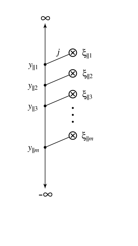
FIG. 2.: Diagrammatic representation of longitudinal structure of the $m$th-order term in the expression for the light-cone gauge vector potential, Eq. (60). The circled crosses denote the positions at which the sources are being evaluated. The dots represent the ordered integrations coning from the gauge transformation into the light-cone gauge.

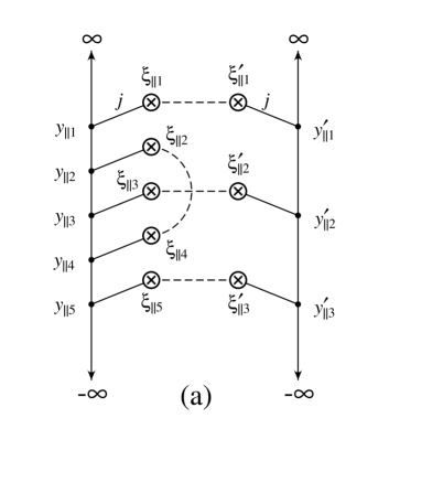
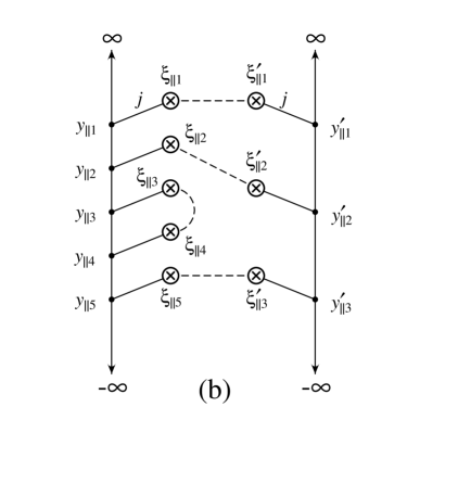
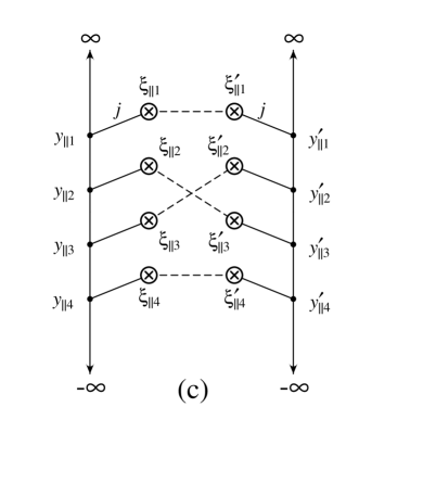
FIG. 3.: Some of the contributions to the gluon number density at 8th order in $\rho$. (a) Diagram containing a non-adjacent self-contraction. (b) Diagram containing an adjacent self-contraction. (c) Diagram containing a pair of crossed mutual contractions. (d) Diagram containing only corresponding mutual contractions. Diagrams (a) and (c) are suppressed by a power of $a/R$ relative to diagrams (b) and (d).

FIG. 4.: Plot of the nuclear correction function ${\cal E}(z)$ for negative values of $z$ and a spherical nucleus.

FIG. 5.: Position space correlation functions used to determine the fully differential gluon number density from Eq. (61) evaluated using the power-law model for $\widetilde{{\cal D}}(\vec{q}\thinspace)$ given in Eq. (71). The three curves compare the results using $\omega=1$, 2, and 8 at fixed $x_{{}_{F}}=0.1$ in the Abelian limit ($\alpha_{s}^{2}A^{1/3}=0$) and for uranium ($\alpha_{s}^{2}A^{1/3}=0.5$).

FIG. 6.: The fully differential gluon number density Eq. (61) evaluated in the power-law model with $\omega=1$. The three curves on each plot represent the Abelian limit ($\alpha_{s}^{2}A^{1/3}=0$), uranium ($\alpha_{s}^{2}A^{1/3}=0.5$), and a large toy nucleus with $A\sim 15000$ ($\alpha_{s}^{2}A^{1/3}=2.0$). The upper plot illustrates the results for $x_{{}_{F}}\rightarrow 0$, whereas the lower plot has been drawn for $x_{{}_{F}}=0.1$.

FIG. 7.: The fully differential gluon number density Eq. (61) multiplied by $\mathchoice{{\hbox{\boldmath$\displaystyle q$}}}{{\hbox{\boldmath$\textstyle q$}}}{{\hbox{\boldmath$\scriptstyle q$}}}{{\hbox{\boldmath$\scriptscriptstyle q$}}}^{2}$ and evaluated in the $\omega=1$ power-law model. These plots accurately reflect the relative contributions to the gluon structure function $g_{A}(x_{{}_{F}},Q^{2})$ coming from each value of $\mathchoice{{\hbox{\boldmath$\displaystyle q$}}}{{\hbox{\boldmath$\textstyle q$}}}{{\hbox{\boldmath$\scriptstyle q$}}}{{\hbox{\boldmath$\scriptscriptstyle q$}}}^{2}$. The three curves on each plot represent the Abelian limit ($\alpha_{s}^{2}A^{1/3}=0$), uranium ($\alpha_{s}^{2}A^{1/3}=0.5$), and a large toy nucleus with $A\sim 15000$ ($\alpha_{s}^{2}A^{1/3}=2.0$). The upper plot illustrates the results for $x_{{}_{F}}\rightarrow 0$, whereas the lower plot has been drawn for $x_{{}_{F}}=0.1$.

FIG. 8.: Value of the momentum-squared at the peak of the $\mathchoice{{\hbox{\boldmath$\displaystyle q$}}}{{\hbox{\boldmath$\textstyle q$}}}{{\hbox{\boldmath$\scriptstyle q$}}}{{\hbox{\boldmath$\scriptscriptstyle q$}}}^{2}dN/dx_{{}_{F}}d^{2}\mathchoice{{\hbox{\boldmath$\displaystyle q$}}}{{\hbox{\boldmath$\textstyle q$}}}{{\hbox{\boldmath$\scriptstyle q$}}}{{\hbox{\boldmath$\scriptscriptstyle q$}}}$ distribution as a function of the scale set by the non-Abelian corrections, $v^{2}\propto A^{1/3}\Lambda_{\rm QCD}^{2}$. These curves have been generated within the $\omega=1$ power-law model.

FIG. 9.: Gluon distribution function $g_{A}(x_{{}_{F}},Q^{2})$ in the $\omega=1$ power-law model plotted versus $x_{{}_{F}}$ for $Q^{2}=\Lambda_{\rm QCD}^{2}$, $10\Lambda_{\rm QCD}^{2}$, $100\Lambda_{\rm QCD}^{2}$, and $1000\Lambda_{\rm QCD}^{2}$. The three curves at each $Q^{2}$ value are for the Abelian limit ($\alpha_{s}^{2}A^{1/3}=0$), uranium ($\alpha_{s}^{2}A^{1/3}=0.5$), and a large toy nucleus with $A\sim 15000$ ($\alpha_{s}^{2}A^{1/3}=2.0$).

FIG. 10.: Nuclear dependence of the gluon distribution function $g_{A}(x_{{}_{F}},Q^{2})$ in the $\omega=1$ power-law model for fixed $x_{{}_{F}}=0.1$ and $Q^{2}=\Lambda_{\rm QCD}^{2}$, $2.5\Lambda_{\rm QCD}^{2}$, $10\Lambda_{\rm QCD}^{2}$, $25\Lambda_{\rm QCD}^{2}$, $100\Lambda_{\rm QCD}^{2}$, and $1000\Lambda_{\rm QCD}^{2}$. These functions grow more slowly than $A$ as the number of nucleons is increased.

FIG. 11.: Quark probability distributions as determined in the context of the Kovchegov model[13] for the power-law correlation function (71). The three curves compare the results for $\omega=1$, 2, and 8.