VUTH 00-20 Deep inelastic leptoproduction of spin-one hadrons

Abstract

In this paper we analyze deep inelastic one-particle inclusive processes for the case of spin-one targets or for the case of spin-one produced hadrons, such as $\rho$ mesons. This allows the measurement of new distribution and fragmentation functions not available in the spin-half case, and provides new ways to probe functions otherwise difficult to measure. We will analyze only contributions leading order in $1/Q$, but we will include effects of the transverse momentum of partons. We also include time-reversal odd functions.

I Introduction

Cross-sections in deep inelastic scattering (DIS) can be expressed in terms of distribution and fragmentation functions, which provide information on the quark and gluon structure of hadrons. The energy scale of the process is given by $Q^{2}=-q^{2}$, $q$ being the four-momentum transfer of the lepton. Depending on the number of observables one is able to measure, one can extract a variety of functions. The functions appearing in leading order in $1/Q$ can be interpreted as partonic probability densities.

We will study the case of one-particle inclusive experiments, which require measurement of one hadron among the ones produced in the scattering event. We will emphasize the importance of including transverse momenta of partons. We will also include T-odd functions. We will give a systematic list of the various functions that come into play up to leading order in $1/Q$ when we deal with either spin-1 targets or spin-1 outgoing hadrons. The second case is of interest to analyze vector meson production.

To properly study the distribution and fragmentation functions including transverse momentum dependence, we will start from a field-theoretical formalism, as outlined in [1]. This approach has been fully exploited only to study spin-$\frac{1}{2}$ targets and spin-$\frac{1}{2}$ outgoing hadrons. After an overview of the general properties of spin-1 particles and of the general formalism needed to deal with them (Sec. II), we turn to the most general parameterization of the correlation functions when spin-1 is included and we define the distribution and fragmentation functions (Sec. III). Distribution and fragmentation functions integrated over transverse momenta have been partially studied already in a number of papers [2, 3, 4]. An incomplete treatment of transverse momentum dependent functions has been performed in [5].

The distribution functions for a spin-1 target could be used for the deuteron, but is not the main goal of our study as the deuteron is in essence a weakly bound system of two spin-$\frac{1}{2}$ nucleons. The spin-1 distribution functions are useful as a passage to the fragmentation functions for spin-1 hadrons. The latter, however, require final state polarimetry of the produced hadron, i.e. the study of the angular distribution of its decay products. The most common of such hadrons is the $\rho$ meson. It is abundantly produced in leptoproduction experiments, e.g. at HERA, and it should be possible to measure its polarization in a detailed, as it has already been done in diffractive production [6, 7, 8] and in hadronic Z⁰ decay [9]. Another possibility is observation of polarization in inclusive leptoproduction of $\phi$ mesons, for which there should be less hadronic background.

In the last section we focus more specifically on deep-inelastic leptoproduction of spin-1 hadrons and we list all the possible cross-sections for different polarization conditions in terms of the usual spin-$\frac{1}{2}$ distribution functions and the newly defined spin-1 fragmentation functions.

II The description of spin-one particles

The description of particles with spin can be attained by using a spin density matrix $\rho$ in the rest-frame of the particle. The parameterization of the density matrix for a spin-J particle is conveniently performed with the introduction of irreducible spin tensors up to rank 2J. For example, the density matrix of a spin-$\frac{1}{2}$ particle can be decomposed on a Cartesian basis of $2\times 2$ matrices, formed by the identity matrix and the three Pauli matrices,

$${\mbox{\boldmath$\rho$}}=\frac{1}{2}\left({\mbox{\boldmath$1$}}+S^{i}{\mbox{\boldmath$\sigma$}}^{i}\right),$$ (1)

where we introduced the (rank-one) spin vector $S^{i}$.

To parameterize the density matrix of a spin-1 particle we can choose a Cartesian basis of $3\times 3$ matrices, formed by the identity matrix, three spin matrices ${\mbox{\boldmath$\Sigma$}}^{i}$ (generalization of the Pauli matrices to the three-dimensional case) and five extra matrices ${\mbox{\boldmath$\Sigma$}}^{ij}$. These last ones can be built using bilinear combinations of the spin matrices. In three dimensions these combinations are no more dependent on the spin matrices themselves, as it would be for the Pauli matrices. We choose them to be (see [10] and [11] for a comparison)

$${\mbox{\boldmath$\Sigma$}}^{ij}=\frac{1}{2}\left({\mbox{\boldmath$\Sigma$}}^{i}{\mbox{\boldmath$\Sigma$}}^{j}+{\mbox{\boldmath$\Sigma$}}^{j}{\mbox{\boldmath$\Sigma$}}^{i}\right)-\frac{2}{3}{\bf 1}\;\delta^{ij}.$$ (2)

With these preliminaries, we can write the spin density matrix as

$${\mbox{\boldmath$\rho$}}=\frac{1}{3}\left({\bf 1}+\frac{3}{2}S^{i}{\mbox{\boldmath$\Sigma$}}^{i}+3\,T^{ij}{\mbox{\boldmath$\Sigma$}}^{ij}\right),$$ (3)

where we introduced the symmetric traceless rank-two spin tensor $T^{ij}$.

We choose the following way of parameterizing the spin vector and tensor in the rest-frame of the hadron,

$$S = \left(S_{T}^{x},S_{T}^{y},S_{L}\right),$$ (4)

$$T = \frac{1}{2}\left(\begin{array}[]{ccc}-\frac{2}{3}{S_{LL}}+{S_{TT}^{xx}}&{S_{TT}^{xy}}&{S_{LT}^{x}}\\ {S_{TT}^{xy}}&-\frac{2}{3}{S_{LL}}-{S_{TT}^{xx}}&{S_{LT}^{y}}\\ {S_{LT}^{x}}&{S_{LT}^{y}}&\frac{4}{3}{S_{LL}}\\ \end{array}\right).$$ (9)

In App. A we give some explicit forms and other details of the density matrices and parameters involved in Eq. (9). In an arbitrary frame, different from the rest-frame, the spin vector and tensor satisfy the conditions $P_{\mu}S^{\mu}=0$ and $P_{\mu}T^{\mu\nu}=0$, where $P_{\mu}$ is the momentum of the hadron. In App. B we also discuss how the tensor polarization of a produced $\rho$-meson can be extracted from the angular distribution of the decay products $\pi^{+}\pi^{-}$.

III Correlation functions

Cross sections of DIS events are proportional to the contraction between a purely leptonic tensor and a purely hadronic tensor. While the leptonic tensor can be calculated theoretically, we are not able to do the same for the hadronic tensor, because we lack knowledge of the inner, non-perturbative structure of hadrons.

In the Bjorken limit, it is possible to separate the hadronic tensor into a hard part (virtual photon-quark scattering) and a soft part, containing the information on the parton distribution inside the hadron. This soft part is a correlation function, defined as the matrix element of quark fields between hadronic states. In one-particle inclusive processes we need two correlation functions, one describing the quark distributions in the target hadron and one describing the hadronization of a quark into the detected final state hadron.

In leading order in $1/Q$ (also referred to as “leading twist” or “twist-2”) we are concerned only with quark-quark correlation functions entering the handbag diagram in Fig. 1. They are defined as follows (using Dirac indices $\alpha$ and $\beta$):

$$\Phi_{\alpha\beta}(p,P,S,T) = \int\frac{{\rm\,d}^{4}\xi}{(2\pi)^{4}}{\rm e}^{-{\rm i}p\cdot\xi}\langle P,S,T|\overline{\psi}_{\beta}(\xi)\psi_{\alpha}(0)|P,S,T\rangle,$$ (10)

$$\Delta_{\alpha\beta}(k,P_{h},S_{h},T_{h}) = \int\frac{{\rm\,d}^{4}\xi}{(2\pi)^{4}}{\rm e}^{+{\rm i}k\cdot\xi}\langle 0|\psi_{\alpha}(\xi)|P_{h},S_{h},T_{h}\rangle\langle P_{h},S_{h},T_{h}|\overline{\psi}_{\beta}(0)|0\rangle,$$ (11)

and describe the quark distribution and fragmentation, respectively. Here, $p$ is the momentum of the quark emerging from the target, while $k$ is the momentum of the quark decaying into an outgoing hadron after being struck by a virtual photon (see Fig. 1). The vector $P$ ($P_{h}$) is the momentum of the hadronic target (outgoing hadron), the quantities $S$ ($S_{h}$) and $T$ ($T_{h}$) are the spin vector and tensor.

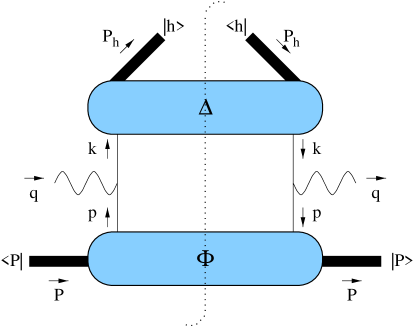
FIG. 1.: Diagrammatic representation of semi-inclusive DIS

The correlation functions can be expressed in several terms, each one being a combination of the Lorentz vectors $p$ ($k$) and $P$ ($P_{h}$), the Lorentz pseudo-vector $S$ ($S_{h}$), the Lorentz tensor $T$ ($T_{h}$) and the Dirac structures

$\displaystyle 1\rule[0.34444pt]{0.45pt}{6.45831pt}\hskip 2.0pt,\;\gamma_{5},\;\gamma^{\mu},\;\gamma^{\mu}\gamma_{5},\;{\rm i}\sigma^{\mu\nu}\gamma_{5}.$The spin vector and tensor can only appear linearly in the decomposition. Moreover, each term of the full expression has to fulfill the conditions of hermiticity and parity invariance

$$\Phi(p,P,S,T) = \gamma^{0}\Phi^{{\dagger}}(p,P,S,T)\gamma^{0}$$ hermiticity, (12)

$$\Phi(p,P,S,T) = \gamma^{0}\Phi(\tilde{p},\tilde{P},-\tilde{S},\tilde{T})\gamma^{0}$$ parity, (13)

where $\tilde{p}$, $\tilde{P}$ and $\tilde{S}$ represent respectively the vectors $p$, $P$ and $S$ having space components with inverted sign and $\tilde{T}$ represents the tensor $T$ having mixed space-time components with inverted sign. For the distribution part $\Phi$ one also obtains a constraint from time-reversal inversion (leaving out effective T-odd parts coming from for instance gluonic poles [12, 13])

$$\Phi(p,P,S,T) = \makebox[142.26378pt][l]{$\gamma^{1}\gamma^{3}\,\Phi^{*}(\tilde{p},\tilde{P},\tilde{S},\tilde{T})\,\gamma^{3}\gamma^{1}$}\mbox{time-reversal}.$$ (14)

For the fragmentation part $\Delta$, containing out-states in the definition, time-reversal invariance cannot be used as a constraint [14, 15, 16] and one is left with the so-called time-reversal odd (T-odd) contributions, leading in particular to interesting single spin asymmetries [17, 18]. We will include the T-odd contributions in our discussion for $\Phi$, because it will be used as the general case of correlation functions. Throughout the rest of the article we will put time-reversal odd terms between brackets to make them easily identifiable.

The most general decompositions of the correlation function $\Phi$ imposing hermiticity and parity is

$$\Phi(p,P,S,T) = M\,A_{1}\,1\rule[0.34444pt]{0.45pt}{6.45831pt}\hskip 2.0pt+A_{2}\,\kern 1.99997ptP\kern-5.59998pt\raisebox{1.29167pt}{/}+A_{3}\kern 1.99997ptp\kern-3.99994pt/+\left(\frac{A_{4}}{M}\,\sigma_{\mu\nu}P^{\mu}p^{\nu}\right)+\left({\rm i}A_{5}\;p\cdot S\,\gamma_{5}\right)$$ (20)

$$\mbox{}+M\,A_{6}\,\kern 1.99997ptS\kern-5.59998pt\raisebox{1.29167pt}{/}\,\gamma_{5}+A_{7}\,\frac{p\cdot S}{M}\,\kern 1.99997ptP\kern-5.59998pt\raisebox{1.29167pt}{/}\,\gamma_{5}+A_{8}\,\frac{p\cdot S}{M}\kern 1.99997ptp\kern-3.99994pt/\,\gamma_{5}+{\rm i}A_{9}\,\sigma_{\mu\nu}\gamma_{5}S^{\mu}P^{\nu}$$

$$\mbox{}+{\rm i}A_{10}\,\sigma_{\mu\nu}\gamma_{5}S^{\mu}p^{\nu}+{\rm i}A_{11}\,\frac{p\cdot S}{M^{2}}\,\sigma_{\mu\nu}\gamma_{5}P^{\mu}p^{\nu}+\left(A_{12}\,\frac{\epsilon_{\mu\nu\rho\sigma}\gamma^{\mu}P^{\nu}p^{\rho}S^{\sigma}}{M}\right)$$

$$\mbox{}+\frac{A_{13}}{M}\,p_{\mu}p_{\nu}T^{\mu\nu}\,1\rule[0.34444pt]{0.45pt}{6.45831pt}\hskip 2.0pt+\frac{A_{14}}{M^{2}}\;p_{\mu}p_{\nu}T^{\mu\nu}\kern 1.99997ptP\kern-5.59998pt\raisebox{1.29167pt}{/}+\frac{A_{15}}{M^{2}}\;p_{\mu}p_{\nu}T^{\mu\nu}\kern 1.99997ptp\kern-3.99994pt/$$

$$\mbox{}+\left(\frac{A_{16}}{M^{3}}\;p_{\mu}p_{\nu}T^{\mu\nu}\sigma_{\rho\sigma}P^{\rho}p^{\sigma}\right)+A_{17}\;p_{\mu}T^{\mu\nu}\gamma_{\nu}+\left(\frac{A_{18}}{M}\,\sigma_{\nu\rho}P^{\rho}\,p_{\mu}T^{\mu\nu}\right)$$

$$\mbox{}+\left(\frac{A_{19}}{M}\,\sigma_{\nu\rho}p^{\rho}\,p_{\mu}T^{\mu\nu}\right)+\left(\frac{A_{20}}{M^{2}}\,\epsilon_{\mu\nu\rho\sigma}\gamma^{\mu}\gamma_{5}P^{\nu}p^{\rho}\,p_{\tau}T^{\tau\sigma}\right).$$

The amplitudes $A_{i}$ are real functions $A_{i}=A_{i}(p\cdot P,p^{2})$. The decomposition of the correlation function $\Delta$ is analogous. The amplitudes $A_{4}$, $A_{5}$, $A_{12}$, $A_{16}$, $A_{18}$, $A_{19}$ and $A_{20}$ are T-odd.

In order to select leading twist contributions we perform a Sudakov decomposition of the Lorentz structures we have. We choose two light-like vectors $n_{+}$ and $n_{-}$ satisfying $n_{+}\cdot n_{-}=1$. We will call the plane perpendicular to these vectors “transverse plane”. We define the two projectors

$$g_{T}^{\mu\nu} = g^{\mu\nu}-n_{+}^{\{\mu}n_{-}^{\nu\}},$$ (21)

$$\epsilon_{T}^{\mu\nu} = \epsilon^{\mu\nu\rho\sigma}n_{+\,\rho}n_{-\,\sigma},$$ (22)

where the curly braces around the indices denote symmetrization of these indices. Given a vector $a^{\mu}$ we will sometimes make use of the notation $a_{T}^{\mu}=g_{T}^{\mu\nu}a_{\nu}$ and we will denote its two-dimensional component lying in the transverse plane as ${\mbox{\boldmath$a$}}_{T}$.

We assume the following decompositions of the Lorentz structures we are interested in:

$$P^{\mu} = P^{+}n_{+}^{\mu}+\frac{M^{2}}{2P^{+}}n_{-}^{\mu},$$ (23)

$$p^{\mu} = xP^{+}n_{+}^{\mu}+p_{T}^{\mu}+p^{-}n_{-}^{\mu},\phantom{\frac{M}{P}}$$ (24)

$$S^{\mu} = S_{L}\,\frac{P^{+}}{M}n_{+}^{\mu}+S_{T}^{\mu}-S_{L}\,\frac{M}{2P^{+}}n_{-}^{\mu},$$ (25)

$$T^{\mu\nu} = \frac{1}{2}\Biggl{[}\frac{4}{3}\,S_{LL}\,\frac{{(P^{+})}^{2}}{M^{2}}\,n_{+}^{\mu}n_{+}^{\nu}+\frac{P^{+}}{M}\,n_{+}^{\{\mu}S_{LT}^{\nu\}}$$ (28)

$$\qquad\mbox{}-\frac{2}{3}\,S_{LL}\,\left(n_{+}^{\{\mu}n_{-}^{\nu\}}-g_{T}^{\mu\nu}\right)+{S_{TT}^{\mu\nu}}$$

$$\qquad\mbox{}-\frac{M}{2P^{+}}\,n_{-}^{\{\mu}{S_{LT}^{\nu\}}}+\frac{1}{3}\,S_{LL}\,\frac{M^{2}}{{(P^{+})}^{2}}\,n_{-}^{\mu}n_{-}^{\nu}\Biggr{]}$$

When only one hadron is considered, e.g. in inclusive DIS, there is an arbitrariness in the choice of $n_{-}$, though this does not affect physical observables. In processes where another hadron is present, such as one-particle inclusive leptoproduction, $n_{-}$ can be conveniently connected to the momentum of the produced hadron, so that $P^{\mu}=P_{h}^{-}n_{-}^{\mu}+(M_{h}^{2}/2P_{h}^{-})n_{+}^{\mu}$ . This choice of light-like directions is particularly useful to analyze current fragmentation in leptoproduction. In this case one finds that up to order in $1/Q^{2}$ only one light-like component of the hadron momentum is relevant. If we choose the relevant component of the target momentum to be $P^{+}$, then the relevant component of the outgoing hadron momentum will be $P_{h}^{-}$. We need to define the decomposition of the fragmenting quark momentum $k^{\mu}=(1/z)P_{h}^{-}n_{-}^{\mu}+k_{T}^{\mu}+k^{+}n_{-}^{\mu}$, while to obtain the decomposition for the outgoing hadron’s spin vector and tensor, it is sufficient to interchange the $+$ and $-$ components in Eq. (25) and Eq. (28).

In semi-inclusive DIS one needs to consider the following integrated correlation function:

$$\Phi(x,{\mbox{\boldmath$p$}}_{T}) = \frac{1}{2}\left.\int{\rm\,d}p^{-}\;\Phi(p,P,S,T)\right|_{p^{+}=xP^{+}}\,,$$ (29)

$$\Delta(z,{\mbox{\boldmath$k$}}_{T}) = \frac{1}{4z}\left.\int{\rm\,d}k^{+}\;\Delta(k,P_{h},S_{h},T_{h})\right|_{k^{-}=\frac{P_{h}^{-}}{z}}\,.$$ (30)

In inclusive processes or after integrating the semi-inclusive cross sections over the outgoing hadron’s perpendicular momentum one needs to consider the following ones:

$$\Phi(x) = \frac{1}{2}\left.\int{\rm\,d}^{2}{\mbox{\boldmath$p$}}_{T}\,{\rm\,d}p^{-}\;\Phi(k,P_{h},S_{h},T_{h})\right|_{p^{+}=xP^{+}}\,,$$ (31)

$$\Delta(z) = \frac{z}{4}\left.\int{\rm\,d}^{2}{\mbox{\boldmath$k$}}_{T}\,{\rm\,d}k^{+}\;\Delta(k,P_{h},S_{h},T_{h})\right|_{k^{-}=\frac{P_{h}^{-}}{z}}.$$ (32)

Note that in the case of fragmentation, it is conventional to integrate over $-z\,\mbox{\boldmath$k$}_{T}$, which is the transverse momentum of the produced hadron with respect to the quark. This can be checked by applying a Lorentz transformation that does not affect the minus component nor the integration over the plus component. Using coordinates $[a^{-},a^{+},\mbox{\boldmath$a$}_{T}]$, the required transformation is

$$\left[P_{h}^{-},\frac{M_{h}^{2}}{2P_{h}^{-}},\mbox{\boldmath$0$}_{T}\right] \quad\rightarrow\quad \left[P_{h}^{-},\frac{M^{2}+z^{2}\,\mbox{\boldmath$k$}_{T}^{2}}{2P_{h}^{-}},-z\,\mbox{\boldmath$k$}_{T}\right]$$ (33)

$$\left[\frac{P_{h}^{-}}{z},k^{+},\mbox{\boldmath$k$}_{T}\right] \quad\rightarrow\quad \left[\frac{P_{h}^{-}}{z},k^{+}-\frac{z\,\mbox{\boldmath$k$}_{T}^{2}}{2P_{h}^{-}},\mbox{\boldmath$0$}_{T}\right].$$ (34)

We are going to separate different parts of the correlation functions depending on the polarization conditions they require to be observed. We will use the subscript $U$ to denote unpolarized hadrons, the subscript $L$ and $T$ to denote respectively longitudinal and transverse vector polarization and finally the subscripts $LL$, $LT$ and $TT$ to denote longitudinal-longitudinal, longitudinal-transverse and transverse-transverse tensor polarization.

In leading order in $1/Q$, the parameterization of the ${\mbox{\boldmath$p$}}_{T}$ dependent correlation function, defined in Eq. (29), is (we remind the reader that terms in round brackets are T-odd)

$$\Phi_{U}(x,{\mbox{\boldmath$p$}}_{T}) = \frac{1}{4}\left\{f_{1}(x,p_{T}^{2})\,\kern 1.99997ptn\kern-5.0pt/_{+}+\left(h_{1}^{\perp}(x,p_{T}^{2})\,\sigma_{\mu\nu}\frac{p_{T}^{\mu}}{M}n_{+}^{\nu}\right)\right\},$$ (35)

$$\Phi_{L}(x,{\mbox{\boldmath$p$}}_{T}) = \frac{1}{4}\left\{g_{1L}(x,p_{T}^{2})\,S_{L}\,\gamma_{5}\kern 1.99997ptn\kern-5.0pt/_{+}+h_{1L}^{\perp}(x,p_{T}^{2})\,S_{L}\,{\rm i}\sigma_{\mu\nu}\gamma_{5}n_{+}^{\mu}\frac{p_{T}^{\nu}}{M}\right\},$$ (36)

$$\Phi_{T}(x,{\mbox{\boldmath$p$}}_{T}) = \frac{1}{4}\left\{g_{1T}(x,p_{T}^{2})\,\frac{{\mbox{\boldmath$S$}}_{T}\cdot{\mbox{\boldmath$p$}}_{T}}{M}\,\gamma_{5}\kern 1.99997ptn\kern-5.0pt/_{+}+h_{1T}(x,p_{T}^{2})\,{\rm i}\sigma_{\mu\nu}\gamma_{5}n_{+}^{\mu}S_{T}^{\nu}\right.$$ (39)

$$\left.\mbox{}+h_{1T}^{\perp}(x,p_{T}^{2})\,\frac{{\mbox{\boldmath$S$}}_{T}\cdot{\mbox{\boldmath$p$}}_{T}}{M}\,{\rm i}\sigma_{\mu\nu}\gamma_{5}n_{+}^{\mu}\frac{p_{T}^{\nu}}{M}\right.$$

$$\left.\mbox{}+\left(f^{\perp}_{1T}(x,p_{T}^{2})\,\epsilon_{\mu\nu\rho\sigma}\gamma^{\mu}n_{+}^{\nu}\frac{p_{T}^{\rho}}{M}S_{T}^{\sigma}\right)\right\},$$

$$\Phi_{LL}(x,{\mbox{\boldmath$p$}}_{T}) = \frac{1}{4}\left\{f_{1LL}(x,p_{T}^{2})\,S_{LL}\,\kern 1.99997ptn\kern-5.0pt/_{+}+\left(h_{1LL}^{\perp}(x,p_{T}^{2})\,S_{LL}\,\sigma_{\mu\nu}\frac{p_{T}^{\mu}}{M}n_{+}^{\nu}\right)\right\},$$ (40)

$$\Phi_{LT}(x,{\mbox{\boldmath$p$}}_{T}) = \frac{1}{4}\left\{f_{1LT}(x,p_{T}^{2})\,\frac{{\mbox{\boldmath$S$}}_{LT}\cdot{\mbox{\boldmath$p$}}_{T}}{M}\,\kern 1.99997ptn\kern-5.0pt/_{+}+\left(g_{1LT}(x,p_{T}^{2})\,\epsilon_{T}^{\mu\nu}S_{LT\,\mu}\frac{p_{T\,\nu}}{M}\,\gamma_{5}\kern 1.99997ptn\kern-5.0pt/_{+}\right)\right.$$ (43)

$$\left.\mbox{}+\left(h^{\prime}_{1LT}(x,p_{T}^{2})\,{\rm i}\sigma_{\mu\nu}\gamma_{5}n_{+}^{\mu}\epsilon_{T}^{\nu\rho}S_{LT\,\rho}\right)\right.$$

$$\left.\mbox{}+\left(\,h_{1LT}^{\perp}(x,p_{T}^{2})\,\frac{{\mbox{\boldmath$S$}}_{LT}\cdot{\mbox{\boldmath$p$}}_{T}}{M}\,\sigma_{\mu\nu}\frac{p_{T}^{\mu}}{M}n_{+}^{\nu}\right)\right\},$$

$$\Phi_{TT}(x,{\mbox{\boldmath$p$}}_{T}) = \frac{1}{4}\left\{f_{1TT}(x,p_{T}^{2})\,\frac{{\mbox{\boldmath$p$}}_{T}\cdot{\mbox{\boldmath$S$}}_{TT}\cdot{\mbox{\boldmath$p$}}_{T}}{M^{2}}\,\kern 1.99997ptn\kern-5.0pt/_{+}\right.$$ (47)

$$\left.\mbox{}-\left(g_{1TT}(x,p_{T}^{2})\,\epsilon_{T}^{\mu\nu}S_{TT\,\nu\rho}\frac{p_{T}^{\rho}p_{T\,\mu}}{M^{2}}\,\gamma_{5}\kern 1.99997ptn\kern-5.0pt/_{+}\right)\right.$$

$$\left.\mbox{}-\left(h^{\prime}_{1TT}(x,p_{T}^{2})\,{\rm i}\sigma_{\mu\nu}\gamma_{5}n_{+}^{\mu}\epsilon_{T}^{\nu\rho}S_{TT\,\rho\sigma}\frac{p_{T}^{\sigma}}{M}\right)\right.$$

$$\left.\mbox{}+\left(\,h_{1TT}^{\perp}(x,p_{T}^{2})\,\frac{{\mbox{\boldmath$p$}}_{T}\cdot{\mbox{\boldmath$S$}}_{TT}\cdot{\mbox{\boldmath$p$}}_{T}}{M^{2}}\,\sigma_{\mu\nu}\frac{p_{T}^{\mu}}{M}n_{+}^{\nu}\right)\right\}.$$

The parameterization of the correlation function after integration upon ${\mbox{\boldmath$p$}}_{T}$, as defined in Eq. (31), is

$$\Phi_{U}(x) = \frac{1}{4}\,f_{1}(x)\kern 1.99997ptn\kern-5.0pt/_{+},$$ (48)

$$\Phi_{L}(x) = \frac{1}{4}\,g_{1}(x)\,S_{L}\,\gamma_{5}\kern 1.99997ptn\kern-5.0pt/_{+},$$ (49)

$$\Phi_{T}(x) = \frac{1}{4}\,h_{1}(x)\,{\rm i}\sigma_{\mu\nu}\gamma_{5}n_{+}^{\mu}S_{T}^{\nu},$$ (50)

$$\Phi_{LL}(x) = \frac{1}{4}f_{1LL}(x)\,S_{LL}\,\kern 1.99997ptn\kern-5.0pt/_{+},$$ (51)

$$\Phi_{LT}(x) = \frac{1}{4}\,\left(h_{1LT}(x)\,{\rm i}\sigma_{\mu\nu}\gamma_{5}n_{+}^{\mu}\epsilon_{T}^{\nu\rho}S_{LT\,\rho}\right),$$ (52)

$$\Phi_{TT}(x) = 0,$$ (53)

where

$$g_{1}(x) = \int{\rm\,d}^{2}{\mbox{\boldmath$p$}}_{T}\;g_{1L}(x,{p}^{2}_{T}),$$ (54)

$$h_{1}(x) = \int{\rm\,d}^{2}{\mbox{\boldmath$p$}}_{T}\;h_{1}(x,{p}^{2}_{T})\;=\;\int{\rm\,d}^{2}{\mbox{\boldmath$p$}}_{T}\left(h_{1T}(x,{p}^{2}_{T})+\frac{{\mbox{\boldmath$p$}}_{T}^{2}}{2M^{2}}\;h_{1T}^{\perp}(x,{p}^{2}_{T})\right),$$ (55)

$$h_{1LT}(x) = \int{\rm\,d}^{2}{\mbox{\boldmath$p$}}_{T}\;h_{1LT}(x,{p}^{2}_{T})\;=\;\int{\rm\,d}^{2}{\mbox{\boldmath$p$}}_{T}\left(h^{\prime}_{1LT}(x,{p}^{2}_{T})+\frac{{\mbox{\boldmath$p$}}_{T}^{2}}{2M^{2}}\;h_{1LT}^{\perp}(x,{p}^{2}_{T})\right).$$ (56)

The decomposition of the correlation function $\Delta$ is identical after the replacements $\{x,p_{T},S,M,n_{+}\}\rightarrow\{z,k_{T},S_{h},M_{h},n_{-}\}$ and the notation replacement $f\rightarrow D$, $g\rightarrow G$, $h\rightarrow H$.

In App. C all the possible distribution functions are projected out of the complete correlation function. In Tab. I and Tab. II we give a summary of all the distribution functions, respectively before and after integration upon ${\mbox{\boldmath$p$}}_{T}$.

The function $f_{1LL}$ has been already studied in [2], where it was given the name $b_{1}$ (Note that actually $f_{1LL}$ = $-\frac{2}{3}\,b_{1}$). Although this name has been already used also by other authors (e.g. [5, 4]), we felt the need to change it to follow a more systematic naming. The function $f_{1LT}$ is analogous to the function $c_{1}$ introduced in [5], although the different approach followed in that article requires a more careful comparison.

It is worthwhile to note that, as suggested by Eq. (52), dealing with spin-1 particles offers the possibility of measuring a time-reversal odd function in leading twist and without considering intrinsic transverse momentum. The particular fragmentation function $H_{1LT}$, equivalent to the distribution function $h_{1LT}$, has been introduced in [3], where it was named $\hat{h}_{\bar{1}}$.

	$[\gamma^{+}]$		$[\gamma^{+}\gamma_{5}]$		$[{\rm i}\sigma^{i+}\gamma_{5}]$
	TR-even	TR-odd	TR-even	TR-odd	TR-even	TR-odd
U	$f_{1}$					$(h_{1}^{\perp})$
L			$g_{1L}$		$h_{1L}^{\perp}$
T		$(f_{1T}^{\perp})$	$g_{1T}$		$h_{1T}$ $h_{1T}^{\perp}$
LL	$f_{1LL}$					$(h_{1LL}^{\perp})$
LT	$f_{1LT}$			$(g_{1LT})$		$(h^{\prime}_{1LT}$ $h_{1LT}^{\perp})$
TT	$f_{1TT}$			$(g_{1TT})$		$(h^{\prime}_{1TT}$ $h_{1TT}^{\perp})$

TABLE I.: List of leading twist distribution functions, divided in time-reversal even and time-reversal odd

	$[\gamma^{+}]$		$[\gamma^{+}\gamma_{5}]$		$[{\rm i}\sigma^{i+}\gamma_{5}]$
	TR-even	TR-odd	TR-even	TR-odd	TR-even	TR-odd
U	$f_{1}$
L			$g_{1}$
T					$h_{1}$
LL	$f_{1LL}$
LT						$(h_{1LT})$
TT

TABLE II.: List of remaining leading twist distribution functions after integration upon ${\mbox{\boldmath$p$}}_{T}$, divided in time-reversal even and time-reversal odd

It is sometimes useful (for instance for calculation of azimuthal asymmetries) to consider the $p_{T}^{\alpha}$-weighted function

$$\frac{1}{M}\Phi_{\partial}^{\alpha}(x)\equiv\int{\rm\,d}^{2}{\mbox{\boldmath$p$}}_{T}\,\frac{p_{T}^{\alpha}}{M}\,\Phi(x,{\mbox{\boldmath$p$}}_{T}).$$ (57)

Non vanishing at twist two we have

$$\frac{1}{M}\left(\Phi_{\partial}^{\alpha}\right)_{U}(x) = -\frac{1}{4}\left(h_{1}^{\perp(1)}(x)\,\sigma^{\alpha\nu}n_{+\,\nu}\right),$$ (58)

$$\frac{1}{M}\left(\Phi_{\partial}^{\alpha}\right)_{L}(x) = -\frac{1}{4}\;h_{1L}^{\perp(1)}(x)\,S_{L}\,{\rm i}\sigma^{\mu\alpha}\gamma_{5}n_{+\,\mu},$$ (59)

$$\frac{1}{M}\left(\Phi_{\partial}^{\alpha}\right)_{T}(x) = -\frac{1}{4}\left\{g_{1T}^{(1)}(x)\,S_{T}^{\alpha}\,\gamma_{5}\kern 1.99997ptn\kern-5.0pt/_{+}+\left(f^{\perp(1)}_{1T}(x)\,\epsilon^{\mu\nu\alpha\sigma}\gamma_{\mu}n_{+\,\nu}S_{T\,\sigma}\right)\right\},$$ (60)

$$\frac{1}{M}\left(\Phi_{\partial}^{\alpha}\right)_{LL}(x) = -\frac{1}{4}\left(h_{1LL}^{\perp(1)}(x)\,S_{LL}\,\sigma^{\alpha\nu}n_{+\,\nu}\right),$$ (61)

$$\frac{1}{M}\left(\Phi_{\partial}^{\alpha}\right)_{LT}(x) = -\frac{1}{4}\left\{f_{1LT}^{(1)}(x)\,S_{LT}^{\alpha}\,\kern 1.99997ptn\kern-5.0pt/_{+}+\left(g_{1LT}^{(1)}(x)\,\epsilon_{T}^{\mu\alpha}S_{LT\,\mu}\,\gamma_{5}\kern 1.99997ptn\kern-5.0pt/_{+}\right)\right\},$$ (62)

$$\frac{1}{M}\left(\Phi_{\partial}^{\alpha}\right)_{TT}(x) = \frac{1}{4}\left(h_{1TT}^{(1)}(x)\,S_{TT}^{\alpha\mu}\,\sigma_{\mu\nu}n_{+}^{\nu}\right),$$ (63)

where we used the notation

$$h_{1}^{\perp(1)}(x)=\int{\rm\,d}^{2}{\mbox{\boldmath$p$}}_{T}\;h_{1}^{\perp(1)}(x,{p}^{2}_{T})=\int{\rm\,d}^{2}{\mbox{\boldmath$p$}}_{T}\,\frac{{\mbox{\boldmath$p$}}_{T}^{2}}{2M^{2}}\;h_{1}^{\perp}(x,{p}^{2}_{T}),$$ (64)

and we introduced the function

$$h_{1TT}(x,{p}^{2}_{T})=h^{\prime}_{1TT}(x,{p}^{2}_{T})+\frac{{\mbox{\boldmath$p$}}_{T}^{2}}{2M^{2}}\;h_{1TT}^{\perp}(x,{p}^{2}_{T}).$$ (65)

IV Semi-inclusive cross sections with tensor polarization in the final state

We consider one-particle inclusive DIS events where the target consists of a spin-$\frac{1}{2}$ hadron and the fragment is a spin-1 hadron with tensor polarization only. We allow only time-reversal odd fragmentation functions to occur, assuming that there are no time-reversal odd distribution function.

A short note on the kinematics is the first necessary ingredient. In Sec. III we defined with the help of the momenta $P$ and $P_{h}$ the transverse projector $g_{T}^{\mu\nu}$ and transverse vectors. From the experimental point of view it is customary to work with vectors constructed from the momenta $q$ and $P$. They are used to define a space-like direction $\hat{q}^{\mu}=q^{\mu}/Q$, an orthogonal time-like direction $\hat{t}^{\mu}=\frac{1}{Q}(2{x_{\scriptscriptstyle B}}P^{\mu}+q^{\mu})$, where $x_{\scriptscriptstyle B}=Q^{2}/2(P\cdot q)$ (neglecting mass corrections of order $1/Q^{2}$), and perpendicular directions via the tensor

$$g_{\perp}^{\mu\nu}=g^{\mu\nu}+\hat{q}^{\mu}\hat{q}^{\nu}-\hat{t}^{\mu}\hat{t}^{\nu}.$$ (66)

After introducing the scaling variable $z_{h}=2P_{h}\cdot q/Q^{2}\simeq P\cdot P_{h}/P\cdot q$ (neglecting order $1/Q^{2}$ corrections) and using $g_{T}^{\mu\nu}$ or $g_{\perp}^{\mu\nu}$ we can write the relation

$$x_{\scriptscriptstyle B}P^{\mu}-\frac{P_{h}^{\mu}}{z_{h}}+q^{\mu}=q_{T}^{\mu}=-\frac{P_{h\perp}^{\mu}}{z_{h}},$$ (67)

showing that the combination on the left-hand side is either the transverse component of $q$ (since $P_{T}=P_{hT}$ = 0) or the perpendicular component of $-P_{h}/z_{h}$ (since $P_{\perp}=q_{\perp}$ = 0).

To explicitly write cross sections we also need the scaling variable $y={P\cdot q}/{P\cdot l}$, where $l$ denotes the incoming lepton momentum, and the azimuthal angle $\phi^{\ell}$ of the lepton scattering plane. Cross sections will be differential with respect to the variables $x_{\scriptscriptstyle B}$, $z_{h}$, $y$, $\phi^{\ell}$ and ${\mbox{\boldmath$P$}}_{h\perp}$. When they do not vanish, we will also give cross sections integrated over ${\mbox{\boldmath$P$}}_{h\perp}$ and $\phi^{\ell}$. The general formula is

$$\frac{2\pi\,{\rm\,d}\sigma(l+H\rightarrow l^{\prime}+h+X)}{{\rm\,d}\phi^{\ell}{\rm\,d}x_{\scriptscriptstyle B}{\rm\,d}z_{h}{\rm\,d}y{\rm\,d}^{2}{\mbox{\boldmath$P$}}_{h\perp}}=\frac{\pi\alpha^{2}}{2Q^{4}}\;\frac{y}{z_{h}}\;L_{\mu\nu}\;2MW^{\mu\nu},$$ (68)

where $L_{\mu\nu}$ is the lepton tensor and $W^{\mu\nu}$ is the hadronic tensor given by the convolution of the soft parts,

$$2MW^{\mu\nu} = 2z_{h}\int{\rm\,d}^{2}{\mbox{\boldmath$p$}}_{T}{\rm\,d}^{2}{\mbox{\boldmath$k$}}_{T}\ \delta^{2}({\mbox{\boldmath$p$}}_{T}+{\mbox{\boldmath$q$}}_{T}-{\mbox{\boldmath$k$}}_{T})\;\mbox{Tr}\,\left[2\Phi(x_{\scriptscriptstyle B},{\mbox{\boldmath$p$}}_{T})\,\gamma^{\mu}\;2\Delta(z_{h},{\mbox{\boldmath$k$}}_{T})\,\gamma^{\nu}\right],$$ (69)

where it is understood that a summation over the charge squared weighted sum over quark flavors has to be included. The full form of the hadronic tensor can be obtained by introducing the correlation functions described in the previous section (see App. D). To shorten the formulae we will use the notation

$${\mbox{\boldmath$I$}}\left[\ldots\right]=2z_{h}\int{\rm\,d}^{2}{\mbox{\boldmath$p$}}_{T}{\rm\,d}^{2}{\mbox{\boldmath$k$}}_{T}\,\delta^{2}({\mbox{\boldmath$p$}}_{T}+{\mbox{\boldmath$q$}}_{T}-{\mbox{\boldmath$k$}}_{T})\ldots.$$ (70)

It is convenient to express the perpendicular vectors with respect to the only measured perpendicular direction, i.e. that of ${\mbox{\boldmath$P$}}_{h\perp}$, the outgoing hadron’s perpendicular momentum. Defining the unit vector in this direction $\hat{\mbox{\boldmath$h$}}=\frac{{\mbox{\boldmath$P$}}_{h\perp}}{|P_{h\perp}|}$, we are then going to use the following notation

$$a_{\perp}^{\mu} = a_{x}\,\hat{h}^{\mu}+a_{y}\,\epsilon_{\perp}^{\mu\nu}\hat{h}_{\nu}.$$ (71)

As it has been shown in [1], the difference between $g_{T}^{\mu\nu}$ in Eq. (21) and $g_{\perp}^{\mu\nu}$ in Eq. (66) is of order 1/Q, i.e. (neglecting order $1/Q^{2}$ parts)

$$g_{\perp}^{\mu\nu}=g_{T}^{\mu\nu}-\frac{\sqrt{2}n_{+}^{\{\mu}q_{T}^{\nu\}}}{Q}\qquad\mbox{or}\qquad g_{T}^{\mu\nu}=g_{\perp}^{\mu\nu}-\frac{Q_{T}}{Q}\sqrt{2}n_{+}^{\{\mu}\hat{h}^{\nu\}},$$ (72)

where $Q_{T}=|P_{h\perp}|/z_{h}$. This relation implies that if we already have projected out a transverse vector, the additional projection with $g_{\perp}^{\mu\nu}$ does not give additional terms, i.e. $a_{T\perp}^{\mu}$ = $g_{\perp}^{\mu\rho}a_{T\rho}=a_{T}^{\mu}$, even if $a_{\perp}^{\mu}\not=a_{T}^{\mu}$ (see App. B). This is true up to corrections of order $1/Q^{2}$.

We will indicate as $\phi_{S}^{h}$ the angle between ${\mbox{\boldmath$S$}}_{T}$ and ${\mbox{\boldmath$P$}}_{h\perp}$, as $\phi_{h}^{\ell}$ the angle between ${\mbox{\boldmath$P$}}_{h\perp}$ and the scattering plane, as $\phi_{S}^{\ell}$ the angle between ${\mbox{\boldmath$S$}}_{T}$ and the scattering plane.

For the tensor $T_{h}$ we introduce azimuthal angles defined as:

$$\tan{(\phi_{h\,LT}^{h})} = \;\tan{(\phi_{h\,LT}^{\ell}-\phi_{h}^{\ell})}\;=\;\frac{S_{h\,LT}^{y}}{S_{h\,LT}^{x}}\;,$$ (73)

$$\tan{(2\phi_{h\,TT}^{h})} = \tan{(2\phi_{h\,TT}^{\ell}-2\phi_{h}^{\ell})}\;=\;\frac{S_{h\,TT}^{xy}}{S_{h\,TT}^{xx}}\;,$$ (74)

and the the quantities

$$|S_{h\,LT}|\;=\;\sqrt{(S_{h\,LT}^{x})^{2}+(S_{h\,LT}^{y})^{2}}\;,\qquad|S_{h\,TT}|\;=\;\sqrt{(S_{h\,TT}^{xx})^{2}+(S_{h\,TT}^{xy})^{2}}\;.$$ (75)

In a real experiment, where polarimetry is performed on the final-state hadron, cross section will not depend on the spin tensor parameters but rather on the analyzing powers determined from the momenta of decay products. We omit writing explicit differential cross sections in terms of the momenta of the decay products, but we merely point out that spin tensor parameters in cross section formulae must be replaced by the corresponding analyzing powers, as given in App. B.

A Unpolarized lepton beam and unpolarized target ($UU$)

In this case, the differential cross section is

$$\frac{{\rm\,d}\sigma_{{\scriptscriptstyle UU}}(l+H\rightarrow l^{\prime}+\vec{\vec{h}}+X)}{{\rm\,d}x_{\scriptscriptstyle B}{\rm\,d}z_{h}{\rm\,d}y{\rm\,d}^{2}{\mbox{\boldmath$P$}}_{h\perp}}=$$ (79)

$$\frac{4\pi\alpha^{2}s}{Q^{4}}\;\left(1-y-\frac{y^{2}}{2}\right)x_{\scriptscriptstyle B}\;\Biggl{\{}S_{h\,LL}\;{\mbox{\boldmath$I$}}\left[f_{1}\;D_{1LL}\right]$$

$$\;\;\mbox{}+|S_{h\,LT}|\,\cos{(\phi_{h\,LT}^{h})}\;{\mbox{\boldmath$I$}}\left[\frac{k^{x}}{M_{h}}\,f_{1}\;D_{1LT}\right]$$

$$\;\;\mbox{}\left.+|S_{h\,TT}|\,\cos{(2\phi_{h\,TT}^{h})}\;{\mbox{\boldmath$I$}}\left[\frac{(k^{x})^{2}-(k^{y})^{2}}{M_{h}^{2}}\;f_{1}\;D_{1TT}\right]\right\},$$

while after integration over ${\mbox{\boldmath$P$}}_{h\perp}$ the differential cross section is

$$\frac{{\rm\,d}\sigma_{{\scriptscriptstyle UU}}(l+H\rightarrow l^{\prime}+\vec{\vec{h}}+X)}{{\rm\,d}x_{\scriptscriptstyle B}{\rm\,d}z_{h}{\rm\,d}y}=\frac{4\pi\alpha^{2}s}{Q^{4}}\;\left(1-y-\frac{y^{2}}{2}\right)x_{\scriptscriptstyle B}\;S_{h\,LL}\;f_{1}(x_{\scriptscriptstyle B})\;D_{1LL}(z_{h}).$$ (80)

B Polarized lepton beam and unpolarized target ($LU$)

Indicating with $\lambda_{e}$ the helicity of the incoming lepton, the differential cross section is

$$\frac{{\rm\,d}\sigma_{{\scriptscriptstyle LU}}(\vec{l}+H\rightarrow l^{\prime}+\vec{\vec{h}}+X)}{{\rm\,d}x_{\scriptscriptstyle B}{\rm\,d}z_{h}{\rm\,d}y{\rm\,d}^{2}{\mbox{\boldmath$P$}}_{h\perp}}=$$ (83)

$$\frac{4\pi\alpha^{2}s}{Q^{4}}\;\lambda_{e}\,y\left(1-\frac{y}{2}\right)x_{\scriptscriptstyle B}\;\Biggl{\{}|S_{h\,LT}|\,\sin{(\phi_{h\,LT}^{h})}\;{\mbox{\boldmath$I$}}\left[\frac{k^{x}}{M_{h}}\;f_{1}\;G_{1LT}\right]$$

$$\;\;\mbox{}+|S_{h\,TT}|\,\sin{(2\phi_{h\,TT}^{h})}\;{\mbox{\boldmath$I$}}\left[\frac{(k^{x})^{2}-(k^{y})^{2}}{M_{h}^{2}}\;f_{1}\;G_{1TT}\right]\Biggr{\}}.$$

C Unpolarized lepton beam and longitudinally polarized target ($UL$)

$$\frac{2\pi\,{\rm\,d}\sigma_{{\scriptscriptstyle UL}}(l+\vec{H}\rightarrow l^{\prime}+\vec{\vec{h}}+X)}{{\rm\,d}\phi^{\ell}{\rm\,d}x_{\scriptscriptstyle B}{\rm\,d}z_{h}{\rm\,d}y{\rm\,d}^{2}{\mbox{\boldmath$P$}}_{h\perp}}=$$ (90)

$$\frac{4\pi\alpha^{2}s}{Q^{4}}\;x_{\scriptscriptstyle B}\,\left(1-y-\frac{y^{2}}{2}\right)S_{L}\Biggl{\{}|S_{h\,LT}|\,\sin{(\phi_{S}^{\ell}-\phi_{h}^{\ell})}\;{\mbox{\boldmath$I$}}\left[\frac{k^{x}}{M_{h}}\;g_{1L}\;G_{1LT}\right]$$

$$\mbox{}\;\;+|S_{h\,TT}|\,\cos{(2\phi_{h\,TT}^{h})}\;{\mbox{\boldmath$I$}}\left[\frac{(k^{x})^{2}-(k^{y})^{2}}{M_{h}^{2}}\;g_{1L}\;G_{1TT}\right]\Biggr{\}}$$

$$\mbox{}+\frac{4\pi\alpha^{2}s}{Q^{4}}\;x_{\scriptscriptstyle B}\,(1-y)\;S_{L}\;\Biggl{\{}|S_{h\,LT}|\,\sin{(\phi_{h\,LT}^{\ell}+\phi_{h}^{\ell})}\;{\mbox{\boldmath$I$}}\left[\frac{p^{x}}{M}\;h_{1L}^{\perp}\,H_{1LT}\right]$$

$$\;\;\mbox{}+|S_{h\,TT}|\,\sin{(2\phi_{h\,TT}^{\ell})}\;{\mbox{\boldmath$I$}}\left[\frac{{\mbox{\boldmath$p$}}\cdot{\mbox{\boldmath$k$}}}{MM_{h}}\,h_{1L}^{\perp}\,H_{1TT}\right]+S_{h\,LL}\,\sin{(2\phi_{h}^{\ell})}\;{\mbox{\boldmath$I$}}\left[\frac{p^{x}k^{x}-p^{y}k^{y}}{MM_{h}}\;h_{1L}^{\perp}\,H_{1LL}^{\perp}\right]$$

$$\;\;\mbox{}-|S_{h\,LT}|\,\sin{(\phi_{h\,LT}^{\ell}-3\phi_{h}^{\ell})}\;{\mbox{\boldmath$I$}}\left[\frac{p^{x}\left[(k^{x})^{2}-(k^{y})^{2}\right]-2\,k^{x}k^{y}p^{y}}{2MM_{h}^{2}}\;h_{1L}^{\perp}\,H_{1LT}^{\perp}\right]$$

$$\;\;\mbox{}-|S_{h\,TT}|\,\sin{(2\phi_{h\,TT}^{\ell}-4\phi_{h}^{\ell})}\;{\mbox{\boldmath$I$}}\left[\frac{2\left[(k^{x})^{2}-(k^{y})^{2})\right](k^{x}p^{x}-k^{y}p^{y})-{\mbox{\boldmath$k$}_{T}}^{2}({\mbox{\boldmath$p$}}\cdot{\mbox{\boldmath$k$}})}{2MM_{h}^{3}}\;h_{1L}^{\perp}\,H_{1TT}^{\perp}\right]\Biggr{\}}.$$

D Polarized lepton beam and longitudinally polarized target ($LL$)

$$\frac{{\rm\,d}\sigma_{{\scriptscriptstyle LL}}(\vec{l}+\vec{H}\rightarrow l^{\prime}+\vec{\vec{h}}+X)}{{\rm\,d}x_{\scriptscriptstyle B}{\rm\,d}z_{h}{\rm\,d}y{\rm\,d}^{2}{\mbox{\boldmath$P$}}_{h\perp}}=$$ (94)

$$\frac{4\pi\alpha^{2}s}{Q^{4}}\;2\,\lambda_{e}\,S_{L}\,x_{\scriptscriptstyle B}\,y\left(1-\frac{y}{2}\right)\;\Biggl{\{}S_{h\,LL}\;{\mbox{\boldmath$I$}}\left[g_{1L}\;D_{1LL}\right]$$

$$\;\;\mbox{}+|S_{h\,LT}|\,\cos{(\phi_{h\,LT}^{h})}\;{\mbox{\boldmath$I$}}\left[\frac{k^{x}}{M_{h}}\,g_{1L}\;D_{1LT}\right]$$

$$\;\;\mbox{}+|S_{h\,TT}|\,\cos{(2\phi_{h\,TT}^{h})}\;{\mbox{\boldmath$I$}}\left[\frac{(k^{x})^{2}-(k^{y})^{2}}{M_{h}^{2}}\;g_{1L}\;D_{1TT}\right]\Biggr{\}}.$$

E Unpolarized lepton beam and transversely polarized target ($UT$)

$$\frac{2\pi\,{\rm\,d}\sigma_{{\scriptscriptstyle LT}}(l+\vec{H}\rightarrow l^{\prime}+\vec{\vec{h}}+X)}{{\rm\,d}\phi^{\ell}{\rm\,d}x_{\scriptscriptstyle B}{\rm\,d}z_{h}{\rm\,d}y{\rm\,d}^{2}{\mbox{\boldmath$P$}}_{h\perp}}=$$ (110)

$$\frac{4\pi\alpha^{2}s}{Q^{4}}\;x_{\scriptscriptstyle B}\left(1-y-\frac{y^{2}}{2}\right)|S_{T}|\;\Biggr{\{}|S_{h\,LT}|\,\cos{(\phi_{S}^{\ell}-\phi_{h}^{\ell})}\,\sin{(\phi_{h\,LT}^{\ell}-\phi_{h}^{\ell})}\;{\mbox{\boldmath$I$}}\left[\frac{p^{x}k^{x}}{MM_{h}}\;g_{1T}\;G_{1LT}\right]$$

$$\;\;\mbox{}+|S_{h\,TT}|\,\cos{(\phi_{S}^{\ell}-\phi_{h}^{\ell})}\,\sin{(\phi_{h\,TT}^{\ell}-\phi_{h}^{\ell})}\;{\mbox{\boldmath$I$}}\left[\frac{p^{x}\left[(k^{x})^{2}-(k^{y})^{2}\right]}{MM_{h}^{2}}\;g_{1T}\;G_{1TT}\right]$$

$$\;\;\mbox{}+|S_{h\,LT}|\,\sin{(\phi_{S}^{\ell}-\phi_{h}^{\ell})}\,\cos{(\phi_{h\,LT}^{\ell}-\phi_{h}^{\ell})}\;{\mbox{\boldmath$I$}}\left[\frac{p^{y}k^{y}}{MM_{h}}\;g_{1T}\;G_{1LT}\right]$$

$$\;\;\mbox{}+|S_{h\,TT}|\,\sin{(\phi_{S}^{\ell}-\phi_{h}^{\ell})}\,\cos{(\phi_{h\,TT}^{\ell}-\phi_{h}^{\ell})}\;{\mbox{\boldmath$I$}}\left[\frac{2\,p^{x}k^{x}k^{y}}{MM_{h}^{2}}\;g_{1T}\;G_{1TT}\right]\Biggr{\}}$$

$$\mbox{}+\frac{4\pi\alpha^{2}s}{Q^{4}}\;x_{\scriptscriptstyle B}\;(1-y)\;|S_{T}|\;\Biggr{\{}|S_{h\,LT}|\;\sin{(\phi_{h\,LT}^{\ell}+\phi_{h\,T}^{\ell})}\;{\mbox{\boldmath$I$}}\left[h_{1}\;H_{1LT}\right]$$

$$\;\;\mbox{}+|S_{h\,TT}|\;\sin{(2\phi_{h\,TT}^{\ell}+\phi_{S}^{\ell}-\phi_{h}^{\ell})}\;{\mbox{\boldmath$I$}}\left[\frac{k^{x}}{M_{h}}\;h_{1}\;H_{1TT}\right]$$

$$\;\;\mbox{}+S_{h\,LL}\;\sin{(\phi_{S}^{\ell}+\phi_{h}^{\ell})}\;\;{\mbox{\boldmath$I$}}\left[\frac{k^{x}}{M_{h}}\;h_{1}\;H_{1LL}^{\perp}\right]$$

$$\;\;\mbox{}-|S_{h\,LT}|\;\sin{(\phi_{h\,LT}^{\ell}-\phi_{S}^{\ell}-2\phi_{h}^{\ell})}\;{\mbox{\boldmath$I$}}\left[\frac{(k^{x})^{2}-(k^{y})^{2}}{2M_{h}^{2}}\;h_{1}\;H_{1LT}^{\perp}\right]$$

$$\;\;\mbox{}+|S_{h\,LT}|\;\sin{(\phi_{h\,LT}^{\ell}-\phi_{S}^{\ell}+2\phi_{h}^{\ell})}\;{\mbox{\boldmath$I$}}\left[\frac{(p^{x})^{2}-(p^{y})^{2}}{2M^{2}}\;h_{1T}^{\perp}\;H_{1LT}\right]$$

$$\;\;\mbox{}-|S_{h\,TT}|\;\sin{(2\phi_{h\,TT}^{\ell}-\phi_{S}^{\ell}-3\phi_{h}^{\ell})}\;{\mbox{\boldmath$I$}}\left[\frac{k^{x}\,\left[(k^{x})^{2}-(k^{y})^{2}-\frac{{\mbox{\boldmath$k$}}_{T}^{2}}{2}\right]}{M_{h}^{3}}\;h_{1}\;H_{1TT}^{\perp}\right]$$

$$\;\;\mbox{}+|S_{h\,TT}|\;\sin{(2\phi_{h\,TT}^{\ell}-\phi_{S}^{\ell}+\phi_{h}^{\ell})}\;{\mbox{\boldmath$I$}}\left[\frac{k^{x}\,\left[(p^{x})^{2}-(p^{y})^{2}\right]+2\,p^{x}p^{y}k^{y}}{2M^{2}M_{h}}\;h_{1T}^{\perp}\;H_{1TT}\right]$$

$$\;\;\mbox{}-S_{h\,LL}\;\sin{(\phi_{S}^{\ell}-3\phi_{h}^{\ell})}\;\;{\mbox{\boldmath$I$}}\left[\frac{k^{x}\,\left[(p^{x})^{2}-(p^{y})^{2}\right]-2\,p^{x}p^{y}k^{y}}{2M^{2}M_{h}}\;h_{1T}^{\perp}\;H_{1LL}^{\perp}\right]$$

$$\;\;\mbox{}-|S_{h\,LT}|\;\sin{(\phi_{h\,LT}^{\ell}+\phi_{S}^{\ell}-4\phi_{h}^{\ell})}\;{\mbox{\boldmath$I$}}\left[\frac{\left[(k^{x})^{2}-(k^{y})^{2}\right]\left[(p^{x})^{2}-(p^{y})^{2}\right]-4\,p^{x}p^{y}k^{x}k^{y}}{4M^{2}M_{h}^{2}}\;h_{1T}^{\perp}\;H_{1LT}^{\perp}\right]$$

$$\;\;\mbox{}-|S_{h\,TT}|\;\sin{(2\phi_{h\,TT}^{\ell}-\phi_{S}^{\ell}-3\phi_{h}^{\ell})}$$

$$\;\;\left.\mbox{}\times{\mbox{\boldmath$I$}}\left[\frac{k^{x}\left[(p^{x})^{2}-(p^{y})^{2}\right]\left[(k^{x})^{2}-(k^{y})^{2}-\frac{{\mbox{\boldmath$k$}}_{T}^{2}}{2}\right]-2\,p^{x}p^{y}k^{y}\,\left[(k^{x})^{2}-(k^{y})^{2}+\frac{{\mbox{\boldmath$k$}}_{T}^{2}}{2}\right]}{2M^{2}M_{h}^{3}}\;h_{1T}^{\perp}\;H_{1TT}^{\perp}\right]\right\}.$$

After performing the integration over ${\mbox{\boldmath$P$}}_{h\perp}$ we obtain the cross section:

$$\frac{2\pi\,{\rm\,d}\sigma_{{\scriptscriptstyle LT}}(l+\vec{H}\rightarrow l^{\prime}+\vec{\vec{h}}+X)}{{\rm\,d}\phi^{\ell}{\rm\,d}x_{\scriptscriptstyle B}{\rm\,d}z_{h}{\rm\,d}y}=$$ (113)

$$\qquad\frac{4\pi\alpha^{2}s}{Q^{4}}\;x_{\scriptscriptstyle B}\;(1-y)\;|S_{T}|\,|S_{h\,LT}|\sin{(\phi_{h\,LT}^{\ell}+\phi_{S}^{\ell})}\;h_{1}(x_{\scriptscriptstyle B})\;H_{1LT}(z_{h}).$$

We want to point out the importance of this last case, which would allow the measurement of the chiral odd distribution function $h_{1}$ together with a time-reversal odd and chiral odd fragmentation function, requiring neither contributions non-leading in 1/Q, nor the measurement of the transverse momentum of the outgoing hadron.

F Polarized lepton beam and transversely polarized target ($LT$)

$$\frac{2\pi\,{\rm\,d}\sigma_{{\scriptscriptstyle LT}}(\vec{l}+\vec{H}\rightarrow l^{\prime}+\vec{\vec{h}}+X)}{{\rm\,d}\phi^{\ell}{\rm\,d}x_{\scriptscriptstyle B}{\rm\,d}z_{h}{\rm\,d}y{\rm\,d}^{2}{\mbox{\boldmath$P$}}_{h\perp}}=$$ (119)

$$\frac{4\pi\alpha^{2}s}{Q^{4}}\;2\,\lambda_{e}\;x_{\scriptscriptstyle B}\;y\;\left(1-\frac{y}{2}\right)|S_{T}|\;\Biggl{\{}S_{h\,LL}\,\cos{(\phi_{S}^{\ell}-\phi_{h}^{\ell})}\,\;{\mbox{\boldmath$I$}}\left[\frac{p^{x}}{M}g_{1T}\;D_{1LL}\right]$$

$$\;\;\mbox{}+|S_{h\,LT}|\,\cos{(\phi_{S}^{h})}\,\cos{(\phi_{h\,LT}^{\ell}-\phi_{h}^{\ell})}\;{\mbox{\boldmath$I$}}\left[\frac{p^{x}k^{x}}{MM_{h}}\,g_{1T}\;D_{1LT}\right]$$

$$\;\;\mbox{}+|S_{h\,TT}|\,\cos{(\phi_{S}^{h})}\,\cos{(2\phi_{h\,TT}^{h})}\;{\mbox{\boldmath$I$}}\left[\frac{p^{x}\,[(k^{x})^{2}-(k^{y})^{2}]}{MM_{h}^{2}}\;g_{1T}\;D_{1TT}\right]$$

$$\;\;\mbox{}+|S_{h\,LT}|\,\sin{(\phi_{S}^{h})}\,\sin{(\phi_{h\,LT}^{h})}\;{\mbox{\boldmath$I$}}\left[\frac{p^{y}k^{y}}{MM_{h}}\,g_{1T}\;D_{1LT}\right]$$

$$\;\;\mbox{}+|S_{h\,TT}|\,\sin{(\phi_{S}^{h})}\,\sin{(2\phi_{h\,TT}^{h})}\;{\mbox{\boldmath$I$}}\left[\frac{2\,p^{y}k^{x}k^{y}}{MM_{h}^{2}}\;g_{1T}\;D_{1TT}\right]\Biggr{\}}$$

V Conclusions

In this paper we have studied quark distribution and fragmentation functions for hadrons with spin one. We have given a complete list of the functions that can appear at leading order in $1/Q$ in electroweak hard processes. We have included intrinsic transverse momentum dependence, useful for the treatment of processes in which more than one hadron is involved, such as 1-particle inclusive leptoproduction. We have included time-reversal odd functions. In particular, time-reversal odd fragmentation functions show up in single spin asymmetries. We have not estimated the various functions, since they contain soft physics and as such are uncalculable at present. At best some positivity bounds can be given and issues like scale dependence may be studied. Some of these aspects will be addressed in future studies.

Our treatment is complete, allowing the calculation of inclusive and semi-inclusive leptoproduction involving spin one hadrons in initial or final state at tree-level and up to leading order in $1/Q$, but including the full spin structure in initial (beam and target polarization) or final state (polarimetry).

In Sec. IV we have focussed on the specific process of deep-inelastic leptoproduction of vector mesons ($\rho$ mesons) for which polarimetry is possible from the analysis of the decay products ($\pi\pi$ final state). We calculated all cross-sections measurable with different beam and target polarization.

Amongst the results, we want to emphasize that vector meson leptoproduction off transversely polarized nucleons allows the observation of the chiral-odd transverse-spin distribution, $h_{1}(x)$ in a single spin asymmetry involving the time-reversal odd fragmentation function, $H_{1LT}(z)$. Unlike the situation involving spin 1/2 particles, this does not require any azimuthal asymmetries, although the function $H_{1LT}$ itself is not known.

A Interpretation of the components of the spin tensor

A particular component of the spin tensor measures a combination of probabilities of finding the system in a certain spin state (defined in the particle rest frame).

As “analyzing” spin states we can choose the eigenstates of the spin vector operator in a particular direction. We can write the spin vector operator in terms of polar and azimuthal angles,

$${\mbox{\boldmath$\Sigma$}}^{i}\hat{n}_{i}={\mbox{\boldmath$\Sigma$}}_{x}\cos{\theta}\cos{\varphi}+{\mbox{\boldmath$\Sigma$}}_{y}\cos{\theta}\sin{\varphi}+{\mbox{\boldmath$\Sigma$}}_{z}\sin{\theta},$$ (A1)

and we can denote its eigenstates as $|m_{(\theta,\varphi)}\rangle$, $m$ being their magnetic quantum number. The probability of finding one of these states can be calculated as

$$P\left(m_{(\theta,\varphi)}\right)=\mbox{Tr}\,\left\{{\mbox{\boldmath$\rho$}}\,|m_{(\theta,\varphi)}\rangle\langle m_{(\theta,\varphi)}|\right\}.$$ (A2)

Inserting in Eq. (3) the spin tensor, Eq. (9), and the spin vector, Eq. (4), the explicit form of the spin density matrix $\rho$ turns out to be

$${\mbox{\boldmath$\rho$}}=\left(\begin{array}[]{ccc}\frac{1}{3}+\frac{S_{LL}}{3}+\frac{S_{L}}{2}&\frac{S_{LT}^{x}-{\rm i}S_{LT}^{y}}{2\sqrt{2}}+\frac{S_{T}^{x}-{\rm i}S_{T}^{y}}{2\sqrt{2}}&\frac{S_{TT}^{xx}-{\rm i}S_{TT}^{xy}}{2}\\ \frac{S_{LT}^{x}+{\rm i}S_{LT}^{y}}{2\sqrt{2}}+\frac{S_{T}^{x}+{\rm i}S_{T}^{y}}{2\sqrt{2}}&\frac{1}{3}-\frac{2S_{LL}}{3}&\frac{-S_{LT}^{x}+{\rm i}S_{LT}^{y}}{2\sqrt{2}}+\frac{S_{T}^{x}-{\rm i}S_{T}^{y}}{2\sqrt{2}}\\ \frac{S_{TT}^{xx}+{\rm i}S_{TT}^{xy}}{2}&\frac{-S_{LT}^{x}-{\rm i}S_{LT}^{y}}{2\sqrt{2}}+\frac{S_{T}^{x}+{\rm i}S_{T}^{y}}{2\sqrt{2}}&\frac{1}{3}+\frac{S_{LL}}{3}-\frac{S_{L}}{2}\end{array}\right).$$ (A3)

From this explicit formula one can check that

$$S_{LL} = \frac{1}{2}P\left(1_{(0,0)}\right)+\frac{1}{2}P\left(-1_{(0,0)}\right)-P\left(0_{(0,0)}\right),$$ (A4)

$$S_{LT}^{x} = P\left(0_{(-\frac{\pi}{4},0)}\right)-P\left(0_{(\frac{\pi}{4},0)}\right),$$ (A5)

$$S_{LT}^{y} = P\left(0_{(-\frac{\pi}{4},\frac{\pi}{2})}\right)-P\left(0_{(\frac{\pi}{4},\frac{\pi}{2})}\right),$$ (A6)

$$S_{TT}^{xx} = P\left(0_{(\frac{\pi}{2},-\frac{\pi}{4})}\right)-P\left(0_{(\frac{\pi}{2},\frac{\pi}{4})}\right),$$ (A7)

$$S_{TT}^{xy} = P\left(0_{(\frac{\pi}{2},\frac{\pi}{2})}\right)-P\left(0_{(\frac{\pi}{2},0)}\right).$$ (A8)

Below, we suggest a diagrammatic interpretation of these probability combinations. Arrows represent spin states $m=+1$ and $m=-1$ in the direction of the arrow itself, while dashed lines denote spin state $m=0$ again in the direction of the line itself.

$$S_{LL}=$$

$$S_{LT}^{x}=\makebox[113.81102pt][c]{\parbox[c]{99.58464pt}{\psfig{width=99.58464pt}}} S_{LT}^{y}=\parbox[c]{113.81102pt}{\psfig{width=113.81102pt}}$$

$$S_{TT}^{xy}=\makebox[113.81102pt][c]{\parbox[c]{85.35826pt}{\psfig{width=85.35826pt}}} S_{TT}^{xx}=\makebox[113.81102pt][c]{\parbox[c]{85.35826pt}{\psfig{width=85.35826pt}}}.$$

The probabilistic interpretations suggest straightforward bounds on the values the spin tensor parameters can achieve, namely

$$\begin{array}[]{rcccl}-1&\leq&S_{LL}&\leq&\frac{1}{2},\\ -1&\leq&S_{LT}^{i}&\leq&1,\\ -1&\leq&S_{TT}^{ij}&\leq&1,\end{array}$$ (A9)

where $i,j=x,y$.

Finally, it is possible to define a total degree of polarization

$$d = \left\{\frac{3}{4}\,S^{i}S_{i}+\frac{3}{2}\,T^{ij}T_{ij}\right\}^{\frac{1}{2}}$$ (A10)

$$= \left\{\frac{3}{4}\left[S_{L}^{2}+(S_{T}^{x})^{2}+(S_{T}^{y})^{2}\right]\right.$$ (A12)

$$\qquad\left.\mbox{}+\frac{3}{2}\left[\frac{2}{3}\,S_{LL}^{2}+\frac{1}{2}\left((S_{LT}^{x})^{2}+(S_{LT}^{y})^{2}+(S_{TT}^{xx})^{2}+(S_{TT}^{xy})^{2}\right)\right]\right\}^{\frac{1}{2}},$$

whose value ranges between 0 and 1.

B Measurement of spin tensor via decay analysis

In this appendix we show how it is possible to reconstruct the correspondence between spin tensor and analyzing powers of a $\rho$ meson by studying its decay into two pions.

In general the decay distribution of a spin-1 particle in two spin-0 particles is given by

$$W(\theta,\varphi)=\mbox{Tr}\,\{{\mbox{\boldmath$\rho$}}\,{\mbox{\boldmath$R$}}(\theta,\varphi)\},$$ (B1)

where $\theta$ and $\varphi$ are the polar and azimuthal angles of one of the decay products in the parent particle’s rest-frame.

The decay matrix $R$ is defined as

$$R_{mn}(\theta,\varphi)={\cal M}^{\dagger}_{m\,\rightarrow\,0}(\theta,\varphi){\cal M}_{n\,\rightarrow\,0}(\theta,\varphi).$$ (B2)

The decay amplitudes can be written in terms of Wigner rotation functions

$$\begin{array}[]{rcccl}{\cal M}_{1\,\rightarrow\,0}(\theta,\varphi)&=&\sqrt{\frac{3}{4\pi}}\;D_{10}^{1\,*}(\varphi,\theta,-\varphi)&=&-\,\sqrt{\frac{3}{8\pi}}\,\sin{\theta}\;{\rm e}^{{\rm i}\phi},\\ {\cal M}_{0\,\rightarrow\,0}(\theta,\varphi)&=&\sqrt{\frac{3}{4\pi}}\;D_{00}^{1\,*}(\varphi,\theta,-\varphi)&=&\sqrt{\frac{3}{4\pi}}\cos{\theta},\\ {\cal M}_{-1\,\rightarrow\,0}(\theta,\varphi)&=&\sqrt{\frac{3}{4\pi}}\;D_{-10}^{1\,*}(\varphi,\theta,-\varphi)&=&\sqrt{\frac{3}{8\pi}}\,\sin{\theta}\;{\rm e}^{-{\rm i}\phi}.\\ \end{array}$$ (B3)

As it can be checked by explicit comparison, Eq. (B2) can be rewritten as

$${\mbox{\boldmath$R$}}(\theta,\varphi)=\frac{1}{4\pi}\left[\mbox{\boldmath$1$}+3\,{\mbox{\boldmath$\Sigma$}}_{ij}\left(\frac{1}{3}\delta^{ij}-\hat{p}_{\rm cm}^{i}(\theta,\varphi)\hat{p}_{\rm cm}^{j}(\theta,\varphi)\right)\right],$$ (B4)

where $\hat{p}_{\rm cm}^{i}$ is the flight direction of one of the produced pions.

In general, the decay matrix can be expressed in terms of analyzing powers:

$${\mbox{\boldmath$R$}}(\theta,\varphi)=\frac{1}{4\pi}\left({\mbox{\boldmath$1$}}+\frac{3}{2}\,{\mbox{\boldmath$\Sigma$}}_{i}\,A^{i}(\theta,\varphi)+3\,{\mbox{\boldmath$\Sigma$}}_{ij}\,A^{ij}(\theta,\varphi)\right),$$ (B5)

and the decay distribution can be obtained accordingly as

$$W(\theta,\varphi)=\frac{1}{4\pi}\left({\mbox{\boldmath$1$}}+\frac{3}{2}\,S_{i}\,A^{i}+3\,T_{ij}\,A^{ij}\right)$$ (B6)

By comparing Eq. (B4) with Eq. (B5) we can identify

$$A^{i} = 0$$ (B7)

$$A^{ij} = \frac{1}{3}\delta^{ij}-\hat{p}_{\rm cm}^{i}\hat{p}_{\rm cm}^{j}.$$ (B8)

The tensor analyzing power can be written in a covariant form. By introducing the four-momenta of the two outgoing pions, $P_{1}^{\mu}$ and $P_{2}^{\mu}$, since the two particles are identical we can make the replacement

$$\hat{p}^{\mu}_{\rm cm}=\frac{\left(P^{\mu}_{1}-P^{\mu}_{2}\right)}{|{\mbox{\boldmath$P$}}_{1}-{\mbox{\boldmath$P$}}_{2}|}=\frac{\left(P^{\mu}_{1}-P^{\mu}_{2}\right)}{\sqrt{M_{\rho}^{2}-4M_{\pi}^{2}}}$$ (B9)

and we obtain the covariant expression of the tensor analyzing power

$$A^{\mu\nu}=\frac{1}{4M_{\pi}^{2}-M_{\rho}^{2}}\left(P^{\mu}_{1}-P^{\mu}_{2}\right)\left(P^{\nu}_{1}-P^{\nu}_{2}\right)-\frac{1}{3}\left(g^{\mu\nu}-\frac{P_{h}^{\mu}P_{h}^{\nu}}{M_{\rho}^{2}}\right).$$ (B10)

If the polar axis in the decay analysis is chosen along the $\rho$ direction of motion, as it has been done in [6, 7, 8], then we can use a parameterization for $A^{ij}$ analogous to that of the spin tensor, Eq. (9), to obtain

$$\begin{array}[]{rclcrcl}A_{LL}&=&-\frac{1}{2}\left(\cos^{2}{\theta}+\cos{2\theta}\right),\\ A_{LT}^{x}&=&-\sin{2\theta}\;\cos{\varphi},&&A_{LT}^{y}&=&-\sin{2\theta}\;\sin{\varphi},\\ A_{TT}^{xx}&=&-\sin^{2}{\theta}\;\cos{2\varphi},&&A_{TT}^{xy}&=&-\sin^{2}{\theta}\;\sin{2\varphi}.\\ \end{array}$$ (B11)

Substituting the explicit form of the decay matrix in Eq. (B1), or equivalently the explicit form of the tensor analyzing power in Eq. (B6), we obtain the decay distribution (cfr. [19])

$$W(\theta,\varphi) = \frac{3}{8\pi}\left(\frac{2}{3}-\frac{2}{3}\,S_{LL}(\cos^{2}{\theta}+\cos{2\theta})-S_{LT}^{x}\sin{2\theta}\;\cos{\varphi}-S_{LT}^{y}\sin{2\theta}\;\sin{\varphi}\right.$$ (B13)

$$\left.\phantom{\frac{1}{1}}\mbox{}-S_{TT}^{xx}\sin^{2}{\theta}\;\cos{2\varphi}-S_{TT}^{xy}\sin^{2}{\theta}\;\sin{2\varphi}\right).$$

In case the polar axis is chosen in the direction of the virtual photon, in order to determine the relevant invariant quantity for $S_{L}$, $S_{LL}$, $S_{LT}^{\mu}$ and $S_{TT}^{\mu\nu}$, we construct the covariant comparison as in Eq. (67), using the relation between $g_{\perp}^{\mu\nu}$ and $g_{T}^{\mu\nu}$. It is then easy to find for any hadron (neglecting order $1/Q^{2}$ corrections),

$$S_{L} = \frac{M\,(S\cdot q)}{P\cdot q},$$ (B14)

$$S_{T}^{\mu} = S_{\perp}^{\mu}-S_{L}\,\frac{P_{\perp}^{\mu}}{M},$$ (B15)

$$\frac{2}{3}\,S_{LL} = \frac{M^{2}\,(q^{\rho}T_{\rho\sigma}q^{\sigma})}{(P\cdot q)^{2}},$$ (B17)

$$\frac{1}{2}\,S_{LT}^{\mu} = \frac{M\,(g_{\perp}^{\mu\rho}T_{\rho\sigma}q^{\sigma})}{P\cdot q}-\frac{2}{3}\,S_{LL}\,\frac{P_{\perp}^{\mu}}{M},$$ (B18)

$$\frac{1}{2}\,S_{TT}^{\mu\nu} = g_{\perp}^{\mu\rho}T_{\rho\sigma}g_{\perp}^{\sigma\nu}-\frac{1}{2}\,\frac{P_{\perp}^{\{\mu}S_{LT}^{\nu\}}}{M}-\frac{2}{3}\,S_{LL}\,\frac{P_{\perp}^{\mu}P_{\perp}^{\nu}}{M^{2}}$$ (B19)

$$= g_{\perp}^{\mu\rho}T_{\rho\sigma}g_{\perp}^{\sigma\nu}-\frac{P_{\perp}^{\{\mu}g_{\perp}^{\nu\}\rho}T_{\rho\sigma}q^{\sigma}}{P\cdot q}+\frac{2}{3}\,S_{LL}\,\frac{P_{\perp}^{\mu}P_{\perp}^{\nu}}{M^{2}}.$$ (B20)

C Distribution functions

Distribution functions can be defined in terms of projections of the correlation function on specific Dirac structures. Using the notation

$$\Phi^{[\Gamma]}(x,{\mbox{\boldmath$p$}}_{T}) = \mbox{Tr}\,[\Phi(x,{\mbox{\boldmath$p$}}_{T})\,\Gamma],$$ (C1)

$$\Phi^{[\Gamma]}(x) = \mbox{Tr}\,[\Phi(x)\,\Gamma],$$ (C2)

we can list all the possible twist-2 projections and consequently define all the possible twist-2 distribution function. In the following formulae distribution functions on the right side are understood to be functions of $x$ and $p_{T}^{2}$. Latin indices, $i$, $j$ and $l$, indicate only the two transverse components. Before integration upon ${\mbox{\boldmath$p$}}_{T}$ we obtain:

$$\Phi_{U}^{[\gamma^{+}]}(x,{\mbox{\boldmath$p$}}_{T}) = f_{1},$$ (C3)

$$\Phi_{L}^{[\gamma^{+}]}(x,{\mbox{\boldmath$p$}}_{T}) = 0,$$ (C4)

$$\Phi_{T}^{[\gamma^{+}]}(x,{\mbox{\boldmath$p$}}_{T}) = \left(\epsilon_{T}^{\mu\nu}S_{T\,\nu}\frac{p_{T\,\mu}}{M}\,f_{1T}^{\perp}\right),$$ (C5)

$$\Phi_{LL}^{[\gamma^{+}]}(x,{\mbox{\boldmath$p$}}_{T}) = S_{LL}\,f_{1LL},$$ (C6)

$$\Phi_{LT}^{[\gamma^{+}]}(x,{\mbox{\boldmath$p$}}_{T}) = \frac{{\mbox{\boldmath$S$}}_{LT}\cdot{\mbox{\boldmath$p$}}_{T}}{M}\,f_{1LT},$$ (C7)

$$\Phi_{TT}^{[\gamma^{+}]}(x,{\mbox{\boldmath$p$}}_{T}) = \frac{{\mbox{\boldmath$p$}}_{T}\cdot{\mbox{\boldmath$S$}}_{TT}\cdot{\mbox{\boldmath$p$}}_{T}}{M^{2}}\,f_{1TT},$$ (C8)

$$\Phi_{U}^{[\gamma^{+}\gamma_{5}]}(x,{\mbox{\boldmath$p$}}_{T}) = 0,$$ (C9)

$$\Phi_{L}^{[\gamma^{+}\gamma_{5}]}(x,{\mbox{\boldmath$p$}}_{T}) = S_{L}\,g_{1L},$$ (C10)

$$\Phi_{T}^{[\gamma^{+}\gamma_{5}]}(x,{\mbox{\boldmath$p$}}_{T}) = \frac{{\mbox{\boldmath$S$}}_{T}\cdot{\mbox{\boldmath$p$}}_{T}}{M}\,g_{1T},$$ (C11)

$$\Phi_{LL}^{[\gamma^{+}\gamma_{5}]}(x,{\mbox{\boldmath$p$}}_{T}) = 0,$$ (C12)

$$\Phi_{LT}^{[\gamma^{+}\gamma_{5}]}(x,{\mbox{\boldmath$p$}}_{T}) = \left(\epsilon_{T}^{\mu\nu}S_{LT\,\nu}\frac{p_{T\,\mu}}{M}\,g_{1LT}\right),$$ (C13)

$$\Phi_{TT}^{[\gamma^{+}\gamma_{5}]}(x,{\mbox{\boldmath$p$}}_{T}) = \left(-\epsilon_{T}^{\mu\nu}S_{TT\,\nu\rho}\frac{p_{T}^{\rho}p_{T\,\mu}}{M^{2}}\,g_{1TT}\right),$$ (C14)

$$\Phi_{U}^{[{\rm i}\sigma^{i+}\gamma_{5}]}(x,{\mbox{\boldmath$p$}}_{T}) = \left(\frac{\epsilon_{T}^{ij}p_{T\,j}}{M}\,h_{1}^{\perp}\right),$$ (C15)

$$\Phi_{L}^{[{\rm i}\sigma^{i+}\gamma_{5}]}(x,{\mbox{\boldmath$p$}}_{T}) = S_{L}\,\frac{p_{T}^{i}}{M}\,h_{1L}^{\perp},$$ (C16)

$$\Phi_{T}^{[{\rm i}\sigma^{i+}\gamma_{5}]}(x,{\mbox{\boldmath$p$}}_{T}) = S_{T}^{i}\,h_{1T}+\frac{{\mbox{\boldmath$S$}}_{T}\cdot{\mbox{\boldmath$p$}}_{T}}{M}\frac{p_{T}^{i}}{M}\,h_{1T}^{\perp},$$ (C17)

$$\Phi_{LL}^{[{\rm i}\sigma^{i+}\gamma_{5}]}(x,{\mbox{\boldmath$p$}}_{T}) = \left(S_{LL}\frac{\epsilon_{T}^{ij}p_{T\,j}}{M}\,h_{1LL}^{\perp}\right),$$ (C18)

$$\Phi_{LT}^{[{\rm i}\sigma^{i+}\gamma_{5}]}(x,{\mbox{\boldmath$p$}}_{T}) = \left(\epsilon_{T}^{ij}S_{LT\,j}\,h^{\prime}_{1LT}\right)+\left(\frac{{\mbox{\boldmath$S$}}_{LT}\cdot{\mbox{\boldmath$p$}}_{T}}{M}\frac{\epsilon_{T}^{ij}p_{T\,j}}{M}\,h_{1LT}^{\perp}\right),$$ (C19)

$$\Phi_{TT}^{[{\rm i}\sigma^{i+}\gamma_{5}]}(x,{\mbox{\boldmath$p$}}_{T}) = \left(\epsilon_{T}^{ij}S_{TT\,jl}\frac{p_{T}^{l}}{M}\,h^{\prime}_{1TT}\right)+\left(\frac{{\mbox{\boldmath$p$}}_{T}\cdot{\mbox{\boldmath$S$}}_{TT}\cdot{\mbox{\boldmath$p$}}_{T}}{M^{2}}\frac{\epsilon_{T}^{ij}p_{T\,j}}{M}\,h_{1TT}^{\perp}\right).$$ (C20)

After integrating over ${\mbox{\boldmath$p$}}_{T}$ the following distribution functions remain:

$$\Phi_{U}^{[\gamma^{+}]}(x) = f_{1}(x),$$ (C21)

$$\Phi_{LL}^{[\gamma^{+}]}(x) = S_{LL}\,f_{1LL}(x),$$ (C22)

$$\Phi_{L}^{[\gamma^{+}\gamma_{5}]}(x) = S_{L}\,g_{1}(x),$$ (C23)

$$\Phi_{T}^{[{\rm i}\sigma^{i+}\gamma_{5}]}(x) = S_{T}^{i}\,h_{1}(x),$$ (C24)

$$\Phi_{LT}^{[{\rm i}\sigma^{i+}\gamma_{5}]}(x) = \left(\epsilon_{T}^{ij}S_{LT\,j}\,h_{1LT}(x)\right).$$ (C25)

The list of $p_{T}^{\alpha}$-weighted functions is

$$\frac{1}{M}\left(\Phi_{\partial}^{\alpha}\right)_{T}^{[\gamma^{+}]}(x) = -\left(\epsilon_{T}^{\alpha\nu}S_{T\,\nu}\,f^{\perp(1)}_{1T}(x)\right),$$ (C26)

$$\frac{1}{M}\left(\Phi_{\partial}^{\alpha}\right)_{LT}^{[\gamma^{+}]}(x) = -S_{LT}^{\alpha}\,f_{1LT}^{(1)}(x),$$ (C27)

$$\frac{1}{M}\left(\Phi_{\partial}^{\alpha}\right)_{T}^{[\gamma^{+}\gamma_{5}]}(x) = -S_{T}^{\alpha}\,g_{1T}^{(1)}(x),$$ (C28)

$$\frac{1}{M}\left(\Phi_{\partial}^{\alpha}\right)_{LT}^{[\gamma^{+}\gamma_{5}]}(x) = -\left(\epsilon_{T}^{\mu\alpha}S_{LT\,\mu}\,g_{1LT}^{(1)}(x)\right),$$ (C29)

$$\frac{1}{M}\left(\Phi_{\partial}^{\alpha}\right)_{U}^{[{\rm i}\sigma^{i+}\gamma_{5}]}(x) = -\left(\epsilon_{T}^{i\alpha}\,h_{1}^{\perp(1)}(x)\right),$$ (C30)

$$\frac{1}{M}\left(\Phi_{\partial}^{\alpha}\right)_{L}^{[{\rm i}\sigma^{i+}\gamma_{5}]}(x) = -S_{L}\,g_{T}^{i\alpha}\,h_{1L}^{\perp(1)}(x),$$ (C31)

$$\frac{1}{M}\left(\Phi_{\partial}^{\alpha}\right)_{LL}^{[{\rm i}\sigma^{i+}\gamma_{5}]}(x) = -\left(S_{LL}\,\epsilon_{T}^{i\alpha}\,h_{1LL}^{\perp(1)}(x)\right),$$ (C32)

$$\frac{1}{M}\left(\Phi_{\partial}^{\alpha}\right)_{TT}^{[{\rm i}\sigma^{i+}\gamma_{5}]}(x) = -\left(\epsilon_{T}^{i\mu}\,{S_{TT}}_{\mu}^{\alpha}\,h_{1TT}^{(1)}(x)\right),$$ (C33)

The list of fragmentation functions can be obtained by applying the notation replacements $f\rightarrow D$, $g\rightarrow G$, $h\rightarrow H$ and the replacements $\{x,p_{T},S,M,\gamma^{+},\sigma^{i+}\}\rightarrow\{z,k_{T},S_{h},M_{h},\gamma^{-},\sigma^{i-}\}$.

D Hadronic tensor with a tensor polarized outgoing fragment

We give the formulae for the complete hadronic tensor up to leading order in 1/Q and for different polarization conditions, starting from the expression

$$2MW^{\mu\nu}=2z_{h}\int{\rm\,d}^{2}{\mbox{\boldmath$p$}}_{T}{\rm\,d}^{2}{\mbox{\boldmath$k$}}_{T}\,\delta^{2}({\mbox{\boldmath$p$}}_{T}+{\mbox{\boldmath$q$}}_{T}-{\mbox{\boldmath$k$}}_{T})\;\mbox{Tr}\,\left[2\Phi(x_{\scriptscriptstyle B},{\mbox{\boldmath$p$}}_{T})\,\gamma^{\mu}\;2\Delta(z_{h},{\mbox{\boldmath$k$}}_{T})\,\gamma^{\nu}\right].$$ (D1)

We limit ourselves to the case where the target is a spin-$\frac{1}{2}$ hadron and the fragment is a spin-1 hadron (e.g. a $\rho$ meson whose polarization is measured through its decay) with tensor polarization only. Therefore, spin vector components refer to the target, while spin tensor components refer to the outgoing hadron (we label them with an index $h$). When we use the expressions $S_{h\,LT}^{\mu}$ and $S_{h\,TT}^{\mu\nu}$ we mean the extensions to four dimension of the purely transverse vector ${\mbox{\boldmath$S$}_{h\,LT}}$ and tensor ${\mbox{\boldmath$S$}_{h\,TT}}$. These extensions have therefore only transverse components.

1 Unpolarized target – tensor polarized fragment

$$2MW_{S}^{\mu\nu} = 2z\int{\rm\,d}^{2}{\mbox{\boldmath$k$}}_{T}{\rm\,d}^{2}{\mbox{\boldmath$p$}}_{T}\,\delta^{2}\,({\mbox{\boldmath$p$}}_{T}+{\mbox{\boldmath$q$}}_{T}-{\mbox{\boldmath$k$}}_{T})$$ (D3)

$$\mbox{}\times\left\{-g_{\perp}^{\mu\nu}\left[S_{h\,LL}\;f_{1}\;D_{1LL}+\frac{{\mbox{\boldmath$S$}}_{h\,LT}\cdot{\mbox{\boldmath$k$}}_{T}}{M_{h}}\,f_{1}\;D_{1LT}+\frac{{\mbox{\boldmath$k$}}_{T}\cdot{\mbox{\boldmath$S$}}_{h\,TT}\cdot{\mbox{\boldmath$k$}}_{T}}{M_{h}^{2}}\,f_{1}\;D_{1TT}\right]\right\}$$

$$2MW_{A}^{\mu\nu} = 2z\int{\rm\,d}^{2}{\mbox{\boldmath$k$}}_{T}{\rm\,d}^{2}{\mbox{\boldmath$p$}}_{T}\,\delta^{2}\,({\mbox{\boldmath$p$}}_{T}+{\mbox{\boldmath$q$}}_{T}-{\mbox{\boldmath$k$}}_{T})$$ (D7)

$$\mbox{}\times\left\{{\rm i}\epsilon_{\perp}^{\mu\nu}\left[\frac{{\mbox{\boldmath$k$}}_{T}\cdot\kern-0.20004pt\hbox{$\epsilon$}\kern-4.05904pt\kern 0.39993pt\hbox{$\epsilon$}\kern-4.05904pt\kern-0.20004pt\raise 0.43304pt\hbox{$\epsilon$}_{T}\cdot{\mbox{\boldmath$S$}}_{h\,LT}}{M_{h}}\,f_{1}\;G_{1LT}+\frac{({\mbox{\boldmath$k$}}_{T}\cdot\kern-0.20004pt\hbox{$\epsilon$}\kern-4.05904pt\kern 0.39993pt\hbox{$\epsilon$}\kern-4.05904pt\kern-0.20004pt\raise 0.43304pt\hbox{$\epsilon$}_{T})\cdot({\mbox{\boldmath$S$}}_{h\,TT}\cdot{\mbox{\boldmath$k$}}_{T})}{M_{h}^{2}}\,f_{1}\;G_{1TT}\right]\right\}$$

2 Longitudinally polarized target – tensor polarized fragment

$$2MW_{S}^{\mu\nu} = 2z\int{\rm\,d}^{2}{\mbox{\boldmath$k$}}_{T}{\rm\,d}^{2}{\mbox{\boldmath$p$}}_{T}\,\delta^{2}\,({\mbox{\boldmath$p$}}_{T}+{\mbox{\boldmath$q$}}_{T}-{\mbox{\boldmath$k$}}_{T})$$ (D13)

$$\mbox{}\times\left\{-g_{\perp}^{\mu\nu}\left[S_{L}\;\frac{{\mbox{\boldmath$k$}}_{T}\cdot\kern-0.20004pt\hbox{$\epsilon$}\kern-4.05904pt\kern 0.39993pt\hbox{$\epsilon$}\kern-4.05904pt\kern-0.20004pt\raise 0.43304pt\hbox{$\epsilon$}_{T}\cdot{\mbox{\boldmath$S$}}_{h\,LT}}{M_{h}}\,g_{1L}\;G_{1LT}+S_{L}\;\frac{({\mbox{\boldmath$k$}}_{T}\cdot\kern-0.20004pt\hbox{$\epsilon$}\kern-4.05904pt\kern 0.39993pt\hbox{$\epsilon$}\kern-4.05904pt\kern-0.20004pt\raise 0.43304pt\hbox{$\epsilon$}_{T})\cdot({\mbox{\boldmath$S$}}_{h\,TT}\cdot{\mbox{\boldmath$k$}}_{T})}{M_{h}^{2}}\,g_{1L}\;G_{1TT}\right]\right.$$

$$\mbox{}-\frac{p_{T}^{\{\mu}\epsilon_{\perp}^{\nu\}\tau}k_{T\tau}+k_{T}^{\{\mu}\epsilon_{\perp}^{\nu\}\tau}p_{T\tau}}{2MM_{h}}\left[S_{L}\;S_{h\,LL}\;h_{1L}^{\perp}\;H_{1LL}^{\perp}+S_{L}\;\frac{{\mbox{\boldmath$S$}}_{h\,LT}\cdot{\mbox{\boldmath$k$}}}{M_{h}}\,h_{1L}^{\perp}\;H_{1LT}^{\perp}\right.$$

$$\left.\makebox[170.71652pt]{}+S_{L}\;\frac{{\mbox{\boldmath$k$}}_{T}\cdot{\mbox{\boldmath$S$}}_{h\,TT}\cdot{\mbox{\boldmath$k$}}_{T}}{M_{h}^{2}}\,h_{1L}^{\perp}\;H_{1TT}^{\perp}\right]$$

$$\mbox{}-\frac{p_{T}^{\{\mu}\epsilon_{\perp}^{\nu\}\tau}S_{LT\,\tau}+S_{h\,LT}^{\{\mu}\epsilon_{\perp}^{\nu\}\tau}p_{T\,\tau}}{2M}\left[S_{L}\;h_{1L}^{\perp}H^{\prime}_{1LT}\right]$$

$$\left.\mbox{}+\frac{p_{T}^{\{\mu}\epsilon_{\perp}^{\nu\}\tau}S_{TT\,\tau\sigma}\,k_{T}^{\sigma}+k_{T}^{\sigma}\,S_{TT\,\sigma}^{\{\mu}\,\epsilon_{\perp}^{\nu\}\tau}\,p_{T}^{\tau}}{2MM_{h}}\left[S_{L}\;h_{1L}^{\perp}H_{1TT}\right]\right\}$$

$$2MW_{A}^{\mu\nu} = 2z\int{\rm\,d}^{2}{\mbox{\boldmath$k$}}_{T}{\rm\,d}^{2}{\mbox{\boldmath$p$}}_{T}\,\delta^{2}\,({\mbox{\boldmath$p$}}_{T}+{\mbox{\boldmath$q$}}_{T}-{\mbox{\boldmath$k$}}_{T})$$ (D17)

$$\mbox{}\times\left\{{\rm i}\epsilon_{\perp}^{\mu\nu}\left[S_{L}\;S_{h\,LL}\;g_{1L}\;D_{1LL}+S_{L}\;\frac{{\mbox{\boldmath$S$}}_{h\,LT}\cdot{\mbox{\boldmath$k$}}_{T}}{M_{h}}\,g_{1L}\;D_{1LT}\right.\right.$$

$$\left.\makebox[170.71652pt]{}\left.\mbox{}+S_{L}\;\frac{{\mbox{\boldmath$k$}}_{T}\cdot{\mbox{\boldmath$S$}}_{h\,TT}\cdot{\mbox{\boldmath$k$}}_{T}}{M_{h}^{2}}\,g_{1L}\;D_{1TT}\right]\right\}$$

3 Transversely polarized target – tensor polarized fragment

$$2MW_{S}^{\mu\nu} = 2z\int{\rm\,d}^{2}{\mbox{\boldmath$k$}}_{T}{\rm\,d}^{2}{\mbox{\boldmath$p$}}_{T}\,\delta^{2}\,({\mbox{\boldmath$p$}}_{T}+{\mbox{\boldmath$q$}}_{T}-{\mbox{\boldmath$k$}}_{T})$$ (D27)

$$\mbox{}\times\left\{-g_{\perp}^{\mu\nu}\left[\frac{{\mbox{\boldmath$S$}}_{T}\cdot{\mbox{\boldmath$p$}}_{T}}{M}\;\frac{{\mbox{\boldmath$k$}}_{T}\cdot\kern-0.20004pt\hbox{$\epsilon$}\kern-4.05904pt\kern 0.39993pt\hbox{$\epsilon$}\kern-4.05904pt\kern-0.20004pt\raise 0.43304pt\hbox{$\epsilon$}_{T}\cdot{\mbox{\boldmath$S$}}_{h\,LT}}{M_{h}}\,g_{1T}\;G_{1LT}+\frac{{\mbox{\boldmath$S$}}_{T}\cdot{\mbox{\boldmath$p$}}_{T}}{M}\;\frac{({\mbox{\boldmath$k$}}_{T}\cdot\kern-0.20004pt\hbox{$\epsilon$}\kern-4.05904pt\kern 0.39993pt\hbox{$\epsilon$}\kern-4.05904pt\kern-0.20004pt\raise 0.43304pt\hbox{$\epsilon$}_{T})\cdot({\mbox{\boldmath$S$}}_{h\,TT}\cdot{\mbox{\boldmath$k$}}_{T})}{M_{h}^{2}}\,g_{1T}\;G_{1TT}\right]\right.$$

$$\mbox{}-\frac{p_{T}^{\{\mu}\epsilon_{\perp}^{\nu\}\tau}k_{T\tau}+k_{T}^{\{\mu}\epsilon_{\perp}^{\nu\}\tau}p_{T\tau}}{2MM_{h}}\left[\frac{{\mbox{\boldmath$S$}}_{T}\cdot{\mbox{\boldmath$p$}}_{T}}{M}\;S_{h\,LL}\;h_{1T}^{\perp}\;H_{1LL}^{\perp}+\frac{{\mbox{\boldmath$S$}}_{T}\cdot{\mbox{\boldmath$p$}}_{T}}{M}\;\frac{{\mbox{\boldmath$S$}}_{h\,LT}\cdot{\mbox{\boldmath$k$}}}{M_{h}}\,h_{1T}^{\perp}\;H_{1LT}^{\perp}\right.$$

$$\left.\makebox[170.71652pt]{}+\frac{{\mbox{\boldmath$S$}}_{T}\cdot{\mbox{\boldmath$p$}}_{T}}{M}\;\frac{{\mbox{\boldmath$k$}}_{T}\cdot{\mbox{\boldmath$S$}}_{h\,TT}\cdot{\mbox{\boldmath$k$}}_{T}}{M_{h}^{2}}\,h_{1T}^{\perp}\;H_{1TT}^{\perp}\right]$$

$$\mbox{}-\frac{S_{T}^{\{\mu}\epsilon_{\perp}^{\nu\}\tau}k_{T\tau}+k_{T}^{\{\mu}\epsilon_{\perp}^{\nu\}\tau}S_{\perp\tau}}{2M_{h}}\left[S_{h\,LL}\;h_{1T}\;H_{1LL}^{\perp}+\frac{{\mbox{\boldmath$S$}}_{h\,LT}\cdot{\mbox{\boldmath$k$}}}{M_{h}}\,h_{1T}\;H_{1LT}^{\perp}\right.$$

$$\left.\makebox[170.71652pt]{}+\frac{{\mbox{\boldmath$k$}}_{T}\cdot{\mbox{\boldmath$S$}}_{h\,TT}\cdot{\mbox{\boldmath$k$}}_{T}}{M_{h}^{2}}\,h_{1T}\;H_{1TT}^{\perp}\right]$$

$$\mbox{}-\frac{p_{T}^{\{\mu}\epsilon_{\perp}^{\nu\}\tau}S_{LT\,\tau}+S_{h\,LT}^{\{\mu}\epsilon_{\perp}^{\nu\}\tau}p_{T\,\tau}}{2M}\left[\frac{{\mbox{\boldmath$S$}}_{T}\cdot{\mbox{\boldmath$p$}}_{T}}{M}\;h_{1T}^{\perp}H^{\prime}_{1LT}\right]$$

$$\mbox{}+\frac{p_{T}^{\{\mu}\epsilon_{\perp}^{\nu\}\tau}S_{TT\,\tau\sigma}\,k_{T}^{\sigma}+k_{T}^{\sigma}\,S_{TT\,\sigma}^{\{\mu}\,\epsilon_{\perp}^{\nu\}\tau}\,p_{T}^{\tau}}{2MM_{h}}\left[\frac{{\mbox{\boldmath$S$}}_{T}\cdot{\mbox{\boldmath$p$}}_{T}}{M}\;h_{1T}^{\perp}H_{1TT}\right]$$

$$\mbox{}-\frac{S_{T}^{\{\mu}\epsilon_{\perp}^{\nu\}\tau}S_{LT\,\tau}+S_{h\,LT}^{\{\mu}\epsilon_{\perp}^{\nu\}\tau}S_{\perp\,\tau}}{2}\left[h_{1T}H^{\prime}_{1LT}\right]$$

$$\left.\mbox{}+\frac{S_{T}^{\{\mu}\epsilon_{\perp}^{\nu\}\tau}S_{TT\,\tau\sigma}\,k_{T}^{\sigma}+k_{T}^{\sigma}\,S_{TT\,\sigma}^{\{\mu}\,\epsilon_{\perp}^{\nu\}\tau}\,S_{T}^{\tau}}{2M_{h}}\left[h_{1T}H_{1TT}\right]\right\}$$

$$2MW_{A}^{\mu\nu} = 2z\int{\rm\,d}^{2}{\mbox{\boldmath$k$}}_{T}{\rm\,d}^{2}{\mbox{\boldmath$p$}}_{T}\,\delta^{2}\,({\mbox{\boldmath$p$}}_{T}+{\mbox{\boldmath$q$}}_{T}-{\mbox{\boldmath$k$}}_{T})$$ (D31)

$$\mbox{}\times\left\{{\rm i}\epsilon_{\perp}^{\mu\nu}\left[\frac{{\mbox{\boldmath$S$}}_{T}\cdot{\mbox{\boldmath$p$}}_{T}}{M}\;S_{h\,LL}\;g_{1T}\;D_{1LL}+\frac{{\mbox{\boldmath$S$}}_{T}\cdot{\mbox{\boldmath$p$}}_{T}}{M}\;\frac{{\mbox{\boldmath$S$}}_{h\,LT}\cdot{\mbox{\boldmath$k$}}_{T}}{M_{h}}\,g_{1T}\;D_{1LT}\right.\right.$$

$$\left.\left.\makebox[170.71652pt]{}+\frac{{\mbox{\boldmath$S$}}_{T}\cdot{\mbox{\boldmath$p$}}_{T}}{M}\;\frac{{\mbox{\boldmath$k$}}_{T}\cdot{\mbox{\boldmath$S$}}_{h\,TT}\cdot{\mbox{\boldmath$k$}}_{T}}{M_{h}^{2}}\,g_{1T}\;D_{1TT}\right]\right\}.$$