[

How to resum long-distance contributions to the QCD pressure?

Abstract

The strict coupling constant expansion for the free energy of hot QCD plasma shows bad convergence at all reasonable temperatures, and does not agree well with its 4d lattice determination. This has recently lead to various refined resummations, whereby the agreement with the lattice result should improve, at the cost of a loss of a formal agreement with the coupling constant expansion and particularly with its large infrared sensitive “long-distance” contributions. We show here how to resum the dominant long-distance effects by using a 3d effective field theory, and determine their magnitude by simple lattice Monte Carlo simulations.

CERN-TH/2000-198, NORDITA-2000/62HE hep-ph/0007109

]

Introduction. At temperatures above 200 MeV, the properties of matter described by the laws of QCD are expected to change. The system should look more like a collection of free quarks and gluons than a collection of their bound states, such as mesons. It is a challenge to find observables which would clearly manifest this change, and hopefully also be directly or indirectly measurable in heavy ion collision experiments.

From the theoretical point of view, one of the simplest observables witnessing the change is the free energy of the plasma, or its pressure [1]. Indeed, according to the Stefan-Boltzmann law, the value of the free energy counts the number of light elementary excitations in the plasma, be they quarks and gluons, or mesons.

The reality is somewhat more complicated. Interactions change the Stefan-Boltzmann law, so that pressure is no longer proportional to the number of degrees of freedom. And in fact, interactions are strong. An explicit computation of the free energy to order ${\cal O}(g^{5}T^{4})$ [2, 3, 4] shows that there are large corrections, with alternating signs, such that convergence is poor at any reasonable temperature. Of course, at least without light dynamical fermions, the full pressure can still be obtained with 4d finite temperature lattice simulations [1]. However, in order to really understand the properties of the QCD plasma phase, one would also like to have some analytic understanding of the origin of this result.

A way of at least understanding why the convergence is poor is the observation that when $\alpha_{s}=g^{2}/(4\pi)\ll 1$, the system undergoes dimensional reduction [5, 6, 7, 8, 4, 9], and its static long wavelength “soft” or “light” degrees of freedom can be described by a three-dimensional (3d) effective field theory,

$\displaystyle{\cal L}_{\mbox{3d}}={\frac{1}{2}}{\rm Tr\,}F_{ij}^{2}+{\rm Tr\,}[D_{i},A_{0}]^{2}+m_{D}^{2}{\rm Tr\,}A_{0}^{2}+\lambda_{A}({\rm Tr\,}A_{0}^{2})^{2},$

where $m_{D}^{2}\sim g^{2}T^{2},\lambda_{A}\sim g^{4}T$ are parameters computed perturbatively up to optimised next-to-leading order level (see below). This effective theory is confining, therefore non-perturbative [10, 11]. In [4] ${\cal L}_{\mbox{3d}}$ was used to reproduce the perturbative free energy up to order ${\cal O}(g^{5}T^{4})$ [2, 3], and the bad convergence was shown to be due precisely to these degrees of freedom.

Our objective here is to study the free energy of QCD by including the dominant badly convergent contributions from ${\cal L}_{\mbox{3d}}$ non-perturbatively, to all orders, by using lattice Monte Carlo simulations. In this way, we can find out how important the combined effect of the badly convergent series really is in the free energy.

It is important to keep in mind that infrared sensitive effects can be different in various quantities. For instance, the free energy is dominated by ultraviolet degrees of freedom, and the long-distance effects we study here may turn out to be subdominant. Thus it would be wrong to conclude that any approach which manages to reproduce the numerical data for the free energy in a satisfactory way, would also reproduce other quantities. A good testing ground for this are the longest static correlation lengths in the QCD plasma: they are fully non-perturbative, but it is already known that the results of 4d simulations [12] are reproduced precisely by the infrared degrees of freedom we employ in ${\cal L}_{\mbox{3d}}$ [6, 9, 13].

The relation of our approach to the other recent approaches for the determination of the free energy of QCD [14, 15, 16] can be described as follows. At present, these approaches do not reproduce the known ${\cal O}(g^{5}T^{4})$ result in the limit of a weak coupling, nor do they account for any genuine non-perturbative contributions. Thus large infrared effects are suppressed without an a priori justification; the justification comes a posteriori through the reasonable agreement with numerical data. Our results here attempt at providing a theoretical understanding for why the long-distance contributions need not be important in the QCD pressure.

Method. The pressure or the free energy density of QCD is a quantity which formally gets contributions both from short-distance physics ($l\mathop{\raise 1.29167pt\hbox{$<$\kern-7.5pt\raise-4.73611pt\hbox{$\sim$}}}(\pi T)^{-1}$) and long-distance physics ($l\mathop{\raise 1.29167pt\hbox{$>$\kern-7.5pt\raise-4.73611pt\hbox{$\sim$}}}(gT)^{-1}$). The separation of the free energy into these two different types of contributions has been discussed in detail in [4]. Interactions between the short and long-distance modes account for the parameters of the effective long-distance theory ${\cal L}_{\mbox{3d}}$, and in addition there is an additive part coming directly from the short-distance modes, as we will presently specify.

To describe the effects of the short-distance modes in detail, we find it useful to introduce the dimensionless parameters $y=m_{D}^{2}/g_{3}^{4},x=\lambda_{A}/g_{3}^{2}$, where $g_{3}^{2}$ is the gauge coupling within the effective theory. In terms of the physical parameters $T,\Lambda_{\overline{\rm MS}}$ of QCD, next-to-leading order “fastest apparent convergence” optimised perturbation theory tells that [9] (for a number of flavours $N_{f}=0$ and colours $N_{c}=3$),

$$\frac{g_{3}^{2}}{T} = \frac{8\pi^{2}}{11\ln(6.742T/\Lambda_{\overline{\rm MS}})},$$ (1)

$$x = \frac{3}{11\ln(5.371T/\Lambda_{\overline{\rm MS}})},\quad y=\frac{3}{8\pi^{2}x}+\frac{9}{16\pi^{2}}.$$ (2)

The result of [4], Eq. (36), can now be expressed as follows. Using the $\overline{\mbox{\rm MS}}$ scheme with the scale parameter $\bar{\mu}_{\mbox{3d}}$, let us compute the dimensionless quantity

$${\cal F}_{{\mbox{$\overline{\mbox{\rm MS}}$}}}(x,y)=-\frac{1}{Vg_{3}^{6}}\ln\biggl{[}\int\!{\cal D}A\exp(-\int d^{3}x{\cal L}_{\mbox{3d}})\biggr{]},$$ (3)

where $V$ is the volume. The pressure can then be expressed as (we have here again put $N_{f}=0,N_{c}=3$)

$$p(T) = p_{0}(T)\times\biggl{[}1-{\frac{5}{2}}x$$ (4)

$$- {\frac{45}{8\pi^{2}}}\Bigl{(}{\frac{g_{3}^{2}}{T}}\Bigr{)}^{3}\Bigl{(}{\cal F}_{{\mbox{$\overline{\mbox{\rm MS}}$}}}(x,y)-24{\frac{y}{(4\pi)^{2}}}\ln{\frac{\bar{\mu}_{\mbox{3d}}}{T}}\Bigr{)}\biggr{]}\;,$$ (5)

where $p_{0}(T)=(\pi^{2}T^{4}/45)(N_{c}^{2}-1+(7/4)N_{c}N_{f})$ is the non-interacting Stefan-Boltzmann result. The $\bar{\mu}_{\mbox{3d}}$-dependence here is cancelled by that in ${\cal F}_{{\mbox{$\overline{\mbox{\rm MS}}$}}}(x,y)$.

A few comments on Eq. (5) are in order. First of all, the term proportional to $y$ could also be written as $\sim{\cal O}(x^{2})$, and at the present level of accuracy there is no unique way of making a distinction. We have chosen the present form because the relatively large logarithmic term is then dealt with in connection with ${\cal F}_{{\mbox{$\overline{\mbox{\rm MS}}$}}}$, whereby cancellations occur. Second, strictly speaking $\ln({\bar{\mu}_{\mbox{3d}}}/T)$ should be replaced with $\ln({\bar{\mu}_{\mbox{3d}}}/T)+\delta$, but $\delta=\gamma_{E}-\ln 2-{41}/{2160}-({17}/{72})\ln 2\pi-({37}/{36})[\ln\zeta]^{\prime}(2)+({19}/{72})[\ln\zeta]^{\prime}(4)\approx 1.35\times 10^{-4}$ can be ignored for all practical purposes. Finally, with the expressions available at present, the relation in Eq. (5) has an error starting at order ${\cal O}(g^{6})$, corresponding to ${\cal O}(1/(4\pi)^{4})$ within the parentheses. This correction is however from short-distance physics alone, and we shall ignore it here.

By Eqs. (1), (2), (5), the perturbative short-distance contribution to the pressure has been accounted for to a satisfactory level, and we are left with evaluating the long-distance part, ${\cal F}_{{\mbox{$\overline{\mbox{\rm MS}}$}}}(x,y)$. The perturbative expression for ${\cal F}_{{\mbox{$\overline{\mbox{\rm MS}}$}}}(x,y)$ is known up to 3-loop level, corresponding to ${\cal O}(g^{5}T^{4})$ accuracy in $p(T)$. Adding terms involving the scalar self-interaction $x$ to the result of [4], we can write

$$\frac{{\cal F}_{{\mbox{$\overline{\mbox{\rm MS}}$}}}(x,y)}{d_{A}}=\frac{y^{{\frac{3}{2}}}}{4\pi}\biggl{[}-\frac{1}{3}\biggr{]}$$ (6)

$$+\frac{y}{(4\pi)^{2}}\biggl{[}C_{A}\Bigl{(}{\frac{3}{4}}-{\frac{1}{2}}\ln 4y+\ln\frac{\bar{\mu}_{\mbox{3d}}}{g_{3}^{2}}\Bigr{)}+\frac{d_{A}+2}{4}x\biggr{]}$$ (7)

$$+\frac{y^{{\frac{1}{2}}}}{(4\pi)^{3}}\biggl{[}C_{A}^{2}\Bigl{(}\frac{89}{24}-\frac{11}{6}\ln 2+\frac{\pi^{2}}{6}\Bigr{)}-C_{A}\frac{d_{A}+2}{2}\Bigl{(}{\frac{1}{2}}-\ln 4y\Bigr{)}x$$ (8)

$$+\frac{d_{A}+2}{2}\Bigl{(}\frac{10-d_{A}}{4}-\ln 16y\Bigr{)}x^{2}\biggr{]}+\frac{\Delta{\cal F}_{{\mbox{$\overline{\mbox{\rm MS}}$}}}(x,y)}{d_{A}},$$ (9)

where $d_{A}=N_{c}^{2}-1,C_{A}=N_{c}$, and $\Delta{\cal F}_{{\mbox{$\overline{\mbox{\rm MS}}$}}}(x,y)$ accounts for the higher order corrections. In terms of the 4d coupling constant, all contributions involving $x$ in Eq. (9) are of order ${\cal O}(g^{6})$ or higher, while the terms $\sim y^{{\frac{3}{2}}},y\ln y,y^{{\frac{1}{2}}}$ are of orders $g^{3},g^{4}\ln(1/g),g^{5}$, respectively.

As is well known [2, 3, 4], the convergence of the perturbative expansion in Eq. (9) is quite poor when values of $x,y$ corresponding to any reasonable physical temperature $T/\Lambda_{\overline{\rm MS}}$ are chosen. For future reference, we illustrate this in Fig. 1. We have used Eqs. (1), (2), (5) together with terms up to order $y^{{\frac{1}{2}}}$ in Eq. (9).

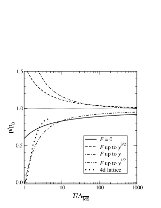
FIG. 1.: The pressure in Eq. (5), with the long-distance part from Eq. (9) included to various loop orders. The 4d lattice results are from the first reference in [1]. It should be noted that they have a normalisation ambiguity at low temperatures $T\mathop{\raise 1.29167pt\hbox{$<$\kern-7.5pt\raise-4.73611pt\hbox{$\sim$}}}T_{c}$ allowing for a small shift of the curve.

The idea of our approach of improving the determination of ${\cal F}_{{\mbox{$\overline{\mbox{\rm MS}}$}}}(x,y)$ is the following. We write

$$\Delta{\cal F}_{{\mbox{$\overline{\mbox{\rm MS}}$}}}(x,y) = \Delta{\cal F}_{{\mbox{$\overline{\mbox{\rm MS}}$}}}(x_{0},y_{0})$$ (11)

$$+\int_{y_{0}}^{y}\!dy\,\biggl{(}\frac{\partial\Delta{\cal F}_{{\mbox{$\overline{\mbox{\rm MS}}$}}}}{\partial y}+\frac{dx}{dy}\frac{\partial\Delta{\cal F}_{{\mbox{$\overline{\mbox{\rm MS}}$}}}}{\partial x}\biggr{)},$$

where $y=y(x)$ is defined in Eq. (2). The partial derivatives are now given by adjoint Higgs field condensates:

$$\frac{\partial\Delta{\cal F}_{{\mbox{$\overline{\mbox{\rm MS}}$}}}}{\partial y}=\biggl{\langle}\frac{{\rm Tr\,}A_{0}^{2}}{g_{3}^{2}}\biggr{\rangle}_{{\mbox{$\overline{\mbox{\rm MS}}$}}}-\biggl{\langle}\frac{{\rm Tr\,}A_{0}^{2}}{g_{3}^{2}}\biggr{\rangle}_{{\mbox{$\overline{\mbox{\rm MS}}$, pert}}},$$ (12)

where $\langle{\rm Tr\,}A_{0}^{2}/g_{3}^{2}\rangle_{{\mbox{$\overline{\mbox{\rm MS}}$, pert}}}$ is the perturbative result up to ${\cal O}(y^{-{\frac{1}{2}}})$, obtained by taking a derivative of Eq. (9) with respect to $y$. In the case of $\partial\Delta{\cal F}_{{\mbox{$\overline{\mbox{\rm MS}}$}}}/\partial x$, a similar relation is obtained but with the condensate $\langle({\rm Tr\,}A_{0}^{2})^{2}\rangle$.

On the other hand, with a computation in lattice perturbation theory, a condensate measured in lattice Monte Carlo simulations can be related to the condensates $\langle{\rm Tr\,}A_{0}^{2}\rangle_{{\mbox{$\overline{\mbox{\rm MS}}$}}}$, $\langle({\rm Tr\,}A_{0}^{2})^{2}\rangle_{{\mbox{$\overline{\mbox{\rm MS}}$}}}$. Due to the super-renormalizable nature of ${\cal L}_{\mbox{3d}}$, such analytic relations can be computed exactly near the continuum limit [17, 18].

Thus, we need to evaluate the condensates on the lattice, transform the result to the $\overline{\mbox{\rm MS}}$ scheme, and perform finally the integration in Eq. (11) numerically. When added to $\Delta{\cal F}_{{\mbox{$\overline{\mbox{\rm MS}}$}}}(x_{0},y_{0})$, we obtain a non-perturbative result, which we can plug into Eq. (5).

What remains is to determine the integration constant $\Delta{\cal F}_{{\mbox{$\overline{\mbox{\rm MS}}$}}}(x_{0},y_{0})$. The idea is that despite the bad convergence shown in  Fig. 1, at high enough temperatures the form of $\Delta{\cal F}_{{\mbox{$\overline{\mbox{\rm MS}}$}}}(x_{0},y_{0})$ is known. Indeed, inspecting the general structure of Eq. (9), we know that

$$\Delta{\cal F}_{{\mbox{$\overline{\mbox{\rm MS}}$}}}(x_{0},y_{0})=\frac{e_{0}}{(4\pi)^{4}}d_{A}C_{A}^{3}\Bigl{(}1+{\cal O}(\frac{x_{0}}{C_{A}},\frac{C_{A}}{4\pi{y_{0}}^{{\frac{1}{2}}}})\Bigr{)}.$$ (13)

Here $e_{0}$, containing an unknown logarithmic dependence on $y_{0}$, represents the famous non-perturbative ${\cal O}(g^{6}T^{4})$ term [10]. Suppose now that we choose $T\equiv T_{0}\sim 10^{11}\Lambda_{\overline{\rm MS}}$, corresponding to $x_{0}=1.0\times 10^{-2}$, $y_{0}=3.86$. Then the higher order terms in Eq. (13) are expected to be subdominant, since $C_{A}/(4\pi{y_{0}}^{{\frac{1}{2}}})\sim 0.1$ and $x_{0}/C_{A}\sim 0.01$, and we only need to know $e_{0}$.

The main error sources of this non-perturbative and unambiguous setup are as follows:

(a) Even though in principle an independent non-perturbative determination of $e_{0}$ is possible for instance by measuring the condensate $\langle{\rm Tr\,}F_{ij}^{2}\rangle$ along the lines in [19], doing this systematically requires a 4-loop computation in lattice perturbation theory, and this is beyond our scope here. Therefore we will treat $e_{0}$ as a free integration constant whose magnitude will be fixed below.

(b) Due to the smallness of $x/C_{A}$, we will also ignore here the term arising from $\partial\Delta{\cal F}_{{\mbox{$\overline{\mbox{\rm MS}}$}}}/\partial x$ in Eq. (11).

(c) The numerical procedure introduces small statistical errors, as well as systematic errors from the extrapolations to the infinite volume and continuum limits.

(d) Finally, we should of course remember that the effective theory ${\cal L}_{\mbox{3d}}$ loses its accuracy when higher order operators not included become important. In fact, for $N_{f}=0$ the QCD phase transition is related to the so called Z(3)-symmetry [11, 20], and this symmetry is not fully reproduced by ${\cal L}_{\mbox{3d}}$ [9, 21], without all the higher order operators. There are many indications, however, that the effective theory should be rather accurate down to low temperatures, $T\sim 2T_{c}$ [6, 9, 13]. Below that, some other effective description may apply (see, e.g., [22]).

Numerical results. After this background, we show in Fig. 2 the difference in Eq. (12), measured with lattice simulations. This result is then used in Eq. (11) to obtain $\Delta{\cal F}_{{\mbox{$\overline{\mbox{\rm MS}}$}}}(x,y)$. When added to Eqs. (9), (5), we obtain Fig. 3. As discussed above, the boundary value at (almost) infinite temperature, determined by $e_{0}$, is for the moment a free parameter.

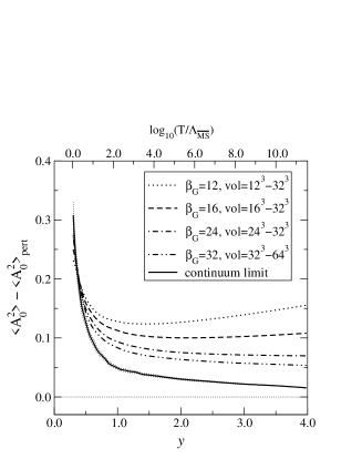
FIG. 2.: The difference in Eq. (12). Here $\beta_{G}=6/(g_{3}^{2}a)$, where $a$ is the lattice spacing, and the continuum limit corresponds to the extrapolation $\beta_{G}\to\infty$.

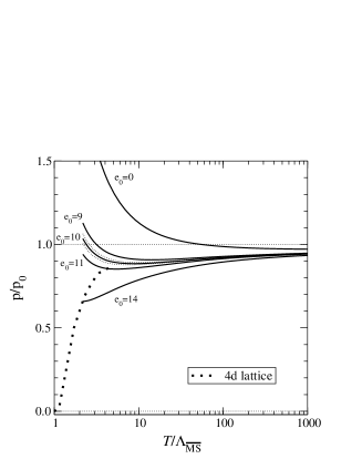
FIG. 3.: The pressure after the inclusion of $\Delta{\cal F}_{{\mbox{$\overline{\mbox{\rm MS}}$}}}(x,y)$ from Eq. (11). Statistical errors are shown only for $e_{0}=10$.

We observe that at low temperatures the outcome depends strongly on the value of $e_{0}$. The correct value would appear to be $e_{0}\approx 10.0\pm 2.0$. Even then, the present results lose their accuracy at $T\sim 5T_{c}$, but seem to work well above this. Exploiting the full power of the dimensionally reduced theory down to its limit $T\sim 2T_{c}$ would also necessitate the inclusion of $\langle({\rm Tr\,}A_{0}^{2})^{2}\rangle$.

Discussion. In 4d lattice simulations, there is a (numerically small) ambiguity in the determination of the pressure, because only pressure differences can be measured, and thus an integration constant has to be specified at low temperatures in a non-perturbative regime. Here we fix the integration constant by starting from the opposite direction, from very high temperatures. This allows to determine all quantities in terms of $T/\Lambda_{\overline{\rm MS}}$ and the number of fermion flavours, without ambiguities. We can also address a huge range of temperatures, unlike 4d simulations which can only go up to $T\sim\mbox{a few}\times T_{c}$.

The result of our procedure is summarised by Eqs. (5)–(12) and Fig. 3. We draw two important conclusions. The first is that the outcome depends strongly on the non-perturbative contribution of order ${\cal O}(g^{6}T^{4})$ [10], as can be observed from the $e_{0}$-dependence in Fig. 3. The value of $e_{0}$ could in principle be determined by a well-defined procedure, although in practice it is a project of considerable technical complication. But our present study provides an estimate for what the result should be. The order of magnitude ${\cal O}(10)$ seems reasonable, since it is known from other contexts such as the Debye mass [13] that non-perturbative constants tend to be large.

The second is that when the large non-perturbative ${\cal O}(g^{6}T^{4})$ term is summed together with the set of all higher order terms determined via $\langle{\rm Tr\,}A_{0}^{2}\rangle$, then these long-distance contributions almost cancel at $T\mathop{\raise 1.29167pt\hbox{$>$\kern-7.5pt\raise-4.73611pt\hbox{$\sim$}}}30\Lambda_{\overline{\rm MS}}$! Indeed, the sum, the curve with $e_{0}\sim 10$ in Fig. 3, does not differ there much from the term ${\cal O}(y^{{\frac{1}{2}}})$ in Fig. 1. For smaller temperatures, $5\Lambda_{\overline{\rm MS}}\mathop{\raise 1.29167pt\hbox{$<$\kern-7.5pt\raise-4.73611pt\hbox{$\sim$}}}T\mathop{\raise 1.29167pt\hbox{$<$\kern-7.5pt\raise-4.73611pt\hbox{$\sim$}}}30\Lambda_{\overline{\rm MS}}$, on the other hand, only our numerical results are trustworthy.

Finally, we also find that although the dependence on the effective scalar self-coupling $x$ is of high perturbative order, in practice it is expected to play a role as one approaches $T_{c}$. Its contribution can be obtained from the condensate $\langle({\rm Tr\,}A_{0}^{2})^{2}\rangle$. To relate this to the $\overline{\mbox{\rm MS}}$ scheme requires again a perturbative 4-loop computation.

Let us end with a philosophical note. When one wants to understand 4d simulation results, one could argue that one should aim at almost fully analytical resummations [14, 15, 16]. However, we suspect that these are unavoidably specific for the particular observable considered: they may work for the entropy or pressure because the result is short-distance dominated, but would fail for instance for Debye screening where long-distance effects are dominant. It seems to us that it may ultimately be more useful to obtain a unified understanding of the relevant degrees of freedom in the system, even if some observables have to be evaluated numerically.

Acknowledgements. This work was supported by the TMR network Finite Temperature Phase Transitions in Particle Physics, EU contract no. FMRX-CT97-0122. We thank the Center for Scientific Computing, Finland, for resources, and D. Bödeker, E. Iancu for discussions.

REFERENCES

- [1] G. Boyd et al, Nucl. Phys. B 469 (1996) 419 [hep-lat/9602007]; A. Papa, Nucl. Phys. B 478 (1996) 335 [hep-lat/9605004]; B. Beinlich, F. Karsch, E. Laermann and A. Peikert, Eur. Phys. J. C 6 (1999) 133 [hep-lat/9707023]; M. Okamoto et al. [CP-PACS Collaboration], Phys. Rev. D 60 (1999) 094510 [hep-lat/9905005].
- [2] P. Arnold and C. Zhai, Phys. Rev. D 50 (1994) 7603 [hep-ph/9408276]; ibid. 51 (1995) 1906 [hep-ph/9410360].
- [3] C. Zhai and B. Kastening, Phys. Rev. D 52 (1995) 7232 [hep-ph/9507380].
- [4] E. Braaten and A. Nieto, Phys. Rev. D 53 (1996) 3421 [hep-ph/9510408].
- [5] P. Ginsparg, Nucl. Phys. B 170 (1980) 388; T. Appelquist and R.D. Pisarski, Phys. Rev. D 23 (1981) 2305.
- [6] S. Nadkarni, Phys. Rev. Lett. 60 (1988) 491; T. Reisz, Z. Phys. C 53 (1992) 169; L. Kärkkäinen et al, Phys. Lett. B 282 (1992) 121; Nucl. Phys. B 418 (1994) 3 [hep-lat/9310014]; Nucl. Phys. B 395 (1993) 733.
- [7] S. Huang and M. Lissia, Nucl. Phys. B 438 (1995) 54 [hep-ph/9411293]; ibid. 480 (1996) 623 [hep-ph/9511383].
- [8] K. Kajantie et al, Nucl. Phys. B 458 (1996) 90 [hep-ph/9508379]; Phys. Lett. B 423 (1998) 137 [hep-ph/9710538].
- [9] K. Kajantie et al, Nucl. Phys. B 503 (1997) 357 [hep-ph/9704416].
- [10] A.D. Linde, Phys. Lett. B 96 (1980) 289.
- [11] D.J. Gross, R.D. Pisarski and L.G. Yaffe, Rev. Mod. Phys. 53 (1981) 43.
- [12] S. Datta and S. Gupta, Nucl. Phys. B 534 (1998) 392 [hep-lat/9806034]; Phys. Lett. B 471 (2000) 382 [hep-lat/9906023].
- [13] M. Laine and O. Philipsen, Nucl. Phys. B 523 (1998) 267 [hep-lat/9711022]; Phys. Lett. B 459 (1999) 259 [hep-lat/9905004]; A. Hart and O. Philipsen, Nucl. Phys. B 572 (2000) 243 [hep-lat/9908041]; A. Hart, M. Laine and O. Philipsen, hep-ph/0004060.
- [14] J.O. Andersen, E. Braaten and M. Strickland, Phys. Rev. Lett. 83 (1999) 2139 [hep-ph/9902327]; Phys. Rev. D 61 (2000) 014017 [hep-ph/9905337]; Phys. Rev. D 61 (2000) 074016 [hep-ph/9908323].
- [15] J.P. Blaizot, E. Iancu and A. Rebhan, Phys. Rev. Lett. 83 (1999) 2906 [hep-ph/9906340]; Phys. Lett. B 470 (1999) 181 [hep-ph/9910309]; hep-ph/0005003.
- [16] A. Peshier, hep-ph/9910451.
- [17] K. Farakos et al, Nucl. Phys. B 442 (1995) 317 [hep-lat/9412091]; M. Laine and A. Rajantie, Nucl. Phys. B 513 (1998) 471 [hep-lat/9705003].
- [18] G.D. Moore, Nucl. Phys. B 493 (1997) 439 [hep-lat/9610013]; ibid. 523 (1998) 569 [hep-lat/9709053].
- [19] F. Karsch, M. Lütgemeier, A. Patkós and J. Rank, Phys. Lett. B 390 (1997) 275 [hep-lat/9605031].
- [20] C.P. Korthals Altes, Nucl. Phys. B 420 (1994) 637 [hep-th/9310195].
- [21] K. Kajantie, M. Laine, A. Rajantie, K. Rummukainen and M. Tsypin, JHEP 9811 (1998) 011 [hep-lat/9811004].
- [22] R.D. Pisarski, hep-ph/0006205.