The impact of atomic precision measurements in high energy physics 111 Talk given at the XVII International Conference on Atomic Physics, ICAP 2000, Florence, June 4-9, 2000
Abstract
In this talk I discuss the relevance of atomic physics in understanding some important questions about elementary particle physics. A particular attention is devoted to atomic parity violation measurements which seem to suggest new physics beyond the Standard Model. Atomic physics might also be relevant in discovering possible violations of the CPT symmetry.
Introduction
The aim of this talk is to review some of the atomic precision measurements in atomic physics leading to precious informations in the realm of high-energy physics. The idea of atomic physics bringing light on the high-energy physics world requires some qualification due to the very different scales of energy involved in the two cases. In fact, typically one has a separation of about six or seven order of magnitude between the two scales and one expects the two physics being almost decoupled. In fact, if we look at some observable, , at a scale , we expect that the observable can be represented in the form
| (1) |
In order to be able to derive informations about the physics at the scale , being at the scale , one starts considering a combination of observables corresponding to the corrections coming from the higher scale
| (2) |
In order to measure one needs either the coefficient being very large in such a way to partially compensate the scale factor, or having an extremely good experimental sensitivity. In this talk I will consider two particular examples of situations where atomic physics can be relevant to high-energy physics, namely Atomic Violation of Parity (APV) and possible violations of the discrete symmetry CPT, that is the product of charge-conjugation, parity and time-reversal. In fact, using heavy atoms like cesium in APV measurements one can get a good enhancement factor. On the other hand, CPT symmetry can be tested by using the extraordinary opportunities offered by the atomic traps in order to obtain a very accurate determination of frequencies.
Atomic Parity Violation in Atoms
In this Section I will discuss mainly the latest determination of the weak charge in atomic cesium and some of its implications in models of physics beyond the Standard Model (SM). The SM has been tested very precisely at machines such as LEP and SLC, where, working at an energy around the mass, one is mainly testing the property of the itself. Therefore, the physics beyond the SM that can be looked for at these machines is the one giving corrections to the -propagator and/or to the couplings of the with fermion-antifermion pairs. Namely, new massive vector bosons, , which mix to the , or new particles running in loops and contributing to the self-energy or to vertex corrections. But consider, for instance, the case of a massive vector boson which does not mix to the , and therefore invisible at LEP (except for tiny radiative corrections). If the is coupled to fermions, in the low-energy limit it gives rise to an effective four-fermi interaction. Therefore, low-energy experiments are complementary to the high-energy ones, and furthermore they are able to measure directly the couplings of the to light quarks; something that at LEP and SLC can be done only in an indirect way. Among the low-energy experiments a particular role is played by the APV experiments, due to the precision almost at the level of the one reached at LEP/SLC.
Let us now recall some feature of APV in atoms. First of all, within the SM the four-fermi parity violating hamiltonian density for nucleons is given by
| (3) |
where
| (4) |
and
| (5) |
Here , , and are the vector and vector-axial couplings of the to the electrons and quarks. For a point-like nucleus with protons and neutrons, the hamiltonian density, in the non-relativistic limit, is given by
| (6) | |||||
| (7) |
where is the momentum of the electron, the total spin of the protons (neutrons) and the electron mass. I have also defined the weak charge of the atom as
| (8) |
Notice that for a heavy atom (large values of ) the matrix element of the first term in is roughly proportional to , one factor coming from , one from the momentum of the electron and the third one from the wave function evaluated at the origin. This coherence effect was noticed by Bouchiat and Bouchiat bouchiat2 and it provides, in the case of cesium () an enhancement factor of about , more or less what is necessary in order to compensate for the decoupling factor from the scales mentioned in the Introduction.
In order to get a rough idea of the bounds on new physics that can be obtained by a measurement of with a given sensitivity, we parametrize the new physics contribution to by a four-fermi effective interaction musolf
| (9) |
If we assume , for a sensitivity one gets a bound
| (10) |
If new physics is strongly interacting (), then , whereas in the weakly interacting case () we get . In any case we see that at 1% level of sensitivity, is able to test new physics for scales greater than 1 .
In APV measurements one looks at optical transitions between a pair of states mixed by and a state of the same nominal parity as . The mixing of the two eigenstates of parity is given by
| (11) |
where is the splitting between the two levels. If I denote by and the amplitudes for the two unperturbed transitions and , the transition probability, after the mixing, is given by
| (12) |
The choice of the sign depends on the helicity of the photon which is emitted or absorbed in the transition. In the actual experiment on cesium one measures the circular dichroism, that is the asymmetry for the absorption cross-section
| (13) |
Of course, the PV amplitude is proportional to the mixing parameter and therefore measuring one can get the matrix element of the PV hamiltonian. These ideas have been applied in particular to the transition in atomic cesium bouchiat ; boulder1 ; boulder2 , but also to other atoms as thallium thallium . The typical value of is , but there is a strong background which can be overcomed by letting the PV amplitude to interfere with a large electro-induced (Stark) transition. Eventually one extracts from the experiment the matrix element of which is proportional to times an atomic form factor which must be evaluated theoretically in order to extract the value of the weak charge. Therefore the measurement must be coupled with theoretical calculations of similar accuracy in order to get a precise determination of . In the case of atomic cesium the calculation of was performed independently by two groups dzuba ; blundell . This calculation is not an easy task, as one has to use many-body perturbation theory coupled with Hartree-Fock techniques. The theoretical errors are quite difficult to estimate. The authors of Refs. dzuba ; blundell did their estimate by looking at the differences between the theoretical and the experimental values of parity conserving quantities as dipole matrix elements and hyperfine splittings for the , , and states. In this way the error was obtained. After the new measurement of the weak charge of the cesium by the Boulder group boulder2 , which improved the accuracy of the previous experiment boulder1 by more than a factor five, Bennett and Wieman bennett re-examined the theoretical errors on . In fact, since the time of the previous estimate there have been a number of new and more precise measurements of the quantities of interest. The result is that now the agreement is much better than before, and as a consequence Bennett and Wieman got the estimate . It should be noticed that there is a third element which contributes to the extraction of from the data. This is the Stark mixing-induced electric dipole moment amplitude, . The experiments in Refs. bouchiat ; boulder1 were using a theoretical determination of . In boulder2 the ratio has been measured. The off-diagonal magnetic dipole moment induced by the hyperfine interaction is well known empirically and it is possible to extract a precise value for . However, in a contribution to this Conference dzuba2 , the matrix element has been accurately calculated with the result that the empirical formula for it should be corrected by a factor of 0.24% increasing the discrepancy with the SM (see later). I would like also to comment about some possible neglected contribution in the evaluation of the atomic form factor. It has been pointed out in ref. pollock that there could be a contribution arising from the difference of neutron and proton spatial distributions inside the nucleus. This contribution turns out to be very difficult to estimate, in fact it is quite model dependent. Most probably it could introduce a further error on of about 0.3. This would not change the conclusions in a very significant way. Another point has been raised recently in ref. derevianko . This author argues that the contribution from the Breit interaction (exchange of a transverse photon between two electrons) could have been underestimated. The Breit interaction contribution to the atomic form factor was estimated in dzuba and it was found to be very small. However in ref. derevianko it is found that the total effect, taking into account also second and third order contributions, is about twice the first order effect. As a consequence, if ”all” the higher order contributions could be shown to be negligible, the experimental measure would reconcile with the SM expectation for . However, see also ref. kozlov .
To conclude this analysis I think that an evaluation of the atomic form factor by taking into account the next order in the many-body perturbative theory is highly desirable in order to settle the question. In any case I find of some interest to assume that the theoretical error is indeed at the level of in order to see which are the possible implications of the APV in high-energy physics.
I can start now to discuss the experimental results on . It is interesting to recall the value obtained in boulder1 combined with the theoretical determination of dzuba ; blundell
| (14) |
The total error of these measurement on is at 2.5% level of accuracy that, at that time, was comparable with the sensitivity obtained at LEP1. In fact, this determination of lead to the first indication that technicolor models, in their most simple version obtained from scaling of QCD, could not possibly fit the data. The new experimental result on boulder2 combined with the new determination of the theoretical error bennett gives
| (15) |
A result at 0.6% level of accuracy. On the theoretical side, can be expressed as marciano
| (16) |
including hadronic-loop uncertainty. I use here the variables (i=1,2,3) of ref. altarelli , which include the radiative corrections, in place of the set of variables , and originally introduced in ref. peskin . In the above definition of I have explicitly included only the Standard Model (SM) contribution to the radiative corrections. New physics (that is physics beyond the SM) contributions are represented by the term . Also, I have neglected a correction proportional to . In fact, as well known marciano , due to the particular values of the number of neutrons () and protons () in cesium, the dependence on almost cancels out. For a top mass of 175 and the value of is given by altarelli2
| (17) |
For , corresponding roughly to the lower experimental bound from direct search at LEP2 higgs , one gets
| (18) |
giving rise to a deviation of about . Furthermore, for increasing mass of the Higgs the discrepancy increases. Therefore, if we assume as being correct the experimental result, the theoretical evaluation of and the evaluation of the theoretical errors, we are forced to conclude that the SM is disfavored at 99% CL.
We can draw another conclusion, that is, that in order to explain the data on we need new physics not constrained by the LEP and SLC data. In fact, as an example let me consider a type of new physics visible at LEP as, for instance, contributing to the self-energy of the , the so called oblique corrections. In such a case one can write , and in order to compensate for the discrepancy on one needs
| (19) |
whereas from LEP and SLC data one can determine the sum
| (20) |
Therefore one gets , one order of magnitude too small to explain the data on .
I would like also recall the experimental result of APV on Thallium thallium
| (21) |
This result is not as precise as the one on , and in fact the total error is about 3%. At this level it is perfectly compatible with the SM prediction
| (22) |
A new experiment on cesium is being planned in Paris but the experimental sensitivity is going to be lower than the one obtained in Boulder.
In Berkeley and Seattle there are plans for isotope ratio measurements. In this case the dependence on the atomic form factor would go away eliminating the theoretical error. However these ratios depend on the variation of the neutron density along the isotope chain. This would introduce errors at least twice as big as the experimental ones chen .
We are now in the position of discussing the implications of eq. (18) on new physics. Assuming that the contribution of new physics, , is such to reproduce the experimental results, we can make use of eqs. (15) and (16) to write casalbuoni
| (23) |
For at a 95% CL we find
| (24) |
Notice that the lower positive bound arises since the SM (corresponding to ) does not fit the experimental value of at this CL value. This is quite important since it implies an upper bound on the scale of new physics. For the same reason new physics with a contribution is not allowed. Also notice that lower and upper bounds both increase for increasing Higgs mass.
Contact interactions from compositness.
A typical four-fermi operator in composite models contributing to the PV lagrangian is langacker ; casalbuoni
| (25) |
The effect of this interaction is to modify the coefficients
| (26) |
where, since composite models correspond to strongly interacting new physics, we have assumed . From
| (27) |
we see that the negative sign for the operator (25) is excluded. For the positive sign we get the bounds
| (28) |
The typical lower bound from high energy physics is about 3.5 PDG .
Extra-dimension models.
In ref. pomarol a minimal extension to higher dimensions of the SM, with extra dimensions compactified, was considered. In this model the fermions live in a 4-dimensional subspace, the wall, whereas the gauge bosons live in the full D-dimensional space, the bulk. In general, there might be two Higgs fields, one living in the bulk, , and the other living on the wall, . The propagation of the gauge fields in the bulk is equivalent to the exchange of an infinite tower of Kaluza-Klein (KK) excitations with increasing mass. For example, for , , , with the compactification radius. If only the Higgs field is present, the ordinary gauge bosons do not mix with the KK resonances and it is easy to see that the contribution of these modes to is negative casalbuoni2 . Therefore the model does not fit the data on . For the more general case of both Higgs fields present it has been shown casalbuoni2 that the LEP/SLC and experimental data are not compatible among them at 95% CL.
Extra models.
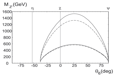
The implications of models with an extra neutral vector boson for APV have been considered in the literature for quite a long time qwz ; casalbuoni2 ; erler . The has couplings comparable to the ones of the in the SM and therefore this is an example of weakly interacting new physics. There is a continuum of such models characterized by an angle . To any value of it corresponds a different model. The 95% CL regions allowed by , in the plane , for different values of the Higgs mass, are shown in Fig. 1. In deriving these Figures the assumption of zero mixing between and has been made. In the Figure are also shown three popular models: (), (), (). We see that the and the models are not allowed by the data. The direct search at the Tevatron for a within the model gives a direct lower bound at 95% CL, (a similar bound holds for all these models) . Therefore this model is compatible with the data. A recent best fit to all the data (including APV) gives for the model the following results erler , and a mixing angle compatible with zero, .
Atomic physics and CPT violation
The CPT theorem is one of the fundamental results in local relativistic field theories. Therefore the idea of possible violations of this theorem implies that some of the axioms of these theories should be reviewed. Let me recall here the exact statement of the theorem cpt : In a field theory satisfying
-
1.
Locality
-
2.
Lorentz invariance
-
3.
Analiticity of the Lorentz group representations in the boost parameters
the CPT transformation is a symmetry of the theory itself.
The first two conditions say that one is dealing with a local relativistic field theory, whereas the third one is satisfied in any finite-dimensional representation of the Lorentz group. It is interesting to notice that unitary representations fail to be analytic and as a consequence the CPT theorem can be violated in this case. The first example of this situation dates back to Majorana majorana when he formulated a first order wave equation without negative-energy solutions. He was able to do that by making use of a unitary infinite-dimensional representation of the Lorentz group. Since this theory does not contain antiparticles the CPT symmetry is broken. However, the quarks and leptons described by the SM belong to finite-dimensional representation of the Lorentz group and therefore this does not seem a possible way to break the theorem. It seems also very hard to give up locality, since it guarantees the microcausality of the theory. Therefore, the only sensible way to avoid the consequences of the CPT theorem in a local field theory seems to break Lorentz invariance. A situation of this type could arise at a more fundamental level as in string theory, where it is possible that Lorentz invariance is spontaneously broken around the Planck mass, kostelecky1 . One can take into account these effects by writing down a local effective lagrangian with Lorentz and CPT breaking terms. These terms can be written as an expansion in derivatives over the Planck mass. For instance, considering a single fermion, the violating term can be written as
| (29) |
I have used a somewhat symbolic notation where stays for a generic combination of Dirac matrices and is a constant tensor and I take the mass dimensions of as . Furthermore I will assume the same internal symmetries as in the SM, that is kostelecky2 ; kostelecky3 . Since the breaking terms should vanish in the limit also for , I will require
| (30) |
where is some low-energy mass scale parameter. We see that the relevant terms are the ones with and , and therefore the resulting theory preserves the renormalizability property.
Let me now consider a single fermion interacting with the electromagnetic field. One adds to the standard QED lagrangian the following two terms
| (31) |
and
| (32) |
where , with the electric charge of the fermion. There are other possible terms with , but they are not compatible with the symmetries of the SM and therefore they should be suppressed. The following orders of magnitude are expected
| (33) |
The terms in violate Lorentz invariance, since all the tensors in eq. (33) are constant ones. However only the terms proportional to and violate CPT symmetry since , and are CPT odd, whereas the other covariant terms are CPT even. Therefore, in the following I will take into consideration only . Notice also that when dealing with a single fermion the term in does not have physical meaning since we can write , showing that is a trivial gauge background field. Of course, the situation changes when dealing with different fermions having different ’s. From eq. (33) we expect that the order of magnitude of the CPT and Lorentz breaking terms is given by for , where is the electron mass and is the electroweak symmetry breaking scale. Lorentz and CPT breaking terms could appear also in the photon part of the total lagrangian. This instance is discussed thoroughly in the second paper of ref. kostelecky2 , but I will not consider it in this talk.
Here I want to illustrate some atomic physics experiment about CPT violation. But before doing that let me just give a list of other existing or planned experiments about the violation of this fundamental symmetry
-
•
mass difference. This experiment gives the best high-energy result PDG
(34) -
•
Experiments on neutral meson oscillations to be done at meson factories kostelecky4 .
-
•
Experiments on muons kostelecky5 .
-
•
Experiments with spin-polarized solids bluhm1 .
-
•
Experiments from clock-comparison kostelecky6 .
CPT violation may have also some relevance for baryogenesis and this subject has been discussed in ref. bertolami .
Let me now consider atomic physics experiments for testing CPT using atomic traps. Several of these experiments have been performed by confining single particles or antiparticles in a Penning trap for a long time. These experiments have a very high precision, of order or better, whereas the precision in experiments about mesons (see eq. (34)) is much lower, of order . I recall here the comparison of the electron and positron gyromagnetic ratios, , obtained measuring their cyclotron and anomaly frequencies (see later), which gives the figure of merit dyck
| (35) |
Measuring the proton and antiproton cyclotron frequencies, one can get their charge-to-mass ratios. gabrielse
| (36) |
Analogously, from the charge-to-mass ratio for electron and positron schwinberg
| (37) |
As we see the relevant figures of merit are much bigger than the one for the mass difference , although, as noticed, these measurements are about six order of magnitude more sensitivity than the one leading to (34). In ref. bluhm2 it has been argued that these figures of merit could not be the relevant ones in testing CPT breaking. In fact, within the approach presented here, at the lowest order in the CPT violating parameters, one has , and similarly the charge-to-mass ratios do not depend on these parameters bluhm2 . To review this point, let me start by the Dirac equation for an electron or a proton including the breaking terms contained in (of course, the breaking parameters may depend on the type of particle one is considering)
| (38) |
In a Penning trap the radial confinement is obtained through a strong axial magnetic field, whereas the axial confinement is obtained by a quadrupole electric field. The main corrections due to the CPT and Lorentz breaking parameters are obtained by taking as the four-potential for a constant magnetic field. Then, to obtain the energy shifts generated by the breaking parameters one makes use of the relativistic Landau levels wave functions and the expressions containing the full QED corrections for the unperturbed levels bluhm2 ; bluhm3 . However, the underlying physics can be understood quite simply recalling the expression for the non-relativistic Landau levels
| (39) |
The cyclotron and anomalous frequencies are obtained comparing two Landau levels with different quantum number and with the same and opposite spin configurations respectively
| (40) |
The relevant CPT and Lorentz breaking corrections to the energy levels are given by bluhm3
| (41) |
where we have taken the third axis along the magnetic field of the trap. The frequencies for the antiparticles that we need according to the CPT theorem are the ones with inverted spin, therefore
| (42) |
We get
| (43) |
We recall that these equations hold only at the first order in the breaking parameters and also that the usual relation does not hold here since, as noted before, the gyromagnetic ratios do not change at the lowest order.
Since the observables that are measured in a Penning trap are the anomalous and cyclotron frequencies, it seems natural to introduce figures of merit related to these observables. A such figure of merit for CPT violation is bluhm2
| (44) |
where . For a weak magnetic field one gets
| (45) |
A new analysis of the 1987 experiment by Dehmelt et al. dyck has been done recently in ref. dehmelt obtaining the following bound
| (46) |
However, the vector is absolutely constant and as such it rotates with a diurnal period of 23 h and 56 m, when seen in the laboratory frame wich is fixed with respect to the earth. This effect might have given rise to non favorable situations during the observation, and therefore the bound has been a bit relaxed dehmelt
| (47) |
In the case of proton and atiproton there is no experiment at the moment. Assuming an experimental sensitivity analogous to the electron positron case (meaning ) one gets bluhm3
| (48) |
The last case I consider is the spectroscopy of free or magnetically trapped hydrogen () and antihydrogen (). This is interesting since the two-photon transition has been measured with a precision of udem in a cold atomic beam of and with a precision of in trapped cesar . However for the free case the dependence of the transition on the CPT and Lorentz breaking parameters is suppressed by a factor , since the and levels shift by the same amount at the leading order in the breaking bluhm4 . Consider now the spectroscopy of and in a magnetic field . In the basis the four and hyperfine Zeeman levels are, for
| (49) |
with . Transitions of the type have leading-order sensitivity to Lorentz and CPT violation, but they are field-dependent. As a consequence there is a problem connected with the broadening of the lines due to trapping field inhomogeneities.
Consider now hyperfine transitions in the ground state. Again there is the problem of the Zeeman broadening. However one can try to eliminate the frequency dependence on (at lowest order) by choosing a field independent transition point bluhm4 . For the state is highly polarized (). Then the effect on the transition of the CPT and Lorentz violating parameters is . Therefore by putting the corresponding figure of merit can be defined as
| (50) |
Attaining a resolution of , one would get bluhm4
| (51) |
Conclusions
In this talk I have reviewed some important consequences of atomic physics measurements in the domain of high-energy physics. In particular APV in cesium could be the first real indication of new physics beyond the SM. The atomic physics tests of the CPT symmetry are already at a spectacular level of sensitivity, and the future experiments on and could give bounds well below the one expected from string theory.
References
- (1) Bouchiat M.A. and Bouchiat C.C., Phys. Lett. B48, 111 (1974); J. Phys. 35, 899 (1974).
- (2) Ramsey-Musolf M.J., physics/0001250, (2000).
- (3) Bouchiat M.A., Guena J., Hunter L. and Pottier L., Phys. Lett. B117, 358 (1982).
- (4) Noecker M.C., Masterson B.P. and Wieman C.E., Phys. Rev. Lett. 61, 310 (1988).
- (5) Wood C.S., Bennett S.C., Cho D., Masterson B.P., Roberts J.L., Tanner C.E. and Wieman C.E., Science 275, 1759 (1999).
- (6) Vetter P.A., Meekhof D.M., Majumder P.K., Lamoreaux S.K. and Fortson E.N., Phys. Rev. Lett. 71, 3442 (1993); Edwards N.H., Phipp S.J., Baird E.G., Nakayama S., Phys. Rev. Lett. 74, 2654 (1995).
- (7) Dzuba V.A., Flambaum V.V., Silvestrov P. and Sushkov O., Phys. Lett. A141, 147 (1989).
- (8) Blundell S.A., Johnson W.R. and Sapirstein J., Phys. Rev. Lett. 65, 1411 (1990).
- (9) Bennett S.C. and Wieman C.E., Phys. Rev. Lett. 82, 2484 (1999).
- (10) Dzuba V.A., Flambaum V.V. and Ginges J.S.M., contribution A11 to this meeting, Conference Abstracts, eds. F. Fusi and F. Cervelli. See also Dzuba V.A. and Flambaum V.V., physics/0005038, (2000).
- (11) Pollock S.J. and Welliver M.C., Phys. Lett., B464, 177 (1999).
- (12) Derevianko A. physics/0001046, (2000); Derevianko A., hep-ph/0005274, (2000).
- (13) Kozlov M.G., Porsev S.G. and Tupitsyn I.I., physics/0004076, (2000) and contribution A15 to this meeting, Conference Abstracts, eds. F. Fusi and F. Cervelli.
- (14) Marciano W.J. and Rosner J.L., Phys. Rev. Lett. 65, 2963 (1990); Altarelli G., Lectures given at the Les Houches Summer School: Particles In The Nineties, 30 Jun - 26 Jul 1991, Les Houches, France.
- (15) Altarelli G., Barbieri R. and Jadach S., Nucl. Phys. B369, 3 (1992); Altarelli G., Barbieri R. and Caravaglios F. Nucl. Phys. B405, 3 (1993); ibidem Phys. Lett. B349, 145 (1995).
- (16) Peskin M.E. and Takeuchi T., Phys. Rev. Lett. 65, 964 (1990); ibidem Phys. Rev. D46, 381 (1991).
- (17) Altarelli G., Barbieri R. and Caravaglios F., Int. J. Mod. Phys. A13, 1031 (1998), and updating of these results as communicated to me by Dr. Caravaglios.
- (18) The actual experimental lower bound on the Higgs mass is 107.9 at 95% CL, see: ALEPH, DELPHI, L3 and Opal Collaborations. The LEP Working group for Higgs boson searches, CERN-EP-2000-055, April 2000.
- (19) Pollock S.J., Fortson E.N. and Wilets L., Phys. Rev. C46, 2587 (1992); Chen B.Q. and Vogel P., Phys. Rev. C48, 1392 (1993).
- (20) Casalbuoni R., De Curtis S., Dominici D. and Gatto R., Phys. Lett. B460, 135 (1999).
- (21) Langacker P., Phys. Lett. B256, 277, (1991).
- (22) Particle Data Group, Caso C. et al., Eur. Phys. J. C3, 1 (1998).
- (23) Pomarol A. and Quiros M., Phys. Lett. B438, 255 (1998); Delgado A., Pomarol A. and Quiros M., Phys. Rev. D60, 95008 (1999); Masip M. and Pomarol A. Phys. Rev. D60, 96005 (1999).
- (24) Casalbuoni R., De Curtis S., Dominici D. and Gatto R., Phys. Lett. B462, 48 (1999).
- (25) Amaldi U. et al., Phys. Rev. D36, 1385 (1987); Marciano W.J. and Rosner J.L., Phys. Rev. Lett. 65, 2963 (1990); Altarelli G. et al. Phys. Lett. B261, 146 (1991); Mahantappa K.T. and Mohapatra P.K., Phys. Rev D43 3093 (1991); Rosner J.L., Phys. Rev. D61, 016006 (2000). In these papers it is also possible to find a complete list of references to the models.
- (26) Erler J. and Langacker P., Phys. Rev. Lett. 84, 212 (2000).
- (27) Streater R.F. and Wightman A.S., PCT, spin and statistics and all that, edited by W.A. Benjamin, Inc., New York, Amsterdam, 1964.
- (28) Majorana, E., Il Nuovo Cimento 9, 335 (1932). This paper is in italian and it was translated in english by Fradkin E.S., AJP 34, 314 (1966).
- (29) Kostelecký V.A. and Potting R., Nucl. Phys. B359, 545, (1991); ibidem, Phys. Lett. B381, 389, (1996); Kostelecký V.A. and Samuel S., Phys. Rev. Lett. 63, 224, (1989); ibidem, Phys. Rev. Lett. 66, 1811, (1991); ibidem, Phys. Rev. D39, 683, (1989); ibidem, Phys. Rev. D40, 1886, (1989).
- (30) Colladay D. and Kostelecký V.A., Phys. Rev. D55, 6760, (1997); ibidem, D58, 116002, (1998).
- (31) For a recent review of the results on this subject, see Kostelecký V.A., hep-ph/0005280, (2000).
- (32) Kostelecký V.A., Phys. Rev. Lett. 80, 1818, (1998).
- (33) Bluhm R., Kostelecký V.A. and Lane C.D., Phys. Rev. Lett. 84, 1098, (2000).
- (34) Bluhm R. and Kostelecký V.A., Phys. Rev. Lett. 84, 1381, (2000).
- (35) Kostelecký V.A. and Lane C.D., Phys. Rev. D60, 116010, (1999).
- (36) Bertolami O. et al., Phys. Lett. B395, 178 (1997).
- (37) Van Dyck R.S. Jr., Schwinberg P.B. and Dehmelt H.G., Phys. Rev. Lett. 59, 26 (1987); ibidem Phys. Rev. D34, 722 (1986). For a review of the principles of the Penning trap, see: Brown L.S. and Gabrielse G. Rev. Mod. Phys. 58, 233 (1986).
- (38) Gabrielse G. et al., Phys. Rev. Lett. 82, 3198 (1999).
- (39) Schwinberg P.B., Dyck R.S. Jr. and Dehmelt H.G., Phys. Lett. A81, 119 (1981).
- (40) Bluhm R., Kostelecký V.A. and Russell N., Phys. Rev. Lett. 79, 1432 (1997).
- (41) Bluhm R., Kostelecký V.A. and Russell N., Phys. Rev. D57, 3932 (1998).
- (42) Dehmelt H., Mittleman R., Van Dyck R.S. Jr. and Schwinberg P., Phys. Rev. Lett. 83, 4694 (1999).
- (43) Udem T. et al., Phys. Rev. Lett. 79, 2646 (1997).
- (44) Cesar C.L. et al., Phys. Rev. Lett. 77, 255 (1996).
- (45) Bluhm R., Kostelecký V.A. and Russell N., Phys. Rev. Lett. 82, 2254 (1999).