CHIRAL QCD: BARYON DYNAMICS 

Abstract

I review the consequences of the chiral symmetry of QCD for the structure and dynamics of the low–lying baryons, with particular emphasis on the nucleon.

FZJ-IKP(TH)-2000-17

1 A short guide through this long essay

There are many approaches which relate baryon structure and properties to QCD in the non–perturbative regime, i.e. at energies, where the running coupling constant $\alpha_{S}(Q^{2})$ is sufficiently large to render conventional perturbation theory doubtful. In this regime, quarks and gluons are confined within hadrons. In addition, the low–energy dynamics is severely constrained by the spontaneously and explicitly broken chiral symmetry of QCD. To account for these facts, many models have been invented which emphasize a certain aspect of the underlying theory. To pick one example, let me just point out that the bag model describes baryons made of bagged (confined) quarks in a simple and appealing picture, with the confinement due to the difference of the pressure in the vacuum and in the baryon state. However, in such a framework one has very little control over the approximations involved. Another type of approaches can be considered more ambitious in that they only try to implement basic principles underlying QCD at the expense of some parameters which have to be determined from data and which parameterize our ignorance of going directly from QCD to the baryon states. One of these approaches are the sum rules, championned by Boris Ioffe and his collaborators for baryons. Here, the non–perturbative vacuum structure is given in terms of a string of quark, gluon and mixed condensates, which are matched to the operator product expansion of the n–point function under consideration. A detailed discussion of this framework can be found in the contribution by Colangelo and Khodjamirian to this Festschrift. In this essay, I will be concerned with a very different approach. In a certain sense it is more general than QCD since it solely explores the consequences of the spontaneously and explicitly broken chiral symmetry for the structure and dynamics of the low–lying baryons. The underlying framework is an effective field theory based on asymptotically observable states, here the Goldstone bosons and the matter fields. The basic ideas of the Goldstone boson dynamics are discussed in detail by Heiri Leutwyler in this book, so I will focus on the picture of baryon structure at low energies as it follows from the chiral QCD dynamics. This picture completely masks the quark and gluon degrees of freedom clearly seen at high energies, which is not that surprising since in many physical systems collective excitations govern the low energy dynamics. The Goldstone bosons of QCD can be thought off as such collective excitations and the baryons essentially as sources surrounded by a cloud of these. As I will show, this meson cloud picture has far–reaching consequences for the baryon structure and is well established by now through a series of precision experiments. In any case, this non–perturbative regime of QCD is most challenging to theorists and it is therefore not surprising that the progress is slow but steady. Still, the field has matured to a point that truely quantitative tests of chiral symmetry breaking can be performed, as I will detail in the following sections. A basic discussion of hadron effective field theory is given in in section 3. Many applications for the two– and three–flavor cases are discussed in sections 4 and 5, respectively. No attempt to achieve completeness is made and only material available before July 2000 was included. Before embarking on any of these issues in detail, I will give a very pedestrian type of introduction in section 2 trying to outline the basic ideas and the emerging picture in a fairly descriptive way. This should allow the beginner to catch the essential concepts without being overwhelmed by heavy machinery. The reader more interested in results or derivations might want to skip this section. More precisely, a short review of the chiral symmetry of QCD is given in section 2.2, followed by a discussion on how one can derive dynamics from symmetry in section 2.3 and some remarks on the physical picture emerging for the structure of the baryons in section 2.4.

2 From symmetry to dynamics

2.1 Some introductory remarks

The spectrum of the low–lying mesons reveals some interesting features. Starting at the mass of the rho meson, $M_{\rho}\simeq 770\,$MeV, a whole zoo of scalar, vector, pseudoscalar and axial states is observed. These states come in multiplets (octets or nonets) organized in terms of a flavor SU(3). The average mass of these lowest multiplets is $M_{M}\simeq 1\,$GeV. Below, there are nine pseudoscalar states which are suspiciously light, in particular the three pions ($\pi^{+},\pi^{0},\pi^{-}$), $M_{\pi}/M_{M}\simeq 1/7$, the kaons ($K^{+},K^{-},K^{0},\overline{K^{0}}$) and the eta with $M_{K}\simeq M_{\eta}\simeq M_{M}/2$. As explained below, these nine particles can be considered as the Pseudo–Goldstone bosons related to the spontaneous breakdown of the chiral symmetry of QCD. Due to Goldstone’s theorem, their interactions vanish as the momentum transfer goes to zero. In fact, this statement does not only hold for interactions between Goldstone bosons, like e.g. for low energy elastic pion–pion scattering, but also for Goldstone bosons interacting with “matter” fields. Here, by matter I denote any particle which is not a Goldstone boson, in particular also the nucleon. As a consequence, it follows that the pion–nucleon interaction at low energies has to be weak and thus paves the way for a systematic expansion of such low energy processes in terms of small external momenta (or derivatives). Clearly, the mass scale of these matter fields is not related to chiral symmetry and thus sets a natural boundary for such type of approach. This is exactly the situation which allows one to make use of the concept of effective field theory, namely that one has a scale separation. In the simplified world of exactly massless up, down and strange quarks, the Goldstone bosons would be massless and the strong interactions could be described by a theory with a mass gap, the height of this gap given by the lowest resonance mass. More generally, one can identify the scale of chiral symmetry breaking to be of the order of 1 GeV. The small expansion parameters to be dealt with are momenta divided by this scale and quark (meson) masses divided by it. This leads in a very natural way to chiral perturbation theory and a plethora of predictions for reactions involving pions, kaons, etas and also external fields like e.g. photons. These considerations can be extended in a fairly straightforward manner to the ground state octet of baryons, since these can not further decay. Stated differently, one can extend the effective field theory to include these massive degrees of freedom and still have a systematic power counting. This can most easily be understood in terms of relativistic quantum mechanics. By construction, external momenta impinging on such a baryon are small compared to its mass because $m_{B}\simeq 1\,$GeV, which is close to the scale of chiral symmetry breaking. Therefore, one is dealing with a Dirac equation for a very heavy fermion, which can be treated in a systematic fashion by means of a Foldy–Wouthuysen transformation. This allows to shuffle the large fermion mass into a string of local operators with increasing powers in the inverse of the mass. By the same argument, it becomes clear why the treatment of excited states is in general out of the realm of such a systematic expansion. When an excited state decays, the energy release is most often too large (one exception will be discussed below). I will now try to explain these concepts in simple terms, without any mathematical rigor.

2.2 Chiral symmetry of QCD

It is instructive to describe chiral symmetry using only elementary mathematics.[1] For that, consider an idealized world in which the up, down and strange quarks are massless. This is the so–called chiral limit of QCD. For each quark, there is a right–handed (RH) helicity state with the spin parallel to the momentum and a left–handed (LH) helicity state with the spin antiparallel to the momentum. All interactions in the QCD Lagrangian are the same for left and right helicity and, furthermore, do not flip helicity chiefly because gluons couple to color and not to flavor. Therefore, a left–handed massless quark will always remain left–handed and similarly, a right–handed massless state stays right–handed. Thus, one has two separate worlds, a LH world and a RH world. These two worlds do not communicate. Since each flavor is massless and has the same QCD couplings, there exists a separate flavor SU(3) in each world, i.e. we can perform independent SU(3) rotations on the right– and the left–handed quarks. This global symmetry is called SU(3)${}_{\rm L}\times$SU(3)_R, the chiral symmetry. Let us now get closer to the physical situation and add a common mass to the quarks. Clearly, one can no longer maintain the separate invariances under left– and right–handed rotations. For a massive particle with a given handedness, one can always perform a boost to a frame moving in the other direction, such that the particle changes say from being left– to right–handed. Therefore, by simple kinematics, the two worlds are no longer separated and one has no longer two independent SU(3) symmetries. However, there remains an invariance under common L+R rotations, with the corresponding SU(3)_V symmetry (since the sum of left– and right–handed generators leads to a vector). If for some reason the mass is small, the SU(3)${}_{\rm L}\times$SU(3)_R symmetry could be an approximate symmetry allowing to treat the mass term as a perturbation. In the real world, all light quark masses are different, so the SU(3)_V is really broken into a direct product of three U(1) symmetries. However, to the extent that the mass differences are small, one can consider the SU(3)_V as an approximate symmetry and treat these mass differences as perturbations. To see this in more detail consider the triplet of quark fields

$$q=\left(u,d,s\right)^{T}~{},$$ (1)

where ${}^{\prime}T^{\prime}$ means transposed, and the left and right projection operators

$$P_{L}={1\over 2}(1+\gamma_{5})~{},\quad P_{R}={1\over 2}(1-\gamma_{5})~{},$$ (2)

with

$$P_{L}^{2}=P_{L}~{},\quad P_{R}^{2}=P_{R}~{},\quad P_{L}\,P_{R}=0~{},\quad P_{L}+P_{R}=I~{},$$ (3)

with $I$ the unit matrix such that

$$q_{L}=P_{L}\,q~{},\quad q_{R}=P_{R}\,q~{},\quad q=q_{L}+q_{R}~{}.$$ (4)

For massless particles, the $P_{L,R}$ project out the helicity of the particle. For massive particles, the $P_{L,R}$ are still projection operators but do not give exactly the helicity. Therefore, one introduces the word chirality (or handedness). In terms of the chiral quarks, the Dirac part of the QCD Lagrangian takes the form

$${\cal L}_{\rm QCD,fermions} = \bar{q}(iD\!\!\!\!/-m)q$$ (5)

$$= \bar{q}_{L}\,iD\!\!\!\!/\,q_{L}+\bar{q}_{R}\,iD\!\!\!\!/\,q_{R}+\bar{q}_{L}\,m\,q_{R}+\bar{q}_{R}\,m\,q_{L}~{},$$

which shows the advocated feature that for $m=0$, the left– and right–handed worlds decouple so that the QCD Lagrangian is invariant under $q_{L}\to Lq_{L}$, $q_{R}\to Rq_{R}$ for $L,R\in$ SU(3)_L,R. The mass term mixes the different chiralities as explained before. Since such flavor transformations do not affect the gluon fields, there was no need of spelling out explicitly how these spin–1 fields are hidden in the gauge covariant derivative $D_{\mu}$ and have their own Yang–Mills Lagrangian. Since SU(3) has 8 generators, Noether’s theorem tells us that the massless theory should have 16 conserved currents and charges, eight constructed from bilinears of the left–handed fermions and eight from the right–handed ones. Since we can also combine L+R to give a vector and L-R to give an axial–vector, one can equally well talk of eight conserved vector and eight conserved axial–vector currents. The vector currents and charges are the usual SU(3)_V = SU(3)_flavor ones which are the basis of the hadron multiplet structure (the “eightfold way”). With the additional eight axial generators, one would expect larger multiplets. This can be seen as follows. Performing an axial rotation on a single particle state leads to a different state with exactly the same mass but of opposite parity because $[{\rm H_{QCD}},Q_{5}^{a}]=0$, where $Q_{5}^{a}$ is any one of the eight axial generators. Such a doubling of hadron states is not observed in nature, e.g. there exists no state with the same mass as the proton but opposite parity. Consequently, this larger symmetry must be hidden. This phenomenon is also called spontaneous symmetry breaking. It is important to realize that although the full symmetry is not present in the spectrum, it still allows one to make powerful predictions.

2.3 Dynamical consequences of chiral symmetry

The most important and also most difficult step in the understanding of dynamical symmetry breaking is why one can make predictions at all. Such predictions will be at the heart of this article. So let us be more general and consider a Lagrangian which is invariant under some symmetry but allow for a continuous family of ground states. These are related to each other by the symmetry but are assumed not to be invariant under it individually. This can be illustrated in some classic examples. First, consider a field theory of a complex scalar field $\phi$,

$${\cal L}=|\partial_{\mu}\phi|^{2}-{\cal V}(|\phi|)~{},$$ (6)

and ${\cal V}(|\phi|)$ is assumed to have the mexican hat (wine bottle) shape as depicted in Fig 1. The rotational symmetry becomes manifest if one decomposes the field $\phi$ in polar coordinates,

$$\phi=\frac{1}{\sqrt{2}}\rho{\rm e}^{i\theta}~{},\quad\partial_{\mu}\phi=\frac{1}{\sqrt{2}}{\rm e}^{i\theta}(\partial_{\mu}\rho+i\rho\partial_{\mu}\theta)~{},$$ (7)

clearly exhibiting the symmetry of ${\cal L}$ under $\theta\to\theta+\alpha$, i.e. rotations. In the rim of the mexican hat, we have our family of ground states and these are obviously connected by rotations around the symmetry axis of the potential. There are different particle excitations possible, one is along the rim of the mexican head (the $\theta$ variable) and the other orthogonal to it, rolling up and down the hills (the $\rho$ variable).

Figure 1: The mexican hat potential ${\cal V}(\phi)$ for the scalar field $\phi$.

Spontaneous symmetry breaking happens if we now choose exactly one possible ground state, for example $\rho(x)=\rho_{0}$, $\theta=0$. This clearly breaks the rotational symmetry, or better, hides it. As an immediate consequence of this, there will be massless excitations (particles) in the theory, according to a theorem due to Goldstone.[2] This is not hard to see conceptually in our example. For that, we expand around the selected minimum, i.e. set $\rho=\rho_{0}+\chi$. In these new variables, the Lagrangain takes the form

$${\cal L}={1\over 2}(\partial_{\mu}\chi)^{2}+{1\over 2}\rho_{0}^{2}(\partial_{\mu}\theta)^{2}-{\cal V}\left(\frac{\rho_{0}}{\sqrt{2}}\right)-{1\over 2}\chi^{2}{\cal V}^{\prime\prime}\left(\frac{\rho_{0}}{\sqrt{2}}\right)+\ldots~{},$$ (8)

where the ellipsis denotes terms of higher order in the fields. From the curvature of the potential we can read off the particle masses,

$$m_{\chi}^{2}={\cal V}^{\prime\prime}\left(\frac{\rho_{0}}{\sqrt{2}}\right)~{},\quad m_{\theta}^{2}=0~{}.$$ (9)

This means that there are massless excitations in the $\theta$ direction, which are the advocated Goldstone boson modes. In contrast to these, the $\chi$ modes are our everyday massive particles. Another classic example is the ferromagnet. The magnet Hamiltonian is rotationally invariant but in a given domain below the Curie temperature, all spins are aligned in a certain direction and thus one has only an invariance with respect to rotations around this axis. In mathematical terms, the O(3) of the Lagrangian is broken down to O(2) of the ground state. The Goldstone boson excitations in this example are spin waves related to rotations of the whole system (the infinitely extended magnetic domain) which have infinite wavelength. Therefore, the corresponding energy is zero since $E\sim c/\lambda\sim cp$. Thus the symmetry transformation of rotating the whole domain in fact corresponds to the excitation of a massless particle.

In QCD, the situation is similar but can not be explained so easily. In the chiral limit, we can freely rotate between the light quark flavors, and we have a continuous family of vacua with different compositions of left– and right–handed paired quarks and antiquarks. The physical vacuum itself corresponds to one particular combination since it does not have this invariance as can be deduced from the non–vanishing of the matrix–elements (see e.g. [3, 4])

$$\langle 0|\bar{q}q|0\rangle=\langle 0|\bar{q}_{L}q_{R}+\bar{q}_{R}q_{L}|0\rangle~{}.$$ (10)

This operator is clearly not invariant under the SU(3)${}_{\rm L}\times$SU(3)_R and thus must vanish if the vacuum would be invariant. It has been established theoretically that this operator is indeed non–zero in case of spontaneous symmetry breaking. In that case, the pions, kaons and eta would be the Goldstone bosons with their small but finite mass related to the small current quark masses. Still, the question remains why such a hidden symmetry can be used to make predictions? Consider first the example of a conventionally realized symmetry such as isospin. To a very good approximation, the proton and the neutron can be considered an iso–doublet and are thus related by an SU(2) transformation. Consequently, the couplings of protons and neutrons must be equal up to computable Clebsch–Gordan coefficients, such as $g_{\pi^{0}pp}=g_{\pi^{0}nn}$. In the case of a broken symmetry, matters are different. As argued before, there is no such state as a proton with the opposite parity to our everyday proton. Instead, under an axial transformation the proton transforms into a proton plus a zero energy pion (to leading order). Such pions are also called “soft pions”. Because of Goldstone’s theorem, this state has the same energy as the pure proton state. This can be generalized to some arbitrary state $|\psi\rangle$, i.e. the symmetry relates $|\psi\rangle$ to $|\psi+\pi(p_{\mu}=0)\rangle$ and gives a relation between their couplings. Stated differently, the symmetry relates processes with different numbers of pions, such as $K\to 3\pi$ to $K\to 2\pi$ or $K\to\pi\pi e\nu$ to $\pi\pi\to\pi\pi$. One can also extend such considerations to systems with more pions, e.g. scattering processes like $i+\pi^{a}\to f+\pi^{b}$. All this can be expressed more formally in terms of “soft pion theorems”. A famous example is the prediction for the S–wave scattering lengths for pions scattering off some target with isospin $I_{t}$ (this target not being a pion),[5, 6]

$$a=-L\,\left(1+{M_{\pi}\over m_{t}}\right)^{-1}\,[I(I+1)-I_{t}(I_{t}+1)-2]~{},$$ (11)

where $I$ is the total isospin, and $L$ is a universal length introduced by Weinberg, $L=M_{\pi}/(8\pi F_{\pi}^{2})\simeq 0.09/M_{\pi}$, expressed in terms of the pion mass $M_{\pi}$ and the pion decay constant $F_{\pi}$. The precise meaning of these low energy theorems will be discussed in section 3.11. In modern terminology, one simply uses an effective Lagrangian to calculate such processes, not only to leading order but also systematically including corrections. This will be the theme elaborated on in the rest of the essay.

2.4 Chiral dynamics with baryons

So far, I have given some arguments why pions, kaons and the eta play a special role in the strong interactions at low energies. We already know that their couplings to matter fields are of derivative nature. A particular type of matter fields are the low–lying baryon octet states ($p,n,\Sigma^{+},\Sigma^{0},\Sigma^{-},\Lambda^{0},\Xi^{0},\Xi^{-})$. Because these can not further decay due to baryon number conservation, they also play a special role which will be explored in the following. To be specific, consider the two–flavor case, i.e. nucleons chirally coupled to pions. We had already drawn the analogy to the Dirac equation for a heavy particle which is subject to external probes like pions or photons. When these external momenta are small compared to the nucleon mass, it is obvious that we can think of the following idealized picture: The nucleon consists of some a priori structureless spin–1/2 field surrounded by a could of pions, which dress up the “bare” nucleon. An extreme case of such a picture is the static source model of the nucleon, for a very illustrative discussion see Ref.7. It also relates directly to the meson cloud model developed many decades ago (see e.g. [8]), in which e.g. the neutron can be pictured as a proton surrounded by a negatively charged pion. This very naive approach indeed gives the qualitative correct description of the charge distribution in the neutron. Such pictures are, of course, to be taken with a grain of salt, but might be helpful in getting some first grasp of the certainly more complicated reality. What we really will be doing is to formulate an effective Lagrangian of pions, nucleons and external sources and use it to calculate the properties of the nucleon dictated by chiral symmetry in a systematic fashion using standard quantum field theoretical methods. Before formulating such a procedure in mathematical terms, let me briefly discuss one very often stated misconception. The nucleon certainly is an extended object, with a charge radius of about 0.85 fm as measured e.g. in electron scattering. So how can it possibly make sense to consider a local field theory for such particles? First, one should be aware that the pion itself is not that small an object, $r_{\pi}\simeq 0.65\,$fm. But since the pion field can be related to the divergence of the axial current, one might circumvent this by simply formulating the whole approach in terms of currents, that is current algebra, i.e. exploring once more the special character of this particular hadron. Still, the finite extension of the pion offers the clue to understand the nucleon in the low energy domain. The pion size can be understood simply by vector meson dominance, $r_{\pi}=\sqrt{6}/{M_{\rho}}\simeq 0.63\,$fm. The small difference to the physical radius is due to uncorrelated pions in the cloud surrounding the pion. In a similar manner, any nucleon size can be thought of as due to the pion cloud and heavier excitations, the latter being represented by some local pion–pion or pion–nucleon contact interactions. That such a scheme works will be demonstrated below, in fact, it works because it can be derived solely from the transformation properties of matter under the spontaneously broken chiral symmetry and is based on a systematic power counting. This is also the major difference to all the various models implementing chiral symmetry. While these can give some (mostly) qualitative insight, one in general has no way of controlling the approximations one is forced to do. Chiral perturbation theory is a model–independent approach and a direct consequence of the symmetries of QCD, formulated most elegantly in a hierarchy of chiral Ward identities.

3 Effective field theory with matter fields

3.1 General remarks

Chiral perturbation theory (CHPT) is the effective field theory of the Standard Model (SM) at low energies in the hadronic sector. Since as an EFT it contains all terms allowed by the symmetries of the underlying theory,[9] it should be viewed as a direct consequence of the SM itself. The two main assumptions underlying CHPT are that (i) the masses of the light quarks u, d (and possibly s) can be treated as perturbations (i.e., they are small compared to a typical hadronic scale of 1 GeV), and that (ii) in the limit of zero quark masses, the chiral symmetry is spontaneously broken to its vectorial subgroup. The resulting Goldstone bosons are the pseudoscalar mesons (pions, kaons and eta). CHPT is a systematic low–energy expansion around the chiral limit.[9] [10] [11] [12] It is a well–defined quantum field theory although it has to be renormalized order by order. Beyond leading order, one has to include loop diagrams to restore unitarity perturbatively. Furthermore, Green functions calculated in CHPT at a given order contain certain parameters that are not constrained by the symmetries, the so–called low–energy constants (LECs). At each order in the chiral expansion, those LECs have to be determined from phenomenology (or can be estimated with some model dependent assumptions). These issues are discussed in more detail by Leutwyler in this book. I will now turn to the inclusion of matter fields. Here, “matter” are all fields that have a nonvanishing mass in the chiral limit, such as the vector mesons, the ground–state baryon octet and decuplet states, and so on.

Since in the remainder of this section the basic principles and tools underlying baryon chiral perturbation theory are presented, I consider it helpful to summarize already here the contents of the various subsections:

• The general structure of the Lagrangian is discussed. The notions of tree and loop graphs as well as of low–energy constants and power counting are introduced.

• It is shown how one can construct the most general effective Lagrangian of pions, nucleons and external fields. This is somewhat technical and might be skipped during a first reading.

• The scale set by the nucleon mass is of comparable size as the scale of chiral symmetry breaking. It can therefore not be treated perturbatively. One way of avoiding this scale is the heavy baryon projection, in which the nucleon mass is transfered from the propagator to a string of interaction vertices with increasing powers in the inverse of the mass.

• The form of the effective Lagrangian beyond leading order is now made explicit. The differences between the relativistic and the heavy baryon approach are discussed.

• The problem of the nucleon mass scale in loop graphs is discussed and it is shown how one can set up symmetry preserving regularization schemes. One is based on the heavy fermion approach and another one starts from relavistic spin-1/2 fields, employing a clever separation of any one loop graph into “soft” and “hard” parts.

• Some remarks about renormalization in effective field theories are made.

• The principle underlying the systematics of effective field theory is power counting. The explicit formula for the so–called chiral dimension for any process and any diagram is derived.

• Beyond next–to–leading order, coupling constants not fixed by chiral symmetry appear. The physics behind these low–energy constants is discussed.

• Isospin breaking can be due to quark mass differences or virtual photons. It is shown how to modify the machinery to deal with such effects.

• A proper defintion of “low energy theorems” in the framework of chiral perturbation theory is given. Some examples are discussed and possible loopholes of less systematic definitions are spelled out.

• It is shown that one can also include resonances in the effective field theory in a systematic way provided one accepts certain assumptions.

I will now discuss these issues in more detail.

3.2 Structure of the effective Lagrangian

First, I discuss the general structure of the effective Lagrangian, built from the Goldstone–boson octet,

$$\Phi=\sqrt{2}\left(\begin{array}[]{ccc}\frac{1}{\sqrt{2}}\pi^{0}+\frac{1}{\sqrt{6}}\eta&\pi^{+}&K^{+}\\ \pi^{-}&-\frac{1}{\sqrt{2}}\pi^{0}+\frac{1}{\sqrt{6}}\eta&K^{0}\\ K^{-}&\bar{K}^{0}&-\frac{2}{\sqrt{6}}\eta\end{array}\right)~{},$$ (1)

and the octet of the low–lying spin–1/2 baryon states,

$$B=\left(\begin{array}[]{ccc}\frac{1}{\sqrt{2}}\Sigma^{0}+\frac{1}{\sqrt{6}}\Lambda&\Sigma^{+}&p\\ \Sigma^{-}&-\frac{1}{\sqrt{2}}\Sigma^{0}+\frac{1}{\sqrt{6}}\Lambda&n\\ \Xi^{-}&\Xi^{0}&-\frac{2}{\sqrt{6}}\Lambda\end{array}\right)~{}.$$ (2)

The Goldstone boson fields are parameterized in some highly non–linear fashion in a matrix–valued function $U(x)$, whose explicit form is not needed. In writing down the diagonal matrix elements in Eq.(1), I have been sloppy. In fact, there is a small mixing between the neutral pion and the eta which is proportional to the quark mass difference $m_{d}-m_{u}$. It was pointed out by Ioffe and Shifman[13] already 20 years ago that the decays $\psi^{\prime}\to J/\psi+\pi^{0}\,(\eta)$ can be used to pin down the light quark mass ratio $m_{d}/m_{u}$. I come back to such isospin violating terms later. Goldstone’s theorem requires decoupling of these bosons from the matter field as the momentum (energy) transfer vanishes. This can most easily be achieved by requiring a non-linear realization of the chiral symmetry, leading naturally to derivative couplings. Such a non–linear realization is also in agreement with the spectrum of strongly interacting particles. Consequently, the chiral effective meson–baryon (MB) Lagrangian consists of a string of terms with increasing chiral dimension,

$${\cal L}_{\rm eff}={\cal L}_{\rm MB}^{(1)}+{\cal L}_{\rm MB}^{(2)}+{\cal L}_{\rm MB}^{(3)}+{\cal L}_{\rm MB}^{(4)}+{\cal L}_{\rm M}^{(2)}+{\cal L}_{\rm M}^{(4)}+\ldots~{},$$ (3)

which are constructed in harmony with general principles like Lorentz invariance and also with the underlying continuous and discrete symmetries. The superscripts refer to the chiral dimension, i.e. a term of order $p^{l}$ contains $n$ derivatives and $m$ powers of meson masses subject to the constraint $l=m+n$, with $l,m,n$ integers (this is the standard scenario of a large quark–antiquark condensate). In what follows, we will denote any small momentum or meson mass by $p$, small with respect to the scale of symmetry breaking, $\Lambda_{\chi}\simeq 1$ GeV. The meson Lagrangian ${\cal L}_{\rm MB}^{(2,4,\ldots)}$ also has to be considered since at one loop order, one has to renormalize the external legs and so on. For the details concerning the Goldstone–boson interactions, I refer to Leutwyler’s contribution. Let me come back to the meson–baryon system. That the lowest order terms are of dimension one can be seen as follows. As just argued, Goldstone’s theorem requires derivative couplings and thus the lowest order interaction terms must be of dimension one (an explicit construction for the two–flavor case is given below). But: matter fields have mass and the canonical mass term $m_{B}\langle\bar{B}B\rangle$, is clearly of dimension zero. Here and in what follows, $\left\langle\ldots\right\rangle$ stands for the flavor trace. However, there is also the kinetic term $i\langle\bar{B}\not\mathrel{\partial}B\rangle$ and the operator $(i\not\mathrel{\partial}-m_{B})B$ is obviously of dimension one since the time derivative also gives the baryon mass. The Lagrangian is a tool to calculate matrix–elements and transition currents in a systematic expansion in external momenta and quark (meson) masses (the complications due to the baryon mass scale will be discussed later). To be more specific, let me give the lowest order Lagrangian for the two– and the three–flavor case,

$${\rm SU(2)} : {\cal L}_{\pi N}^{(1)}=\bar{\Psi}\left(i\gamma_{\mu}D^{\mu}-\stackrel{{\scriptstyle\circ}}{{m}}+\frac{1}{2}\stackrel{{\scriptstyle\circ}}{{g}}_{A}\gamma^{\mu}\gamma_{5}u_{\mu}\right)\Psi~{},\,\,\,\Psi=\left(\begin{array}[]{c}p\\ n\end{array}\right)~{},$$ (6)

$${\rm SU(3)} : {\cal L}_{\rm MB}^{(1)}=\langle\bar{B}i\gamma_{\mu}D^{\mu}B\rangle-\stackrel{{\scriptstyle\circ}}{{m}}_{B}\langle\bar{B}{B}\rangle$$ (7)

$$\qquad\qquad+\frac{D}{2}\langle\bar{B}\gamma^{\mu}\gamma_{5}\{u_{\mu},B\}\rangle+\frac{F}{2}\langle\bar{B}\gamma^{\mu}\gamma_{5}[u_{\mu},B]\rangle~{}.$$

The precise definition of the covariant derivatives and the axial–vector $u_{\mu}$ are given in the next section. Here, the superscript ’$\circ$’ denotes quantities in the chiral limit, i.e.

$$Q=~{}\stackrel{{\scriptstyle\circ}}{{Q}}[1+{\cal O}(m_{\rm quark})]$$ (8)

(with the exception of $M$ which is the leading term in the quark mass expansion of the pion mass and $F$ which is the leading term in the expansion of the pion deacy constant), $g_{A}$ is the axial–vector coupling constant measured in neutron $\beta$–decay, $g_{A}=1.267$, and $m$ ($m_{B}$) denotes the nucleon (average baryon octet) mass. For the three flavor case, one has of course two axial couplings, the $F$ and $D$ couplings. I remark that the baryon mass splittings only arise at next–to–leading (second) order. Note that the symbol $F$ is used for two different objects, but no confusion can arise. From now on, I will be somewhat sloppy and not specifically denote quantities in the chiral limit. From the Lagrangian one calculates tree and Goldstone boson loop graphs according to a systematic power counting, which is at the heart of any effective field theory. The exact form of the power counting rules is derived below, here I only state that in any scheme which ,,properly” accounts for the baryon mass (which will also be discussed later), the following structure emerges:

Order	Trees from	Loops with insertions from
$p$	${\cal L}_{\rm MB}^{(1)}$	none
$p^{2}$	${\cal L}_{\rm MB}^{(1)}+{\cal L}_{\rm MB}^{(2)}$	none
$p^{3}$	${\cal L}_{\rm MB}^{(1)}+{\cal L}_{\rm MB}^{(2)}+{\cal L}_{\rm MB}^{(3)}$	${\cal L}_{\rm MB}^{(1)}$
$p^{4}$	${\cal L}_{\rm MB}^{(1)}+{\cal L}_{\rm MB}^{(2)}+{\cal L}_{\rm MB}^{(3)}+{\cal L}_{\rm MB}^{(4)}$	${\cal L}_{\rm MB}^{(1)}+{\cal L}_{\rm MB}^{(2)}$

Note that the local operators comprising the various terms of ${\cal L}_{\rm MB}^{(i)}$ with dimension two (or higher), i.e. $i\geq 2$, are accompanied by coupling constants not fixed by chiral symmetry, the so–called low–energy constants (LECs). These must be pinned down by a fit to data. The lowest order term in Eq.(3) is unique in that it only contains parameters related to chiral symmetry, like the weak pion decay constant, $F_{\pi}$, the pion mass, $M_{\pi}$, or the weak axial baryon–meson couplings $F$ and $D$ (or $g_{A}=F+D$ in the two–flavor case). The special role of $g_{A}$ becomes most transparent in the context of the celebrated Goldberger–Treiman relation,[14]

$$g_{A}=g_{\pi NN}{F_{\pi}\over m_{N}}+{\cal O}(M_{\pi}^{2})~{},$$ (9)

which relates the strong pion–nucleon coupling constant $g_{\pi NN}$ to properties of the weak axial current. This remarkable relation later gave birth to the concept of the partially conserved axial–vector current and was a cornerstone of current algebra. More precisely, it is exact in the chiral limit and fulfilled in nature within a few percent. The baryon mass is somewhat special and will be discussed in more detail in subsequent paragraphs. The loop graphs are, of course, required by unitarity - tree graphs are always real and thus can not give any absorptive contributions. In CHPT, unitarity is not fulfilled exactly but perturbatively, in the sense that there are always higher order corrections not considered (in some cases, these can be large and one has to go to high orders or needs to perform some type of resummation). Of course, such loop graphs are in general divergent, but that is not a problem since to the same order, one has by construction all possible counterterm structures. In fact, most of the low–energy constants, denoted $C_{i}$ here, decompose into an infinite and a renormalized finite piece,

$$C_{i}=C_{i}^{r}(\lambda)+C_{i}^{\infty}~{},$$ (10)

with $\lambda$ some regularization scale. This scale dependence is of course balanced by the corresponding one of the loop graphs since physical observables ${\cal O}$ are renormalization group equation (RGE) invariant,

$${d\over d\lambda}{\cal O}=0~{}.$$ (11)

This also means that in general it is not meaningful to separate the loop from the tree graph contribution since such a separation depends on the choice of the scale $\lambda$. Exceptions from this statement are finite loop contributions or the non–analytic chiral limit behaviour of certain observables. This latter type of phenomenon is related to the fact that in the chiral limit of vanishing Goldstone boson masses, loop graphs can acquire IR singularities, some examples will be given in later sections.

3.3 Construction of the chiral pion–nucleon Lagrangian

This paragraph is somewhat technical, but I consider it important to show explicitely how the most general effective Lagrangian can be calculated to a given order. The reader not so much interested in these details is invited to skip this section. It follows essentially Ref.15, in which more details can be found. To construct the effective Lagrangian, one first has to collect the basic building blocks which are consistent with the pertinent symmetries. I will restrict myself to the two–flavor case. The underlying Lagrangian is that of QCD with massless $u$ and $d$ quarks, coupled to external hermitian $2\times 2$ matrix–valued fields $v_{\mu},$ $a_{\mu},$ $s$ and $p$ (vector, axial–vector, scalar and pseudoscalar, respectively) [10]

$${\cal{L}}={\cal{L}}_{\rm{QCD}}^{0}+\bar{q}\gamma^{\mu}\left(v_{\mu}+\gamma_{5}a_{\mu}\right)q-\bar{q}(s-i\gamma_{5}p)q\,,\qquad q=\left(\begin{array}[]{c}u\\ d\end{array}\right)~{}.$$ (12)

With suitably transforming external fields, this Lagrangian is locally ${\rm SU(2)_{L}}\times{\rm SU(2)_{R}}\times{\rm U(1)_{V}}$ invariant. The chiral ${\rm SU(2)_{L}}\times{\rm SU(2)_{R}}$ symmetry of QCD is spontaneously broken down to its vectorial subgroup, ${\rm SU(2)_{V}}$. To simplify life further, we disregard the isoscalar axial currents as well as the winding number density. Explicit chiral symmetry breaking, i.e. the nonvanishing $u$ and $d$ current quark mass, is taken into account by setting $s={\cal M}={\rm diag}(m_{u},m_{d}).$ On the level of the effective field theory, the spontaneously broken chiral symmetry is non-linearly realized in terms of the pion and the nucleon fields.[17, 18] The pion fields $\Phi,$ being coordinates of the chiral coset space, are naturally represented by elements $u(\Phi)$ of this coset space. The most convenient choice of fields for the construction of the effective Lagrangian is given by

$$u_{\mu} = i\{u^{\dagger}(\partial_{\mu}-ir_{\mu})u-u(\partial_{\mu}-i\ell_{\mu})u^{\dagger}\}~{},$$

$$\chi_{\pm} = u^{\dagger}\chi u^{\dagger}\pm u\chi^{\dagger}u~{},\quad\chi=2B(s+ip)~{},$$

$$F^{\pm}_{\mu\nu} = u^{\dagger}F^{R}_{\mu\nu}u\pm uF^{L}_{\mu\nu}u^{\dagger}~{},$$

$$F_{R}^{\mu\nu} = \partial^{\mu}r^{\nu}-\partial^{\nu}r^{\mu}-i[r^{\mu},r^{\nu}]~{},\quad r_{\mu}=v_{\mu}+a_{\mu}~{},$$

$$F_{L}^{\mu\nu} = \partial^{\mu}\ell^{\nu}-\partial^{\nu}\ell^{\mu}-i[\ell^{\mu},\ell^{\nu}]~{},\quad\ell_{\mu}=v_{\mu}-a_{\mu}~{},$$ (13)

and $B$ is the parameter of the meson Lagrangian of $O(p^{2})$ related to the strength of the quark–antiquark condensate.[10] We work here in the standard framework, $B\gg F_{\pi}$. For a discussion of the generalized scenario ($B\simeq F_{\pi}$) in the presence of matter fields, see e.g. Ref.19. The reason why the fields in Eq.(3.3) are so convenient is that they all transform in the same way under chiral transformations, namely as

$$X\stackrel{{\scriptstyle g}}{{\rightarrow}}h(g,\Phi)Xh^{-1}(g,\Phi)~{},$$ (14)

where $g$ is an element of ${\rm SU(2)_{L}}\times{\rm SU(2)_{R}}$ and the so–called compensator $h(g,\Phi)$ defines a non–linear realization of the chiral symmetry. The compensator $h(g,\Phi)$ depends on $g$ and $\Phi$ in a complicated way, but since the nucleon field $\Psi$ transforms as

$$\Psi\stackrel{{\scriptstyle g}}{{\rightarrow}}h(g,\Phi)\Psi~{},\qquad\quad\bar{\Psi}\stackrel{{\scriptstyle g}}{{\rightarrow}}\bar{\Psi}h^{-1}(g,\Phi)$$ (15)

one can easily construct invariants of the form $\bar{\Psi}O\Psi$ without explicit knowledge of the compensator. Moreover, for the covariant derivative defined by

$$D_{\mu}=\partial_{\mu}+\Gamma_{\mu}~{},\qquad\Gamma_{\mu}=\frac{1}{2}\{u^{\dagger}(\partial_{\mu}-ir_{\mu})u+u(\partial_{\mu}-i\ell_{\mu})u^{\dagger}\}~{},$$ (16)

it follows that also $\left[D_{\mu},X\right],$ $\left[D_{\mu},\left[D_{\nu},X\right]\right],$ etc. transform according to Eq.(14) and $\ D_{\mu}\Psi,$ $D_{\mu}D_{\nu}\Psi,$ etc. according to Eq.(15). This allows for a simple construction of invariants containing these derivatives. The definition of the covariant derivative Eq.(16) implies two important relations. The first one is the so–called curvature relation

$$\left[D_{\mu},D_{\nu}\right]=\frac{1}{4}\left[u_{\mu},u_{\nu}\right]-\frac{i}{2}F_{\mu\nu}^{+}~{},$$ (17)

which allows one to consider products of covariant derivatives only in the completely symmetrized form (and ignore all the other possibilities). The second one is

$$\left[D_{\mu},u_{\nu}\right]-\left[D_{\nu},u_{\mu}\right]=F_{\mu\nu}^{-}~{},$$ (18)

which in a similar way allows one to consider covariant derivatives of $u_{\mu}$ only in the explicitly symmetrized form in terms of the tensor $h_{\mu\nu}$,

$$h_{\mu\nu}=\left[D_{\mu},u_{\nu}\right]+\left[D_{\nu},u_{\mu}\right]~{}.$$ (19)

For the construction of terms, as well as for further phenomenological applications, it is advantageous to treat isosinglet and isotriplet components of the external fields separately. We therefore define

$$\widetilde{X}=X-\frac{1}{2}\langle X\rangle~{}.$$ (20)

It is thus convenient to work with the following set of fields: $u_{\mu},$ $\widetilde{\chi}_{\pm},$ $\langle\chi_{\pm}\rangle,$ $\widetilde{F}_{\pm},$ $\langle F_{+}\rangle$ (the trace $\langle F_{-}\rangle$ is zero because we have omitted the isoscalar axial current.) To construct an hermitian effective Lagrangian, which is not only chiral, but also parity (P) and charge conjugation (C) invariant, one needs to know the transformation properties of the fields under space inversion, charge conjugation and hermitian conjugation. For the fields under consideration (and their covariant derivatives), hermitian conjugation is equal to $\pm$itself and charge conjugation amounts to $\pm$transposed, where the signs are given (together with the parity) in Table 1. This table also contains the chiral dimensions of the fields. This is necessary for a systematic construction of the chiral effective Lagrangian, order by order. Covariant derivatives acting on pion or external fields count as quantities of first chiral order.

Table 1: Chiral dimension and transformation properties of the basic fields and the covariant derivative acting on the pion and the external fields.

	$u_{\mu}$	$\chi_{+}$	$\chi_{-}$	$F_{\mu\nu}^{+}$	$F_{\mu\nu}^{-}$	$D_{\mu}$
chiral dimension	$1$	$2$	$2$	$2$	$2$	$1$
parity	$-$	$+$	$-$	$+$	$-$	$+$
charge conjugation	$+$	$+$	$+$	$-$	$+$	$+$
hermitian conjugation	$+$	$+$	$-$	$+$	$+$	$+$

In what follows, an analogous information for Clifford algebra elements, the metric $g_{\mu\nu}$ and the totally antisymmetric (Levi-Civita) tensor $\varepsilon_{\lambda\mu\nu\rho}$ (for $d=4)$ together with the covariant derivative acting on the nucleon fields will be needed (for a more detailed discussion, see Ref.20). In this case, hermitian conjugate equals $\pm\gamma^{0}\,$(itself)$\,\gamma^{0}$ and charge conjugation amounts to $\pm$transposed, where the signs are given (together with parity and chiral dimension) in Table 2. The covariant derivative acting on nucleon fields counts as a quantity of zeroth chiral order, since the time component of the derivative gives the nucleon energy, which cannot be considered a small quantity. However, the combination $\left(i\not\mathrel{D}-m\right)\Psi$ is of first chiral order. The minus sign for the charge and hermitian conjugation of $D_{\mu}\Psi$ as well as the chiral dimension of $\gamma_{5}$ in Table 2 is formal.[15]

Table 2: Transformation properties and chiral dimension of the elements of the Clifford algebra together with the metric and Levi-Civita tensors as well as the covariant derivative acting on the nucleon field.

	$\gamma_{5}$	$\gamma_{\mu}$	$\gamma_{\mu}\gamma_{5}$	$\sigma_{\mu\nu}$	$g_{\mu\nu}$	$\varepsilon_{\lambda\mu\nu\rho}$	$D_{\mu}\Psi$
chiral dimension	$1$	$0$	$0$	$0$	$0$	$0$	$0$
parity	$-$	$+$	$-$	$+$	$+$	$-$	$+$
charge conjugation	$+$	$-$	$+$	$-$	$+$	$+$	$-$
hermitian conjugation	$-$	$+$	$+$	$+$	$+$	$+$	$-$

We are now in the position to combine these building blocks to form invariant monomials. Any invariant monomial in the effective $\pi$N Lagrangian is of the generic form

$$\bar{\Psi}A^{\mu\nu\ldots}\Theta_{\mu\nu\ldots}\Psi+\mathrm{h.c.}~{}.$$ (21)

Here, the quantity $A^{\mu\nu\ldots}$ is a product of pion and/or external fields and their covariant derivatives. $\Theta_{\mu\nu\ldots}$, on the other hand, is a product of a Clifford algebra element $\Gamma_{\mu\nu\ldots}$ and a totally symmetrized product of $n$ covariant derivatives acting on nucleon fields, $D_{\alpha\beta\ldots\omega}^{n}=\left\{D_{\alpha},\left\{D_{\beta},\left\{\ldots,D_{\omega}\right\}\right\}\right\}$,

$$\Theta_{\mu\nu\ldots\alpha\beta\ldots}=\Gamma_{\mu\nu\ldots}D_{\alpha\beta\ldots}^{n}~{}.$$ (22)

The Clifford algebra elements are understood to be expanded in the standard basis ($1$, $\gamma_{5}$, $\gamma_{\mu}$, $\gamma_{\mu}\gamma_{5}$, $\sigma_{\mu\nu}$) and all the metric and Levi-Civita tensors are included in $\Gamma_{\mu\nu\ldots}$. Note that Levi-Civita tensors may have some upper indices, which are, however, contracted with other indices within $\Theta_{\mu\nu\ldots}$. The structure given in Eq.(21) is not the most general Lorentz invariant structure, it already obeys some of the restrictions dictated by chiral symmetry. The curvature relation Eq.(17) manifests itself in the fact that we only consider symmetrized products of covariant derivatives acting on $\Psi$. Another feature of Eq.(21) is that, except for the $\varepsilon$-tensors, no two indices of $\Theta_{\mu\nu\ldots}$ are contracted with each other. The reason for this lies in the fact that at a given chiral order, $\not\mathrel{D}\Psi$ can always be replaced by $-im\Psi$, since their difference $\left(\not\mathrel{D}+im\right)\Psi$ is of higher order. One can therefore ignore $D_{\mu}\Psi$ contracted with $\gamma^{\mu},$ $\gamma^{5}\gamma^{\mu}$ and also with $\sigma^{\lambda\mu}=i\gamma^{\lambda}\gamma^{\mu}-ig^{\lambda\mu}$. The last relation explains also why $g^{\lambda\mu}\{D_{\lambda},D_{\mu}\}\Psi$ can be ignored. To get the complete list of terms contributing to $A^{\mu\nu\ldots}$, one writes down all possible products of the pionic and external fields and covariant derivatives thereof. Every index of $A^{\mu\nu\ldots}$ increases the chiral order by one, therefore the overall number of indices of $A^{\mu\nu\ldots}$ (as well as lower indices of $\Theta_{\mu\nu\ldots}$) is constrained by the chiral order under consideration. Since the matrix fields do not commute, one has to take all the possible orderings. To get $A^{\mu\nu\ldots}$ with simple transformation properties under charge and hermitian conjugation, all the products are rewritten in terms of commutators and anticommutators. In the SU(2) case, this is equivalent to decomposing each product of any two terms into isoscalar and isovector parts, since the only nontrivial product is that of two traceless matrices, and the isoscalar (isovector) part of this product is given by an anticommutator (commutator) of the matrices. After such a rearrangement of products has been performed, the following relations hold:

$$A^{\dagger}=(-1)^{h_{A}}A~{},\qquad A^{c}=(-1)^{c_{A}}A^{T}~{},$$ (23)

where $(-1)^{h_{A}}$ and $(-1)^{c_{A}}$ are determined by the signs from Table 1 (as products of factors $\pm 1$ for every field and covariant derivative, and an extra factor $-1$ for every commutator). For the Clifford algebra elements one has similar relations,

$$\Gamma^{\dagger}=(-1)^{h_{\Gamma}}\gamma^{0}\Gamma\gamma^{0}~{},\qquad\Gamma^{c}=(-1)^{c_{\Gamma}}\Gamma^{T}~{},$$ (24)

where $h_{\Gamma}$ and $c_{\Gamma}$ are determined by the signs from Table 2. The monomial Eq.(21) can now be written as

$$\bar{\Psi}A^{\mu\nu\ldots\alpha\beta\ldots}\Gamma_{\mu\nu\ldots}D_{\alpha\beta\ldots}^{n}\Psi+(-1)^{h_{A}+h_{\Gamma}}\bar{\Psi}\overleftarrow{D}_{\alpha\beta\ldots}^{n}\Gamma_{\mu\nu\ldots}A^{\mu\nu\ldots\alpha\beta\ldots}\Psi~{}.$$ (25)

After elimination of total derivatives ($\overleftarrow{D}^{n}\rightarrow(-1)^{n}D^{n}$) and subsequent use of the Leibniz rule, one obtains (modulo higher order terms with derivatives acting on $A^{\mu\nu\ldots}$)

$$\bar{\Psi}A^{\mu\nu\ldots\alpha\beta\ldots}\Gamma_{\mu\nu\ldots}D_{\alpha\beta\ldots}^{n}\Psi+(-1)^{h_{A}+h_{\Gamma}+n}\bar{\Psi}A^{\mu\nu\ldots\alpha\beta\ldots}\Gamma_{\mu\nu\ldots}D_{\alpha\beta\ldots}^{n}\Psi~{}.$$ (26)

We see that to a given chiral order, the second term in Eq.(25) either doubles or cancels the first one. If the later is true, i.e. if $h_{A}+h_{\Gamma}+n$ is odd, this term only contributes at higher orders and can thus be ignored. Consider now charge conjugation acting on the remaining terms of the type given in Eq.(26) (again modulo higher order terms, with derivatives acting on $A^{\mu\nu\ldots}$)

$$2\bar{\Psi}A^{\mu\nu\ldots\alpha\beta\ldots}\Gamma_{\mu\nu\ldots}D_{\alpha\beta\ldots}^{n}\Psi+(-1)^{c_{A}+c_{\Gamma}+n}2\bar{\Psi}A^{\mu\nu\ldots\alpha\beta\ldots}\Gamma_{\mu\nu\ldots}D_{\alpha\beta\ldots}^{n}\Psi~{}.$$ (27)

By the same reasoning as before, the terms with odd $c_{A}+c_{\Gamma}+n$ are to be discarded. The formal minus sign for the charge and hermitian conjugation of $D_{\mu}\Psi$ in Table 2 takes care of this in a simple way. With this convention, for any $\Theta_{\mu\nu\ldots}$, the two numbers $h_{\Theta}$ and $c_{\Theta}$ are determined by the entries in Table 2 ($h_{\Theta}=$ $h_{\Gamma}+n$, $c_{\Theta}=$ $c_{\Gamma}+n$) and invariant monomials Eq.(21) of a given chiral order are obtained if and only if

$$(-1)^{h_{A}+h_{\Theta}}=1~{},\qquad(-1)^{c_{A}+c_{\Theta}}=1~{}.$$ (28)

The list of invariant monomials generated by the complete lists of $A^{\mu\nu\ldots}$ and $\Theta_{\mu\nu\ldots}$ together with the condition (28) is still overcomplete. It contains linearly dependent terms, which can be reduced to a minimal set by use of various identities. First of all, there are general identities, like the cyclic property of the trace or Schouten’s identity $\varepsilon^{\lambda\mu\nu\rho}a^{\tau}+\varepsilon^{\mu\nu\rho\tau}a^{\lambda}+\varepsilon^{\nu\rho\tau\lambda}a^{\mu}+\varepsilon^{\rho\tau\lambda\mu}a^{\nu}+\varepsilon^{\tau\lambda\mu\nu}a^{\rho}=0$. Another general identity, frequently used in the construction of chiral Lagrangians, is provided by the Cayley-Hamilton theorem. For 2$\times$2 matrices $a$ and $b$, this theorem just implies $\left\{a,b\right\}=a\left\langle b\right\rangle+\left\langle a\right\rangle b+\left\langle ab\right\rangle-\left\langle a\right\rangle\left\langle b\right\rangle$. This was already accounted for by the separate treatment of the traces and the traceless matrices. However, there are other nontrivial identities among products of traceless matrices. Let us explicitly mention one such identity, which turns out to reduce the number of independent terms containing four $u$ fields. It reads

$$\{\widetilde{a},\widetilde{b}\,\}[\widetilde{a},\widetilde{c}\,]-\{\widetilde{a},\widetilde{c}\,\}[\widetilde{a},\widetilde{b}\,]=\{\widetilde{a},\widetilde{a}\,\}[\widetilde{b},\widetilde{c}\,]-\widetilde{a}\{\widetilde{a},[\widetilde{b},\widetilde{c}\,]\,\}~{},$$ (29)

where $\widetilde{a},\widetilde{b},\widetilde{c}$ are traceless 2$\times$2 matrices. Another set of identities is provided by the curvature relation Eq.(17). In connection with the Bianchi identity for covariant derivatives,

$$\left[D_{\lambda},\left[D_{\mu},D_{\nu}\right]\right]+\mathrm{cyclic}=0~{},$$ (30)

where “$\mathrm{cyclic}$” stands for cyclic permutations, it entails

$$\left[D_{\lambda},F_{\mu\nu}^{+}\right]+\mathrm{cyclic}=\frac{i}{2}\left[u_{\lambda},F_{\mu\nu}^{-}\right]+\mathrm{cyclic}~{},$$ (31)

where we have used the Leibniz rule and Eq.(18) on the right–hand–side. On the other hand, when combined with Eq.(18), the curvature relation gives

$$\left[D_{\lambda},F_{\mu\nu}^{-}\right]+\mathrm{cyclic}=\frac{i}{2}\left[u_{\lambda},F_{\mu\nu}^{+}\right]+\mathrm{cyclic}~{},$$ (32)

where we have used the Jacobi identity $[[u_{\lambda},u_{\mu}],u_{\nu}]+\mathrm{cyclic}=0$ on the right–hand–side. These relations can be used for the elimination of (some) terms which contain $\left[D_{\lambda},F^{\pm}_{\mu\nu}\right]$. Yet another set of identities is based on the equations of motion (EOM) deduced from the lowest order $\pi\pi$

$${\cal L}_{\pi\pi}^{(2)}={F^{2}\over 4}\langle D_{\mu}UD^{\mu}U^{\dagger}+\chi^{\dagger}U+U^{\dagger}\chi\rangle\to\left[D_{\mu},u^{\mu}\right]=\frac{i}{2}\widetilde{\chi}_{-}~{},$$ (33)

and $\pi$N Lagrangians, see Eq.(6),

$$\left(i\not\mathrel{D}-m+\frac{1}{2}{g}_{A}\not\mathrel{u}\gamma^{5}\right)\Psi=0=\bar{\Psi}\left(i\overleftarrow{\not\mathrel{D}}+m-\frac{1}{2}{g}_{A}\not\mathrel{u}\gamma^{5}\right)~{}.$$ (34)

One can directly use these EOM or (equivalently) perform specific field redefinitions — both techniques yield the same result. The pion EOM is used to get rid of all the terms containing $h_{\;\mu}^{\mu}$, as well as $[D^{\mu},h_{\mu\nu}]$, which can be eliminated using Eq.(33) together with Eqs.(17,18). The main effect of the nucleon EOM is a remarkable restriction of the structure of $\Theta_{\mu\nu\ldots}$. Here, I only give two specific relations based on partial integrations and the nucleon EOM used in the reduction from the overcomplete to the minimal set of terms, see Refs.15,20. Two specific relations of this type are

$$\bar{\Psi}A^{\mu}i\,D_{\mu}\Psi+{\rm h.c.} \doteq 2m\,\bar{\Psi}\gamma_{\mu}A^{\mu}\Psi~{},$$

$$\bar{\Psi}A^{\mu\nu}D_{\nu}D_{\mu}\Psi+{\rm h.c.} \doteq -m\left(\bar{\Psi}\gamma_{\mu}A^{\mu\nu}i\,D_{\nu}\Psi+{\rm h.c.}\right)~{}.$$ (35)

Here, the symbol $\doteq$ means equal up to terms of higher order. With the techniques given in this section one is now able to construct the minimal pion–nucleon Lagrangian to a given order.

3.4 Heavy baryon projection

The so–called heavy baryon projection is interesting for various reasons. First, it is modelled after heavy quark effective field theory and was the first scheme including baryons that allowed for a consistent power counting, see below. Second, it has some resemblance to the static source model mentioned in section 2.4 and thus lends to some “intuitive” physical interpretation. Let me first discuss the issue of power counting. Clearly, the appearance of the baryon mass scale in the lowest order meson–baryon Lagrangian causes trouble. To be precise, if one calculates the baryon self–energy to one loop, one encounters terms of dimension zero using standard dimensional regularization,[21]

$${\cal L}_{\rm MB}^{(0)}=\bar{c}_{0}\,\bar{B}B\,,\quad\,\bar{c}_{0}\sim\left(\frac{{m}}{F}\right)^{2}\frac{1}{d-4}+\ldots\quad,$$ (36)

where the ellipsis stands for terms which are finite as $d\to 4$. Such terms clearly make it difficult to organize the chiral expansion in a straightforward and simple manner. They can be avoided if the additional mass scale ${m}_{B}\sim 1$ GeV can be eliminated from the lowest order effective Lagrangian (more precisely, what appears in ${\cal L}_{\rm MB}^{(1)}$ is the baryon mass in the chiral limit. For the following discussion, I will ignore this). Notice here the difference to the pion case - there the mass vanishes as the quark masses are sent to zero. Consider now the mass of the baryon large compared to the typical external momenta transferred by pions or photons (or any other external source) and write the baryon four–momentum as [22] [23]

$$p_{\mu}=m_{B}\,v_{\mu}+\ell_{\mu}\,,\quad p^{2}=m^{2}_{B}\,,\quad v\cdot\ell\ll m\,,$$ (37)

with $v_{\mu}$ is the baryon four–velocity (in the rest–frame, we have $v_{\mu}=(1,\vec{0}\,)$), and $l_{\mu}$ is a small residual momentum. In that case, we can decompose the baryon field $B$ into velocity eigenstates

$$B(x)=\exp[-i{m}_{B}v\cdot x]\,[H(x)+h(x)]$$ (38)

with

$$\not\mathrel{v}\,H=H\,\,,\quad\not\mathrel{v}\,h=-h\,\,,$$ (39)

or in terms of velocity projection operators

$$P_{v}^{+}H=H\,,\,P_{v}^{-}h=h\,,\quad P_{v}^{\pm}=\frac{1}{2}(1\pm\not\mathrel{v}\,)\,,\quad P_{v}^{+}+P_{v}^{-}=1\,.$$ (40)

One now eliminates the ’small’ component $h(x)$ either by using the equations of motion or path–integral methods. The Dirac equation for the velocity–dependent baryon field $H=H_{v}$ (I will often suppress the label ’$v$’) takes the form $iv\cdot\partial H_{v}=0$ to lowest order in $1/m_{B}$. This allows for a consistent chiral counting as described below and the effective meson–baryon Lagrangian takes the form:

$${\cal L}_{\rm MB}^{(1)}=\langle\bar{H}iv_{\mu}D^{\mu}H\rangle+D\langle\bar{H}S^{\mu}\{u_{\mu},H\}\rangle+F\langle\bar{H}S^{\mu}[u_{\mu},H]\rangle+{\cal O}\left(\frac{1}{m_{B}}\right)\,,$$ (41)

with $S_{\mu}$ the covariant spin–operator

$$S_{\mu}=\frac{i}{2}\gamma_{5}\sigma_{\mu\nu}v^{\nu}\,,\,S\cdot v=0\,,\,\{S_{\mu},S_{\nu}\}=\frac{1}{2}\left(v_{\mu}v_{\nu}-g_{\mu\nu}\right)\,,\,[S_{\mu},S_{\nu}]=i\epsilon_{\mu\nu\gamma\delta}v^{\gamma}S^{\delta}\,\,,$$ (42)

in the convention $\epsilon^{0123}=-1$. There is one subtlety to be discussed here. In the calculation of loop graphs, divergences appear and one needs to regularize and renormalize these. That is done most easily in dimensional regularization since it naturally preserves the underlying symmetries. However, the totally antisymmetric Levi–Civita tensor is ill-defined in $d\neq 4$ space–time dimensions. One therefore has to be careful with the spin algebra. In essence, one has to give a prescription how to uniquely fix the finite pieces. The mostly used convention to do this consists in only using the anticommutator to simplify products of spin matrices and only taking into account that the commutator is antisymmetric under interchange of the indices. Furthermore, $S^{2}$ can be uniquely extended to $d$ dimensions via $S^{2}=(1-d)/4$. With that in mind, two important observations can be made. The lowest order meson–baryon Lagrangian does not contain the baryon mass term any more and also, all Dirac matrices can be expressed as combinations of $v_{\mu}$ and $S_{\mu}$,[22]

$$\bar{H}\gamma_{\mu}H=v_{\mu}\bar{H}H\,,\,\bar{H}\gamma_{5}H=0\,,\,\bar{H}\gamma_{\mu}\gamma_{5}H=2\bar{H}S_{\mu}H\,\,,$$

$$\bar{H}\sigma_{\mu\nu}H=2\epsilon_{\mu\nu\gamma\delta}v^{\gamma}\bar{H}S^{\delta}H\,,\,\bar{H}\gamma_{5}\sigma_{\mu\nu}H=2i\bar{H}(v_{\mu}S_{\nu}-v_{\nu}S_{\mu})H\,\,,$$ (43)

to leading order in $1/m_{B}$. More precisely, this means e.g. $\bar{H}\gamma_{5}H={\cal O}(1/m_{B})$. We read off the baryon propagator,

$$S_{B}(\omega)=\frac{i}{\omega+i\eta}\,,\quad\omega=v\cdot\ell\,,\quad\eta>0\,\,.$$ (44)

The Fourier transform of Eq.(44) gives the space–time representation of the heavy baryon propoagator. Its explicit form ${\tilde{S}}(t,\vec{r}\,)=\Theta(t)\,\delta^{(3)}(\vec{r}\,)$ illustrates very clearly that the field $H$ represents an (infinitely heavy) static source. A list of Feynman rules for the heavy baryon approach can be found in Ref.24. It is also instructive to consider the transition from the relativistic fermion propagator to its counterpart in the heavy fermion limit. Starting with $S_{B}(p)=i/(\not\mathrel{p}-m_{B})$, one can project out the light field component,

$$S_{B} = P_{v}^{+}\,i\,{\not\mathrel{p}-m_{B}\over p^{2}-m^{2}}\,P_{v}^{+}=i\,{p\cdot v+m_{B}\over p^{2}-m_{B}^{2}}\,P_{v}^{+}=i\,{2m+v\cdot\ell\over 2m_{B}v\cdot\ell+\ell^{2}}\,P_{v}^{+}$$ (45)

$$\simeq{i\over v\cdot\ell+\ell^{2}/2m_{B}-(v\cdot\ell)^{2}/2m_{B}+{\cal O}(1/m_{B}^{2})}\,P_{v}^{+}$$

$$\simeq{i\,P_{v}^{+}\over v\cdot\ell}+{\cal O}({1\over m_{B}})\,\,\,,$$

which in fact shows that one can include the kinetic energy corrections already in the propagator. So far, the arguments have been fairly hand–waving. A more direct approach starting from the path integral of the relativistic theory allows one to easily construct the complete $1/m_{B}$ expansion systematically, in particular one easily generates terms with fixed coefficients as demanded by Lorentz invariance and lets one perform matching to the relativistic theory. This is discussed in appendix A, see also.[23, 25] On the other hand, one can stay entirely within the heavy fermion approach outlined so far and use reparameterization invariance to impose the strictures from Galilean invariance,[26] a short discussion is given in appendix B. It is also important to stress that simple concepts like wavefunction renormalization are somewhat tricky in such type of approach, I refer the interested reader to Ref.27. The explicit power counting based on such ideas is given in section 3.8.

3.5 Explicit form of the Lagrangian

Here, I will discuss the explicit form of the effective Lagrangian for the two–flavor case, in its relativistic as well as the heavy baryon formulation. As we have already seen, at lowest order, the effective $\pi$N Lagrangian is given in terms of two parameters, the nucleon mass and the axial–vector coupling constant (in the chiral limit). At second order, seven independent terms with LECs appear, so that the relativistic Lagrangian reads (the explicit form of the various operators $O_{i}^{(2)}$ is given in Table 3)

$${\cal L}_{\pi N}^{(2)}=\sum_{i=1}^{7}c_{i}\bar{\Psi}O_{i}^{(2)}\Psi~{}.$$ (46)

The LECs $c_{i}$ are finite because loops only start to contribute at third order. The HB projection is straightforward. We work here with the standard form (see e.g. Refs.23,24) and do not transform away the $(v\cdot D)^{2}$ term from the kinetic energy (as it was done e.g. in Ref.25),

$${\cal{L}}_{\pi N}^{(2)}=\frac{1}{2m}\bar{N}_{v}\left(\left(v\cdot D\right)^{2}-D^{2}-ig_{A}\left\{S\cdot D,v\cdot u\right\}\right)N_{v}+\sum_{i=1}^{7}\widehat{c}_{i}\bar{N}_{v}\widehat{O}_{i}^{(2)}N_{v}~{}.$$ (47)

The first three terms are indeed the fixed coefficients terms alluded to in the previous section. The first two simply give the kinetic energy corrections to the leading order propagator. The third term can not have a free coefficient because it generates the low–energy theorem for neutral pion production off protons (as detailed in [23]). Again, the monomials $\widehat{O}_{i}^{(2)}$ are listed in Table 3 together with the $1/m$ corrections, which some of these operators receive (this splitting is done mostly to have an easier handle on estimating LECs via resonance saturation as will be discussed below).

Table 3: Independent dimension two operators for the relativistic and the HB Lagrangian. The $1/m$ corrections to these operators in the HB formulation are also displayed.

$i$	$O_{i}^{(2)}$	$\widehat{O}_{i}^{(2)}$	$2m(\widehat{c}_{i}-c_{i})$
$1$	$\left\langle\chi_{+}\right\rangle$	$\left\langle\chi_{+}\right\rangle$	$0$
$2$	$-\frac{1}{8m^{2}}\left\langle u_{\mu}u_{\nu}\right\rangle D^{\mu\nu}+{\rm h.c.}$	$\frac{1}{2}\left\langle\left(v\cdot u\right)^{2}\right\rangle$	$-\frac{1}{4}g_{A}^{2}$
$3$	$\frac{1}{2}\left\langle u\cdot u\right\rangle$	$\frac{1}{2}\left\langle u\cdot u\right\rangle$	$0$
$4$	$\frac{i}{4}\left[u_{\mu},u_{\nu}\right]\sigma^{\mu\nu}$	$\frac{1}{2}\left[S^{\mu},S^{\nu}\right]\left[u_{\mu},u_{\nu}\right]$	$\frac{1}{2}$
$5$	$\widetilde{\chi}_{+}$	$\widetilde{\chi}_{+}$	$0$
$6$	$\frac{1}{8m}F_{\mu\nu}^{+}\sigma^{\mu\nu}$	$-\frac{i}{4m}\left[S^{\mu},S^{\nu}\right]F_{\mu\nu}^{+}$	$2m$
$7$	$\frac{1}{8m}\left\langle F_{\mu\nu}^{+}\right\rangle\sigma^{\mu\nu}$	$-\frac{i}{4m}\left[S^{\mu},S^{\nu}\right]\left\langle F_{\mu\nu}^{+}\right\rangle$	$0$

At third order, one has 23 independent terms. We follow the notation of Ref.20 (see also [25]),

$${\cal L}_{\pi N}^{(3)}=\sum_{i=1}^{23}d_{i}\,\bar{\Psi}\,O_{i}^{(3)}\,\Psi~{}.$$ (48)

The LECs $d_{i}$ decompose into a renormalized scale–dependent and an infinite (also scale–dependent) part in the standard manner,

$$d_{i}=d_{i}^{r}(\lambda)+\frac{\kappa_{i}}{(4\pi F)^{2}}L(\lambda)~{},\quad L(\lambda)=\frac{\lambda^{d-4}}{(4\pi)^{2}}\biggl{\{}\frac{1}{d-4}-\frac{1}{2}[\log(4\pi)+1-\gamma]\biggr{\}}~{},$$ (49)

with $\lambda$ the scale of dimensional regularization, $\gamma=0.57722$ the Euler–Mascheroni constant, and the $\beta$–functions $\kappa_{i}$ were first given by Ecker.[28] The HB projection including the $1/m$ corrections reads

$${\cal{L}}_{\pi N}^{(3)}=\sum_{i=1}^{23}\widehat{d}_{i}\bar{N}_{v}\widehat{O}_{i}^{(3)}N_{v}+\bar{N}_{v}\,\widehat{O}_{\rm fixed}^{(3)}\,N_{v}+\bar{N}_{v}\,\widehat{O}_{\rm div}^{(3)}\,N_{v}~{},$$ (50)

with the corresponding operators and $1/m$ corrections together with terms with fixed coefficients, i.e. the monomials ${\cal O}_{\rm fixed}^{(3)}$ collected in Ref.15. In addition, there are eight terms just needed for the renormalization, see again Ref.20.

At fourth order, there are 118 independent dimension four operators, which are in principle measurable. Four of these are special in the sense that they are pure contact interactions of the nucleons with the external sources that have no pion matrix elements. For example, two of these operators contribute to the scalar nucleon form factor but not to pion–nucleon scattering. The relativistic dimension four Lagrangian takes the form

$${\cal L}_{\pi N}^{(4)}=\sum_{i=1}^{118}e_{i}\,\bar{\Psi}\,O_{i}^{(4)}\,\Psi~{},$$ (51)

and the monomials $O_{i}^{(4)}$ can be found in Ref.15. It should be stressed that many of the operators contribute only to very exotic processes, like three or four pion production induced by photons or pions. Moreover, for a given process, it often happens that some of these operators appear in certain linear combinations. Note also that operators with a separate $\langle\chi_{+}\rangle$ simply amount to a quark mass renormalization of the corresponding dimension two operator. For example, in the case of elastic pion–nucleon scattering, one has 4, 5, and 4 independent LECs (or combinations) thereof at second, third and fourth order, respectively, which is a much smaller number than the total number of independent terms. Consequently, the often cited folkore that CHPT becomes useless beyond a certain order because the number of LECs increases drastically is not really correct. The HB projection leads to a much more complicated Lagrangian,

$${{\cal L}}_{\pi N}^{(4)} = \bar{N}_{v}\left(\sum_{i=1}^{118}\hat{e}_{i}\widehat{O}_{i}^{(4)}+\sum_{i=1}^{23}e_{i}^{\prime}W_{i}+\sum_{i=1}^{67}\left(e_{i}^{\prime\prime}X_{i}^{\lambda}D_{\lambda}+{\rm h.c.}\right)\right.$$ (52)

$$\left.+\sum_{i=1}^{23}\left(e_{i}^{\prime\prime\prime}D_{\mu}Y_{i}^{\mu\nu}D_{\nu}+{\rm h.c.}\right)+\sum_{i=1}^{4}\left(e_{i}^{iv}Z_{i}^{\lambda\mu\nu}D_{\lambda}D_{\mu}D_{\nu}+{\rm h.c.}\right)\right.$$

$$\left.+\frac{1}{8m^{3}}\left(v\cdot DD_{\mu}D^{\mu}v\cdot D-\left(v\cdot D\right)^{4}\right)+\widehat{O}_{\rm div}^{(4)}\right)N_{v}~{},$$

where the first sum contains the 118 low–energy constants in the basis of the heavy nucleon fields. Various additional terms appear: First, there are the leading $1/m$ corrections to (most of) the 118 dimension four operators. These contribute to the difference in the LECs $e_{i}$ and $\hat{e}_{i}$. Furthermore, we have additional terms with fixed coefficients. They can be most compactly represented by counting the number of covariant derivatives acting on the nucleon fields. There are two other fixed coefficient terms which are listed in the last line of Eq.(52). All these terms are spelled out in Ref.15.

3.6 Loops and regularization methods

In the meson sector, one can use standard dimensional regularization for consistently separating the finite from the infinite pieces of any loop diagram. The corresponding low–energy constants have the the form as given in Eq.(10) and the infinite parts at one loop can be written as:

$$C_{i}^{\infty}\sim\beta_{i}\,L(\lambda)~{},$$ (53)

with $L(\lambda)$ as defined in Eq.(49), and $\beta_{i}$ the pertinent $\beta$–function. The renormalized parts of the LECs then satisfy the RGE

$$\lambda\frac{d}{d\lambda}C_{i}^{r}(\lambda)=-\beta_{i}~{}.$$ (54)

Here, $C_{i}$ is a generic name for any LEC. In actual calculations to be discussed, other symbols are used to characterize these couplings.

Figure 2: One loop corrections to the a) pion and b) the nucleon mass.

For example, in the isospin limit ($m_{u}=m_{d}$) the quark mass expansion of the pion mass takes the form

$$M_{\pi}^{2}=M^{2}\biggl{\{}1-\frac{M^{2}}{32\pi^{2}F_{\pi}^{2}}\bar{\ell}_{3}\biggr{\}}+{\cal O}(M^{6})~{},$$ (55)

where the renormalized coupling $\bar{\ell}_{3}$ depends logarithmically on the quark mass, $M^{2}d\bar{\ell}_{3}/dM^{2}=-1$. The infinite contribution of the pion tadpole $\sim 1/(d-4)$, see graph a) in Fig.2, has been absorbed in the infinite part of this LEC. In this scheme, there is a consistent power counting since the only mass scale (i.e. the pion mass) vanishes in the chiral limit (this power counting is derived in the next section). If one uses the same method in the baryon case, one encounters the scale problem already alluded to. More precisely, the nucleon mass shift calculated from the self–energy diagram (see graph b) in Fig.2), treating the nucleon field relativistically based on standard dimensional regularization, can be expressed via [21]

$$\delta m_{N}=\frac{3\stackrel{{\scriptstyle\circ}}{{g}}_{A}^{2}\stackrel{{\scriptstyle\circ}}{{m}}^{2}}{32\pi^{2}F^{2}}\,\stackrel{{\scriptstyle\circ}}{{m}}\,\biggl{\{}\bar{c}_{0}+\bar{c}_{1}z-\pi z^{3/2}-\frac{1}{2}z^{2}\ln z+\sum_{\nu=4}^{\infty}a_{\nu}z^{\nu/2}\biggr{\}}~{},$$ (56)

with $z=M_{\pi}^{2}/m^{2}$ and the $\bar{c}_{0,1}$ are LECs, compare also Eq.(36). Although only shown for the nucleon mass here, a similar type of expansion holds for the whole ground–state octet. This expansion is very different from the one for the pion mass. This difference is due to the fact that the nucleon mass does not vanish in the chiral limit and thus introduces a new mass scale apart from the one set by the quark masses. Therefore, any power of the quark masses can be generated by chiral loops in the nucleon (baryon) case, whereas in the meson case a loop order corresponds to a definite number of quark mass insertions. This is the reason why one has resorted to the heavy mass expansion in the nucleon case. Since in that case the nucleon (baryon) mass is transformed from the propagator into a string of vertices with increasing powers of $1/m_{B}$, a consistent power counting emerges (as detailed in the next section). However, this method has the disadvantage that certain type of diagrams are at odds with strictures from analyticity. The best example is the so–called triangle graph, which enters e.g. the scalar form factor or the isovector electromagnetic form factors of the nucleon. This diagram has its threshold at $t_{0}=4M_{\pi}^{2}$ but also a singularity on the second Riemann sheet, at $t_{c}=4M_{\pi}^{2}-M_{\pi}^{4}/m^{2}=3.98M_{\pi}^{2}$, i.e. very close to the threshold. To leading order in the heavy baryon approach, this singularity coalesces with the threshold and thus causes problems (a more detailed discussion can be found e.g. in Refs.29,30). In a fully relativistic treatment, such constraints from analyticity are automatically fulfilled. It was recently argued in [31] that relativistic one–loop integrals can be separated into “soft”’ and “hard” parts. While for the former the power counting as in HBCHPT applies, the contributions from the latter can be absorbed in certain LECs. In this way, one can combine the advantages of both methods. A more formal and rigorous implementation of such a program is due to Becher and Leutwyler.[32] They call their method “infrared regularization”. Any dimensionally regularized one–loop integral $H$ is split into an infrared singular and a regular part by a particular choice of Feynman parameterization. Consider first the regular part, called $R$. If one chirally expands these terms, one generates polynomials in momenta and quark masses. Consequently, to any order, $R$ can be absorbed in the LECs of the effective Lagrangian. On the other hand, the infrared (IR) singular part $I$ has the same analytical properties as the full integral $H$ in the low–energy region and its chiral expansion leads to the non–trivial momentum and quark–mass dependences of CHPT, like e.g. the chiral logs or fractional powers of the quark masses. To be specific, consider the self–energy diagram b) of Fig.2 in $d$ dimensions,

$$H(p^{2})=\frac{1}{i}\int\frac{d^{d}k}{(2\pi)^{d}}\frac{1}{M_{\pi}^{2}-k^{2}}{1\over m^{2}-(p-k)^{2}}~{}.$$ (57)

At threshold, $p^{2}=s_{0}=(M_{\pi}+m)^{2}$, this gives

$$H(s_{0})=c(d)\frac{M_{\pi}^{d-3}+m^{d-3}}{M_{\pi}+m}=I+R~{},$$ (58)

with $c(d)$ some constant depending on the dimensionality of space–time. The IR singular piece $I$ is characterized by fractional powers in the pion mass (for a non–integer dimension $d$) and generated by the momenta of order $M_{\pi}$. For these soft contributions, the power counting is fine. On the other hand, the IR regular part $R$ is characterized by integer powers in the pion mass and generated by internal momenta of the order of the nucleon mass (the large mass scale). These are the terms which lead to the violation of the power counting in the standard dimensional regularization discussed above. For the self–energy integral, this splitting can be achieved in the following way

$$H = \int\frac{d^{d}k}{(2\pi)^{d}}{1\over AB}=\int_{0}^{1}dz\int\frac{d^{d}k}{(2\pi)^{d}}{1\over[(1-z)A+zB]^{2}}$$ (59)

$$= \biggl{\{}\int_{0}^{\infty}-\int_{1}^{\infty}\biggr{\}}dz\int\frac{d^{d}k}{(2\pi)^{d}}{1\over[(1-z)A+zB]^{2}}=I+R~{},$$

with $A=M_{\pi}^{2}-k^{2}-i\epsilon$, $B=m^{2}-(p-k)^{2}-i\epsilon$ and $\epsilon\to 0^{+}$. Any general one–loop diagram with arbitrary many insertions from external sources can be brought into this form by combining the propagators to a single pion and a single nucleon propagator. It was also shown that this procedure leads to a unique, i.e. process–independent result, in accordance with the chiral Ward identities of QCD. This is essentially based on the fact that terms with fractional versus integer powers in the pion mass must be separately chirally symmetric. Consequently, the transition from any one–loop graph $H$ to its IR singular piece $I$ defines a symmetry–preserving regularization. However, at present it is not known how to generalize this method to higher loop orders. Also, as will be discussed later, its phenomenological consequences have so far not been explored in great detail. It is, however, expected that this approach will be applicable in a larger energy range than the heavy baryon approach.

3.7 Renormalization

In effective field theories, renormalizability to all orders is not an issue due to the parametric suppression of higher order loop graphs. Still, to obtain meaningful and unique results at a given order, one has to perform standard field theoretic renormalization. This can be done either by considering the specific divergences for a process under consideration and combining these with appropriate contact terms to obtain a finite result, or to systematically work out the divergence structure of the generating functional to a given order in the chiral expansion. Without going into mathematical details, let me make some remarks concerning the one loop approximation. To be specific, I consider the heavy baryon formalism. In Fig. 3 the various contributions to the one–loop generating functional together with the tree level generating functional at order $\hbar$ are shown. The solid (dashed) double lines represent the baryon (meson) propagator in the presence of external fields.

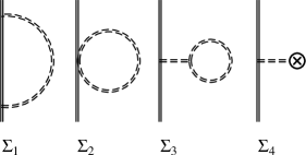
Figure 3: Contributions to the one–loop generating functional ($\Sigma_{1}$, $\Sigma_{2}$, $\Sigma_{3}$) and the tree level mesonic generating functional ($\Sigma_{4}$) at order $\hbar$. The solid (dashed) lines denote the baryon (meson) propagator in the presence of external fields. The circle–cross in $\Sigma_{4}$ denotes the counter terms from ${\cal L}_{M}^{(4)}$. The contributions $\Sigma_{1,2}$ are called irreducible, whereas $\Sigma_{3,4}$ are reducible.

Only if one ensures that the field definitions underlying the meson and the baryon–meson Lagrangian match, the divergences are entirely given by the irreducible self–energy ($\Sigma_{1}$) and the tadpole ($\Sigma_{2}$) graphs. The explicit calculations to extract the divergences from $\Sigma_{1,2}$ are given in [28] for SU(2) to third order, in [33] for SU(3) to third order and in [34] for SU(2) to fourth order employing standard heat kernel techniques. In the baryon sector, this technique is somewhat ackward due to the different treatment of the bosonic and the fermionic propagators. Therefore, in Ref.35 a super–heat–kernel technique inspired from supersymmetry methods was proposed and used in [36] for the chiral pion–nucleon Lagrangian to third order. The so constructed divergences in the generating functional are simple poles in $1/(d-4)$. These can be renormalized by introducing the appropriate local counterterm Lagrangian to that order with corresponding LECs of the form Eq.(10). In that way, one constructs in general a fairly long list of terms, i.e. complete set for the renormalization with off–shell baryons. As long as one is only interested in Greens functions with on–shell baryons, the number of terms can be reduced considerably by making use of the baryon equations of motion. Also, many of these terms involve processes with three or more mesons. Such terms rarely show up in actual calculations. For more details on the procedure, the reader should consult in particular Ref.33.

Consider now renormalization within the relativistic approach based on IR regularization. To leading order, the infrared singular parts coincide with the heavy baryon expansion, in particular the infinite parts of loop integrals are the same. Therefore, the $\beta$–functions for low energy constants which absorb these infinities are identical. However, infrared singular parts of relativistic loop integrals also contain infinite parts which are suppressed by powers of $M_{\pi}/m_{N}$, which hence cannot be absorbed as long as one only introduces counterterms to a finite order: exact renormalization only works up to the order at which one works, higher order divergences have to be removed by hand. Closely related to this problem is the one of the new mass scale $\lambda$ which one has to introduce in the progress of regularization and renormalization. In dimensional regularization and related schemes, loop diagrams depend logarithmically on $\lambda$. This $\log\lambda$ dependence is compensated for by running coupling constants, the running behavior determined by the corresponding $\beta$–functions. In the same way as the contact terms cannot consistently absorb higher order divergences, their $\beta$–functions cannot compensate for scale dependence which is suppressed by powers of $\mu$. In order to avoid this unphysical scale dependence in physical results, the authors of [32] have argued that the nucleon mass $m_{N}$ serves as a “natural” scale in a relativistic baryon CHPT loop calculation and that therefore, one should set $\lambda=m_{N}$ everywhere when using the infrared regularization scheme. This was already suggested in [23] for the framework of a relativistic theory with ordinary dimensional regularization.

3.8 Power counting

To calculate any process to a given order, it is mandatory to have a compact expression for the chiral power counting.[9] [38] Consider first purely mesonic or single–baryon processes. To be precise, I consider the heavy baryon approach, but these rules can be extended to the relativistic treatment based on the IR regularization method. Any amplitude for a given physical process has a certain chiral dimension $D$ which keeps track of the powers of external momenta and meson masses, collectively labelled by the integer $d$. The building blocks to calculate this chiral dimension from a general Feynman diagram in the CHPT loop expansion are (i) $I_{M}$ Goldstone boson (meson) propagators $\sim 1/(\ell^{2}-M^{2})$ (with $M=M_{\pi,K,\eta}$ the meson mass) of dimension $D=-2$, (ii) $I_{B}$ baryon propagators $\sim 1/v\cdot\ell$ (in HBCHPT) with $D=-1$, (iii) $N_{d}^{M}$ mesonic vertices with $d=2,4,6,\ldots$ and (iv) $N_{d}^{MB}$ meson–baryon vertices with $d=1,2,3,\ldots$. Each loop integration introduces four powers of momenta. Putting pieces together, the chiral dimension $D$ of a given amplitude reads

$$D=4L-2I_{M}-I_{B}+\sum_{d}d(\,N_{d}^{M}+N_{d}^{MB}\,)$$ (60)

with $L$ the number of loops. For connected diagrams, one can use the general topological relation

$$L=I_{M}+I_{B}-\sum_{d}(\,N_{d}^{M}+N_{d}^{MB}\,)+1$$ (61)

to eliminate $I_{M}$ :

$$D=2L+2+I_{B}+\sum_{d}(d-2)N_{d}^{M}+\sum_{d}(d-2)N_{d}^{MB}~{}.$$ (62)

Lorentz invariance and chiral symmetry demand $d\geq 2$ for mesonic interactions and thus the term $\sum_{d}(d-2)N_{d}^{M}$ is non–negative. Therefore, in the absence of baryon fields, Eq. (62) simplifies to [9]

$$D=2L+2+\sum_{d}(d-2)N_{d}^{M}\,\geq 2L+2~{}.$$ (63)

To lowest order $p^{2}$, one has to deal with tree diagrams ($L=0$) only. Loops are suppressed by powers of $p^{2L}$. Next, consider processes with a single baryon line running through the diagram (i.e., there is exactly one baryon in the in– and one baryon in the out–state). In this case, the identity

$$\sum_{d}N_{d}^{MB}=I_{B}+1$$ (64)

holds leading to [38]

$$D=2L+1+\sum_{d}(d-2)N_{d}^{M}+\sum_{d}(d-1)N_{d}^{MB}\,\geq 2L+1~{}.$$ (65)

Therefore, tree diagrams start to contribute at order $p$ and one–loop graphs at order $p^{3}$. Let me now consider diagrams with $N_{\gamma}$ external photons. Since gauge fields like the electromagnetic field appear in covariant derivatives, their chiral dimension is obviously $D=1$. One therefore writes the chiral dimension of a general amplitude with $N_{\gamma}$ photons as

$$D=D_{L}+N_{\gamma}~{},$$ (66)

where $D_{L}$ is the degree of homogeneity of the (Feynman) amplitude $A$ as a function of external momenta ($p$) and meson masses ($M$) in the following sense (see also [39]):

$$A(p,M;C_{i}^{r}(\lambda),\lambda/M)=M^{D_{L}}\,A(p/M,1;C_{i}^{r}(\lambda),\lambda/M)~{},$$ (67)

where $\lambda$ is an arbitrary renormalization scale and $C_{i}^{r}(\lambda)$ denote renormalized LECs. From now on, I will suppress the explicit dependence on the renormalization scale and on the LECs. Since the total amplitude is independent of the arbitrary scale $\lambda$, one may in particular choose $\lambda=M$. Note that $A(p,M)$ has also a certain physical dimension (which is of course independent of the number of loops and is therefore in general different from $D_{L}$). The correct physical dimension is ensured by appropriate factors of $F_{\pi}$ and $m$ in the denominators. Finally, consider a process with $E_{n}$ ($E_{n}=4,6,\ldots$) external baryons (nucleons). The corresponding chiral dimension $D_{n}$ follows to be [40]

$$D_{n}=2(L-C)+4-\frac{1}{2}E_{n}+\sum_{i}V_{i}\Delta_{i}\,,\quad\Delta_{i}=d_{i}+\frac{1}{2}n_{i}-2\,\,,$$ (68)

where $C$ is the number of connected pieces and one has $V_{i}$ vertices of type $i$ with $d_{i}$ derivatives and $n_{i}$ baryon fields (these include the mesonic and meson–baryon vertices discussed before). Chiral symmetry demands $\Delta_{i}\geq 0$. As before, loop diagrams are suppressed by $p^{2L}$. Notice, however, that this chiral counting only applies to the irreducible diagrams and not to the full S–matrix since reducible diagrams can lead to IR pinch singularities and need therefore a special treatment (for details, see Refs.40,41).

3.9 Phenomenological interpretation of the LECs

In this section, we will be concerned with the phenomenological interpretation of the values of the dimension two LECs $c_{i}$. For that, guided by experience from the meson sector[42], we use resonance exchange. To introduce these concepts, I briefly discuss the Goldstone boson sector. In the meson sector at next–to-leading order, the effective three flavor Lagrangian ${\cal L}_{M}^{(4)}$ contains ten LECs, called $L_{i}$. These have been determined from data in Ref.11. The actual values of the $L_{i}$ can be understood in terms of resonance exchange.[42] For that, one constructs the most general effective Lagrangian containing besides the Goldstone bosons also resonance degrees of freedom. Integrating out these heavy degrees of freedom from the EFT, one finds that the renormalized $L_{i}^{r}(\mu=M_{\rho})$ are practically saturated by resonance exchange ($S,P,V,A$). In some few cases, tensor mesons can play a role.[43] This is sometimes called chiral duality because part of the excitation spectrum of QCD reveals itself in the values of the LECs. Furthermore, whenever vector and axial resonances can contribute, the $L_{i}^{r}(M_{\rho})$ are completely dominated by $V$ and $A$ exchange, called chiral vector meson dominance (VMD).[44] As an example, consider the finite (and thus scale–independent) LEC $L_{9}$. Its empirical value is $L_{9}=(7.1\pm 0.3)\cdot 10^{-3}$. The well–known $\rho$–meson exchange model for the pion form factor (neglecting the width), $F_{\pi}^{V}(t)=M_{\rho}^{2}/(M_{\rho}^{2}-t)=1+t/M_{\rho}^{2}+{\cal O}(t^{2})$ leads to $L_{9}=F_{\pi}^{2}/(2M_{\rho}^{2})=7.2\cdot 10^{-3}$, by comparing to the small momentum expansion of the pion form factor, $F_{\pi}^{V}(q^{2})=1+\langle r^{2}\rangle_{\pi}\,t/6+{\cal O}(t^{2})$. The resonance exchange result is in good agreement with the empirical value. Even in the symmetry breaking sector related to the quark masses, where only scalar and (non–Goldstone) pseudoscalar mesons can contribute, resonance exchange helps to understand why SU(3) breaking is generally of the order of $25\%$, except for the Goldstone boson masses. Consider now an effective Lagrangian with resonances chirally coupled to the nucleons and pions. One can generate local pion–nucleon operators of higher dimension with given LECs by letting the resonance masses become very large with fixed ratios of coupling constants to masses, symbolically

$$\tilde{{\cal L}}_{\rm eff}[U,M,N,N^{\star}]\to{\cal L}_{\rm eff}[U,N]\,\,,$$ (69)

where $M$ ($N^{\star}$) denotes meson (baryon) resonances. This procedure amounts to decoupling the resonance degrees of freedom from the effective field theory. However, the traces of these frozen particles are encoded in the numerical values of certain LECs. In the case at hand, we can have baryonic and mesonic excitations,

$$c_{i}=\sum_{N^{*}=\Delta,R,\ldots}c_{i}^{N^{*}}+\sum_{M=S,V,\ldots}c_{i}^{M}\,\,\,,$$ (70)

where $R$ denotes the Roper $N^{*}(1440)$ resonance. Consider first scalar ($S$) meson exchange. The SU(2) $S\pi\pi$ interaction can be written as

$${\cal L}_{\pi S}=S\,\Big{[}\bar{c}_{m}\,{\rm Tr}(\chi_{+})+\bar{c}_{d}\,{\rm Tr}(u_{\mu}u^{\mu})\Big{]}\,\,\,.$$ (71)

From this, one easily calculates the s–channel scalar meson contribution to the invariant amplitude $A(s,t,u)$ for elastic $\pi\pi$ scattering,

$$A^{S}(s,t,u) = \frac{4}{F_{\pi}^{4}(M_{S}^{2}-s)}\,[2\bar{c}_{m}M_{\pi}^{2}+\bar{c}_{d}(s-2M_{\pi}^{2})]^{2}$$ (72)

$$\qquad\quad+{16\bar{c}_{m}M_{\pi}^{2}\over 3F_{\pi}^{4}M_{S}^{2}}\Big{[}\bar{c}_{m}M_{\pi}^{2}+\bar{c}_{d}(3s-4M_{\pi}^{2})\big{]}\,\,\,.$$

Comparing to the SU(3) amplitude calculated in,[45] we are able to relate the $\bar{c}_{m,d}$ to the ${c}_{m,d}$ of [42] (setting $M_{S_{1}}=M_{S_{8}}=M_{S}$ and using the large–$N_{c}$ relations $\tilde{c}_{m,d}=c_{m,d}/\sqrt{3}$ to express the singlet couplings in terms of the octet ones), $\bar{c}_{m,d}=c_{m,d}/{\sqrt{2}}$, with $|c_{m}|=42\,$MeV and $|c_{d}|=32\,$MeV.[42] Assuming now that $c_{1}$ is entirely due to scalar exchange, we get $c_{1}^{S}=-(g_{S}\,\bar{c}_{m})/M_{S}^{2}$. Here, $g_{S}$ is the coupling constant of the scalar–isoscalar meson to the nucleons, ${\cal L}_{SN}=-g_{S}\,\bar{N}N\,S$. What this scalar–isoscalar meson is essentially doing is to mock up the strong pionic correlations coupled to nucleons. Such a phenomenon is also observed in the meson sector. The one loop description of the scalar pion form factor fails beyond energies of 400 MeV, well below the typical scale of chiral symmetry breaking, $\Lambda_{\chi}\simeq 1\,$GeV. Higher loop effects are needed to bring the chiral expansion in agreement with the data.[46] Effectively, one can simulate these higher loop effects by introducing a scalar meson with a mass of about 600 MeV. This is exactly the line of reasoning underlying the arguments used here (for a pedagogical discussion on this topic, see [47]). It does, however, not mean that the range of applicability of the effective field theory is bounded by this mass in general. In certain channels with strong pionic correlations one simply has to work harder than in the channels where the pions interact weakly and go beyond the one–loop approximation which works well in most cases. For $c_{1}$ to be completely saturated by scalar exchange, $c_{1}\equiv c_{1}^{S}$, we need $M_{S}/\sqrt{g_{S}}=180\,$MeV. Here we made the assumption that such a scalar has the same couplings to pseudoscalars as the real $a_{0}(980)$ resonance. It is interesting to note that the effective $\sigma$–meson in the Bonn one–boson–exchange potential [48] with $M_{S}=550\,$MeV and $g_{S}^{2}/(4\pi)=7.1$ has $M_{S}/\sqrt{g_{S}}=179\,$MeV. This number is in stunning agreement with the value demanded from scalar meson saturation of the LEC $c_{1}$. With that, the scalar meson contribution to $c_{3}$ is fixed including the sign, since $c_{m}c_{d}>0$, $c_{3}^{S}=-2g_{s}\,\bar{c}_{d}/M_{S}^{2}=2c_{d}\,c_{1}/c_{m}=-1.40\,$GeV^-1. The isovector $\rho$–meson only contributes to $c_{4}$. Taking a universal $\rho$–hadron coupling and using the KSFR relation, $M_{\rho}=\sqrt{2}F_{\pi}g_{\rho}$,[49] we find $c_{4}^{\rho}=\kappa_{\rho}/(4m)=1.63\,$GeV^-1, using $\kappa_{\rho}=6.1\pm 0.4$ from the analysis of the nucleon electromagnetic form factors, the process $\bar{N}N\to\pi\pi$ [50] [51] and the phenomenological one–boson–exchange potential for the NN interaction. I now turn to the baryon excitations. Here, the dominant one is the $\Delta(1232)$. Using the isobar model and the SU(4) coupling constant relation, the $\Delta$ contribution to the various LECs is $c_{2}^{\Delta}=-c_{3}^{\Delta}=2c_{4}^{\Delta}=g_{A}^{2}\,(m_{\Delta}-m)/(2[(m_{\Delta}-m)^{2}-M_{\pi}^{2}])=3.83\,$GeV^-1. There is, however some sizeable uncertainty related to these, see Ref.37. One can deduce the following ranges: $c_{2}^{\Delta}=1.9\ldots 3.8,\,c_{3}^{\Delta}=-3.8\ldots-3.0,\,c_{4}^{\Delta}=1.4\ldots 2.0$ (in GeV^-1). The Roper $N^{*}(1440)$ resonance contributes only marginally, see Ref.37. Putting pieces together, we have for $c_{2}$, $c_{3}$ and $c_{4}$ from resonance exchange

$$c_{2}^{\rm Res} = c_{2}^{\Delta}+c_{2}^{R}=3.83+0.05=3.88\,\,,$$

$$c_{3}^{\rm Res} = c_{3}^{\Delta}+c_{3}^{S}+c_{3}^{R}=-3.83-1.40-0.06=-5.29\,\,,$$

$$c_{4}^{\rm Res} = c_{4}^{\Delta}+c_{4}^{\rho}+c_{4}^{R}=1.92+1.63+0.12=3.67\,\,,$$ (73)

with all numbers given in units of GeV^-1. Comparison with the empirical values listed in table 4 shows that these LECs can be understood from resonance saturation, assuming only that $c_{1}$ is entirely given by scalar meson exchange. The LECs $\stackrel{{\scriptstyle\circ}}{{\kappa}}_{s}=-0.12$ and $\stackrel{{\scriptstyle\circ}}{{\kappa}}_{v}=5.83$ can be estimated from neutral vector meson exchange. For the values from,[50] $\kappa_{\omega}=-0.16\pm 0.01$ and $\kappa_{\rho}=6.1\pm 0.4$, we see that the isoscalar and isovector anomalous magnetic moments in the chiral limit can be well understood from $\omega$ and $\rho^{0}$ meson exchange.

Table 4: Values of the LECs $c_{i}$ in GeV^-1 for $i=1,\ldots,4$. Also given are the central values (cv) and the ranges for the $c_{i}$ from resonance exchange. The ^∗ denotes an input quantity.

$i$	$c_{i}$ Ref.37	$c_{i}$ Ref.20	$c_{i}$ Ref.98	$c_{i}^{\rm Res}\,\,$ cv [ranges]
1	$-0.93\pm 0.10$	$-1.23\pm 0.16$	$-0.81\pm 0.12$	$-0.9^{*}$ [–]
2	$3.34\pm 0.20$	$3.28\pm 0.23$	$8.43\pm 56.9$	$3.9\,\,[2\ldots 4]$
3	$-5.29\pm 0.25$	$5.94\pm 0.09$	$-4.70\pm 1.16$	$-5.3\,\,[-4.5\ldots-5.3]$
4	$3.63\pm 0.10$	$3.47\pm 0.05$	$3.40\pm 0.04$	$3.7\,\,[3.1\ldots 3.7]$

A systematic investigation of dimension three or four LECs is not yet available. It has been found that some dimension three LECs appearing in the chiral description of the nucleon electromagnetic form factors can be understood in terms of vector meson ($\rho,\omega,\phi$) exchanges.

3.10 Isospin violation and extension to virtual photons

Up to now, I have mostly treated pure QCD in the isospin limit. We know, however, that there are essentially two sources of isospin symmetry violation (ISV). First, the quark mass difference $m_{d}-m_{u}$ leads to strong ISV. Second, switching on the electromagnetic (em) interaction, charged particles are surrounded by a photon cloud making them heavier than their neutral partners. An extreme case is the pion, where the strong ISV is suppressed (see below) and the photon cloud is almost entirely responsible for the charged to neutral mass difference. Matters are different for the nucleon. Here, pure electromagnetism would suggest the proton to be heavier than the neutron by 0.8 MeV - at variance with the data. However, the quark mass (strong) contribution can be estimated to be $(m_{n}-m_{p})^{\rm str}=2.1$ MeV. Combining these two numbers, one arrives at the empirical value of $m_{n}-m_{p}=1.3$ MeV. Let me now discuss how these effects arise in CHPT. Consider first the strong interactions. The symmetry breaking part of the QCD Hamiltonian, i.e. the quark mass term, can be decomposed into an isoscalar and an isovector term

$${\cal H}_{\rm QCD}^{\rm sb}=m_{u}\bar{u}u+m_{d}\bar{d}d={1\over 2}(m_{u}+m_{d})(\bar{u}u+\bar{d}d)+{1\over 2}(m_{u}-m_{d})(\bar{u}u-\bar{d}d)\,\,\,.$$ (74)

The quark mass ratios can easily be deduced from the ratios of the (unmixed) Goldstone bosons, in particular, $m_{d}/m_{u}=1.8\pm 0.2$.[52] Therefore, $(m_{d}-m_{u})/(m_{d}+m_{u})\simeq 0.3$ and one could expect large isospin violating effects. However, the light quark masses are only about $5...10$ MeV (at a renormalization scale of 1 GeV) and the relevant scale to compare to is of the order of the proton mass. This effectively suppresses the effect of the sizeable light quark mass difference in most cases, as will be discussed below. We notice that in the corresponding meson EFT, Eq.(33), the isoscalar term appears at leading order while the isovector one is suppressed. This is essentially the reason for the tiny quark mass contribution to the pion mass splitting. On the other hand, in the pion–nucleon system, no symmetry breaking appears at lowest order but at next–to–leading order, the isoscalar and the isovector terms contribute. These are exactly the terms $\sim c_{1}$ and $\sim c_{5}$ in Table 3. In his seminal paper in 1977, Weinberg pointed out that reactions involving nucleons and neutral pions might lead to gross violations of isospin symmetry [53] since the leading terms from the dimension one Lagrangian are suppressed. In particular, he argued that the mass difference of the up and down quarks can produce a 30% effect in the difference of the $\pi^{0}p$ and $\pi^{0}n$ S–wave scattering lengths while these would be equal in case of isospin conservation. This was later reformulated in more modern terminology.[54] To arrive at the abovementioned result, Weinberg considered Born terms and the dimension two symmetry breakers. However, as shown in Ref.55, at this order there are other isospin–conserving terms which make a precise prediction for the individual $\pi^{0}p$ or $\pi^{0}n$ scattering length very difficult. Furthermore, there is no way of directly measuring these processes. On the other hand, there exists a huge body of data for elastic charged pion–nucleon scattering ($\pi^{\pm}p\to\pi^{\pm}p$) and charge exchange reactions ($\pi^{-}p\to\pi^{0}n$). In the framework of some models it has been claimed that the presently available pion–nucleon data basis exhibits strong isospin violation of the order of a few percent.[56] [57] What is, however, uncertain is to what extent the methods used to separate the electromagnetic from the strong ISV effects match. To really pin down isospin breaking due to the light quark mass difference, one needs a machinery that allows to simultaneously treat the electromagnetic and the strong contributions. Here, CHPT comes into the game since one can extend the effective Lagrangian to include virtual photons. To be specific, consider now the photons as dynamical degrees of freedom. To do this in a systematic fashion, one has to extend the power counting. A very natural way to do this is to assign to the electric charge the chiral dimension one, based on the observation that

$$\alpha={e^{2}\over 4\pi}\sim{M_{\pi}^{2}\over(4\pi F_{\pi})^{2}}\sim{1\over 100}\quad.$$ (75)

This is also a matter of consistency. While the neutral pion mass is unaffected by the virtual photons, the charged pions acquire a mass shift of the order $e^{2}$ from the photon cloud. If one would assign the electric charge a chiral dimension zero, then the power counting would be messed up. The extension of the meson Lagrangian is standard, I only give the result here and refer to Refs.42,58,59,60 for all the details. Also, I consider only the two flavor case,

$${\cal L}^{(2)}_{\pi\pi}=-{1\over 4}F_{\mu\nu}F^{\mu\nu}-{\lambda\over 2}(\partial_{\mu}A^{\mu})^{2}+{F_{\pi}^{2}\over 4}\langle\nabla_{\mu}U\nabla^{\mu}U^{\dagger}+\chi U^{\dagger}+\chi^{\dagger}U\rangle+C\langle QUQU^{\dagger}\rangle\,\,,$$ (76)

with $F_{\mu\nu}=\partial_{\mu}A_{\nu}-\partial_{\nu}A_{\mu}$ the photon field strength tensor and $\lambda$ the gauge–fixing parameter (from here on, I use the Lorentz gauge $\lambda=1$). Also,

$$\nabla_{\mu}U=\partial_{\mu}U-i(v_{\mu}+a_{\mu}+QA_{\mu})U+iU(v_{\mu}-a_{\mu}+QA_{\mu})\,\,,$$ (77)

is the generalized pion covariant derivative containing the external vector ($v_{\mu}$) and axial–vector ($a_{\mu}$) sources. It is important to stress that in Refs.42,58,59 $Q$ denotes the quark charge matrix. To make use of the nucleon charge matrix commonly used in the pion–nucleon EFT, one can perform a transformation of the type $Q\to Q+\alpha\,e\,\bf 1$, with $\alpha$ a real parameter. One observes that $d\langle QUQU^{\dagger}\rangle/d\alpha\sim e^{2}\,\bf 1$, i.e. to this order the difference between the two charge matrices can completely be absorbed in an unobservable constant term. The LEC $C$ can be calculated from the neutral to charged pion mass difference via $(\delta M^{2}_{\pi})_{\rm em}=2e^{2}C/F_{\pi}^{2}$. This gives $C=5.9\cdot 10^{-5}\,$GeV⁴. Extending this unique lowest order term in Eq.(76) to SU(3), one can easily derive Dashen’s theorem. To introduce virtual photons in the effective pion–nucleon field theory, consider the nucleon charge matrix $Q=e\,{\rm diag}(1,0)$. Note that contrary to what was done before, the explicit factor $e$ is subsumed in $Q$ so as to organize the power counting along the lines discussed before. For the construction of chiral invariant operators, let me introduce the matrices

$$Q_{\pm}=\frac{1}{2}\,(u\,Q\,u^{\dagger}\pm u^{\dagger}\,Q\,u)\,\,,\quad\widetilde{Q}_{\pm}=Q_{\pm}-{1\over 2}\langle Q_{\pm}\rangle\,\,.$$ (78)

Under chiral SU(2)${}_{L}\times$SU(2)_R symmetry, the $Q_{\pm}$ transform as

$$Q_{\pm}\to h(g,\Phi)\,Q_{\pm}\,h^{-1}(g,\Phi)~{},$$ (79)

in terms of the compensator field introduced in section 3.3. Furthermore, under parity ($P$) and charge conjugation ($C$) transformations, one finds

$$P\,Q_{\pm}\,P^{-1}=\pm\,Q_{\pm}\,\,\,,\quad C\,Q_{\pm}\,C^{-1}=\pm\,Q_{\pm}^{T}\,\,\,.$$ (80)

For physical processes, only quadratic combinations of the charge matrix $Q$ (or, equivalently, of the matrices $Q_{\pm}$) can appear. The following relations are of use,

$$\langle Q_{-}\rangle=\langle Q_{-}\,Q_{+}\rangle=0\,\,,\quad\langle[iD_{\mu},Q_{\pm}]\rangle=0\,\,\,,$$ (81)

together with the SU(2) matrix relations discussed in section 3.3. It is now straightforward to implement the (virtual) photons given in terms of the gauge field $A_{\mu}$ in the effective pion–nucleon Lagrangian. To be specific, I discuss here the heavy baryon approach. Starting from the relativistic theory and decomposing the spinor fields into light (denoted $N$) and heavy components (velocity eigenstates), one can proceed as discussed before. In particular, to lowest order (chiral dimension one),

$${\cal L}_{\pi N}^{(1)}=\bar{N}\,\biggl{(}iv\cdot\bar{D}+g_{A}\,S\cdot\bar{u}\,\biggr{)}\,N\,\,\,,$$ (82)

with

$$\bar{D}_{\mu}=D_{\mu}-i\,Q_{+}\,A_{\mu}\,\,\,,\quad\bar{u}_{\mu}=u_{\mu}-2\,Q_{-}\,A_{\mu}\,\,\,.$$ (83)

At next order (chiral dimension two), we have

$${\cal L}_{\pi N,{\rm em}}^{(2)}=\bar{N}\,F_{\pi}^{2}\,\biggl{\{}{f_{1}}\,\langle Q^{2}_{+}-Q^{2}_{-}\rangle+{f_{2}}\,\widetilde{Q}_{+}\langle Q_{+}\rangle+{f_{3}}\,\langle Q^{2}_{+}+Q^{2}_{-}\rangle\,\biggr{\}}\,N\,\,\,.$$ (84)

I have written down the minimal number allowed by all symmetries. Note that the last term in ${\cal L}_{\pi N,{\rm em}}^{(2)}$ is proportional to $e^{2}\bar{N}N$. This means that it only contributes to the electromagnetic nucleon mass in the chiral limit and is thus not directly observable. However, this implies that in the chiral two–flavor limit ($m_{u}=m_{d}=0$, $m_{s}$ fixed), the proton is heavier than the neutron since it acquires an electromagnetic mass shift. Only in pure QCD ($e^{2}=0$), this chiral limit mass is the same for both particles. The numerical values of the electromagnetic LECs $f_{1}$ and $f_{2}$ will be discussed below. The normalization factor of $F_{\pi}^{2}$ in the electromagnetic pion–nucleon Lagrangian is introduced so that the $f_{i}$ have the same dimension as the strong LECs $c_{i}$. To go beyond tree level, we have to construct the terms of order $p^{3}$ and $p^{4}$ (for a complete one–loop calculation). The third order terms are given in Ref.61 and the fourth order ones in Ref.62, together with a host of applications. The interested reader is referred to these papers. A dimensional analysis of the pertinent electromagnetic LECs is given in appendix C. I briefly return to the neutron–proton mass difference as an instructive example. To order $p^{3}$, it is given by a strong insertion $\sim c_{5}$ and an electromagnetic insertion $\sim f_{2}$,

$$m_{n}-m_{p} = (m_{n}-m_{p})_{\rm str}+(m_{n}-m_{p})_{\rm em}$$ (85)

$$= 4\,c_{5}\,B\,(m_{u}-m_{d})+2\,e^{2}\,F_{\pi}^{2}\,f_{2}+{\cal O}(p^{4})\,\,\,.$$

Note that one–loop corrections only start at order $p^{4}$. This can be traced back to the fact that the photonic self–energy diagram of the proton (on–shell) at order $p^{3}$ vanishes since it is proportional to $\int d^{d}k\,[k^{2}\,v\cdot k]^{-1}$. Such an integral vanishes in dimensional regularization. At chiral dimension three, the electromagnetic LEC $f_{2}$ can therefore be fixed from the electromagnetic proton mass shift, $(m_{n}-m_{p})_{\rm em}=-(0.7\pm 0.3)\,$MeV, i.e. $f_{2}=-(0.45\pm 0.19)\,$GeV^-1. The strong contribution has been used in [37] to fix the LEC $c_{5}=-0.09\pm 0.01\,$GeV^-1. Note that it is known that one–loop graphs with an insertion $\sim m_{d}-m_{u}$ on the internal nucleon line, which in our counting appear at fourth order, can contribute sizeably to the strong neutron-proton mass difference.[63] This calculation can be found in Ref.62. Also, the CHPT framework was used to systematically study ISV in threshold $\pi$N scattering in all physical channels.[64] Some of these results will be discussed in later sections.

3.11 The modern meaning of low–energy theorems

In this section, I will briefly discuss the meaning of the so–called low–energy theorems (LETs) in the context of CHPT, i.e. the generalization of the current algebra LETs (which were called “soft–pion theorems” in section 2.3. I follow essentially Ref.65. Let us first discuss a well–known example of a LET involving the electromagnetic current. Consider the scattering of very soft photons on the proton, i.e., the Compton scattering process $\gamma(k_{1})+p(p_{1})\to\gamma(k_{2})+p(p_{2})$ and denote by $\varepsilon\,(\varepsilon^{\prime})$ the polarization vector of the incoming (outgoing) photon. The transition matrix element $T$ (normalized to $d\sigma/d\Omega=|T|^{2}$) can be expanded in a Taylor series in the small parameter $\delta=|\vec{k_{1}}|/m$. In the forward direction and in a gauge where the polarization vectors have only space components, $T$ takes the form

$$T=a_{0}\,\vec{\varepsilon}\,^{\prime}\cdot\vec{\varepsilon}+i\,a_{1}\,\delta\,\vec{\sigma}\cdot(\vec{\varepsilon}\,^{\prime}\times\vec{\varepsilon}\,)+{\cal O}(\delta^{2})~{}.$$ (86)

The parameter $\delta$ can be made arbitrarily small in the laboratory so that the first two terms in the Taylor expansion (86) dominate. To be precise, the first one proportional to $a_{0}$ gives the low–energy limit for the spin–averaged Compton amplitude, while the second ($\sim a_{1}$) is of pure spin–flip type and can directly be detected in polarized photon proton scattering (to my knowledge, such a test has not yet been performed). The pertinent LETs fix the values of $a_{0}$ and $a_{1}$ in terms of measurable quantities,[66]

$$a_{0}=-\frac{Z^{2}e^{2}}{4\pi m}\,,\quad a_{1}=-\frac{Z^{2}e^{2}\kappa_{p}^{2}}{8\pi m}$$ (87)

with $Z=1$ the charge of the proton. To arrive at Eq. (87), one only makes use of gauge invariance and the fact that the $T$–matrix can be written in terms of a time–ordered product of two conserved vector currents sandwiched between proton states. The derivation proceeds by showing that for small enough photon energies the matrix element is determined by the electromagnetic form factor of the proton at $q^{2}=0$.[66] Similar methods can be applied to other than the electromagnetic currents. In strong interaction physics, a special role is played by the axial–vector currents. The associated symmetries are spontaneously broken giving rise to the Goldstone matrix elements

$$\langle 0|A^{a}_{\mu}(0)|\pi^{b}(p)\rangle=i\delta^{ab}F_{\pi}p_{\mu}~{},$$ (88)

where $a,b$ are isospin indices. In the chiral limit, the massless pions play a similar role as the photon and many LETs have been derived for “soft pions”. In light of the previous discussion on Compton scattering, the most obvious one is Weinberg’s prediction for elastic $\pi p$ scattering.[5] We only need the following translations :

$$\langle p|T\,j_{\mu}^{\rm em}(x)j_{\nu}^{\rm em}(0)|p\rangle\,\,\to\,\,\langle p|T\,A_{\mu}^{\pi^{+}}(x)A_{\nu}^{\pi^{-}}(0)|p\rangle~{},$$ (89)

$$\partial^{\mu}j_{\mu}^{\rm em}=0\,\,\to\,\,\partial^{\mu}A_{\mu}^{\pi^{-}}=0~{}.$$ (90)

In contrast to photons, pions are not massless in the real world. It is therefore interesting to find out how the LETs for soft pions are modified in the presence of non–zero pion masses (due to non–vanishing quark masses). In the old days of current algebra, a lot of emphasis was put on the PCAC relation, consistent with the Goldstone matrix element, Eq.(88),

$$\partial^{\mu}A^{a}_{\mu}=M_{\pi}^{2}F_{\pi}\pi^{a}~{}.$$ (91)

Although the precise meaning of this formalism has long been understood,[67] it does not offer a systematic method to calculate higher orders in the momentum and mass expansion of LETs. The derivation of non–leading terms in the days of current algebra and PCAC was more an art than a science, often involving dangerous procedures like off–shell extrapolations of amplitudes. Current algebra can only provide the leading term in a systematic expansion but can not be used to provide the corrections to these lowest order statements. In the modern language, i.e. the EFT of the Standard Model, these higher order corrections can be calculated unambiguously and one correspondingly defines a low–energy theorem via: L(OW) E(NERGY) T(HEOREM) OF ${\cal O}(p^{n})\equiv$ GENERAL PREDICTION OF CHPT TO ${\cal O}(p^{n})$. By general prediction I mean a strict consequence of the SM depending on some LECs like $F_{\pi},m,g_{A},\kappa_{p},\ldots$, but without any model assumption for these parameters. This definition contains a precise prescription how to obtain higher–order corrections to leading–order LETs. The soft–photon theorems, e.g. for Compton scattering,[66] involve the limit of small photon momenta, with all other momenta remaining fixed. Therefore, they hold to all orders in the non–photonic momenta and masses. In the low–energy expansion of CHPT, on the other hand, the ratios of all small momenta and pseudoscalar meson masses are held fixed. Of course, the soft–photon theorems are also valid in CHPT as in any gauge invariant quantum field theory. To understand this difference of low–energy limits, I will now rederive and extend the LET for spin–averaged nucleon Compton scattering in the framework of HBCHPT.[23] Consider the spin–averaged Compton amplitude in forward direction (in the Coulomb gauge $\varepsilon\cdot v=0$)

$$e^{2}\varepsilon^{\mu}\varepsilon^{\nu}\frac{1}{4}{\rm Tr}\biggl{[}(1+\gamma_{\lambda}v^{\lambda})T_{\mu\nu}(v,k)\biggr{]}=e^{2}\biggl{[}\varepsilon^{2}U(\omega)+(\varepsilon\cdot k)^{2}V(\omega)\biggr{]}$$ (92)

with $\omega=v\cdot k$ ($k$ is the photon momentum) and

$$T_{\mu\nu}(v,k)=\int d^{4}k\,{\rm e}^{ik\cdot x}\,\langle N(v)|Tj^{\rm em}_{\mu}(x)j_{\nu}^{\rm em}(0)|N(v)\rangle~{}.$$ (93)

All dynamical information is contained in the functions $U(\omega)$ and $V(\omega)$. We only consider $U(\omega)$ here and refer to Ref.23 for the calculation of both $U(\omega)$ and $V(\omega)$. In the Thomson limit, only $U(0)$ contributes to the amplitude. In the forward direction, the only quantities with non–zero chiral dimension are $\omega$ and $M_{\pi}$. In order to make this dependence explicit, we write $U(\omega,M_{\pi})$ instead of $U(\omega)$. With $N_{\gamma}=2$ external photons, the degree of homogeneity $D_{L}$ for a given CHPT contribution to $U(\omega,M_{\pi})$ follows from Eq. (65) :

$$D_{L}=2L-1+\sum_{d}(d-2)N_{d}^{M}+\sum_{d}(d-1)N_{d}^{MB}\,\geq-1~{}.$$ (94)

Therefore, the chiral expansion of $U(\omega,M_{\pi})$ takes the following general form :

$$U(\omega,M_{\pi})=\sum_{D_{L}\geq-1}\omega^{D_{L}}f_{D_{L}}(\omega/M_{\pi})~{}.$$ (95)

The following arguments illuminate the difference and the interplay between the soft–photon limit and the low–energy expansion of CHPT. Let us consider first the leading terms in the chiral expansion (95) :

$$U(\omega,M_{\pi})={1\over\omega}f_{-1}(\omega/M_{\pi})+f_{0}(\omega/M_{\pi})+{\cal O}(p)~{}.$$ (96)

Eq. (94) tells us that only tree diagrams can contribute to the first two terms. However, the relevant tree diagrams do not contain pion lines. Consequently, the functions $f_{-1}$, $f_{0}$ cannot depend on $M_{\pi}$ and are therefore constants. Since the soft–photon theorem [66] requires $U(0,M_{\pi})$ to be finite, $f_{-1}$ must actually vanish and the chiral expansion of $U(\omega,M_{\pi})$ can be written as

$$U(\omega,M_{\pi})=f_{0}+\sum_{D_{L}\geq 1}\omega^{D_{L}}f_{D_{L}}(\omega/M_{\pi})~{}.$$ (97)

But the soft–photon theorem yields additional information : since the Compton amplitude is independent of $M_{\pi}$ in the Thomson limit and since there is no term linear in $\omega$ in the spin–averaged amplitude, we find

$$\lim_{\omega\to 0}~{}\omega^{n-1}f_{n}(\omega/M_{\pi})=0\qquad(n\geq 1)$$ (98)

implying in particular that the constant $f_{0}$ describes the Thomson limit :

$$U(0,M_{\pi})=f_{0}~{}.$$ (99)

Let me now verify these results by explicit calculation. In the Coulomb gauge, there is no direct photon–nucleon coupling from the lowest–order effective Lagrangian ${\cal L}_{\pi N}^{(1)}$ since it is proportional to $\varepsilon\cdot v$. Consequently, the corresponding Born diagrams vanish so that indeed $f_{-1}=0$. On the other hand, the heavy mass expansion of the relativistic $\pi N$ Dirac Lagrangian leads to a Feynman insertion of the form:

$$i\frac{e^{2}}{m}\frac{1}{2}(1+\tau_{3})\biggl{[}\varepsilon^{2}-(\varepsilon\cdot v)^{2}\biggr{]}=i\frac{e^{2}Z^{2}}{m}\,\varepsilon^{2}$$ (100)

producing the desired result $f_{0}=Z^{2}/m$, the Thomson limit. At the next order in the chiral expansion, ${\cal O}(p^{3})$ ($D_{L}=1$), the function $f_{1}(\omega/M_{\pi})$ is given by the finite sum of 9 one–loop diagrams.[68] [23] According to Eq. (98), $f_{1}$ vanishes for $\omega\to 0$. The term linear in $\omega/M_{\pi}$ yields the leading contribution to the sum of the electric and magnetic polarizabilities of the nucleon, defined by the second–order Taylor coefficient in the expansion of $U(\omega,M_{\pi})$ in $\omega$ :

$$f_{1}(\omega/M_{\pi})=-{11g_{A}^{2}\omega\over 192\pi F_{\pi}^{2}M_{\pi}}+{\cal O}(\omega^{2})~{}.$$ (101)

The $1/M_{\pi}$ behaviour should not come as a surprise – in the chiral limit the pion cloud becomes long–ranged (instead of being Yukawa–suppressed) so that the polarizabilities explode. This behaviour is specific to the leading contribution of ${\cal O}(p^{3})$. In fact, from the general form (97) one immediately derives that the contribution of ${\cal O}(p^{n})$ ($D_{L}=n-2$) to the polarizabilities is of the form $c_{n}M_{\pi}^{n-4}$ ($n\geq 3$), where $c_{n}$ is a constant that may be zero. One can perform a similar analysis for the amplitude $V(\omega)$ and for the spin–flip amplitude. Next, let us consider the processes $\gamma N\to\pi^{0}N$ $(N=p,n)$ at threshold, i.e., for vanishing three–momentum of the pion in the nucleon rest frame. At threshold, only the electric dipole amplitude $E_{0+}$ survives and the only quantity with non–zero chiral dimension is $M_{\pi}$. In the usual conventions, $E_{0+}$ has physical dimension $-1$ and it can therefore be written as

$$E_{0+}={eg_{A}\over F}~{}A\left({M_{\pi}\over m},{M_{\pi}\over F}\right)~{}.$$ (102)

The dimensionless amplitude $A$ will be expressed as a power series in $M_{\pi}$. The various parts are characterized by the degree of homogeneity (in $M_{\pi}$) $D_{L}$ according to the chiral expansion. Since $N_{\gamma}=1$ in the present case, we obtain from Eq. (65)

$$D_{L}=D-1=2L+\sum_{d}(d-2)N_{d}^{M}+\sum_{d}(d-1)N_{d}^{MB}~{}.$$ (103)

For the LET of ${\cal O}(p^{3})$ in question, only lowest–order mesonic vertices ($d=2$) will appear. Therefore, in this case the general formula for $D_{L}$ takes the simpler form

$$D_{L}=2L+\sum_{d}(d-1)N_{d}^{MB}~{}.$$ (104)

I will not discuss the chiral expansion of $E_{0+}$ step by step, but rather refer to the literature [69] [70] [23] for the actual calculation and for more details to the Comment.[65] Up–to–and–including order $\mu^{2}=(M_{\pi}/m)^{2}$, one has to consider contributions with $D_{L}=0,1$ and $2$. In fact, for neutral pion photoproduction, there is no term with $D_{L}=0$ since the time–honored Kroll–Ruderman contact term [71] where both the pion and the photon emanate from the same vertex, only exists for charged pions. For $D_{L}=2$ there is a one–loop contribution ($L=1$) with leading–order vertices only ($N_{d}^{MB}=0~{}(d>1)$). It is considerably easier to work out the relevant diagrams in HBCHPT [23] than in the original derivation.[69] [70] In fact, at threshold only the so–called triangle diagram (and its crossed partner) survive out of some 60 diagrams. The main reason for the enormous simplification in HBCHPT is that one can choose a gauge without a direct $\gamma NN$ coupling of lowest order and that there is no direct coupling of the produced $\pi^{0}$ to the nucleon at threshold. Notice that the loop contributions are finite and they are identical for proton and neutron. They were omitted in the original version of the LET [72] [73] and in many later rederivations. The full LETs of ${\cal O}(p^{3})$ are given by [69]

$$E_{0+}(\pi^{0}p) = -\displaystyle\frac{eg_{A}}{8\pi F_{\pi}}\biggl{[}\biggr{.}\displaystyle\frac{M_{\pi}}{m}-\displaystyle\frac{M_{\pi}^{2}}{2m^{2}}~{}(3+\kappa_{p})-\displaystyle\frac{M_{\pi}^{2}}{16F_{\pi}^{2}}+\biggl{.}{\cal O}(M_{\pi}^{3})\biggr{]}~{},$$ (105)

$$E_{0+}(\pi^{0}n) = -\displaystyle\frac{eg_{A}}{8\pi F_{\pi}}\biggl{[}\biggr{.}\displaystyle\frac{M_{\pi}^{2}}{2m^{2}}~{}\kappa_{n}-\displaystyle\frac{M_{\pi}^{2}}{16F_{\pi}^{2}}+\biggl{.}{\cal O}(M_{\pi}^{3})\biggr{]}~{}.$$ (106)

We note that the electric dipole amplitude for neutral pion production vanishes in the chiral limit. By now, even the terms of order $M_{\pi}^{3}$ have been worked out, see Ref.[74] The derivation of LETs sketched above is based on a well–defined quantum field theory where each step can be checked explicitly. Nevertheless, the corrected LETs have been questioned by several authors. A detailed discussions of the various assumptions like e.g. analyticity in the pion mass, which do not hold in QCD, can be found in Ref.65. Even better, by now the data support the CHPT predictions, see section 4.7. Consequently, a LET to a certain order as defined here is always strict but might not always be useful (in case of large higher order corrections).

3.12 Inclusion of resonances

This section departs a bit from the main line of reasoning performed so far. Up to now, any QCD state of higher mass (nucleon or meson resonances) appeared only implicitly, in the values of certain LECs. In addition, there is a decoupling theorem,[75] which states that in the chiral limit all S–matrix elements and transition currents to leading order are given in terms of the Goldstone bosons and the ground state baryon octet. Nevertheless, under certain circumstances one has to extend the effective field theory to include some of these resonances explicitly. In particular, when going to higher energies, the usefulness of the chiral expansion is limited by the appearance of the nucleon (or meson) resonances, the most prominent and important of these being the $\Delta(1232)$ with spin and isospin 3/2. Its implications for hadronic and nuclear physics are well established. Consequently, one would like to have a consistent and systematic framework to include this important degree of freedom in baryon chiral perturbation theory, as first stressed by Jenkins and Manohar [76] and only recently formalized by Hemmert, Holstein and Kambor [77] (see also [78] for a general discussion of including the delta). This is possible because one can count the nucleon–delta mass splitting as an additional small parameter. Doing that, one arrives at the so–called small scale expansion. It has already been established that most of the low–energy constants appearing in the effective chiral pion–nucleon Lagrangian are saturated by the delta and thus the resummation of such terms underlying the small scale expansion (SSE) lets one expect a better convergence as compared to the chiral expansion. In addition, the radius of convergence is clearly enlarged when the delta is included as an explicit degree of freedom. This of course increases the complexity of the approach since the pertinent effective Lagrangian contains more structures consistent with all symmetries. Here, I will briefly discuss the structure of the effective Lagrangian underlying the SSE. All this is found in much more detail in the work of Hemmert et al. [77] and I refer the interested reader to that paper to fill in the details omitted here. The explicit inclusion of the delta into an effective pion–nucleon field theory is motivated by the fact that in certain observables this resonance plays a prominent role already at low energies. The reason for this is twofold. First, the delta–nucleon mass splitting is small,

$$\Delta\equiv m_{\Delta}-m_{N}=294~{}{\rm MeV}\simeq 3F_{\pi}~{}$$ (107)

or stated differently, $\Delta={\cal O}(M_{\pi})$. However, in the chiral limit of vanishing quark masses, neither $\Delta$ nor $F_{\pi}$ vanish. Therefore, such an extended EFT does not have the same chiral limit as QCD, as it is well–known since long.[75] Second, the delta couples very strongly to the $\pi N\gamma$ system, e.g. the strong $\Delta N\gamma$ M1 transition plays a prominent role in charged pion photoproduction or nucleon Compton scattering. One can set up a consistent power counting by using the well–known heavy baryon techniques [22, 23] and by treating the mass splitting $\Delta$ as an additional small parameter besides the external momenta and quark (meson) masses. Therefore, any matrix element or transition current has a low energy expansion of the form

$${\cal M}=\varepsilon^{n}\,{\cal M}_{1}+\varepsilon^{n+1}\,{\cal M}_{2}+\varepsilon^{n+2}\,{\cal M}_{3}+{\cal O}(\varepsilon^{n+3})~{},$$ (108)

where the power $n$ depends on the process under consideration (for example in case of elastic pion–nucleon scattering, $n$ equals one) and $\varepsilon$ collects the three different small parameters,

$$\varepsilon\in\left\{{p\over\Lambda_{\chi}},{M_{\pi}\over\Lambda_{\chi}},{\Delta\over\Lambda_{\chi}}\right\}~{},$$ (109)

with $\Lambda_{\chi}\simeq 1\,$GeV the scale of chiral symmetry breaking. This power counting scheme is often called $\varepsilon$– or small scale expansion (SSE). As it is common in heavy baryon approaches, the expansion in the inverse of the heavy mass and with respect to the chiral symmetry breaking scale are treated simultaneously (because $m_{N}\sim m_{\Delta}\sim\Lambda_{\chi}$). The inclusion of the delta is more complicated because as a spin–3/2 field, one has to eliminate not only the “small” spin–3/2 component but also the four intrinsic (“off–shell”) spin–1/2 components. The technology to do that is spelled out in.[77] The resulting effective Lagrangian has the following low–energy expansion

$${\cal L}_{\rm eff}={\cal L}^{(1)}+{\cal L}^{(2)}+{\cal L}^{(3)}+\ldots$$ (110)

where each of the terms ${\cal L}^{(n)}$ decomposes into a pure nucleon ($\pi N$), a nucleon–delta ($\pi N\Delta$) and a pure delta part ($\pi\Delta$),

$${\cal L}^{(n)}={\cal L}^{(n)}_{\pi N}+{\cal L}^{(n)}_{\pi N\Delta}+{\cal L}^{(n)}_{\pi\Delta}~{},\quad n=1,2,3,\ldots~{}.$$ (111)

I will not discuss these terms in detail but only make some general remarks. First, while the terms with nucleon fields only have the same structure as in the pion–nucleon EFT, the presence of the explicit delta modifies of course the numerical values of most LECs. The $N\Delta$ terms are to be understood symmetrically and the pure delta part is mostly needed inside loop integrals. The coupling of external fields is done by standard methods. So far, only some reactions have been investigated systematically in this framework, these are threshold pion photoproduction,[79] Compton scattering,[80, 81] electroweak nucleon and nucleon–delta transition form factors [82, 83] or pion–nucleon scattering.[84] Some of the pertinent results will be discussed below.

It is also well established that in many reations vector mesons play a prominent role. A formal study of chiral Lagrangians involving baryons, Goldstone bosons and spin–1 fields is given in.[85] At present, there is no generalization of CHPT which fully includes the effects of vector mesons as intermediate states to arbitrary loop orders. As the masses of the vector mesons do not vanish in the chiral limit, they introduce a new mass scale which, when appearing inside loop integrals, potentially spoils chiral power counting in a similar manner as the nucleon mass in a “naive” relativistic baryon CHPT approach. In analogy to the heavy fermion theories, “heavy meson effective theory” has been used to investigate vector meson properties like masses and decay constants when coupling these to the Goldstone bosons in a chirally invariant fashion (see [86] or for some special processes [87]). This approach does not work with the heavy particle number not conserved as in processes with these resonances being virtual intermediate states. However, these difficulties do not arise as long as there is no loop integration over intermediate vector meson momenta. Such special cases will be discussed below.

4 Two flavors: The structure of the nucleon

4.1 Two–point functions I: The nucleon mass

It is instructive to consider the chiral expansion of the nucleon mass in heavy baryon CHPT. Here, I will be concerned with the chiral SU(2) limit, i.e. $m_{u}=m_{d}=0$ and $m_{s}$ fixed at its physical value. That means that possible effects due to strangeness admixture into the nucleon wave function are subsumed in the value of the nucleon mass in the chiral limit, which is denoted by $\stackrel{{\scriptstyle\circ}}{{m}}$. One expects that the corrections at $n^{\rm th}$ order are given by $c_{n}M_{\pi}^{n}/\Lambda_{\chi}^{n-1}$, with $c_{n}$ of order one. To fourth order in small momenta, the chiral expansion of the nucleon mass reads:[27, 88]

$$m = \stackrel{{\scriptstyle\circ}}{{m}}-4M^{2}c_{1}-\frac{3g_{A}^{2}M^{3}}{32\pi F^{2}}$$ (112)

$$\quad-M^{4}(16\bar{e}_{38}+2\bar{e}_{115}+\frac{1}{2}\bar{e}_{116})+\frac{3M^{4}c_{2}}{128\pi^{2}F^{2}}-\frac{3g_{A}^{2}M^{4}}{64\pi^{2}mF^{2}}~{}.$$

The LECs $c_{1,2}$ can in principle be determined from the analysis of pion–nucleon scattering discussed in section 4.5. Note that while the term $\sim\bar{e}_{38}$ is nothing but a quark mass renormalization of the operator $\sim c_{1}$, the LECs $\bar{e}_{115,116}$ cannot be determined from pion–nucleon scattering. Setting the fourth order LECs to zero, one finds that the chiral expansion of the nucleon mass is well–behaved and follows the scaling arguments given above

$$\delta m^{(4)}=(72.5-15.1+0.4-0.4)~{}{\rm MeV}~{},$$ (113)

using the LECs as determined in.[37] The fifth order contribution has been determined in Ref.89, they find that all loop contributions cancel and that one is simply left with a $1/m$ correction to the third order piece, which is numerically tiny. This is a good starting point for further investigations of $n$–point functions in HBCHPT. The effects due to virtual photons have also been worked out to fourth order.[62] At third order, one only has an effect due to the pion mass difference, which is a 7% correction to the strong result given in Eq.(112). The fourth order correction depends on the em LEC $f_{1}$ and other known LECs.[62] Setting $f_{1}=\pm 1/(4\pi)$ as expected from dimensional analysis (see app. C), the numerical value of the em fourth order mass shift is tiny, for the proton one finds $\delta m^{(4,\rm em)}_{p}=-0.10\ldots-0.01\,$MeV and for the neutron $\delta m^{(4,\rm em)}_{n}=-0.06\ldots+0.03\,$MeV. This is completely negligible and comparable to the strong fourth order mass shift. This shows that the effects of virtual photons can be calculated with their precise values depending on the electromagnetic LECs. Most of these can at present only be estimated using dimensional analysis (as discussed before).

4.2 Three–point functions I: Scalar form factor and sigma term

Pion–nucleon scattering data allow to extract information on the size of the pion–nucleon $\sigma$–term, $\sigma(0)$, which measures the explicit chiral symmetry breaking in QCD due to the up– and down–quark masses. A venerable (current algebra) low–energy theorem due to Brown, Pardee and Peccei [90] relates $\sigma(0)$ to the isoscalar $\pi$N scattering amplitude (with the pseudovector Born term subtracted) via

$$F_{\pi}^{2}\,\bar{D}^{+}(0,2M_{\pi}^{2})-\sigma(2M_{\pi}^{2})=F_{\pi}^{2}\,\bar{D}^{+}(0,2M_{\pi}^{2})-\Delta\sigma-\sigma(0)=\Delta_{R}=M_{\pi}^{4}\,C_{R}~{},$$ (114)

with $\Delta\sigma=\sigma(2M_{\pi}^{2})-\sigma(0)$. The crucial statement of the low–energy theorem is that the remainder $\Delta_{R}$ grows quadratically with the light quark mass, because $C_{R}$ is a quark mass independent constant. At the Cheng–Dashen point $\nu=0,\,s=m^{2},\,t=2M_{\pi}^{2}$,[91]

$$\bar{D}^{+}(0,2M_{\pi}^{2})=A^{+}(m^{2},2M_{\pi}^{2})-{g_{\pi N}^{2}\over m}\,\,\,,$$ (115)

in terms of the standard isospin even $\pi$N scattering amplitude $A^{+}(\nu,t)$ and the last term is due to the subtraction of the pseudovector tree amplitude. Furthermore, the nucleon scalar form factor $\sigma(t)$ is given by the matrix element

$$\langle N(p^{\prime})|\hat{m}(\bar{u}u+\bar{d}d)|N(p)\rangle=\bar{u}(p^{\prime})u(p)\,\sigma(t)~{},\quad t=(p-p^{\prime})^{2}\,\,\,,$$ (116)

with $\hat{m}=(m_{u}+m_{d})/2$ the average light quark mass. Although the Cheng–Dashen point is not in the physical region of the $\pi$N scattering process, it lies well within the Lehmann ellipse and thus $\bar{D}^{+}(0,2M_{\pi}^{2})$ can be obtained by analytic continuation, i.e. using dispersion relations. Employing the only available coherent phase shift analyses, KA80 [92] and KA85,[93] leads to $F_{\pi}^{2}\,\bar{D}^{+}(0,2M_{\pi}^{2})=60\,(62)\,$MeV.[94] For a discussion of the uncertainties (typically $\pm 8$ MeV) and previous determinations, I refer to.[94] There is also on–going debate about the size of this quantity and I refer to Ref.95 for the various opinions. The leading non–analytic contribution to the scalar form factor difference, $\Delta\sigma$, is $3g_{\pi N}^{2}M_{\pi}^{3}/(64\pi m^{2})$ and gives about 8 MeV.[96] [21] A detailed dispersive analysis [94], with $\pi\pi$ and $\pi$N information consistent with chiral symmetry, yields $\Delta\sigma=15.2\pm 0.4\,$MeV. The remainder $\Delta_{R}$ is not fixed by chiral symmetry. It has to be known, however, in order to extract information on the $\sigma$–term, i.e. $\sigma(0)$, and from it the strangeness content of the proton, i.e. the matrix element $\langle p|\,\bar{s}s\,|p\rangle$, via the so–called strangeness fraction

$$y=\frac{2\langle p|\,\bar{s}s\,|p\rangle}{\langle p|\,\bar{u}u+\bar{d}d\,|p\rangle}~{}.$$ (117)

The strangeness fraction can also be related to the baryon mass spectrum via $\sigma=\hat{m}\,(m_{\Xi}-m_{\Sigma}-2m_{N})/(m_{s}-\hat{m})/(1-y)+{\cal O}(m_{q}^{3/2})$. The remainder $\Delta_{R}$ has been evaluated to order $q^{4}$ in HBCHPT in.[97] It was proven that $C_{R}$ has $no$ chiral logarithm and thus it is finite in the chiral limit. To this order, only local contact terms contribute to the remainder. The result based on the complete $q^{4}$ CHPT calculation with the low energy constants of the pertinent counterterms saturated via resonance exchange is

$$\Delta_{R}\approx 2\,{\rm MeV}\,\,\,,$$ (118)

which should be considered an upper bound. As conjectured in Ref.94 the remainder $\Delta_{R}$ indeed does not play any role in the extraction of the $\sigma$–term from the $\pi$N data considering the present status of accuracy of these data in the threshold region. Thus, the analysis of Ref.94 leads to

$$\sigma(0)\simeq 45\,{\rm MeV}~{},\quad\Delta\sigma\simeq 15\,{\rm MeV}~{},\quad y\simeq 0.2~{}.$$ (119)

This value for the sigma term has been confirmed using a different method in.[98] Of course, the KA80 and KA85 phase shift analyses are based on some data which are considered inconsistent right now. All modern data are included in the partial wave analysis of the GW/VPI group and reevaluations of the sigma term based on that should be available in the near future. However, it is mandatory that the same precise machinery, i.e. combining dispersion relations with chiral symmetry constraints, is used to obtain reliable results. This point is particularly stressed in Ref.98. In the case of isospin violation, one has of course to differentiate between the proton and the neutron $\sigma$–terms, as detailed in Ref.61. There it was shown that the third order effects can shift the proton $\sigma$–term by about 8% and have a smaller influence on the shift to the Cheng–Dashen point. The isospin violating corrections to this shift to fourth order were evaluated in Ref.62 and were found to be very small. However, it was also shown that there is an isospin conserving electromagnetic contribution to the shift which can be as large as $\pm 2\,$MeV, which is a substantial electromagnetic effect. What is still missing is a complete reanalysis of the LET [90] in the presence of strong and electromagnetic isospin violation.

4.3 Three–point functions II: Electromagnetic form factors

The structure of the nucleon as probed by virtual photons is parameterized in terms of four form factors (here, $N$ is the fully relativistic spin–1/2 field),

$$\langle N(p^{\prime})\,|\,{\cal J}_{\mu}\,|\,N(p)\rangle=e\,\bar{u}(p^{\prime})\,\biggl{\{}\gamma_{\mu}F_{1}^{N}(t)+\frac{i\sigma_{\mu\nu}k^{\nu}}{2m}F_{2}^{N}(t)\biggr{\}}\,u(p)\,,\quad N=p,n\,,$$ (120)

with $t=k_{\mu}k^{\mu}=(p^{\prime}-p)^{2}$ the invariant momentum transfer squared and ${\cal J}_{\mu}$ the em current related to the photon field. In electron scattering, $t$ is negative and it is thus convenient to define the positive quantity $Q^{2}=-t>0$. $F_{1}$ and $F_{2}$ are called the Pauli and the Dirac form factor (ff), respectively, with the normalizations $F_{1}^{p}(0)=1$, $F_{1}^{n}(0)=0$, $F_{2}^{p}(0)=\kappa_{p}$ and $F_{2}^{n}(0)=\kappa_{n}$. Also used are the electric and magnetic Sachs ffs,

$$G_{E}=F_{1}-\tau F_{2}\,,\quad G_{M}=F_{1}+F_{2}\,,\quad\tau=Q^{2}/4m^{2}\,.$$ (121)

In the Breit–frame, $G_{E}$ and $G_{M}$ are nothing but the Fourier–transforms of the charge and the magnetization distribution, respectively. These are the natural quantities for the heavy nucleon scheme.[23] There exists already a large body of data for the proton and also for the neutron. In the latter case, one has to perform some model–dependent extractions to go from the deuteron or ³He to the neutron. There are also data in the time–like region from the reactions $e^{+}e^{-}\to p\bar{p},n\bar{n}$ and from annihilation $p\bar{p}\to e^{+}e^{-}$, for $t\geq 4m_{N}^{2}$. A largely model–independent analysis of this body of data is based on dispersion theory using an unsubtracted dispersion relation for $F(t)$ (which is a generic symbol for any one of the four ff’s),

$$F(t)=\frac{1}{\pi}\int_{t_{0}}^{\infty}\,dt^{\prime}\,\frac{{\rm Im}\,F(t)}{t^{\prime}-t}\,\,,$$ (122)

with $t_{0}$ the two (three) pion threshold for the isovector (isoscalar) ffs. Im $F(t)$ is called the spectral function. It is advantageous to work in the isospin basis, $F_{i}^{s,v}=F_{i}^{p}\pm F_{i}^{n}$, since the photon has an isoscalar ($I=s$) and an isovector ($I=v$) component. These spectral functions are the natural meeting ground for theory and experiment, like e.g. the partial wave amplitudes in $\pi N$ scattering. In general, the spectral functions can be thought of as a superposition of vector meson poles and some continua, related to n-particle thresholds, like e.g. $2\pi$, $3\pi$, $K\bar{K}$, $N\bar{N}$ and so on. For example, in the Vector Meson Dominance (VMD) picture one simply retains a set of poles. It is important to realize that there are some powerful constraints which the spectral functions have to obey. Consider the spectral functions just above threshold. Here, unitarity plays a central role. As pointed out by Frazer and Fulco [99] long time ago, extended unitarity leads to a drastic enhancement of the isovector spectral functions on the left wing of the $\rho$ resonance. This is due to a logarithmic singularity on the second Riemann sheet at the anomalous threshold $t_{c}=4M_{\pi}^{2}-(M_{\pi}^{4}/m^{2})=3.98M_{\pi}^{2}$, very close to the normal threshold $t_{0}=4M_{\pi}^{2}$. Leaving out this contribution from the two–pion cut leads to a gross underestimation of the isovector charge and magnetic radii. This very fundamental constraint is often overlooked. In the framework of chiral pertubation theory, this enhancement is also present at the one–loop level as first shown in Ref.21. It is also correctly given when using the method of infrared regularization,[100] but distorted in the strict heavy baryon approach as detailed in Ref.101. The question whether a similar phenomenon appears in the isoscalar spectral function has been answered in HBCHPT.[101] For that, one has to consider certain two–loop graphs. Although the analysis of Landau equations reveals a branch point on the second Riemann sheet close to the threshold at $t_{0}=9M_{\pi}^{2}$, the three–body phase factors suppress its influence in the physical region. Consequently, the spectral functions rise smoothly up to the $\omega$ pole and the common practice of simply retaining vector meson poles at low $t$ in the isoscalar channel is justified. The ffs have been worked out to third order in Refs.23,82 and to fourth order in[102] as shown by the dashed lines for the electric ffs in Fig.4.

Figure 4: Electric form factor of the neutron. The dashed lines refer to the HBCHPT and the solid ones to the IR regularized relativistic calculation. The order is indicated by the number on each line. The dot–dashed line is the dispersion theoretical analysis of Ref.50. The data are from MAMI, BATES and NIKHEF involving polarized ³He targets or polarization transfer on deuterium.

At third order, one has two electric counterterms which can be fixed from fitting the proton and the neutron charge radius and two counterterms which are fixed from the magnetic moments of the proton and the neutron. To that order, the momentum dependence of the magnetic ffs is free of counterterms. At fourth order, one has two additional magnetic counterterms, which allow to fix the proton and neutron magnetic radius. Still, only for momentum transfer $Q^{2}<0.2\,$GeV² one gets a decent description for the large ffs ($G_{E}^{p}$, $G_{M}^{p}$ and $G_{M}^{n}$) whereas the relative magnitude of the fourth order corrections to the neutron electric ff becomes large at even smaller $Q^{2}$. As can be seen from the figure, the use of IR regularization (which has no additional counterterms) clearly improves the situation for $G_{E}^{n}$, not only is the prediction much closer to the data up to $Q^{2}\simeq 0.4\,$GeV² but also the difference between the third and fourth order is sizeably reduced up to higher $Q^{2}$. However, the predictions for the large (dipole–like) ffs are not very much affected. The coupling of vector mesons in a chirally invariant way allows to fix this problems without any new parameters (these can be taken from existing determinations based on dispersion theory [50, 103]), as shown in Fig.5 for the magnetic ff of the proton. Very similar results are found for the electric proton and the magnetic neutron form factors. On the other hand, the good prediction for the neutron electric form factor is not destroyed (because the vector meson contributions largely cancel in this case). To be more precise, one can formulate an effective chiral Lagrangian including spin–1 fields,[85] which then allows to substitute the local contact terms by explicit vector meson dynamics and a remainder, which is refitted as in the case of the pure pion–nucleon Lagrangian and turns out to be small for most but not all operators (chiral VMD). For details, the reader should consult Ref.100. Clearly, the pion cloud plays an important role in a precise description of these fundamental nucleon structure observables but needs to be supplemented by vector meson dynamics.

Figure 5: Magnetic form factor of the proton. The dashed lines refer to the IR regularized relativistic calculation. The solid lines are obtained by adding in vector mesons in a chirally invariant way and readjusting the LECs to the radius. The chiral order is indicated by the number on each line. The dot–dashed line is the dispersion theoretical analysis of Ref.50.

Within the framework of the SSE, discussed in section 3.12, one can also calculate form factors related to the delta or to nucleon–delta transitions. In Ref.83, the isovector $N\Delta$–transition was calculated to third order in the SSE. The transition matrix element is parametrized in terms of three form factors $G_{1,2,3}(Q^{2})$. To that order, one has only two non–vanishing and finite loop diagrams and all counterterms are momentum–independent. That means that the $Q^{2}$–dependence of the transition ffs is predicted in a parameter–free way and thus is a good testing ground for chiral dynamics. Since the intermediate $\pi N$ state can go on mass–shell, these ffs are complex, even at $Q^{2}=0$. That is not accounted for in most models. These ffs can be mapped uniquely onto the multipole amplitudes $M_{1}(Q^{2})$, $E_{2}(Q^{2})$ and $C_{2}(Q^{2})$, measurable in pion photo/electroproduction. Consequently, the $Q^{2}$–dependence of the so–called EMR $E_{2}/M_{1}$ and of the so–called CMR $C_{2}/M_{1}$ can be predicted. In Fig.6 the momentum dependence of the CMR is shown (for a similar plot for the EMR, see [83]). The various lines refer to the multipole analysis of the Mainz, RPI and VPI groups, which are used to pin down the LECs at $Q^{2}=0$. A more detailed discussion of these topics can be found in.[83] It will be important to confront the recent measurements from ELSA and BATES with these predictions.

Figure 6: The ratio $C_{2}/M_{1}$ versus $Q^{2}$. The solid, dashed and dot–dashed line refer to input from the Mainz, RPI and VPI multipole analysis, in order.

4.4 Three–point functions III: Axial form factors

The structure of the nucleon as probed by charged axial currents is encoded in two form factors – the axial and the induced pseudoscalar ones, denoted by $G_{A}$ and $G_{P}$, respectively. To be specific, consider the matrix element of the isovector axial quark current, $A_{\mu}^{a}=\bar{q}\gamma_{\mu}\gamma_{5}(\tau^{a}/2)q$, between nucleon states,

$$\langle N(p^{\prime})|A_{\mu}^{a}|N(p)\rangle=\bar{u}(p^{\prime})\left[G_{A}(t)\gamma_{\mu}+\frac{G_{P}(t)}{2m_{N}}(p^{\prime}-p)_{\mu}\right]\gamma_{5}{\tau^{a}\over 2}u(p)~{},$$ (123)

where $t=(p^{\prime}-p)^{2}$ is the invariant momentum transfer squared. In the axial matrix element one has assumed the absence of second class currents (in agreement with the data). While $G_{A}(t)$ can be extracted from (anti)neutrino–proton scattering or charged pion electroproduction data, $G_{P}(t)$ is harder to pin down (from muon capture or pion electroproduction) and in fact constitutes the least known nucleon form factor. Consider first the axial form factor. To one loop accuracy, it is given by $G_{A}(t)=g_{A}(1+t\langle r_{A}^{2}\rangle/6)$, with the axial radius containing one LEC. Still, CHPT has been used to make an interesting prediction, namely that this radius as extracted from charged pion electroproduction is different from the one obtained by analyzing neutrino–proton scattering data by a computable and unique loop correction,[105]

$$\Delta\langle r_{A}^{2}\rangle=\frac{3}{64F_{\pi}^{2}}\left(1-\frac{12}{\pi^{2}}\right)=-0.046\,{\rm fm}^{2}~{},$$ (124)

subject to small fourth order corrections.[24] Translated into a dipole mass via $\langle r_{A}^{2}\rangle=12/M_{A}^{2}$, this amounts to a shift in the axial mass by $\Delta M_{A}=0.056\,$GeV. This prediction has recently been verified at MAMI,[106] they find $\Delta M_{A}=(0.043\pm 0.026)\,$GeV (for more details, I refer to that paper). Consider now $G_{P}(t)$. Based on the chiral Ward identities of QCD, a very precise prediction for the induced pseudoscalar form factor was given in [104] (see that paper for a brief discussion on the history of that quantity)

$$G_{P}(t) = \frac{4m_{N}g_{\pi N}F_{\pi}}{M_{\pi}^{2}-t}-\frac{2}{3}g_{A}m_{N}^{2}r_{A}^{2}\;,$$ (125)

which leads to a very accurate prediction for the induced pseudoscalar coupling constant, $g_{P}=(M_{\mu}/2m)G_{P}(t=-0.88M_{\mu}^{2})=8.44\pm 0.23$, with $M_{\mu}$ the muon mass. The theoretical uncertainty is almost entirely due to our poor knowledge of the pion–nucleon coupling constant, $g_{\pi N}=13.05\ldots 13.40$. The first term on the right hand side of Eq.(125) is nothing but the pion pole (current algebra) result. This prediction agrees with the much less precise experimental determination extracted from ordinary muon capture (OMC).[107] It has, however, been challenged by the recent TRIUMF result deduced from radiative muon capture (which is based on a Born term model [110] to extract $g_{P}$ from the photon spectrum), $g_{P}^{\rm RMC}=12.35\pm 0.88\pm 0.38=1.46\,g_{P}^{\rm CHPT}$. This has spurred some sizeable theoretical activity, see e.g. Refs.111,112,113. Although this puzzle is not yet resolved, the most promising ideas towards its solution are spelled out in.[114] Much like in the case of the pion–nucleon sigma term, a sum of various small effects seems to make up this sizeable discrepancy. In any case, the Born model analysis underlying the extraction is certainly very doubtful. Next, let me discuss the momentum dependence of $G_{P}$. In Fig.7 the difference between the usual pion-pole parameterization for $G_{P}(t)$ and the full chiral structure of the form factor is displayed. The data shown in that figure are from one pion electroproduction experiment [108] and one data point is from OMC.[107] In this kinematical regime the structure proportional to $r_{A}^{2}$ produces the biggest effect and a new dedicated experiment should be able to verify it. In fact, at the Mainz Microtron MAMI-B an experiment has been proposed to measure the axial and the induced pseudoscalar form factors by means of charged pion electroproduction at low momentum transfer.[115]

Figure 7: The “world data” for the induced pseudoscalar form factor $G_{P}(t)$. Dashed curve: Pion–pole prediction. Solid curve: Full chiral prediction. The pion electroproduction data (crosses) are from Ref.108. Also shown is the OMC result from Ref.107 (open square).

4.5 Four–point functions I: Pion–nucleon scattering

In the following, we consider elastic $\pi N$ scattering. In the center-of-mass system (cms) the amplitude for the process $\pi^{a}(q_{1})+N(p_{1})\to\pi^{b}(q_{2})+N(p_{2})$ takes the following form (in the isospin basis):

$$T^{ba}_{\pi N} = \biggl{(}\frac{E+m}{2m}\biggr{)}\,\biggl{\{}\delta^{ba}\Big{[}g^{+}(\omega,t)+i\vec{\sigma}\cdot(\vec{q}_{2}\times\vec{q}_{1}\,)\,h^{+}(\omega,t)\Big{]}$$ (126)

$$\qquad\quad+i\,\epsilon^{bac}\tau^{c}\Big{[}g^{-}(\omega,t)+i\vec{\sigma}\cdot(\vec{q}_{2}\times\vec{q}_{1}\,)\,h^{-}(\omega,t)\Big{]}\biggr{\}}~{},$$

with $\omega=v\cdot q_{1}=v\cdot q_{2}$ the pion cms energy, $t=(q_{1}-q_{2})^{2}$ the invariant momentum transfer squared, $E_{1}=E_{2}\equiv E=(\vec{q\,}^{2}+m^{2})^{1/2}$ the nucleon energy and $\vec{q\,}_{1}^{2}=\vec{q\,}_{2}^{2}\equiv\vec{q\,}^{2}=((s-M^{2}-m^{2})^{2}-4m^{2}M^{2})/(4s)$. Furthermore, $g^{\pm}(\omega,t)$ refers to the isoscalar/isovector non–spin–flip amplitude and $h^{\pm}(\omega,t)$ to the isoscalar/isovector spin–flip amplitude. This form is most suitable for the HBCHPT calculation since it is already defined in a two–component framework. These amplitudes can then be projected onto partial waves by standard methods and at threshold lead to the pertinent scattering lengths $(a^{\pm}_{l\pm}$) and effective ranges $(b^{\pm}_{l\pm}$), with $l$ the orbital angular momentum and the total angular momentum $j=l\pm 1/2$. Pion–nucleon scattering has played a very important role in establishing chiral symmetry in hadron physics as discussed before. The first corrections to Weinberg’s CA prediction for the S–wave scattering lengths were considered in Ref.55 including third order loop graphs and contact interactions. The LECs were estimated by resonance saturation. In Ref.116 it was further shown that the dominant correction to the Weinberg–Tomozawa result for the isovector S–wave scattering length is a pure loop effect. More systematic third order studies were performed in Refs.20,37,117. Finally, in Ref.88 the complete fourth–order one–loop results were presented. At this order, one has 14 LECs, which were determined by a fit to the existing S– and P–wave phases from various partial wave analyses for pion momenta between 50 and 100 MeV. This allows to make predictions for the threshold parameters and the phase shifts at higher energies. A typical result is shown in Fig.8, where the dotted lines give the first order result and the dot-dashed, dashed and solid lines refer to the best fit at second (4 LECs), third (9 LECs) and fourth (14 LECs) order. Clearly, one observes convergence as long as the pion momenta stay below 200 MeV. Of particular interest are the predictions for the the S–wave scattering lengths $a^{\pm}_{0+}$. We find $-1.0\leq a^{+}_{0+}\leq 0.6$ and $8.3\leq a^{-}_{0+}\leq 9.3$ in units of $10^{-2}/M_{\pi}$. The uncertainties are mostly due to the input, i.e. to the various phase shift analyses in the physical region, and not to the theory. It is instructive to study the convergence, using e.g. the KA85 phases as input, one finds

$$\begin{array}[]{c|rrrr}&{\cal O}(p)&{\cal O}(p^{2})&{\cal O}(p^{3})&{\cal O}(p^{4})\\ \hline\cr a^{+}_{0+}&0.0&0.46&-1.00&-0.96\\ a^{-}_{0+}&7.90&7.90&9.05&9.03\\ \end{array}$$ (127)

where ${\cal O}(p^{n})$ means that all terms up–to–and–including order $n$ are included. Note that the fourth order correction for the isoscalar scattering length is not large and that the small difference between the third and fourth order results for the isovector one is due to the readjustment of a LEC. Translated into the physical channels, we have

$$\begin{array}[]{lll}a_{\pi^{-}p\to\pi^{0}n}=&-0.131\ldots-0.117\,M_{\pi}^{-1}&[(-0.128\pm 0.006)\,M_{\pi}^{-1}]~{},\\ a_{\pi^{-}p\to\pi^{-}p}=&$\,\,\,\,\,$0.073\ldots$\,\,\,\,\,$0.093\,M_{\pi}^{-1}&[(0.0883\pm 0.0008)\,M_{\pi}^{-1}]~{},\\ \end{array}$$ (128)

where the experimental numbers (in the brackets) are taken from Ref.119. It is worth emphasizing that the theoretical prediction is of similar precision as the experimental one.

Figure 8: HBCHPT description of the S– and P–wave phase shifts as described in the text. The data are from Ref.118.

Higher threshold parameters can be predicted without any free parameters, these are collected in table 5. The agreement with the determination from dispersion theory is mostly satisfactory. However, the HBCHPT representation of the amplitude is not precise enough to also give stable predictions for the so–called subthreshold parameters when the LECs are determined in the physical region. On the other hand, using dispersion theory one can determine the LECs from a fit within the interior of the Mandelstam triangle.[98] In particular, the LEC $c_{1}$, which governs the size of the sigma term, comes out very different to the determinations from fitting the phase shifts. It is hoped that the approach based on the IR regularization will give better results in this context.

Table 5: D– and F–wave threshold parameters predicted by CHPT[37]. The order of the prediction is also given together with the ”experimental values”, which come from the Karlsruhe–Helsinki dispersive analysis.[120]

Obs.	CHPT	Order	Exp. value	Units
$a^{+}_{2+}$	$-1.83$	$p^{3}$	$-1.8\pm 0.3$	$10^{-3}\,M_{\pi}^{-5}$
$a^{+}_{2-}$	$2.38$	$p^{3}$	$2.20\pm 0.33$	$10^{-3}\,M_{\pi}^{-5}$
$a^{-}_{2+}$	$3.21$	$p^{3}$	$3.20\pm 0.13$	$10^{-3}\,M_{\pi}^{-5}$
$a^{-}_{2-}$	$-0.21$	$p^{3}$	$0.10\pm 0.15$	$10^{-3}\,M_{\pi}^{-5}$
$a^{+}_{3+}$	$0.29$	$p^{3}$	$0.43$	$10^{-3}\,M_{\pi}^{-7}$
$a^{+}_{3-}$	$0.06$	$p^{3}$	$0.15\pm 0.12$	$10^{-3}\,M_{\pi}^{-7}$
$a^{-}_{3+}$	$-0.20$	$p^{3}$	$-0.25\pm 0.02$	$10^{-3}\,M_{\pi}^{-7}$
$a^{-}_{3-}$	$0.06$	$p^{3}$	$0.10\pm 0.02$	$10^{-3}\,M_{\pi}^{-7}$

4.6 Four–point functions II: Real and virtual Compton scattering

As discussed before, the low–energy Compton scattering amplitude can be decomposed into a spin–independent, called $f_{1}$, and a spin–dependent part, denoted by $f_{2}$. In forward direction, the T–matrix takes the form

$$T(\gamma N\to\gamma N)=f_{1}(\omega)\,{\vec{\epsilon}\,^{\prime}}{}^{*}\cdot\vec{\epsilon}+f_{2}(\omega)\,\omega\,i\vec{\sigma}\cdot({\vec{\epsilon}\,^{\prime}}{}^{*}\times\vec{\epsilon})$$ (129)

in terms of the photon polarization four–vectors ($\vec{\epsilon},{\vec{\epsilon}\,^{\prime}}$), the photon energy $\omega$ and the nucleon spin matrix $\vec{\sigma}$. In the spin–independent case, the nucleon structure is encoded in the so–called electromagnetic polarizabilities, denoted $\bar{\alpha}$ (electric) and $\bar{\beta}$ (magnetic),

$$f_{1}(\omega)={e^{2}Z^{2}\over m}+(\bar{\alpha}+\bar{\beta})\omega^{2}+{\cal O}(\omega^{4})~{},$$ (130)

with the first term being the Thomsom amplitude discussed before. These polarizabilities have been measured over the years at Illinois, Mainz, Moscow, Oak Ridge and Saskatoon. Calculations have been performed to fourth order with some LECs determined from data and others from resonance saturation. The leading third order one–loop result, which is free of any LEC and solely due to finite loop graphs, has been given a decade ago,[121, 23]

$$\bar{\alpha}_{p}=\bar{\alpha}_{n}=10\bar{\beta}_{p}=10\bar{\beta}_{n}={5e^{2}g_{A}^{2}\over 384\pi^{2}F_{\pi}^{2}M_{\pi}}=12.5\cdot 10^{-4}~{}{\rm fm}^{3}~{},$$ (131)

which describes the trend of the data, namely that the electric polarizability is considerably larger than the magnetic one and also that the sum of both spin–independent polarizabilities is approximately the same for the proton and the neutron. This latter statement is based on the so–called Baldin sum rule, which relates the sum of the electric and magnetic polarizabilities to an integral over the total photoabsorption cross section. Older and more recent evaluations[122, 123, 124] give $(\bar{\alpha}+\bar{\beta})_{p}=(14.2\pm 0.5),(13.69\pm 0.14),(14.0\pm 0.5)\cdot 10^{-4}$ fm³ and $(\bar{\alpha}+\bar{\beta})_{n}=(15.8\pm 0.5),(14.40\pm 0.66),(15.2\pm 0.5)\cdot 10^{-4}$ fm³. The third order investigation has then be supplemented by a fourth order calculation, mostly triggered by the suspicion that the result for the magnetic polarizabilities, which are believed to receive a large order $p^{4}$ contribution from the $\Delta$ resonance, is accidental. A summary of the predictions as compared to the data for the proton reads

$$\begin{array}[]{crr}\bar{\alpha}_{p}=&(10.5\pm 2.0)\cdot 10^{-4}\,{\rm fm}^{3}&[(12.1\pm 0.8\pm 0.5)\cdot 10^{-4}\,{\rm fm}^{3}]~{},\\ \bar{\beta}_{p}=&(3.5\pm 3.6)\cdot 10^{-4}\,{\rm fm}^{3}&[(2.1\mp 0.8\mp 0.5)\cdot 10^{-4}\,{\rm fm}^{3}]~{},\\ \end{array}$$ (132)

The experimental numbers in the square brackets are taken from Ref.125. While in case of the proton a consistent picture is emerging,[126] the published empirical values deduced from scattering slow neutrons on heavy atoms have recently been put into question.[127] Furthermore, recent measurements of elastic and of quasi–free Compton scattering from the deuteron at SAL lead to contradictory results for the neutron polarizabilities.[128, 129] Therefore, I refrain here from comparing the chiral predictions to the data. This experimental problem remains to be sorted out. The most promising result is the almost complete cancellation of a negative non–analytic pion loop contribution with the large positive contribution of tree level $\Delta$–exchange in case of the proton magnetic polarizability.[126] This is the first time that a consistent picture of the para– and diamagnetic contributions to $\bar{\beta}_{p}$ has been found and it underlines the importance of chiral, i.e. pion loop, physics in understanding the nucleon structure as revealed in Compton scattering.

Furthermore, there exist chiral predictions for the four spin–dependent polarizabilities, denoted $\gamma_{1,2,3,4}$. As of today, no direct measurements exist but some indirect information based on multipole analysis points towards the important role of the $\Delta(1232)$ as an active degree of freedom to understand some of these quantities. In table 6, the present status of the theoretical precdictions compared with the indirect determinations is given. For a cleaner separation of the effects of third and fourth order, the isosaclar and isovector contributions are given. These are related to the ones of the proton and neutron via $\gamma_{i}^{(p)}=\gamma_{i}^{(s)}+\gamma_{i}^{(v)}$, and $\gamma_{i}^{(n)}=\gamma_{i}^{(s)}-\gamma_{i}^{(v)}$. Note, however, that with the advent of polarized targets and new sources with a high flux of polarized photons, the case of polarized Compton scattering off the proton, $\vec{\gamma}\,\vec{p}\rightarrow\gamma p$, has come close to experimental feasibility. It thus remains an active field to further sharpen these theoretical predictions.[130] Also, as can be seen from table 6, there is large $\Delta$ contribution to the spin–polarizabilities $\gamma_{2,4}$. In the conventional power counting such effects only start to appear via counterterms at fifth order. Thus, in such a case the explicit inclusion of the delta is mandatory. Other calculations of the spin polarizabilities can be found in Refs.131,132.

Table 6: Predictions for the spin-polarizabilities in HBChPT in comparison with the dispersion analyses of Refs.133,134,135 and the ${\cal O}(\epsilon^{3})$ results of the small scale expansion [81] (SSE1). All results are given in the units of $10^{-4}\;{\rm fm}^{4}$.

	${\cal O}(p^{3})$	${\cal O}(p^{4})$	Sum	Mainz1	Mainz2	BGLMN	SSE1
$\gamma_{1}^{(s)}$	$+4.6$	$-2.1$	$+2.5$	$+5.6$	$+5.7$	$+4.7$	$+4.4$
$\gamma_{2}^{(s)}$	$+2.3$	$-0.6$	$+1.7$	$-1.0$	$-0.7$	$-0.9$	$-0.4$
$\gamma_{3}^{(s)}$	$+1.1$	$-0.5$	$+0.6$	$-0.6$	$-0.5$	$-0.2$	$+1.0$
$\gamma_{4}^{(s)}$	$-1.1$	$+1.5$	$+0.4$	$+3.4$	$+3.4$	$+3.3$	$+1.4$
$\gamma_{1}^{(v)}$	-	$-1.3$	$-1.3$	$-0.5$	$-1.3$	$-1.6$	-
$\gamma_{2}^{(v)}$	-	$-0.2$	$-0.2$	$-0.2$	$+0.0$	$+0.1$	-
$\gamma_{3}^{(v)}$	-	$+0.1$	$+0.1$	$-0.0$	$+0.5$	$+0.5$	-
$\gamma_{4}^{(v)}$	-	$+0.0$	$+0.0$	$+0.0$	$-0.5$	$-0.6$	-

Virtual Compton scattering (VCS), in which one of the photons has a non–vanishing virtuality, offers additional information about the nucleon structure. The VCS amplitude can be parameterized in terms of six so–called generalized polarizabilities (for a precise definition I refer to Refs.136,137). In unpolarized electron scattering, one can extract two of these generalized polarizabilities from the cross section after properly subtracting the dominant contributions from the Bethe–Heitler process and nucleon form factors. That this is indeed possible was recently demonstrated at MAMI.[138] Unpolarized VCS was measured at $Q^{2}=0.33\,$GeV². As shown in Fig. 9, the measured structure functions compare favorably with the third order heavy baryon prediction of Ref.139. Clearly, the fourth order corrections have to be calculated to solidify this result, eventually also using the previously described relativistic formalism. Since this field is very active both theoretically and experimentally (MIT-Bates, MAMI, Jefferson Lab), we are looking forward to many interesting developments.

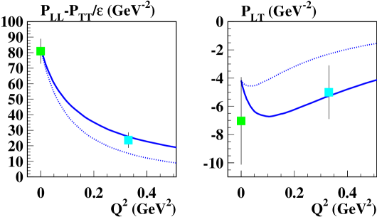
Figure 9: The influence of the generalized polarizabilities on unpolarized VCS (solid line) in comparison to the MAMI measurement at $Q^{2}=0.33\,$GeV². Dashed line: Structure functions obtained by switching off the spin–dependent polarizabilities.

4.7 Four–point functions III: Pion photo– and electroproduction

Charged pion photoproduction at threshold is well described in terms of the Kroll–Ruderman contact term, which is non–vanishing in the chiral limit. All chiral corrections including the third order in the pion mass have been calculated.[140] The chiral series is quickly converging and the theoretical error on the CHPT predictions is rather small, see table 7. The LECs have been determined from resonance exchange. Notice that these uncertainties do not account for the variations in the pion–nucleon coupling constant. The available threshold data are quite old, with the exception of the recent TRIUMF experiment on the inverse reaction $\pi^{-}p\to\gamma n$ and the SAL measurement for $\gamma p\to\pi^{+}n$. While the overall agreement is quite good for the $\pi^{+}n$ channel, in the $\pi^{-}p$ channel the CHPT prediction is on the large side of the data. Clearly, we need more precise data to draw a final conclusion. It is, however, remarkable to have predictions with an error of only 2% .

Table 7: Predictions and data for the charged pion electric dipole amplitudes in $10^{-3}/M_{\pi^{+}}$.

	${\cal O}(p^{4})$	Experiment
$E_{0+}^{\rm thr}(\pi^{+}n)$	$28.2\pm 0.6$	$27.9\pm 0.5$ [141], $28.8\pm 0.7$ [142], $27.6\pm 0.6$ [143]
$E_{0+}^{\rm thr}(\pi^{-}p)$	$-32.7\pm 0.6$	$-31.4\pm 1.3$ [141], $-32.2\pm 1.2$ [144], $-31.5\pm 0.8$ [145]

The threshold production of neutral pions is much more subtle since the corresponding electric dipole amplitudes vanish in the chiral limit. Space does not allow to tell the tale of the experimental and theoretical developments concerning the electric dipole amplitude for neutral pion production off protons, for details see.[146] Even so the convergence for this particular observable is slow, a CHPT calculation to order $p^{4}$ does allow to understand the energy dependence of $E_{0+}$ in the threshold region once three LECs are fitted to the total and differential cross section data,[147] see the left panel of Fig.10. The threshold value agrees with the data, see table 8. Even more interesting is the case of the neutron. Here, CHPT predicts a sizeably larger $E_{0+}$ than for the proton (in magnitude). The CHPT predictions for $E_{0+}(\pi^{0}p,\pi^{0}n)$ in the threshold region clearly exhibit the unitary cusp due to the opening of the secondary threshold, $\gamma p\to\pi^{+}n\to\pi^{0}p$ and $\gamma n\to\pi^{-}p\to\pi^{0}n$, respectively. Note, however, that while $E_{0+}(\pi^{0}p)$ is almost vanishing after the secondary threshold, the neutron electric dipole amplitude is sizeable ($-0.4$ compared to $2.8$ in units of $10^{-3}/M_{\pi^{+}}$). The question arises how to measure the neutron amplitude? The natural neutron target is the deuteron. The corresponding electric dipole $E_{d}$ amplitude has been calculated to order $p^{4}$ in Ref.148. It was shown that the next–to–leading order three–body corrections and the possible four–fermion contact terms do not induce any new unknown LEC and one therefore can calculate $E_{d}$ in parameter–free manner. Furthermore, the leading order three–body terms are dominant, but one finds a good convergence for these corrections and also a sizeable sensitivity to the elementary neutron amplitude. Note also that neutral pion production off deuterium has recently been measured at SAL. The CHPT prediction in comaprison to the data for the reduced cross section of coherent neutral pion production off deuterium is shown in the right panel of Fig.10.

Figure 10: Left panel: CHPT prediction (solid line) for the electric dipole amplitude in $\gamma p\to\pi^{0}p$ in comparison to the data from MAMI and SAL. The dashed line gives the prediction of the incorrect ancient LET discussed in section 3.11. Right panel: Reduced total cross section for $\gamma d\to\pi^{0}d$. The data from SAL are depicted by the boxes, the CHPT threshold prediction is the star on the the dotted line (indicating the threshold photon energy).

Still, there is more interesting physics in these channels. Quite in contrast to what was believed for a long time, there exist a set of LETs for the slopes of the P–waves $P_{1,2}=3E_{1+}\pm M_{1+}\mp M_{1-}$ at threshold, for example

$$\frac{1}{|\vec{q}\,|}P_{1,{\rm thr}}^{\pi^{0}p}=\frac{eg_{\pi N}}{8\pi m^{2}}\left\{1+\kappa_{p}+\mu\left[-1-\frac{\kappa_{p}}{2}+\frac{g_{\pi N}^{2}}{48\pi}(10-3\pi)\right]+{\cal O}(\mu^{2})\right\}\,\,.$$ (133)

Numerically, this translates into

$$\frac{1}{|\vec{q}\,|}P_{1,{\rm thr}}^{\pi^{0}p}=0.512\,(1-0.062)\,{\rm GeV}^{-2}=0.480\,{\rm GeV}^{-2}\,\,,$$ (134)

which is given in table 8 in units which are more used in the literature. The agreement with the data is stunning. A theoretical uncertainty on this order $p^{3}$ calculation can only be given when the next order has been calculated. That calculation is underway. Soon, there will also be an experimental value for $P_{2}$ at threshold once the MAMI data on $\vec{\gamma}p\to\pi^{0}p$ have been analyzed.

Table 8: Predictions and data for neutral pion S– and P–wave multipoles. Units are $10^{-3}/M_{\pi^{+}}$ and $|q||k|10^{-3}/M_{\pi^{+}}^{3}$ for the S–and P–waves, respectively.

	CHPT	Order	Experiment
$E_{0+}^{\rm thr}(\pi^{0}p)$	$-1.16$ [147]	$p^{4}$	$-1.31\pm 0.08$ [149], $-1.32\pm 0.05$ [150]
$P_{1}^{\rm thr}(\pi^{0}p)$	$10.3$ [140]	$p^{3}$	$10.02\pm 0.15$ [149], $10.26\pm 0.1$ [150]
$E_{0+}^{\rm thr}(\pi^{0}d)$	$-1.8\pm 0.2$ [148]	$p^{4}$	$-1.7\pm 0.2$ [151], $-1.5\pm 0.1$ [152]

Producing the pion with virtual photons offers further insight since one can extract the longitudinal S–wave multipole $L_{0+}$ and also novel P–wave multipoles. Data have been taken at NIKHEF [153] [154] and MAMI [155] for photon virtuality of $k^{2}=-0.1$ GeV². In fact, it has been argued previously that such photon four–momenta are already too large for CHPT tests since the loop corrections are large.[156] However, these calculations were performed in relativistic baryon CHPT and thus it was necessary to redo them in the heavy fermion formalism. This was done in.[157] The abovementioned data for differential cross sections were used to determine the three novel S–wave LECs. I should mention that one of the operators used is of dimension five, i.e. one order higher than the calculation was done. This can not be circumvented since it was shown that the two S–waves are overconstrained by a LET valid up to order $p^{4}$. The resulting S–wave cross section $a_{0}=|E_{0+}|^{2}+\varepsilon_{L}\,|L_{0+}|^{2}$ shown in Fig. 11 is in fair agreement with the data. Note also that it is dominated completely by the $L_{0+}$ multipole (upper dot-dashed line) since $E_{0+}$ passes through zero at $k^{2}\simeq-0.04$ GeV². However, in agreement with the older (and less precise) calculations, the one loop corrections are large so one should compare at lower photon virtualities. In Ref.157, many predictions for $k^{2}\simeq-0.05$ GeV² are given. At MAMI, data have been taken in this range of $k^{2}$ and we are looking forward to their analysis, in particular it will be interesting to nail down the zero–crossing of the electric dipole amplitude and to test the novel electroproduction P–wave LETs.[158] I remark that the preliminary analysis of thes data at lower virtuality seems to indicate some inconsistency with the chiral prediction if one uses the data at $k^{2}=-0.1$ GeV² to pin down the LECs.

Figure 11: The S–wave cross section $a_{0}$ compared to the data for various photon polrizations. The upper (lower) dash–dotted line gives the contribution of the longitudinal (electric) dipole amplitude to $a_{0}$ for $\epsilon=0.79$ (solid line).

4.8 Five–point functions I: Electromagnetic two–pion production

Electromagnetic production of two pions off a nucleon can be used to study the excitation of certain nucleon resonances, in particular the $\Delta(1232)$, the Roper $N^{*}(1440)$ or the $D_{15}(1520)$. However, close to threshold one observes an interesting effect due to the chiral pion loops of QCD. To be specific, consider the reaction $\gamma p\to\pi\pi N$, where the two pions in the final state can both be charged, both neutral or one charged and one neutral. To leading order in the chiral expansion, the production of two neutral pions is strictly suppressed. However, at next–to–leading order, due to finite chiral loops the production cross section for final states with two neutral pions is considerably enhanced.[159] Also, in a small window above threshold, the potentially large contribution from double–delta excitation is strongly suppressed, leaving a window in which one can detect much more neutrals than expected. This prediction was further sharpened in Ref.160, where all fourth order corrections including the excitation of the Roper and its successive decay into two neutral pions here considered. The predicted near threshold cross section is

$$\sigma_{\rm tot}(E_{\gamma})\leq 0.91~{}{\rm nb}~{}\biggl{(}{E_{\gamma}-E_{\gamma}^{\rm thr}\over 10~{}{\rm MeV}}\biggr{)}^{2}~{},$$ (135)

with $E_{\gamma}^{\rm thr}=308.8\,$MeV. This prediction can only be applied for the first 30 MeV above threshold. A recent measurement by the TAPS collaboration [161] has shown that such an enhancement of the the 2$\pi^{0}$ production indeed happens, see Fig.12, proving once again the importance of pion loop effects, which can lead to rather unexpected predictions and results.

Figure 12: Total cross section for the process $\gamma p\to\pi^{0}\pi^{0}p$ as measured by the TAPS collaboration at MAMI.[161] The solid line is the fourth order HBCHPT prediction. I am grateful to the TAPS collaboration for providing me with this figure.

4.9 Five–point functions I: $\pi N\to\pi\pi N$

Single pion production off nucleons has been at the center of numerous experimental and theoretical investigations since many years. One of the original motivations of these works was the observation that the elusive pion–pion threshold S–wave interaction could be deduced from the pion–pole graph contribution. A whole series of precision experiments at PSI, TRIUMF, CERN and other laboratories has been performed over the last decade and there is still on–going activity. On the theoretical side, chiral perturbation theory has been used to consider these processes. Beringer considered the reaction $\pi N\to\pi\pi N$ to lowest order in chiral perturbation theory.[162] Low–energy theorems for the threshold amplitudes $D_{1}$ and $D_{2}$ were derived in,[163]

$$D_{1}=\frac{g_{A}}{8F_{\pi}^{3}}\left(1+\frac{7M_{\pi}}{2m}\right)+{\cal O}(M_{\pi}^{2})=2.4\,\,{\rm fm}^{3}\,\,,$$ (136)

$$D_{2}=-\frac{g_{A}}{8F_{\pi}^{3}}\left(3+\frac{17M_{\pi}}{2m}\right)+{\cal O}(M_{\pi}^{2})=-6.8\,\,{\rm fm}^{3}\,\,.$$ (137)

These are free of unknown parameters and not sensitive to the $\pi\pi$–interaction beyond tree level. A direct comparison with the threshold data for the channel $\pi^{+}p\to\pi^{+}\pi^{+}n$, which is only sensitive to $D_{1}$, leads to a very satisfactory description whereas in case of the process $\pi^{-}p\to\pi^{0}\pi^{0}n$, which is only sensitive to $D_{2}$, sizeable deviations are found for the total cross sections near threshold. These were originally attributed to the strong pionic final–state interactions in the $I_{\pi\pi}=0$ channel. However, this conjecture turned out to be incorrect when a complete higher order calculation of the threshold amplitudes $D_{1,2}$ was performed.[164] In that paper, the relation between the threshold amplitudes $D_{1}$ and $D_{2}$ for the reaction $\pi N\to\pi\pi N$ and the $\pi\pi$ S–wave scattering lengths $a_{0}^{0}$ and $a_{0}^{2}$ in the framework of HBCHPT to second order in the pion mass was worked out. Notice that the pion loop and pionic counterterm corrections only start contributing to the $\pi\pi N$ threshold amplitudes at second order. One of these counterterms, proportional to the low–energy constant $\ell_{3}$, eventually allows to measure the scalar quark condensate, i.e. the strength of the spontaneous chiral symmetry breaking in QCD. However, at that order, the largest contributions to $D_{1,2}$ stem indeed from insertions of the dimension two chiral pion–nucleon Lagrangian, which is characterized by the LECs $c_{i}$. In particular this is the case for the amplitude $D_{2}$. To be specific, consider the threshold amplitudes $D_{1,2}$ calculated from the relativistic Born graphs (with lowest order vertices) and the relativistic $c_{i}$–terms expanded to second order in the pion mass. This gives $D_{1}^{{\rm Born}}+D_{1}^{c_{i}}=(2.33+0.24\pm 0.10)\,{\rm fm}^{3}=(2.57\pm 0.10)\,{\rm fm}^{3}\,$, $D_{2}^{{\rm Born}}+D_{2}^{c_{i}}=(-6.61-2.85\pm 0.06)\,{\rm fm}^{3}=(-9.46\pm 0.06)\,{\rm fm}^{3}\,$, which are within 14% and 5% off the empirical values, $D_{1}^{\exp}=(2.26\pm 0.10)\,{\rm fm}^{3}$ and $D_{2}^{\exp}=(-9.05\pm 0.36)\,{\rm fm}^{3}\,$, respectively. It appears therefore natural to extend the same calculation above threshold and to compare to the large body of data for the various reaction channels that exist.[165] It was already shown by Beringer [162] that taking into account only the relativistic Born terms does indeed not suffice to describe the total cross section data for incoming pion energies up to 400 MeV in most channels. Such a failure can be expected from the threshold expansion of $D_{2}$, where the Born terms only amount to 73% of the empirical value. We therefore expect that the inclusion of the dimension two operators, which clearly improves the prediction for $D_{2}$ at threshold, will lead to a better description of the above threshold data. In particular, it will tell to which extent loop effects are necessary (and thus testing the sensitivity to the pion–pion interaction beyond tree level) and to which extent one has to incorporate explicit resonance degrees of freedom like the Roper and the $\Delta$–isobar as well as heavier mesons ($\sigma,\rho,\omega$) as dynamical degrees of freedom (as it is done in many models, see e.g. [166] [167]). Since the LECs $c_{i}$ have previously been determined, all results to this order[165] are based on a truly parameter–free calculation. One finds that (a) for pion energies up to $T_{\pi}=250\,$MeV, in all but one case the inclusion of the contribution $\sim c_{i}$ clearly improves the description of the total cross sections. Up to $T_{\pi}=400\,$MeV, the trend of the data can be described although some discrepancies particularly towards the higher energies persist, and (b) double differential cross sections for $\pi^{-}p\to\pi^{+}\pi^{-}n$ at incident pion energies below $T_{\pi}=250\,$MeV are well described. These findings were further strengthened and extended by the results of a complete third order HBCHPT calculation presented in.[168] It was shown that the effect of unitarity corrections (pion loops) is indeed very small, justifying the use of tree level models, and that the available threshold data are not precise enough to pin down the LEC $\ell_{3}$. The predictions for the total cross sections of all five physical channels are shown in Fig.13 in comparison to the available data for incoming pion momenta up to 400 MeV. Despite the large momentum transfers involved, the chiral description works fairly well, in particular in the $\pi^{-}p\to\pi^{+}\pi^{-}n$ channel. On the other hand, for the two reactions $\pi^{+}p\to\pi^{+}\pi^{+}n$ and $\pi^{-}p\to\pi^{0}\pi^{-}p$ the chiral prediction overshoots the data for energies larger than 300 MeV. For further results and discussion, see.[168]

Figure 13: Predictions for the total cross sections up to incoming pion kinetic energy of $T_{\pi}=400\,$MeV (solid lines). Fitted in each channel are the data below $T_{\pi}=250\,$MeV. The dashed and dotted lines refer to the second and first order contributions, respectively.

5 Three flavors: Hyperons, cascades and the nucleon revisited

5.1 General remarks

Chiral baryon dynamics with strange quarks is a much less developed field than the two–flavor (pion–nucleon) case discussed so far, for two reasons. First, the strange quark mass is sizeably larger so that it is not a priori clear that it can be treated perturbatively. Second, the appearance of close to or even subthreshold resonances (the most prominent example being the $\Lambda(1405)$) in some channels requires some non–perturbative resummation. Ultimately, one is after a marriage of such techniques with chiral symmetry constraints. Although some pionering work has been done, see e.g. the papers and reviews,[169, 170] I will focus here on the results obtained in“plain” chiral perturbation theory.

5.2 Two–point functions I: From baryon to quark masses

The scalar sector of baryon CHPT is particularly interesting since it is sensitive to scalar–isoscalar operators and thus directly to the symmetry breaking of QCD. This is most obvious for the pion– and kaon–nucleon $\sigma$–terms, which measure the strength of the scalar quark condensates $\bar{q}q$ in the proton. Here, $q$ is a generic symbol for any one of the light quarks $u$, $d$ and $s$. Furthermore, the quark mass expansion of the baryon masses allows to give bounds on the ratios of the light quark masses. The quark mass expansion of the octet baryon masses takes the form

$$m=\,\,\stackrel{{\scriptstyle\circ}}{{m}}+\sum_{q}\,B_{q}\,m_{q}+\sum_{q}\,C_{q}\,m_{q}^{3/2}+\sum_{q}\,D_{q}\,m_{q}^{2}+\ldots$$ (138)

modulo logs. Here, $\stackrel{{\scriptstyle\circ}}{{m}}$ is the octet mass in the chiral limit of vanishing quark masses and the coefficients $B_{q},C_{q},D_{q}$ are state–dependent. Furthermore, they include contributions proportional to some LECs which appear beyond leading order in the effective Lagrangian. If one retains only the terms linear in the quark masses, one obtains the Gell-Mann–Okubo relation $m_{\Sigma}+3m_{\Lambda}=2(m_{N}+m_{\Xi})$ (which is fulfilled within 0.6 percent in nature) for the octet and the equal spacing rule for the decuplet, $m_{\Omega}-m_{\Xi^{*}}=m_{\Xi^{*}}-m_{\Sigma^{*}}=m_{\Sigma^{*}}-m_{\Delta}$ (experimentally, one has 142:145:153 MeV). At third order, the leading non-analytic terms $\sim m_{q}^{3/2}$ are generated from finite loop graphs. In contrast, the order $p^{4}$ loops are no longer finite, thus requiring renormalization. A complete fourth order calculation (in the isospin limit $m_{u}=m_{d}$) was presented in.[171] There are 10 LECs related to symmetry breaking, which can be estimated from a generalized resonance saturation hypothesis, i.e. from loop graphs with intermediate baryon excitations. The analytic pieces of such diagrams can be mapped onto higher order symmetry breaking terms, for details see Ref.171. Within this scheme, one finds for the octet baryon mass in the chiral limit $\stackrel{{\scriptstyle\circ}}{{m}}=(770\pm 110)\,{\rm MeV}$. The quark mass expansion of the baryon masses, in the notation of Eq.(138), reads

$$m_{N}=\,\stackrel{{\scriptstyle\circ}}{{m}}\,(1+0.34-0.35+0.24\,)\,\,,$$

$$m_{\Lambda}=\,\stackrel{{\scriptstyle\circ}}{{m}}\,(1+0.69-0.77+0.54\,)\,\,,$$

$$m_{\Sigma}=\,\stackrel{{\scriptstyle\circ}}{{m}}\,(1+0.81-0.70+0.44\,)\,\,,$$

$$m_{\Xi}=\,\stackrel{{\scriptstyle\circ}}{{m}}\,(1+1.10-1.16+0.78\,)\,\,.$$ (139)

One observes that there are large cancellations between the second order and the leading non–analytic terms of order $p^{3}$, a well–known effect. The fourth order contribution to the nucleon mass is fairly small, whereas it is sizeable for the $\Lambda$, the $\Sigma$ and the $\Xi$. This is partly due to the small value of $\stackrel{{\scriptstyle\circ}}{{m}}$, e.g. for the $\Xi$ the leading term in the quark mass expansion gives only about 55% of the physical mass and the second and third order terms cancel almost completely. From the chiral expansions exhibited in Eq.(139) one can not yet draw a final conclusion about the rate of convergence in the three–flavor sector of baryon CHPT. Certainly, the breakdown of CHPT claimed by [172] is not observed. On the other hand, the conjecture by [173] that only the leading non–analytic corrections (LNAC) $\sim m_{q}^{3/2}$ are large and that further terms like the ones $\sim m_{q}^{2}$ are moderately small (of the order of 100 MeV) is not supported. Based on a third order calculation and estimating the fourth order, it was shown in [174] that using relavistic baryon fields and employing infrared regularization, the magnitude of the loop integrals is reduced so that an improved convergence of the chiral series emerges. These calculations are, however, not yet precise enough to draw conclusions about the quark mass ratios from the baryon masses. It was suggested a long time ago by Gasser[172] to use a static source plus meson cloud model to tame the large chiral corrections. Such an approach is less systematic than the strict chiral expansion and has a certain cut–off dependence. Including isospin breaking terms $\sim(m_{d}-m_{u})$ and electromagnetic corrections to the baryon masses, this approach was used to deduce the quark mass ratio

$$R={m_{s}-\hat{m}\over m_{d}-m_{u}}=43.5\pm 3.2$$ (140)

from the mass splittings $m_{p}-m_{n}$, $m_{\Sigma^{+}}-m_{\Sigma^{-}}$ and $m_{\Xi^{0}}-m_{\Xi^{-}}$. This result is further supported by the so–called “flavor perturbation theory” of Ref.175, $R\geq 38\pm 11$.

5.3 Three–point functions I: Magnetic moments

The magnetic moments of the octet baryons have been measured with very high precision. On the theoretical side, SU(3) flavor symmetry was first used by Coleman and Glashow[176] to predict seven relations between the eight moments of the $p$, $n$, $\Lambda$, $\Sigma^{\pm}$, $\Sigma^{0}$, $\Xi^{-}$, $\Xi^{0}$ and the $\mu_{\Lambda\Sigma^{0}}$ transition moment in terms of two parameters. One of these relations is in fact a consequence of isospin symmetry alone. In modern language, this was a tree level calculation employing the lowest order effective Lagrangian of dimension two, compare Fig.14a. Given the simplicity of this approach, these relations work remarkably well, truely a benchmark success of SU(3).

Figure 14: Chiral expansion of the magnetic moments to order $p^{2}$ (a), $p^{3}$ (b) and $p^{4}$ (c-i). The cross denotes either a $1/m$ insertion with a fixed LEC or one related to scalar symmetry breaking. The dot is the leading dimension two insertion and the box depicts the counterterms at fourth order.

The first loop corrections arise at order $p^{3}$ in the chiral counting, see Ref.177 (cf. Fig.14b). They are given entirely in terms of the lowest order parameters from the dimension one (two) meson–baryon (meson) Lagrangian. It was found that these loop corrections are large for standard values of the two axial couplings $F$ and $D$. Caldi and Pagels [177] derived three relations independent of these coupling constants. These are, in fact, in good agreement with the data. However, the deviations from the Coleman–Glashow relations worsen considerably. This fact has some times been taken as an indication for the breakdown of SU(3) CHPT. To draw any such conclusion, a calculation to fourth order is mandatory. This was attempted in Ref.178, however, not all terms were accounted for. To be precise, in that calculation the contribution from the graphs corresponding to Fig.14c-f were worked out. As pointed out in Ref.179, there are additional one–loop graphs at ${\cal O}{(p^{4})}$, namely tadpole graphs with double–derivative meson–baryon vertices (Fig.14g) and diagrams with fixed $1/m$ and symmetry breaking insertions $\sim b_{D,F}$ from the dimension two Lagrangian, see Fig.14h,i. Some (but not all) of these contributions were implicitely contained in the work of Ref.178 as becomes obvious when one expands the graphs with intermediate decuplet states. However, apart form these decuplet contributions to the LECs, there are also important t–channel vector meson exchanges which are not accounted for if one includes the spin–3/2 decuplet in the effective theory and calculates the corresponding tree and loop graphs. In total, there are seven LECs related to symmetry breaking and three related to scattering processes (the once appearing in the class of graphs Fig.14g). These latter LECs can be estimated with some accuracy from resonance exchange. The strategy of Ref.179 was to leave the others as free parameters and fit the magnetic moments. One is thus able to investigate the chiral expansion of the magnetic moments and to predict the ${\Lambda\Sigma^{0}}$ transition moment. The chiral expansion of the various magnetic moments thus takes the form

$$\mu_{B}=\mu_{B}^{(2)}+\mu_{B}^{(3)}+\mu_{B}^{(4)}=\mu_{B}^{(2)}\,(\,1+\varepsilon^{(3)}+\varepsilon^{(4)}\,)\quad,$$ (141)

with the result (all numbers in nuclear magnetons)

$$\begin{array}[]{llrllr}\mu_{p}&=&4.15&(1-0.53+0.20)&=&2.79\,,\\ \mu_{n}&=&-2.53&(1-0.34+0.09)&=&-1.91\,,\\ \mu_{\Sigma^{+}}&=&4.15&(1-0.67+0.26)&=&2.46\,,\\ \mu_{\Sigma^{-}}&=&-1.63&(1-0.38-0.09)&=&-1.16\,,\\ \mu_{\Sigma^{0}}&=&1.26&(1-0.85+0.37)&=&0.65\,,\\ \mu_{\Lambda}&=&-1.26&(1-0.85+0.34)&=&-0.61\,,\\ \mu_{\Xi^{0}}&=&-2.53&(1-0.87+0.37)&=&-1.25\,,\\ \mu_{\Xi^{-}}&=&-1.63&(1-0.80+0.20)&=&-0.65\,,\\ \mu_{\Lambda\Sigma^{0}}&=&2.19&(1-0.52+0.15)&=&1.37\,,\\ \end{array}$$ (151)

setting here the scale of dimensional regularization $\lambda=1\,$GeV. In all cases the ${\cal O}(p^{4})$ contribution is smaller than the one from order $p^{3}$ by at least a factor of two, in most cases even by a factor of three. Like in the case of the baryon masses, one finds sizeable cancellations between the leading and next–to–leading order terms making a precise calculation of the ${\cal O}(p^{4})$ terms absolutely necessary. In particular, the previously omitted terms with a symmetry-breaking insertion turn out to be very important. One can predict the transition moment to be $\mu_{\Lambda\Sigma^{0}}=(1.40\pm 0.01)\mu_{N}$ in fair agreement with the lattice gauge theory result of,[180] $\mu_{\Lambda\Sigma^{0}}=(1.54\pm 0.09)\mu_{N}$. Furthermore, in [178] one relation amongst the magnetic moments independent of the axial couplings was derived. This relation does not hold any more in the complete ${\cal O}(p^{4})$ calculation. To be specific, the graphs of Fig.14h with a scalar symmetry breaking insertion do not respect this relation. That the convergence is improved in a lorentz–invariant formulation can be seen as follows: In such an approach, the diagrams h) and i) of Fig.14 would appear at second order leading to

$$\begin{array}[]{llrllr}\mu_{p}&=&4.15&(1-0.45+0.12)&=&2.79\,,\\ \mu_{n}&=&-2.53&(1-0.27+0.03)&=&-1.91\,,\\ \end{array}$$ (154)

and similarly for the other members of the octet. In all cases, the fourth order contribution are at most one quarter of the leading one. This is expected by dimensional arguments since $(M_{K}/m_{B})^{2}\simeq 1/4$. Certainly, a complete one–loop calculation using IR regularization should be done.

5.4 Three–point functions II: Electromagnetic form factors

The electromagnetic form factors (ffs) of the nucleon were discussed to one loop accuracy in section 4.3. Let us recall the salient features of the leading one loop, i.e. third order, analysis in HBCHPT. At that order, one has to deal with two counterterms in the electric and two in the magnetic ffs. Using e.g. the proton and neutron electric radii and magnetic moments as input, the ffs are fully determined to that order. In particular, no counterterms appear in the momentum expansion of the magnetic ffs. To this order in the chiral expansion, the ffs are fairly described for momentum transfer squared up to $Q^{2}\simeq 0.2\,$GeV². It appears therefore natural to extend such an investigation to the three flavor case as done in Ref.181. This investigation was triggered by the recent results on the $\Sigma^{-}$ radius reported by the WA89 collaboration at CERN [182], $\langle r^{2}_{\Sigma^{-}}\rangle_{\rm exp}=0.92\pm 0.32\pm 0.40~{}{\rm fm}^{2}$, and by the SELEX collaboration at FNAL [183], $\langle r^{2}_{\Sigma^{-}}\rangle_{\rm exp}=0.60\pm 0.08\pm 0.08~{}{\rm fm}^{2}$ (note that the SELEX results are still preliminary), obtained by scattering a highly boosted hyperon beam off the electronic cloud of a heavy atom (elastic hadron–electron scattering). The pattern of the charge radii embodies information on SU(3) breaking and the structure of the groundstate octet. In a CHPT calculation of the corresponding ffs, the baryon structure is to some part given by the meson (pion and kaon) cloud and in part by short distance physics parameterized in terms of local contact interactions. In the general case, such a splitting depends on the regulator scheme and scale one chooses. Here, we work in standard dimensional regularization and set $\lambda=1\,$GeV throughout (since this is the natural hadronic scale). If one performs the SU(3) calculation to third order, one has no new counterterms as compared to the SU(2) case. Therefore, fixing the LECs from proton and neutron properties allows one to make parameter–free predictions for the hyperons. As an added bonus, kaon loops induce a momentum dependence in the isoscalar magnetic form factor of the nucleon, as first pointed out in Ref.184, whereas in the pure SU(2) calculation, $G_{M}^{I=0}(Q^{2})$ is simply constant. Consider now the hyperons. The electric ffs of the charged hyperons are given in Fig.15. The corresponding radii are (a more detailed discussion also of the neutral particles and magnetic radii is given in [181])

$$\langle r^{2}_{\Sigma^{+}}\rangle=0.64\ldots 0.66~{}{\rm fm}^{2}~{},\langle r^{2}_{\Sigma^{-}}\rangle=0.77\ldots 0.80~{}{\rm fm}^{2}~{},\langle r^{2}_{\Xi^{-}}\rangle=0.61\ldots 0.65~{}{\rm fm}^{2}~{}.$$ (155)

The given uncertainty does not reflect the contribution from higher orders, which should be calculated.

Figure 15: The electric form factors of the charged hyperons calculated in three flavor baryon CHPT. Solid, dashed, dot–dashed line: $\Sigma^{+}$, $\Sigma^{-}$, $\Xi^{-}$, in order.

The prediction for the $\Sigma^{-}$ is in fair agreement with the recent measurements. The result for the $\Sigma$ radii is at variance with quenched lattice QCD calculations, which give 0.56(5) fm² and 0.72(6) fm² for the negative and positive $\Sigma$, respectively.[180] However, quenched lattice calculations should be taken with a grain of salt (the true error due to the quenching is only known for very few quantities, certainly not for the radii). In the CHPT approach, the difference of the radii is due to some short distance physics encoded in the LEC $d_{102}^{0}$ [33] and to the Foldy term. It is also important to note that some of these hyperon form factors can eventually be extracted from kaon electroproduction data obtained at JLab. Clearly, a fourth order calculation is called for to further quantify these results. In addition, a calculation using IR regularization and including explicit vector mesons as done for the nucleon form factors is necessary to gain further insight.

5.5 Four–point functions I: Kaon photo– and electroproduction

At ELSA (Bonn) and JLab ample kaon photoproduction data have been taken over a wide energy range.[185, 186, 187, 188] It therefore is interesting to study the reactions $\gamma p\to\Sigma^{+}K^{0}$, $\Lambda K^{0}$ and $\Sigma^{0}K^{+}$ in the framework of CHPT. This has been done in an exploratory study published in [189] to third order. The threshold energies for these three processes are $1046$, $1048$ and $911\,$MeV, in order, which is already rather high. Concerning the loop diagrams, two remarks are in order. First, the SU(3) calculation allows one to investigate the effect of kaon loops on the SU(2) predictions. As expected, it is found that these effects are small, in agreement with the decoupling theorem. In the chiral SU(2) limit, that is for a fixed strange quark mass, kaon loop effects must decouple, which means that they are suppressed by inverse powers or logs of the heavy mass, here $M_{K}$. Second, the loop graphs give rise to the imaginary part of the transistion amplitude. In particular, one has intermediate $\pi N$ states at high energy which leads to too large imaginary parts. Therefore, a safer way of calculating these imaginary parts is to use the Fermi–Watson final state theorem and taking the pertinent $\pi N$ photoproduction multipoles from the existing multipole analysis. In addition, there are 13 various operators with unknown LECs, which are known or can be determined from differential cross section data. Most of the total cross sections for energies up to 100 MeV above threshold are well described, which is rather surprising. The most interesting result is the prediction for the recoil polarization $P$ at $E_{\gamma}=1$ GeV in the $K^{+}\Lambda$ channel. Amazingly, the shape and magnitude of the data is well described for forward angles, but comes out on the small side for backward angles, see Fig.16. Most isobar models, that give a descent description of the total and differential cross sections also at higher energies, fail to explain this angular dependence of the recoil polarization. A similar observation is made for the recoil polarization in the $K^{+}\Sigma^{0}$ channel.

Figure 16: Recoil polarisation in $\gamma p\to K^{+}\Lambda$. The third order HBCHPT prediction is compared to the data from ELSA.

Clearly, these results should only be considered indicative since one should include (a) higher order effects, (b) higher partial waves and (c) has to get a better handle on the ranges of the various coupling constants. In addition, one would also need more data closer to threshold, i.e. in a region where the method is applicable. However, the results presented are encouraging enough to pursue a more detailed study of these reactions (for real and virtual photons) in the framework of ”strict” chiral perturbation theory.

6 Summary

In this essay, I have tried to show that the role of the Goldstone boson cloud in describing the baryon structure precisely and in a controlled fashion has become evident over the last years. I have also provided some tools to better understand and use the underlying machinery. Despite all the interesting progress and results presented in the previous sections, chiral baryon dynamics is still faced with many challenges. In particular, in the strange quark sector, we still do not know whether a perturbative treatment in the strange quark mass is justified or has to be supplemented by some resummation technique in harmony with chiral symmetry. Also, the extension of hadron effective field theory to higher energies is a topic of numerous present investigations, in particular the matching to the perturbative QCD regime is of current interest. Ultimately, these investigations should help us to understand the mechanism behind the chiral symmetry breaking of QCD and also give additional bounds on the ratios of the light quark masses, thus leading to some insight about some of the fundamental parameters of QCD. There is also considerable experimental effort which is mandatory to further sharpen our understanding of chiral symmetry breaking and its consequences for the structure, dynamics and interactions of the low–lying baryons.

Appendix A: Generating functional and effective Lagrangian

In this appendix, I briefly discuss the path integral approach to the effective meson–baryon Lagrangian (for the three flavor case). The generating functional for Green functions of quark currents between single baryon states, $Z[j,\eta,\bar{\eta}$], is defined via

$$\exp\bigl{\{}iZ[j,\eta,\bar{\eta}]\bigr{\}}={\cal N}\int[dU][dB][d{\bar{B}}]\exp i\biggl{[}S_{M}+S_{MB}+\int d^{4}x\langle\bar{\eta}B\rangle+\langle\bar{B}\eta\rangle\biggr{]}\,,$$ (156)

with $S_{M}$ and $S_{MB}$ denoting the meson and the meson–baryon effective action, respectively, to be discussed below. $\eta$ and $\bar{\eta}$ are fermionic sources coupled to the baryons and $j$ collectively denotes the external fields of vector ($v_{\mu}$), axial–vector ($a_{\mu}$), scalar ($s$) and pseudoscalar ($p$) type. These are coupled in the standard chiral invariant manner. The Goldstone bosons are collecetd in matrix $U$ and the baryons in the matrix $B$ as discussed in section 2. The action follows from the Lagrangian via $S=\int d^{4}x{\cal L}$ and thus admits the same type of low–energy expansion. Consider now the heavy baryon approach. For that, define velocity–dependent spin–1/2 fields by a particular choice of Lorentz frame and decompose the fields into their velocity eigenstates (called ’light’ and ’heavy’ components), $H_{v}(x)=\exp\{im_{B}v\cdot x\}\,P_{v}^{+}\,B(x)$, $h_{v}(x)=\exp\{im_{B}v\cdot x\}\,P_{v}^{-}\,B(x)$, in terms of velocity projection operators $P_{v}^{\pm}=(1\pm v\!\!\!/)/2\,$. In this basis, the three flavor meson–baryon action takes the form

$$S_{MB}=\int d^{4}x\,\biggl{\{}\bar{H}_{v}^{a}\,A^{ab}H^{b}_{v}-\bar{h}_{v}^{a}\,C^{ab}h^{b}_{v}+\bar{h}_{v}^{a}\,B^{ab}H^{b}_{v}+\bar{H}_{v}^{a}\,\gamma_{0}\,{B^{ab}}^{\dagger}\,\gamma_{0}\,h^{b}_{v}\biggr{\}}\,\,\,,$$ (157)

with $a,b=1,\ldots,8$ flavor indices. The 8$\times$8 matrices $A$, $B$ and $C$ admit low energy expansions,

$$X^{ab}=X^{ab,(1)}+X^{ab,(2)}+X^{ab,(3)}+\ldots,\quad X\in\{A,B,C\}~{}.$$ (158)

Similarly, one splits the baryon source fields $\eta(x)$ into velocity eigenstates,

$$R_{v}(x)=\exp\{im_{B}v\cdot x\}\,P_{v}^{+}\,\eta(x)\,\,,\quad\rho_{v}(x)=\exp\{im_{B}v\cdot x\}\,P_{v}^{-}\,\eta(x)\,\,,$$ (159)

and shift variables

$$h_{v}^{a^{\prime}}=h_{v}^{a}-(C^{ac})^{-1}\,(B^{cd}\,H_{v}^{d}+\rho_{v}^{c}\,)\,\,\,,$$ (160)

so that the generating functional takes the form

$$\exp[iZ]={\cal N}\,\Delta_{h}\,\int[dU][dH_{v}][d\bar{H}_{v}]\,\exp\bigl{\{}iS_{M}+iS_{MB}^{\prime}\,\bigr{\}}$$ (161)

in terms of the meson–baryon action $S_{MB}^{\prime}$,

$$S_{MB}^{\prime} = \int d^{4}x\,\bar{H}_{v}^{a}\bigl{(}A^{ab}+\gamma_{0}[B^{ac}]^{\dagger}\gamma_{0}[C^{cd}]^{-1}B^{db}\,\bigr{)}H_{v}^{b}$$

$$+ \bar{H}_{v}^{a}\bigl{(}R_{v}^{a}+\gamma_{0}[B^{ac}]^{\dagger}\gamma_{0}[C^{cd}]^{-1}\rho_{v}^{d}\bigr{)}+\bigr{(}\bar{R}_{v}^{a}+\bar{\rho}_{v}^{c}[C^{cb}]^{-1}B^{ba}\bigr{)}H_{v}^{a}\,\,.$$

The determinant $\Delta_{h}$ related to the ’heavy’ components is identical to one. The generating functional is thus entirely expressed in terms of the Goldstone bosons and the ’light’ components of the spin–1/2 fields. The action is, however, highly non–local due to the appearance of the inverse of the matrix $C$. To render it local, one now expands $C^{-1}$ in powers of $1/m_{B}$, i.e. in terms of increasing chiral dimension,

$$[C^{ab}]^{-1} = \frac{\delta^{ab}}{2m_{B}}-\frac{1}{(2m_{B})^{2}}\biggl{\{}\langle{\lambda^{a}}^{\dagger}[iv\cdot\nabla,\lambda^{b}]\rangle+D\langle{\lambda^{a}}^{\dagger}\{S\cdot u,\lambda^{b}\}\rangle$$ (163)

$$\qquad\qquad+F\langle{\lambda^{a}}^{\dagger}[S\cdot u,\lambda^{b}]\rangle\biggr{\}}+{\cal O}(p^{2})\,\,\,,$$

with $S_{\mu}$ the Pauli–Lubanski spin vector and $u_{\mu}\sim i\partial_{\mu}\phi/F_{0}+\ldots\,$. To any finite power in $1/m_{B}$, one can now perform the integration of the ’light’ baryon field components $N_{v}$ by again completing the square,

$$H_{v}^{a^{\prime}} = [T^{ac}]^{-1}\,\bigl{(}R_{v}^{c}+\gamma_{0}\,[B^{cd}]^{\dagger}\,\gamma_{0}\,[C^{db}]^{-1}\,\rho_{v}^{b}\,\bigr{)}$$

$$T^{ab} = A^{ab}+\gamma_{0}\,[B^{ac}]^{\dagger}\,\gamma_{0}\,[C^{cd}]^{-1}\,B^{db}\,\,\,.$$ (164)

Notice that the second term in the expression for $T^{ab}$ only starts to contribute at chiral dimension two. In this manner, one can construct the effective meson–baryon Lagrangian with the added virtue that the $1/m_{B}$ corrections related to the Lorentz invariance of the underlying relativistic theory are correctly given. Another method to do that is discussed in the next appendix.

Appendix B: On reparametrization invariance

It was first shown by Luke and Manohar [26] that a simple reparametrization invariance relates the coupling constants of terms of different orders in the $1/m$ expansion. This invariance also restricts the forms of operators which can appear in the chiral Lagrangian for heavy particles. This method allows one to stay entirely within the heavy particle EFT but is more tedious to apply than using the path integral based on the relativistic version of the theory to construct the terms with fixed coefficients. Still, the idea is very neat and deserves discussion. The heavy particles in the effective theory are described by velocity–dependent fields with velocity $v$, residual momentum $k$, and total momentum $p=mv+k$. Now, there is an ambiguity in assigning a velocity and a momentum to a particle when one considers $1/m$ corrections. To see that, note that the same physical momentum may be parametrized by

$$(v,k)\leftrightarrow\left(v+\frac{q}{m},k-q\right)~{},\quad v^{2}=\left(v+\frac{q}{m}\right)^{2}=1~{},$$ (165)

where $q$ is an arbitrary four–vector which satisfies $(v+q/m)^{2}=1$. This is simply a consequence of the energy–momentum relation for a particle with mass $m$. Consider as an example a colored scalar field coupled to gluons,

$${\cal L}_{\rm toy}=D_{\mu}\phi^{*}D^{\mu}\phi-m^{2}\phi^{*}\phi~{}.$$ (166)

The low–energy effective Lagrangian can be formulated in terms of a velocity–dependent effective field

$$\phi_{v}(x)=\sqrt{2m}\,{\rm e}^{imv\cdot x}\phi(x)~{},$$ (167)

with $v$ a velocity four–vector of unit length. Note that I explicitely keep the subscript “$v$”. The field $\phi_{v}(x)$ creates and annihilates scalars with definite velocity $v$, which is a good quantum number in the limit that the mass becomes infinite. The effective Lagrangian which describes the low–energy dynamics of the full theory, Eq.(166), is

$${\cal L}_{\rm eff}=\sum_{v}\phi_{v}^{*}(iv\cdot D)\phi_{v}+{\cal O}(1/m)~{}.$$ (168)

The reparametrization transformation corresponding to Eq.(165) for the velocity–dependent fields is

$$\phi_{w}(x)={\rm e}^{iq\cdot x}\phi_{v}(x)~{},\quad w=v+\frac{q}{m}~{},$$ (169)

under which the effective Lagrangian must remain invariant. Let us work out explicitely the consequences of the reparametrization invariance to order $1/m$. The most general effective Lagrangian for a scalar field theory coupled to gluons up to terms of order $1/m$ is

$${\cal L}_{\rm eff}=\sum_{v}\phi_{v}^{*}(iv\cdot D)\phi_{v}-\frac{A}{2m}\phi_{v}^{*}D^{2}\phi_{v}+{\cal O}(1/m^{2})~{},$$ (170)

where $A$ is a constant and the lowest order equation of motion was used to eliminate a term of the form $\phi_{v}^{*}(v\cdot D)^{2}\phi_{v}$. In terms of the reparametrized fields, Eq.(169), the effective Lagrangian takes the form

$${\cal L}_{\rm eff}=\sum_{v}\phi_{w}^{*}[v\cdot(iD+q)]\phi_{w}-\frac{A}{2m}\phi_{w}^{*}(D-iq)^{2}\phi_{w}+{\cal O}(1/m^{2})~{}.$$ (171)

Relabelling now the dummy variable $w$ as $v$ and $v$ as $v-q/m$ in Eq.(171) and expanding to first order in the small momentum $q$ gives the change in ${\cal L}_{\rm eff}$,

$$\delta{\cal L}_{\rm eff}=(A-1)\,\sum_{v}\phi_{v}^{*}\frac{q\cdot D}{m}\phi_{v}+{\cal O}(q^{2},1/m^{2})~{},$$ (172)

using $v\cdot q={\cal O}(q^{2}/m)$ from Eq.(165). Therefore, the Lagrangian given in Eq.(170) is invariant under velocity reparametrization up to order $1/m$ only if $A=1$. Thus reparametrization invariance has fixed the coefficient of one of the $1/m$ terms in the effective Lagrangian. This is, of course, nothing but the expansion of the full kinetic energy in powers of $1/m$ which we encountered already a couple of times. The method is, however, more general and leads to much richer constraints in less trivial applications.

Appendix C: Dimensional analysis of the electromagnetic LECs

Since very little empirical information exists to pin down the em LECs $f_{i}$, $g_{i}$ and $h_{i}$ appearing at second, third and fourth order (I follow the notation of Ref.62), one has to resort to dimensional analysis to get some idea about their values. The corresponding operators contain an even number of charge matrices. It is convenient to use the following normalization. Each power of a charge matrix $Q$ appearing in any monomial should be accompanied by a factor of $F_{\pi}$ so that the corresponding LECs have the same mass dimension as their strong counterparts. Therefore, the $f_{i}$, $h_{6\ldots 90}$, $g_{i}$ and $h_{1\ldots 5}$ scale as [mass^-1], [mass^-1], [mass^-2] and [mass^-3], in order. Here, $g_{i}$ denotes the third order em LECs and the ones from fourth order, $h_{i}$, contain either four ($i=1,\ldots,5$) or two ($i=6,\ldots,90$) powers of $Q$. The physical origin of the em LECs is the integration of hard photon loops. Therefore, each power in $e^{2}$, as it is the case in QED, is really a power in the fine structure constant $\alpha=e^{2}/4\pi$. Thus, since the natural scale of chiral symmetry breaking is $\Lambda_{\chi}\sim m_{N}\sim M_{\rho}\sim 1\,$GeV, we can deduce the following estimates for the renormalized em LECs at the typical hadronic scale, which we chose as $M_{\rho}$ (naturalness conditions)

$$f_{i}=\frac{\tilde{f}_{i}}{4\pi}~{},\quad g_{i}^{r}(M_{\rho})=\frac{\tilde{g}_{i}}{4\pi}~{},\quad h_{1\ldots 5}^{r}(M_{\rho})=\frac{\tilde{h}_{1\ldots 5}}{(4\pi)^{2}}~{},\quad h_{6\ldots 90}^{r}(M_{\rho})=\frac{\tilde{h}_{6\ldots 90}}{4\pi}~{},$$ (173)

with the $\tilde{f}_{i}$, $\tilde{g}_{i}$ and $\tilde{h}_{i}$ are numbers of order one,

$$\tilde{f}_{i}\sim\tilde{g}_{i}\sim\tilde{h}_{i}={\cal O}(1)~{}.$$ (174)

The $f_{i}$ are finite and scale–independent since loops only start at third order. Of course, such type of analysis does not allow to fix the signs of the LECs. One should also remember that the numbers of order one appearing in Eq.(173) can be sizeably smaller or larger than one. From the determination of $f_{2}$ from the the neutron–proton mass difference to third order, we conclude e.g. that $\tilde{f}_{2}=-5.65$. It would be interesting to develop some model which would allow one to calculate or estimate these LECs.

References

References

- [1] J.F. Donoghue, in Medium Energy Antiprotons and the Quark-Gluon Structure of Hadrons, Eds. R. Landua, J.M. Richard and R. Klapish, Plenum, New York, 1992.
- [2] J. Goldstone, Nuovo Cimento 19 (1961) 154.
- [3] C. Vafa and E. Witten, Nucl. Phys. B 234 (1984) 173; Comm. Math. Phys. 95 (1984) 257.
- [4] H. Leutwyler and A. Smilga, Phys. Rev. D 46 (1992) 5607.
- [5] S. Weinberg, Phys. Rev. Lett. 18 (1967) 188
- [6] Y. Tomozawa, Nuovo Cimento 46 A (1966) 707.
- [7] E.M. Henley and W. Thirring, Elementary Quantum Field Theory, McGraw-Hill, New York, 1962.
- [8] W. Pauli, Meson Theory of Nuclear Forces, Princeton University Press, Princeton, 1946; H.A. Bethe and F. de Hoffmann, Mesons and Fields, Row, Peterson and Company, Evanston, 1956.
- [9] S. Weinberg, Physica 96A (1979) 327.
- [10] J. Gasser and H. Leutwyler, Ann. Phys. (NY) 158 (1984) 142.
- [11] J. Gasser and H. Leutwyler, Nucl. Phys. B 250 (1985) 465.
- [12] H. Leutwyler, Ann. Phys. 235 (1994) 165.
- [13] B.L. Ioffe and M.A. Shifman, Phys. Lett. B 95 (1980) 99.
- [14] M. Goldberger and S.B. Treiman, Phys. Rev. 110 (1958) 1478.
- [15] N. Fettes, Ulf-G. Meißner, M. Mojžiš and S. Steininger, hep-ph/0001308, Ann. Phys. 283 (2000) in print.
- [16] A. Smilga, Phys. Rev. D 59 (1999) 114021.
-
[17]
S. Coleman, J. Wess and B. Zumino, Phys. Rev. 177 (1969) 2239;
C. Callan, S. Coleman, J. Wess and B. Zumino, Phys. Rev. 177 (1969) 2247. - [18] S. Weinberg, Phys. Rev. 166 (1968) 1568.
- [19] R. Baur and J. Kambor, Eur. Phys. J. C 7 (1999) 507.
- [20] N. Fettes, Ulf-G. Meißner and S. Steininger, Nucl. Phys. A 640 (1998) 119.
- [21] J. Gasser, M.E. Sainio and A. Švarc, Nucl. Phys. B 307 (1988) 779.
- [22] E. Jenkins and A.V. Manohar, Phys. Lett. B 255 (1991) 558.
- [23] V. Bernard, N. Kaiser, J. Kambor and Ulf-G. Meißner, Nucl. Phys. B 388 (1992) 315.
- [24] V. Bernard, N. Kaiser and Ulf-G. Meißner, Int. J. Mod. Phys. E 4 (1995) 193.
- [25] G. Ecker and M. Mojžiš, Phys. Lett. B 365 (1996) 312.
- [26] M. Luke and A.V. Manohar, Phys. Lett. B 286 (1992) 348.
- [27] S. Steininger, N. Fettes and Ulf-G. Meißner, JHEP 9809 (1998) 008.
- [28] G. Ecker, Phys. Lett. B 336 (1994) 508.
- [29] V. Bernard, N. Kaiser and Ulf-G. Meißner, Nucl. Phys. A 611 (1996) 429.
- [30] Ulf-G. Meißner, in Themes in strong interaction physics, J. Goity (ed.), World Scientific (1998), hep-ph/9711365.
- [31] P.J. Ellis and H.-B. Tang, Phys. Rev. C 57 (1998) 3356.
- [32] T. Becher and H. Leutwyler, Eur. Phys. J. C 9 (1999) 643.
- [33] G. Müller and Ulf-G. Meißner, Nucl. Phys. B 492 (1997) 379
- [34] Ulf-G. Meißner, G. Müller and S. Steininger, Ann. Phys. (NY) 279 (2000) 1.
- [35] H. Neufeld, J. Gasser and G. Ecker, Phys. Lett. B438 (1998) 106.
- [36] H. Neufeld, Eur. Phys. J. C 7 (1999) 355.
- [37] V. Bernard, N. Kaiser and Ulf-G. Meißner, Nucl. Phys. A 615 (1997) 483.
- [38] G. Ecker, Czech. J. Phys. 44 (1994) 405.
- [39] M. Rho, Phys. Rev. Lett. 66 (1991) 1275.
- [40] S. Weinberg, Phys. Lett. B 251 (1990) 288.
- [41] S. Weinberg, Nucl. Phys. B 363 (1991) 3.
- [42] G. Ecker, J. Gasser, A. Pich and E. de Rafael, Nucl. Phys. B 321 (1989) 311.
- [43] D. Toublan, Phys. Rev. D 53 (1996) 6602.
- [44] J.F. Donoghue, C. Ramirez and G. Valencia, Phys. Rev. D 39 (1989) 1947.
- [45] V. Bernard, N. Kaiser and Ulf-G. Meißner, Nucl. Phys. B 364 (1991) 283.
- [46] J. Gasser and Ulf-G. Meißner, Nucl. Phys. B 357 (1991) 90.
- [47] Ulf-G. Meißner, Comm. Nucl. Part. Phys. 20 (1991) 119.
- [48] R. Machleidt, K. Holinde and Ch. Elster, Phys. Rep. C 149 (1987) 1.
- [49] K. Kawarabayashi and M. Suzuki, Phys. Rev. Lett. 16 (1966) 255; Fayyazuddin and Riazuddin, Phys. Rev. 147 (1966) 1071.
- [50] P. Mergell, Ulf-G. Meißner and D. Drechsel, Nucl. Phys. A 596 (1996) 367.
- [51] G. Höhler and E. Pietarinen, Nucl. Phys. B 95 (1975) 210.
- [52] H. Leutwyler, Nucl. Phys. B 337 (1990) 108.
- [53] S. Weinberg, Trans. N.Y. Acad. of Sci. 38 (1977) 185.
- [54] S. Weinberg, in Chiral Dynamics: Theory and Experiment, A.M. Bernstein and B.R. Holstein (eds.), Springer Verlag, Berlin, 1995.
- [55] V. Bernard, N. Kaiser and Ulf-G. Meißner, Phys. Lett. B 309 (1993) 421.
- [56] W.R. Gibbs, Li Ai and W.B. Kaufmann, Phys. Rev. Lett. 74 (1995) 3740.
- [57] E. Matsinos, Phys. Rev. C 56 (1997) 3014.
- [58] R. Urech, Nucl. Phys. B 433 (1995) 234.
- [59] H. Neufeld and H. Rupertsberger, Z. Phys. C 68 (1995) 91.
- [60] Ulf-G. Meißner, G. Müller and S. Steininger, Phys. Lett. B 406 (1997) 154.
- [61] Ulf-G. Meißner and S. Steininger, Phys. Lett. B 419 (1998) 403.
- [62] G. Müller and Ulf-G. Meißner, Nucl. Phys. B 556 (1999) 265.
- [63] J. Gasser and H. Leutwyler, Phys. Rep. C 87 (1982) 77.
- [64] N. Fettes, Ulf-G. Meißner and S. Steininger, Phys. Lett. B 451 (1999) 233.
- [65] G. Ecker and Ulf-G. Meißner, Comm. Nucl. Part. Phys. 21 (1995) 347.
- [66] F. Low, Phys. Rev. 96 (1954) 1428; M. Gell-Mann and M.L. Goldberger, ibid. 1433
- [67] J. Bernstein, S. Fubini, M. Gell-Mann and W. Thirring, Nuovo Cimento 17 (1960) 757; S. Coleman, Aspects of Symmetry, Cambridge University Press, Cambridge, 1985.
- [68] V. Bernard, N. Kaiser and Ulf-G. Meißner, Nucl. Phys. B 373 (1992) 346.
- [69] V. Bernard, J. Gasser, N. Kaiser and Ulf-G. Meißner, Phys. Lett. B 268 (1991) 291.
- [70] V. Bernard, N. Kaiser and Ulf-G. Meißner, Nucl. Phys. B 383 (1992) 442.
- [71] N.M. Kroll and M.A. Ruderman, Phys. Rev. 93 (1954) 233.
- [72] A.I. Vainsthein and V.I. Zakharov, Nucl. Phys. B 36 (1972) 589.
- [73] P. de Baenst, Nucl. Phys. B 24 (1970) 633.
- [74] V. Bernard, N. Kaiser and Ulf-G. Meißner, Z. Phys. C 70 (1996) 483.
- [75] J. Gasser and A. Zepeda, Nucl. Phys. B 174 (1980) 445.
- [76] E. Jenkins and A.V. Manohar, Phys. Lett. B 259 (1991) 353.
- [77] T.R. Hemmert, B.R. Holstein and J. Kambor, J. Phys. G: Nucl. Part. Phys. 24 (1998) 1831.
- [78] T.-S. Park, D.-P. Min and M. Rho, Nucl. Phys. A 596 (1996) 515.
- [79] T.R. Hemmert, B.R. Holstein and J. Kambor, Phys. Lett. B 395 (1997) 89.
- [80] T.R. Hemmert, B.R. Holstein and J. Kambor, Phys. Rev. D 55 (1997) 5598.
- [81] T.R. Hemmert, B.R. Holstein, J. Kambor and G. Knöchlein, Phys. Rev. D 57 (1998) 5746.
- [82] V. Bernard, H.W. Fearing, T.R. Hemmert and Ulf-G. Meißner, Nucl. Phys. A 635 (1998) 121.
- [83] G.C. Gellas, C.N. Ktorides, G.I. Poulis and T.R. Hemmert, Phys. Rev. D 60 (1999) 054022.
- [84] N. Fettes and Ulf-G. Meißner, hep-ph/0006299.
- [85] B. Borasoy and Ulf-G. Meißner, Int. J. Mod. Phys. A 11 (1996) 5183.
- [86] J. Bijnens, P. Gosdzinsky, and P. Talavera, Nucl. Phys. B 501 (1997) 495; JHEP 9801 (1998) 014; Phys. Lett. B 429 (1998) 111.
- [87] E. Jenkins, A. Manohar, and M. Wise, Phys. Rev. Lett. 75 (1995) 2272.
- [88] N. Fettes and Ulf-G. Meißner, Nucl. Phys. A 676 (2000) 311.
- [89] M. Birse and J. McGovern, Phys. Lett. B 446 (1999) 300.
- [90] L.S. Brown, W.J. Pardee and R.D. Peccei, Phys. Rev. D 4 (1971) 2801.
- [91] T.P. Cheng and R. Dashen, Phys. Rev. Lett. 26 (1971) 594.
- [92] R. Koch and E. Pietarinen, Nucl. Phys. A 336 (1980) 331.
- [93] R. Koch, Z. Phys. C 29 (1985) 597.
- [94] J. Gasser, H. Leutwyler and M.E. Sainio, Phys. Lett. B 253 (1991) 252; ibid 260.
- [95] Proceedings of the Eigth International Symposium on Meson–Nucleon Physics and the Structure of the Nucleon, published in Newsletter 15 (1999) 1-336.
- [96] H. Pagels and W.J. Pardee, Phys. Rev. D 4 (1971) 3335.
- [97] V. Bernard, N. Kaiser and Ulf-G. Meißner, Phys. Lett. B 389 (1996) 144.
- [98] P. Büttiker and Ulf-G. Meißner, Nucl. Phys. A 668 (2000) 97.
- [99] W.R. Frazer and F.J. Fulco, Phys. Rev. Lett. 2 (1959) 365; Phys. Rev. 117 (1960) 1609.
- [100] B. Kubis and Ulf-G. Meißner, hep-ph/0007056.
- [101] V. Bernard, N. Kaiser and Ulf-G. Meißner, Nucl. Phys. A 611 (1996) 429.
- [102] T.R. Hemmert and G. Gellas, private communication.
- [103] H.-W. Hammer, Ulf-G. Meißner, and D. Drechsel, Phys. Lett. B 385 (1996) 343.
- [104] V. Bernard, N. Kaiser and Ulf-G. Meißner, Phys. Rev. D 50 (1994) 6899.
- [105] V. Bernard, N. Kaiser and Ulf-G. Meißner, Phys. Rev. Lett. 69 (1992) 1877.
- [106] A. Liesenfeld et al., Phys. Lett. B 468 (1999) 20.
- [107] G. Bardin et al., Phys. Lett. B 104 (1981) 320.
- [108] S. Choi et al., Phys. Rev. Lett. 71 (1993) 3927.
- [109] G. Jonkmans et al., Phys. Rev. Lett. 77 (1996) 4512; D.H. Wright et al., Phys. Rev. C 57 (1998) 373.
- [110] D. Beder and H.W. Fearing, Phys. Rev. D 35 (1987) 2130.
- [111] H.W. Fearing, R. Lewis, N. Mobed and S. Scherer, Phys. Rev. D 56 (1997) 1783.
- [112] T. Meissner, F. Myhrer and K. Kubodera, Phys. Lett. B 416 (1998) 36.
- [113] S.-I. Ando and D.-P. Min, Phys. Lett. B 417 (1998) 177.
- [114] V. Bernard, T.R. Hemmert and Ulf-G. Meißner, nucl-th/0001052.
- [115] P. Bartsch et al. (A1 Collaboration), MAMI-proposal A1/1-98.
- [116] V. Bernard, N. Kaiser and Ulf-G. Meißner, Phys. Rev. C 52 (1995) 2185.
- [117] M. Mojžiš, Eur. Phys. J. C 2 (1998) 181.
- [118] E. Matsinos, hep-ph/9807395 and private communication; A. Gashi et al., hep-ph/9902207.
- [119] H.-Ch. Schröder et al., Phys. Lett. B 469 (1999) 25.
- [120] G. Höhler, in Landolt-Börnstein, Vol. 9b2, ed H. Schopper, Springer, Berlin, 1983.
- [121] V. Bernard, N. Kaiser and Ulf-G. Meißner, Phys. Rev. Lett. 67 (1991) 1515.
- [122] V.A. Petrunkin, Sov. J. Part. Nucl. 11 (1981) 278.
- [123] D. Babusci, G. Giordano and G. Matone, Phys. Rev. C 57 (1998) 291.
- [124] M.I. Levchuk and A. L’vov, Nucl. Phys. A 674 (2000) 449.
- [125] B.E. MacGibbon et al., Phys. Rev. C 52 (1995) 2097.
- [126] V. Bernard, N. Kaiser, Ulf-G. Meißner and A. Schmidt, Phys. Lett. B 319 (1993) 269; Z. Phys. A 348 (1994) 317.
- [127] L. Koester et al., Phys. Rev. C 51 (1995) 3363.
- [128] D.L. Hornidge et al., Phys. Rev. Lett. 84 (2000) 2334.
- [129] N.R. Kolb et al., nucl-ex/0003002.
- [130] G. Gellas. T.R. Hemmert and Ulf-G. Meißner, Phys. Rev. Lett. 85 (2000) 14.
- [131] X. Ji, C.-W. Kao and J. Osborne, hep-ph/9908526.
- [132] K.B. Vijaya Kumar, J.A. McGovern and M.C. Birse, Phys. Lett. B 479 (2000) 167.
- [133] D. Drechsel, G. Krein and O. Hanstein, Phys. Lett. B 420 (1998) 248.
- [134] D. Babusci et. al., Phys. Rev. C 58 (1998) 1013.
- [135] D. Drechsel, M. Gorchtein, B. Pasquini and M. Vanderhaeghen, Phys. Rev. C 61 (2000) 015204.
- [136] P.A.M. Guichon, G.Q. Liu and A.W. Thomas, Nucl. Phys. A 591 (1995) 606.
- [137] D. Drechsel, G. Knöchlein, A. Metz and S. Scherer, Phys. Rev. C 55 (1997) 424.
- [138] J. Roche et al., Phys. Rev. Lett. 85 (2000) in print.
- [139] T.R. Hemmert, B.R. Holstein, G. Knöchlein and S. Scherer, Phys. Rev. D 55 (1997) 2630.
- [140] V. Bernard, N. Kaiser and Ulf-G. Meißner, Phys. Lett. B 393 (1996) 116.
- [141] J.P. Burg, Ann. Phys. (Paris) 10 (1965) 363.
- [142] M.J. Adamovitch et al., Sov. J. Nucl. Phys. 2 (1966) 95.
- [143] J.C. Bergstrom et al., Phys. Rev. C 55 (1997) 2016.
- [144] E.L. Goldwasser et al., Proc. XII Int. Conf. on High–Energy Physics, Dubna, 1964, ed. Y.–A. Smorodinsky (Atomzidat, Moscow, 1966).
- [145] M.A. Kovash et al., N Newsletter 12 (1997) 51.
- [146] Ulf-G. Meißner in Baryons ’95, B.F. Gibson et al. (eds), World Scientific, Singapore, 1996.
- [147] V. Bernard, N. Kaiser and Ulf-G. Meißner, Phys. Lett. B 378 (1996) 337.
- [148] S.R. Beane, V. Bernard, T.-S.H. Lee, Ulf-G. Meißner and U. van Kolck, Nucl. Phys. A618 (1997) 381.
- [149] M. Fuchs et al., Phys. Lett. B 368 (1996) 20.
- [150] J.C. Bergstrom et al., Phys. Rev. C 53 (1996) R1052.
- [151] P. Argan et al., Phys. Lett. B 206 (1988) 4.
- [152] J.C. Bergstrom et al., Phys. Rev. C 57 (1998) 3203.
- [153] T.P. Welch et al., Phys. Rev. Lett. 69 (1992) 2761.
- [154] H.B. van den Brink et al., Phys. Rev. Lett. 74 (1995) 3561; Nucl. Phys. A 612 (1997) 391.
- [155] M.O. Distler et al., Phys. Rev. Lett. 80 (1998) 2294.
- [156] V. Bernard, T.–S. H. Lee, N. Kaiser and Ulf-G. Meißner, Phys. Rep. 246 (1994) 315.
- [157] V. Bernard, N. Kaiser and Ulf-G. Meißner, Nucl. Phys. A 607 (1996) 379.
- [158] V. Bernard, N. Kaiser and Ulf-G. Meißner, Phys. Rev. Lett. 74 (1995) 3752.
- [159] V. Bernard, N. Kaiser, Ulf-G. Meißner and A. Schmidt, Nucl. Phys. A 580 (1994) 475.
- [160] V. Bernard, N. Kaiser and Ulf-G. Meißner, Phys. Lett. B 382 (1996) 19.
- [161] M. Wolf et al., Photoproduction of neutral pion pairs from the proton, submitted to Eur. Phys. J. .
- [162] J. Beringer, Newsletter 7 (1992) 33.
- [163] V. Bernard, N. Kaiser and Ulf-G. Meißner, Phys. Lett. B 332 (1994) 415.
- [164] V. Bernard, N. Kaiser, and Ulf-G. Meißner, Nucl. Phys. B 457 (1995) 147.
- [165] V. Bernard, N. Kaiser, and Ulf-G. Meißner, Nucl. Phys. A 619 (1997) 261.
- [166] E. Oset and M.J. Vicente–Vacas, Nucl. Phys. A 446 (1985) 584.
- [167] O. Jäkel, H.W. Ortner, M. Dillig and C.A.Z. Vasconcellos, Nucl. Phys. A 511 (1990) 733; O. Jäkel, M. Dillig and C.A.Z. Vasconcellos, Nucl. Phys. A 541 (1992) 675.
- [168] N. Fettes, V. Bernard and Ulf-G. Meißner, Nucl. Phys. A 669 (2000) 269.
- [169] N. Kaiser, P.B. Siegel and W. Weise, Nucl. Phys. A 594 (1995) 325; N. Kaiser, T. Waas and W. Weise, Nucl. Phys. A 612 (1997) 297.
- [170] J.A. Oller, E. Oset and A. Ramos, Prog. Part. Nucl. Phys. 45 (2000) 157.
- [171] B. Borasoy and Ulf-G. Meißner, Ann. Phys. (NY) 254 (1997) 192.
- [172] J. Gasser, Ann. Phys. (NY) 136 (1981) 62.
- [173] E. Jenkins and A.V. Manohar, Phys. Lett. B 281 (1992) 336
- [174] P.J. Ellis and K. Torikoshi, Phys. Rev. C 61 (2000) 054901.
- [175] J. Schechter and A. Subbaraman, Int. J. Mod. Phys. A 7 (1992) 7135.
- [176] S. Coleman and S.L. Glashow, Phys. Rev. Lett. 6 (1961) 423.
- [177] D.G. Caldi and H. Pagels, Phys. Rev. D 10 (1974) 3739.
- [178] E. Jenkins et al., Phys. Lett. B 302 (1993) 482.
- [179] Ulf-G. Meißner and S. Steininger, Nucl. Phys. B 499 (1997) 349.
- [180] D.B. Leinweber, R.M. Woloshyn and T. Draper, Phys. Rev. D 43 (1991) 1659.
- [181] B. Kubis, T.R. Hemmert and Ulf-G. Meißner, Phys. Lett. B 456 (1999) 240.
- [182] M.I. Adamovich et al. (The WA89 Collaboration), Eur. Phys. J. C 8 (1999) 55.
- [183] I. Eschrich (SELEX collaboration), hep-ex/9811003.
- [184] T.R. Hemmert, Ulf-G. Meißner and S. Steininger, Phys. Lett. B 437 (1998) 184.
- [185] M. Bockhorst et al., Z. Phys. C 63 (1994) 37.
- [186] M. Q. Tran et al., Phys. Lett. B 445 (1998) 20.
- [187] S. Goers et al., Phys. Lett. B 464 (1999) 331.
- [188] see e.g. R. Schumacher, Few-Body Systems Suppl. 11 (1999) 225.
- [189] S. Steininger and Ulf-G. Meißner, Phys. Lett. B 391 (1997) 446.