Analysis of the Superkamiokande atmospheric neutrino data in the framework of four neutrino mixings

Abstract

Superkamiokande atmospheric neutrino data for 990 days are analyzed in the framework of four neutrinos without imposing constraints of Big Bang Nucleosynthesis. It is shown that the wide range of the oscillation parameters is allowed at 90% confidence level ($0.1\raisebox{0.85358pt}{\em$\,<$}\raisebox{-5.12149pt}{\em$\sim\,$}|U_{s1}|^{2}+|U_{s2}|^{2}\leq 1$).

1 Introduction

It has been known that three different kinds of experiments suggest neutrino oscillations: the solar neutrino deficit [1] the atmospheric neutrino anomaly [2, 3] and the LSND data [4]. If one assumes that all these three are caused by neutrino oscillations then one needs at least four species of neutrinos. Furtherover, it has been shown [5, 6] that the $4\times 4$ MNS matrix splits approximately into two $2\times 2$ block diagonal matrices if one imposes [7] the constraint of the reactor data [8] and if one demands that the number $N_{\nu}$ of effective neutrinos in Big Bang Nucleosynthesis (BBN) be less than four. In this case the solar neutrino deficit is explained by $\nu_{e}\leftrightarrow\nu_{s}$ oscillations with the Small Mixing Angle (SMA) MSW solution and the atmospheric neutrino anomaly is accounted for by $\nu_{\mu}\leftrightarrow\nu_{\tau}$. On the other hand, some people have given conservative estimate for $N_{\nu}$ [9] and if their estimate is correct then the constraints on the mixing angles of sterile neutrinos are not as strongs as in the case of $N_{\nu}<4$ and the conditions one has to take into account are the data of the reactor, the solar neutrinos and the atmospheric neutrinos. Recently Giunti, Gonzalez-Garcia and Peña-Garay [10] have analyzed the solar neutrino data in the four neutrino scheme without BBN constraints. They have shown that the scheme is reduced to the two neutrino framework in which only one free parameter $c_{s}\equiv|U_{s1}|^{2}+|U_{s2}|^{2}$ appears in the analysis. Their conclusion is that the SMA MSW solution exists for the entire region of $0\leq c_{s}\leq 1$, while the Large Mixing Angle (LMA) and Vacuum Oscillation (VO) solutions survive only for $0\leq c_{s}\raisebox{0.85358pt}{\em$\,<$}\raisebox{-5.12149pt}{\em$\sim\,$}0.2$ and $0\leq c_{s}\raisebox{0.85358pt}{\em$\,<$}\raisebox{-5.12149pt}{\em$\sim\,$}0.4$, respectively. In this talk I will discuss the analysis of the Superkamiokande atmospheric neutrino data for 990 days [3] (contained and upward going through $\mu$ events) in the same scheme as in [10], i.e., in the four neutrino scheme with all the constraints of accelerators and reactors but without BBN constraints. Details and more references are given in [11].

2 Four neutrino scheme

Here I adopt the notation in [5] for the $4\times 4$ MNS matrix:

$$\left(\begin{array}[]{c}\nu_{e}\\ \nu_{\mu}\\ \nu_{\tau}\\ \nu_{s}\end{array}\right)=\left(\begin{array}[]{cccc}U_{e1}&U_{e2}&U_{e3}&U_{e4}\\ U_{\mu 1}&U_{\mu 2}&U_{\mu 3}&U_{\mu 4}\\ U_{\tau 1}&U_{\tau 2}&U_{\tau 3}&U_{\tau 4}\\ U_{s1}&U_{s2}&U_{s3}&U_{s4}\end{array}\right)\left(\begin{array}[]{c}\nu_{1}\\ \nu_{2}\\ \nu_{3}\\ \nu_{4}\end{array}\right).$$ (13)

(14)

I can assume without loss of generality that $m_{1}^{2}$ $<$ $m_{2}^{2}$ $<$ $m_{3}^{2}$ $<$ $m_{4}^{2}$. Three mass scales $\Delta m_{\odot}^{2}$ $\sim$ ${\cal O}(10^{-5}{\rm eV}^{2})$ or ${\cal O}(10^{-10}{\rm eV}^{2})$, $\Delta m_{\rm atm}^{2}$ $\sim$ ${\cal O}(10^{-2}{\rm eV}^{2})$, $\Delta m_{\rm LSND}^{2}$ $\sim$ ${\cal O}(1{\rm eV}^{2})$ are necessary to explain the data of the solar neutrinos, the atmospheric neutrinos and LSND, so I assume that three independent mass squared differences are $\Delta m_{\odot}^{2}$, $\Delta m_{\rm atm}^{2}$, $\Delta m_{\rm LSND}^{2}$. It has been known [5, 12] that schemes with three degenerate masses and one distinct massive state do not work to account for all the three neutrino anomalies, but schemes with two degenerate massive states ($m_{1}^{2}\simeq m_{2}^{2}\ll m_{3}^{2}\simeq m_{4}^{2}$, where (a) $(\Delta m_{21}^{2},\Delta m_{43}^{2})=(\Delta m_{\odot}^{2},\Delta m_{\rm atm}^{2})$ or (b) $(\Delta m_{21}^{2},\Delta m_{43}^{2})=(\Delta m_{\rm atm}^{2},\Delta m_{\odot}^{2})$) do. As far as the analyses of atmospheric neutrinos and solar neutrinos are concerned, the two cases (a) and (b) can be treated in the same manner, so I assume $\Delta m_{21}^{2}=\Delta m_{\odot}^{2}$, $\Delta m_{43}^{2}=\Delta m_{\rm atm}^{2}$ in the following (See Fig.1).

Figure 1: Four neutrino scheme

For the range of the $\Delta m^{2}$ suggested by the LSND data, which is given by 0.2 eV${}^{2}~{}\raisebox{0.85358pt}{\em$\,<$}\raisebox{-5.12149pt}{\em$\sim\,$}\Delta m^{2}_{\mbox{\rm{\scriptsize LSND}}}\raisebox{0.85358pt}{\em$\,<$}\raisebox{-5.12149pt}{\em$\sim\,$}$ 2 eV² when combined with the data of Bugey [8] and E776 [13], the constraint by the Bugey data is very stringent and

$$|U_{e3}|^{2}+|U_{e4}|^{2}\raisebox{0.85358pt}{\em$\,<$}\raisebox{-5.12149pt}{\em$\sim\,$}10^{-2}$$ (15)

has to be satisfied [7, 5, 12]. Therefore I put $U_{e3}=U_{e4}=0$ for simplicity in the following discussions. Also in the analysis of atmospheric neutrinos, $|\Delta m_{\odot}^{2}L/4E|\ll 1$ is satisfied for typical values of the neutrino path length $L$ and the neutrino energy $E$, so I assume $\Delta m_{21}^{2}=0$ for simplicity throughout this talk.

Having assumed $U_{e3}=U_{e4}=0$ and $\Delta m_{21}^{2}=0$, I have only mixings among $\nu_{\mu}$, $\nu_{\tau}$, $\nu_{s}$ in the analysis of atmospheric neutrinos, and the Schrödinger equation I have to consider is

$$i{d\over dx}\left(\begin{array}[]{c}\nu_{\mu}(x)\\ \nu_{\tau}(x)\\ \nu_{s}(x)\end{array}\right)={\cal M}\left(\begin{array}[]{c}\nu_{\mu}(x)\\ \nu_{\tau}(x)\\ \nu_{s}(x)\end{array}\right),$$ (22)

$${\cal M} \equiv \left[\widetilde{U}{\rm diag}\left(-\Delta E_{32},0,\Delta E_{43}\right)\widetilde{U}^{-1}\right.$$ (23)

$$\left.+{\rm diag}\left(0,0,A(x)\right)\right]$$

where $\Delta E_{ij}\equiv\Delta m_{ij}^{2}/2E$, $A(x)\equiv G_{F}N_{n}(x)/\sqrt{2}$ stands for the effect due to the neutral current interactions between $\nu_{\mu}$, $\nu_{\tau}$ and matter in the Earth and

$$\widetilde{U} \equiv \left(\begin{array}[]{ccc}U_{\mu 2}&U_{\mu 3}&U_{\mu 4}\\ U_{\tau 2}&U_{\tau 3}&U_{\tau 4}\\ U_{s2}&U_{s3}&U_{s4}\end{array}\right)$$ (27)

$$= e^{i({\pi\over 2}-\theta_{34})\lambda_{7}}D^{-1}e^{i\theta_{24}\lambda_{5}}D~{}e^{i(\theta_{23}-{\pi\over 2})\lambda_{2}},$$ (28)

with $D\equiv{\rm diag}\left(e^{i\delta_{1}/2},1,e^{-i\delta_{1}/2}\right)$ ($\lambda_{j}$ are the $3\times 3$ Gell-Mann matrices) is the reduced $3\times 3$ MNS matrix. This MNS matrix $\widetilde{U}$ is obtained by substitution $\theta_{12}\rightarrow\theta_{23}-\pi/2$, $\theta_{13}\rightarrow\theta_{24}$, $\theta_{12}\rightarrow\pi/2-\theta_{34}$, $\delta\rightarrow\delta_{1}$ in the standard parametrization in [14]. Since $\nu_{e}$ does not oscillate with any other neutrinos, the only oscillation probability which is required in the analysis of atmospheric neutrinos is $P(\nu_{\mu}\rightarrow\nu_{\mu})$.

In the following analysis I will consider the situation where non-negligible contribution from the largest mass squared difference $\Delta m^{2}_{32}$ appears in the oscillation probability $P(\nu_{\mu}\rightarrow\nu_{\mu})$. In short baseline experiments where $|\Delta E_{21}|$ and $|\Delta E_{43}|$ can be neglected, the disappearing probability $P(\nu_{\mu}\rightarrow\nu_{\mu})$ is given by

$$P(\nu_{\mu}\rightarrow\nu_{\mu}) = 1-4|U_{\mu 2}|^{2}(1-|U_{\mu 2}|^{2})$$ (29)

$$\times\sin^{2}\left({\Delta m_{32}^{2}L\over 4E}\right)$$

so that the mixing angle $\sin^{2}2\theta_{\mbox{\rm{\scriptsize SBL}}}$ is given by

$$\sin^{2}2\theta_{\mbox{\rm{\scriptsize SBL}}}=4c_{24}^{2}s_{23}^{2}\left(1-c_{24}^{2}s_{23}^{2}\right).$$ (30)

It turns out in the final results that $\sin^{2}2\theta_{\mbox{\rm{\scriptsize SBL}}}$ can be as large as 0.5 in the allowed region of the atmospheric neutrino data. To avoid contradiction with the negative result of the CDHSW disappearing experiment on $\nu_{\mu}\rightarrow\nu_{\mu}$ [15], I will take $\Delta m^{2}_{32}$=0.3eV² as a reference value.

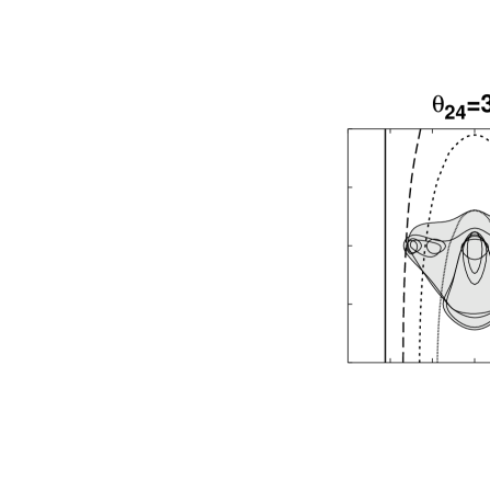
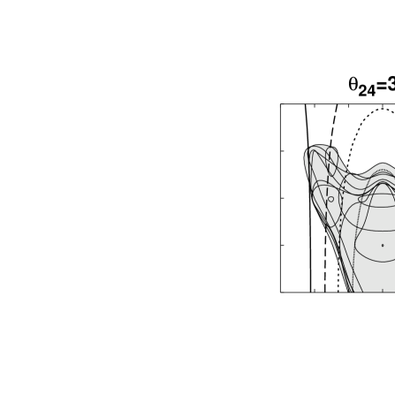
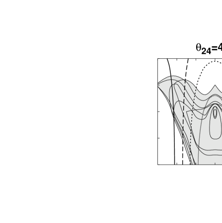
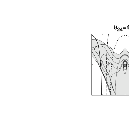
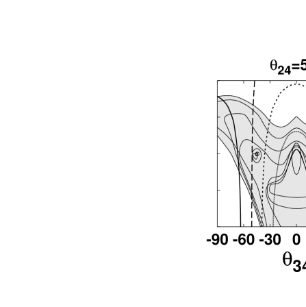
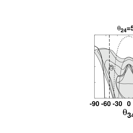
                                                                                       The shadowed area is the allowed region projected on the $(\theta_{34},~{}\theta_{23})$ plane for various values of $\Delta m_{43}^{2}$ ($10^{-3.5}$eV${}^{2}\leq\Delta m_{43}^{2}\leq 10^{-2}$eV²) for each value of $\theta_{24}=30^{\circ},\cdots,55^{\circ}$, respectively, and the thin solid lines are boundary of the allowed region for various values of $\Delta m_{43}^{2}$. The solid, dashed, coarse dotted and fine dotted lines stand for the contours of $c_{s}\equiv|U_{s1}|^{2}+|U_{s2}|^{2}$ =$|c_{23}c_{34}+s_{23}s_{24}s_{34}e^{i\delta_{1}}|^{2}=0.2,0.4,0.6,0.8$, respectively. Solutions with $c_{s}\raisebox{0.85358pt}{\em$\,<$}\raisebox{-5.12149pt}{\em$\sim\,$}0.2$ exist for $40^{\circ}\raisebox{0.85358pt}{\em$\,<$}\raisebox{-5.12149pt}{\em$\sim\,$}\theta_{24}\raisebox{0.85358pt}{\em$\,<$}\raisebox{-5.12149pt}{\em$\sim\,$}55^{\circ}$ and they can have Large Mixing Angle solutions of the solar neutrino problem.

Figure 2: Allowed region at 90%CL for $\delta_{1}=\pi/2$.

3 Analysis of the atmospheric neutrino data

I calculate the disappearance probability $P(\nu_{\mu}\rightarrow\nu_{\mu})$ by solving (23) numerically, and evaluate the number of events. Then I define $\chi^{2}$ as

$$\chi^{2}=\chi_{\rm sub-GeV}^{2}+\chi_{\rm multi-GeV}^{2}+\chi_{\rm through}^{2}$$ (31)

where $\chi_{\rm sub-GeV}^{2}$, $\chi_{\rm multi-GeV}^{2}$ and $\chi_{\rm through}^{2}$ are $\chi^{2}$ for sub-GeV, multi-GeV, and upward going through $\mu$ events, respectively. I have evaluated $\chi^{2}$ for $\theta_{24}=(25+5j)^{\circ}$ ($j=0,\cdots,7$), $\theta_{34}=15j^{\circ}$ ($j=-6,\cdots,6$), $\theta_{23}=10j^{\circ}$ ($j=0,\cdots,4$), $\delta_{1}=0^{\circ},45^{\circ},90^{\circ}$, $\Delta m^{2}_{43}=10^{-4+j/10}$eV² ($j=5,\cdots,20$) and it is found that $\chi^{2}$ has the minimum value $\chi^{2}_{\rm min}=43.1$ $(\chi_{\rm sub-GeV}^{2}=19.0$, $\chi_{\rm multi-GeV}^{2}=13.2$, $\chi_{\rm through}^{2}=11.6$) for $\Delta m_{43}^{2}=10^{-2.9}{\rm eV}^{2}=1.3\times 10^{-3}{\rm eV}^{2}$, $(\theta_{24},\theta_{34},\theta_{23})=(35^{\circ},15^{\circ},20^{\circ})$, $\delta_{1}=0$ with 45 degrees of freedom. For pure $\nu_{\mu}\leftrightarrow\nu_{\tau}$ ($\theta_{34}=\theta_{23}=0$), the best fit is obtained $\chi^{2}_{\rm min}(\nu_{\mu}\leftrightarrow\nu_{\tau})=48.3$, $(\chi_{\rm sub-GeV}^{2}=19.8,\chi_{\rm multi-GeV}^{2}=17.0,\chi_{\rm through}^{2}=10.6)$ for $\Delta m_{43}^{2}=2.0\times 10^{-3}{\rm eV}^{2}$, $(\theta_{24},\theta_{34},\theta_{23})=(40^{\circ},0^{\circ},0^{\circ})$. The allowed regions at 90%CL are obtained by $\chi^{2}\leq\chi^{2}_{\rm min}+\Delta\chi^{2}$, where $\Delta\chi^{2}$=9.2 for five degrees of freedom. In Fig.2 the allowed region at 90% confidence level is depicted as a shadowed area in the $(\theta_{34},~{}\theta_{23})$ plane for various values of $\Delta m_{43}^{2}$ ($10^{-3.5}$eV${}^{2}\leq\Delta m_{43}^{2}\leq 10^{-2}$eV²) for each value of $\theta_{24}=30^{\circ},\cdots,55^{\circ}$ and for $\delta_{1}=\pi/2$, together with lines $c_{s}$=constant. A few remarks are in order. (1) Pure $\nu_{\mu}\leftrightarrow\nu_{s}$ oscillation, which is given by $\theta_{34}=\pm 90^{\circ}$,  $\theta_{23}=0$, is excluded at 99.7%CL for any value of $\Delta m_{43}^{2}$, $\theta_{24}$, $\delta_{1}$ and this is consistent with the claim [3] by the Superkamiokande group. (2) For generic value of $(\theta_{34},~{}\theta_{23})$, the oscillation is hybrid not only with $\nu_{\mu}\leftrightarrow\nu_{\tau}$ and $\nu_{\mu}\leftrightarrow\nu_{s}$ but also with $\Delta m_{43}^{2}$ and $\Delta m_{32}^{2}$. To illustrate this, let me give the expressions of oscillation probability in vacuum in the case of $\delta_{1}=\pi/2$:

$$P(\nu_{\mu}\rightarrow\nu_{\tau}) = 2c_{24}^{2}s_{23}^{2}(c_{23}^{2}s_{34}^{2}+s_{23}^{2}s_{24}^{2}c_{34}^{2})$$

$$+ c_{23}^{2}c_{34}^{2}\sin^{2}2\theta_{24}\sin^{2}\left({\Delta m_{43}^{2}L\over 4E}\right)$$

$$P(\nu_{\mu}\rightarrow\nu_{s}) = 2c_{24}^{2}s_{23}^{2}(c_{23}^{2}c_{34}^{2}+s_{23}^{2}s_{24}^{2}s_{34}^{2})$$

$$+ c_{23}^{2}s_{34}^{2}\sin^{2}2\theta_{24}\sin^{2}\left({\Delta m_{43}^{2}L\over 4E}\right)$$

$$P(\nu_{\mu}\rightarrow\nu_{\mu}) = 1-2c_{24}^{2}s_{23}^{2}\left(1-c_{24}^{2}s_{23}^{2}\right)-c_{23}^{2}$$ (32)

$$\times \sin^{2}2\theta_{24}\sin^{2}\left({\Delta m_{43}^{2}L\over 4E}\right),$$

where I have averaged over rapid oscillations due to $\Delta m_{32}^{2}$. As is seen in (32), roughly speaking, $\theta_{34}$ represents the ratio of $\nu_{\mu}\leftrightarrow\nu_{\tau}$ and $\nu_{\mu}\leftrightarrow\nu_{s}$, whereas $\theta_{23}$ indicates the contribution of $\sin^{2}(\Delta m_{32}^{2}L/4E)$ in oscillations. Zenith angle dependence of the $\mu$-like multi-GeV events and the upward going through $\mu$ events are shown in Fig.3 for a few sets of the oscillation parameters. The disappearance probability behaves like $1-P(\nu_{\mu}\rightarrow\nu_{\mu})=\alpha+\beta\sin^{2}(\Delta m_{43}^{2}L/4E)$ ($\alpha$, $\beta$ are constant) and $\alpha>0$ is satisfied whenever $\theta_{23}\neq 0$. Because of this constant $\alpha$, which never appears in the analysis of the two flavor framework, the fit for $\theta_{23}\neq 0$ tends to be better than in the case of $\theta_{23}=0$. The reason why the best fit point is slightly away from pure $\nu_{\mu}\leftrightarrow\nu_{\tau}$ case and the reason why an exotic solution like ($\theta_{24}$, $\theta_{23}$, $\theta_{34}$) =($45^{\circ}$, $30^{\circ}$, $90^{\circ}$), $\delta_{1}=90^{\circ}$, $\Delta m_{43}^{2}$=1.3$\times 10^{-3}$eV² is allowed is because a better fit to the multi-GeV contained events compensates a worse fit to the upward going through $\mu$ events, and in total the case of hybrid oscillations fits better to the data (Notice that the fit of $\nu_{\mu}\leftrightarrow\nu_{s}$ scenario to the contained events is known to be good [16, 17] and in the present case the fit becomes even better due to the presence of $\alpha$).

Figure 3: Zenith angle dependence

4 Conclusions

I have shown in the framework of four neutrino oscillations without assuming the BBN constraints that the Superkamiokande atmospheric neutrino data are explained by wide range of the oscillation parameters which implies hybrid oscillations with $\nu_{\mu}\leftrightarrow\nu_{\tau}$ and $\nu_{\mu}\leftrightarrow\nu_{s}$ as well as with $\Delta m_{\mbox{\rm\scriptsize atm}}^{2}$ and $\Delta m_{\mbox{\rm\scriptsize LSND}}^{2}$. The case of pure $\nu_{\mu}\leftrightarrow\nu_{s}$ is excluded at 3.0$\sigma$CL in good agreement with the Superkamiokande analysis. It is found by combining the analysis on the solar neutrino data by Giunti, Gonzalez-Garcia and Peña-Garay that the LMA and VO solutions as well as SMA solution of the solar neutrino problem are allowed.

References

• [1] B.T. Cleveland et al., Nucl. Phys. B (Proc. Suppl.) 38, 47 (1995); Y. Fukuda et al., Phys. Rev. Lett. 77, 1683 (1996) and references therein; Y. Suzuki, Nucl. Phys. B (Proc. Suppl.) 77, 35 (1999) and references therein; V.N. Gavrin, Nucl. Phys. B (Proc. Suppl.) 77, 20 (1999) and references therein; T.A. Kirsten, Nucl. Phys. B (Proc. Suppl.) 77, 26 (1999) and references therein.
• [2] K.S. Hirata et al., Phys. Lett. B280, 146 (1992); Y. Fukuda et al., Phys. Lett. B335, 237 (1994); S. Hatakeyama et al., Phys. Rev. Lett. 81, 2016 (1998); R. Becker-Szendy et al., Phys. Rev. D46, 3720 (1992) and references therein; T. Kajita, Nucl. Phys. (Proc. Suppl.) 77, 123 (1999) and references therein; Y. Fukuda et al., Phys. Rev. Lett. 82, 2644 (1999); W.W.M. Allison et al., Phys. Lett. B449, 137 (1999); T. Kafka, hep-ex/9912060; M. Spurio, Nucl. Phys. (Proc. Suppl.) 85 37 (2000).
• [3] T. Toshito, talk given at YITP Workshop on Theoretical Problems related to Neutrino Oscillations, 28 February – 1 March, 2000, Kyoto, Japan.
• [4] D.H. White, Nucl. Phys. (Proc. Suppl.) 77 207 (1999) and references therein.
• [5] N. Okada and O. Yasuda, Int. J. Mod. Phys. A 12, 3669 (1997).
• [6] S.M. Bilenky, C. Giunti, W. Grimus and T. Schwetz, Astropart. Phys. 11, 413 (1999).
• [7] S. Goswami, Phys. Rev. D 55, 2931 (1997).
• [8] B. Ackar et al., Nucl. Phys. B434, 503 (1995).
• [9] C.J. Copi, D.N. Schramm and M. S. Turner, Phys. Rev. Lett. 75, 3981 (1995); K.A. Olive and G. Steigman, Phys. Lett. B354, 357 (1995); P.J. Kernan and S. Sarkar, Phys. Rev. D 54, R3681 (1996); S. Sarkar, Rep. on Prog. in Phys. 59, 1 (1996).
• [10] C. Giunti, M. C. Gonzalez-Garcia and C. Peña-Garay, hep-ph/0001101.
• [11] O. Yasuda, hep-ph/0006319.
• [12] S.M. Bilenky, C. Giunti and W. Grimus, hep-ph/9609343; Eur. Phys. J. C1, 247 (1998).
• [13] L. Borodovsky et al., Phys. Rev. Lett. 68, 274 (1992).
• [14] Review of Particle Physics, Particle Data Group, Eur. Phys. J. C3, 1 (1998).
• [15] F. Dydak et al., Phys. Lett. B 134, 281 (1984).
• [16] R. Foot, R.R. Volkas and O. Yasuda, Phys. Rev. D58, 13006 (1998); O. Yasuda, Nucl. Phys. B (Proc. Suppl.) 77, 146 (1999).
• [17] M.C. Gonzalez-Garcia, H. Nunokawa, O.L.G. Peres and J.W.F. Valle, Nucl. Phys. B543, 3 (1999).