Complete one-loop corrections to $e^{+}e^{-}\to W^{+}W^{-}$ in the MSSM

Abstract

The complete $\mathcal{O}(\alpha)$ corrections including soft-photon bremsstrahlung to the process $e^{+}e^{-}\to W^{+}W^{-}$ in the MSSM are calculated for on-shell W bosons. The relative difference between the MSSM and Standard Model corrections is generally quite small. The maximum deviation from the Standard Model within the scanned region of parameter space is $\lesssim 1.5\%$ for unpolarized and transversally polarized W bosons, and $\lesssim 2.7\%$ for longitudinal W bosons.
PACS numbers: 12.60.Jv, 13.10.+q, 12.15.Lk.

1 Introduction

The process $e^{+}e^{-}\to W^{+}W^{-}$ is already one of the key processes at LEP2, and will be of similar importance at future linear $e^{+}e^{-}$ colliders. Hence it is not surprising that considerable theoretical effort has gone into the precise prediction of the cross-section in the Standard Model (SM), both for on- and off-shell W bosons ([3], see [4] for a review).

For a process well accessible both experimentally and theoretically in the SM, one of the obvious questions to ask is whether it can tell us anything about physics beyond the SM. Supersymmetric extensions play a special role because they, like the SM, allow to make precise predictions in terms of a set of input parameters. Previous calculations in supersymmetric theories include the complete one-loop corrections in spontaneously broken supersymmetry [5], sfermion-loop effects in the MSSM [6, 7], and also the complete MSSM corrections to the closely related triple-gauge-boson vertex [8].

In this paper the complete one-loop corrections for $e^{+}e^{-}\to W^{+}W^{-}$ in the MSSM including real bremsstrahlung in the soft-photon approximation are presented. The results are rather small: the maximum deviation from the Standard Model within the scanned region of parameter space is $\lesssim 1.5\%$ for unpolarized and transversally polarized W bosons, and $\lesssim 2.7\%$ for longitudinal W bosons.

The outline of this paper is as follows. In Sect. 2 the kinematics and notation are fixed. Sect. 3 describes the details of the one-loop calculation. The results of the calculation and the scan over the MSSM parameter space are presented in Sect. 4. Sect. 5 finally gives the conclusions.

2 Kinematics and notation

The reaction studied here is

$$e^{+}(k_{1},\lambda_{1})+e^{-}(k_{2},\lambda_{2})\to W^{+}(k_{3},\lambda_{3})+W^{-}(k_{4},\lambda_{4})\,,$$ (1)

where $k_{i}$ and $\lambda_{i}$ represent the momenta and helicities of the external particles, respectively.

The incoming particles travel along the $z$ axis and are scattered into the $x$–$z$ plane. Neglecting the electron mass, the explicit representations of the momenta and the polarization vectors in the centre-of-mass system are

$$k_{1}^{\mu} =E\left(1,\,0,\,0,\,-\beta\right), \varepsilon_{3}^{\mu}(0) =\left(-p,\,E\sin\theta,\,0,\,E\cos\theta\right)/M_{W}\,,$$ (2)

$$k_{2}^{\mu} =E\left(1,\,0,\,0,\,\beta\right), \varepsilon_{3}^{\mu}(\pm) =\left(0,\,-\cos\theta,\,\pm\mathrm{i},\,\sin\theta\right)/\sqrt{2}\,,$$

$$k_{3}^{\mu} =\left(E,\,-p\sin\theta,\,0,\,-p\cos\theta\right),\qquad \varepsilon_{4}^{\mu}(0) =\left(-p,\,-E\sin\theta,\,0,\,-E\cos\theta\right)/M_{W}\,,$$

$$k_{4}^{\mu} =\left(E,\,p\sin\theta,\,0,\,p\cos\theta\right), \varepsilon_{4}^{\mu}(\pm) =\left(0,\,\cos\theta,\,\pm\mathrm{i},\,-\sin\theta\right)/\sqrt{2}\,,$$

where $\beta$ is the velocity of the electrons, $p=\sqrt{E^{2}-M_{W}^{2}}$ is the momentum of the W bosons, $E=\sqrt{s}/2$ is the beam energy, and $\theta$ is the scattering angle.

The polarized differential cross-section is obtained from the helicity amplitudes $\mathcal{M}$ as

$$\left(\frac{\mathrm{d}\sigma}{\mathrm{d}\Omega}\right)_{\lambda_{1}\lambda_{2}\lambda_{3}\lambda_{4}}=\frac{1}{64\pi^{2}s}\left|\mathcal{M}_{\lambda_{1}\lambda_{2}\lambda_{3}\lambda_{4}}\right|^{2}.$$ (3)

In the following, only unpolarized electrons are considered, since that is the situation at LEP2. In this case the cross-section has to be averaged over the initial helicities according to

$$\left(\frac{\mathrm{d}\sigma}{\mathrm{d}\Omega}\right)_{\text{UU}\lambda_{3}\lambda_{4}}=\frac{1}{4}\sum_{\lambda_{1},\lambda_{2}=\pm 1}\left(\frac{\mathrm{d}\sigma}{\mathrm{d}\Omega}\right)_{\lambda_{1}\lambda_{2}\lambda_{3}\lambda_{4}}.$$ (4)

Polarization combinations are given by a sequence of four letters, e.g. UULT, where L, T, and U denote longitudinal ($\lambda=0$), transverse ($\lambda=\pm$), and unpolarized particles.

3 One-loop corrections

Since the coupling of the electron to any of the Higgs particles in the SM or the MSSM is suppressed by a factor $m_{e}/M_{W}$, the Higgs-exchange diagrams can safely be neglected. The tree-level diagrams are then the same for the SM and the MSSM, i.e. $\gamma$ and $Z$ exchange in the $s$-channel and neutrino exchange in the $t$-channel (see Fig. 1). The tree-level results shall not be discussed here as this has been done in detail elsewhere (explicit formulas can be found e.g. in [4]).

Figure 1: The tree-level diagrams.

3.1 Calculational framework

The calculation of the $\mathcal{O}(\alpha)$ radiative corrections has been performed in ’t Hooft–Feynman gauge. Ultraviolet (UV) divergences were treated within dimensional regularization. For the renormalization the on-shell scheme [9] was used, following the formulation worked out in [10]. In the absence of SUSY particles at tree level, only those counter-terms appear that are already present in the SM. The only change is that now the self-energies from which the renormalization constants are derived have to be calculated in the MSSM.

To $\mathcal{O}(\alpha)$, the squared matrix element is given by

$$|\mathcal{M}|^{2}=|\mathcal{M}_{\text{Born}}|^{2}(1+\delta_{\text{soft}})+2\mathop{\rm Re}\left(\mathcal{M}_{\text{Born}}^{*}\mathcal{M}_{\text{1-loop}}\right)\,,$$ (5)

where $\mathcal{M}_{\text{Born}}$ and $\mathcal{M}_{\text{1-loop}}$ denote the sum of the contributing tree-level and one-loop Feynman diagrams, respectively, and $\delta_{\text{soft}}$ is the QED correction factor from real bremsstrahlung in the soft-photon approximation.

The Feynman diagrams were generated with FeynArts [11] which in its current version uses algorithms that can deal with supersymmetric theories [12]. The resulting amplitudes were algebraically simplified using FormCalc [13] and then converted to a Fortran program. The LoopTools package [13, 14] was used to evaluate the one-loop scalar and tensor integrals. For a single point in phase and parameter space the Fortran program runs about 3.6 ms in the SM and 102 ms in the MSSM. Scans over parameter space in the MSSM typically take several hours.

Apart from obvious checks such as UV- and IR-finiteness, the SM results of [4] were fully confirmed and the effects of sfermion-loops in [6] could be reproduced for various scenarios of sfermion masses to within a very small constant shift ($\sim.5\%$) which is an effect of the different renormalization schemes used and hence of higher order.

With the presence of external gauge bosons one might expect sizable gauge cancellations and hence instabilities in the numerical code. To safeguard against such problems, the SM values were computed once in the conventional way and once in the background-field method [15], where gauge cancellations should be greatly reduced, and an agreement to 9 digits was found. Even though the same comparison cannot easily be done for the MSSM (a corresponding model file is currently not available), a similar stability is expected since the gauge structure of the MSSM is essentially the same as in the SM. As an alternative measure of stability, one can compare the individual contributions from self-energies, vertices, and boxes with their sum. To show that the cancellations are harmless numerically, the following table lists the individual contributions (each of them renormalized) that make up the amplitude at a particular point in parameter space for longitudinal W bosons, for which the largest cancellations can be expected.

$$\left.\frac{1}{64\pi^{2}s}2\mathop{\rm Re}\mathcal{M}_{\text{Born}}^{*}\mathcal{M}_{X}\right|_{\begin{subarray}{l}\sqrt{s}=500\,\text{GeV}\\ \theta=90^{\circ}\end{subarray}}=\left\{\begin{array}[]{lr}X=\text{self-energies:}&-.02535074~{}\text{pb}\\ X=\text{vertices:}&-.03675248~{}\text{pb}\\ X=\text{boxes:}&.06422023~{}\text{pb}\\ \hline\cr X=\text{sum:}&.00211700~{}\text{pb}\end{array}\right.$$ (6)

3.2 QED corrections

In addition to the virtual diagrams, real photon emission from the external legs has to be taken into account to cancel the infrared (IR) divergences which arise from the exchange of massless photons. The IR divergences are regularized by an infinitesimal photon mass $\lambda$. In the soft-photon limit the cross-section for real photon emission is proportional to the Born cross-section,

$$\left(\frac{\mathrm{d}\sigma}{\mathrm{d}\Omega}\right)_{\text{soft}}=\left(\frac{\mathrm{d}\sigma}{\mathrm{d}\Omega}\right)_{\text{Born}}\delta_{\text{soft}}\,,$$ (7)

with the soft-photon factor $\delta_{\text{soft}}$ given by

$$\delta_{\text{soft}}=-\frac{e^{2}}{(2\pi)^{3}}\int\limits_{k_{0}\leqslant\Delta E}\frac{\mathrm{d}^{3}k}{2k_{0}}\left.\sum_{i,j=1}^{4}\frac{\pm Q_{i}Q_{j}(k_{i}k_{j})}{(k_{i}k)(k_{j}k)}\right|_{k_{0}=\sqrt{k^{2}+\lambda^{2}}}\,.$$ (8)

Here $\Delta E$ is the maximum energy of the emitted photons, $Q_{i}$ is the charge of the $i$th external particle, and the sign in front of the product $Q_{i}Q_{j}$ is $+$ if particles $i$ and $j$ are both either incoming or outgoing, and $-$ otherwise. The basic integrals needed for the evaluation of (8) have been worked out e.g. in [16].

The absolute magnitude of the $\mathcal{O}(\alpha)$ corrections is largely determined by the QED contributions and depends strongly on the photon-energy cutoff $\Delta E$ through logarithms of the form $\log\Delta E/E$. Without an experimentally motivated choice of $\Delta E$, the overall size of the one-loop corrections can be shifted more or less at will using different values of $\Delta E$. Since the intention here is only to show the differences between the SM and the MSSM calculations, the concrete value of $\Delta E$ is rather unimportant. In this calculation a soft-photon cutoff energy of $\Delta E=0.05\sqrt{s}$ has been used as in [4].

The cancellation of the IR divergences has been checked numerically by varying the photon-mass $\lambda$ on which the result must not depend. A variation of $\lambda$ from 1 to $10^{10}$ GeV leaves the first 10 digits of the cross-section invariant.

While soft-photon radiation is sufficient to cancel IR divergences, it is an approximation, valid only if $\Delta E$ is small compared to all relevant energy scales. If this is not the case, hard-photon radiation must be taken into account, too. However, the hard-photon corrections at $\mathcal{O}(\alpha)$ are exactly the same as in the SM, therefore they have been omitted in the present calculation.

3.3 Inventory of one-loop diagrams

This section lists the contributing one-loop diagrams. The diagrams can be separated into self-energy contributions, vertex corrections, and box corrections. Note that diagrams which are already present in the SM are omitted in the figures.

The self-energy contributions fall into two categories, corrections to the $\gamma$ and $Z$ propagator in the $s$-channel, and corrections to the $\nu$ propagator in the $t$-channel. These diagrams are shown in Fig. 2.

Figure 2: The MSSM self-energy corrections. Braces indicate that there is one diagram for the first members of all braced lists, one for the second members, etc. A sfermion with index $i$ accounts for six particles, e.g. $\tilde{e}_{i}=\{\tilde{e}^{1},\tilde{e}^{2},\tilde{\mu}^{1},\tilde{\mu}^{2},\tilde{\tau}^{1},\tilde{\tau}^{2}\}$.

The vertex diagrams can be grouped into corrections to the initial- and final-state vertex in the $s$-channel (Figs. 3 and 4), and corrections to the $t$-channel vertices (Fig. 5).

Figure 3: The MSSM contributions to the initial-state vertex in the $s$-channel.

Figure 4: The MSSM contributions to the $s$-channel final-state vertex. Braces indicate that there is one diagram for the first members of all braced lists, one for the second members, etc. A sfermion with index $i$ accounts for six particles, e.g. $\tilde{e}_{i}=\{\tilde{e}^{1},\tilde{e}^{2},\tilde{\mu}^{1},\tilde{\mu}^{2},\tilde{\tau}^{1},\tilde{\tau}^{2}\}$.

Finally, the box diagrams are displayed in Fig. 6.

Figure 5: The MSSM contributions to the $t$-channel vertices.

Figure 6: The MSSM box diagrams.

4 Numerical results

4.1 Input parameters

4.1.1 Standard Model parameters

For the SM parameters the following numerical values are used:

$$\alpha^{-1} =137.0359895,\quad M_{Z} =91.1867\text{ GeV},\quad M_{W} =80.39\text{ GeV},$$ (9)

$$m_{e} =0.51099907\text{ MeV},\quad m_{u} =53.8\text{ MeV},\quad m_{d} =53.8\text{ MeV},\quad$$

$$m_{\mu} =105.658389\text{ MeV}, m_{c} =1.50\text{ GeV}, m_{s} =150\text{ MeV},$$

$$m_{\tau} =1777\text{ MeV}, m_{t} =174\text{ GeV}, m_{b} =4.7\text{ GeV}.$$

The masses of the up and down quarks are effective parameters which are adjusted such that the five-flavour hadronic contribution to $\Delta\alpha$ is 0.02778 [17], i.e.

$$\Delta\alpha_{\text{had}}^{(5)}(s=M_{Z}^{2})=\frac{\alpha}{\pi}\sum_{f=u,c,d,s,b}q_{f}^{2}\Bigl{(}\log\frac{M_{Z}^{2}}{m_{f}^{2}}-\frac{5}{3}\Bigr{)}\overset{!}{=}0.02778\,.$$

4.1.2 MSSM parameters

Higgs sector

The neutral Higgs sector is fixed by choosing a value for $\tan\beta$ and for the mass $M_{A^{0}}$ of the CP-odd neutral Higgs boson $A^{0}$. For the other neutral-Higgs masses, which receive significant radiative corrections [18], the two-loop approximation formula of [19] is used.

There are only small radiative corrections for the charged Higgs masses and the following equation holds for $M_{A^{0}}\sim\mathcal{O}(M_{W})$ [20].

$$M_{H^{\pm}}^{2}=M_{A^{0}}^{2}+M_{W}^{2}+\frac{5\alpha M_{W}^{2}}{2\pi c_{W}^{2}}\ln\frac{M_{\text{SUSY}}}{M_{W}}\\ +\frac{3\alpha}{4\pi s_{W}^{2}M_{W}^{2}}\left[\frac{2m_{t,r}^{2}m_{b}^{2}}{\sin^{2}\!\beta\cos^{2}\!\beta}-M_{W}^{2}\left(\frac{m_{t,r}^{2}}{\sin^{2}\!\beta}+\frac{m_{b}^{2}}{\cos^{2}\!\beta}\right)+\frac{2}{3}M_{W}^{4}\right]\ln\frac{M_{\text{SUSY}}}{m_{t,r}}\,,$$ (10)

where $M_{\text{SUSY}}$ is a universal soft-SUSY-breaking mass introduced in the next paragraph and $m_{t,r}=m_{t}(1+4\alpha_{s}(m_{t})/3\pi)^{-1}$ is the running top mass.

Sfermions

For simplicity, all soft-SUSY-breaking parameters are assumed equal and mixing between sfermion generations is neglected, so that

$$\begin{gathered}M_{\tilde{Q}}^{2}=M_{\tilde{U}}^{2}=M_{\tilde{D}}^{2}=M_{\tilde{L}}^{2}=M_{\tilde{E}}^{2}=M_{\text{SUSY}}^{2}{\rm 1\mskip-4.25mul}\,,\\ A_{U}=A_{u}{\rm 1\mskip-4.25mul}\,,\qquad A_{L}=A_{D}=A_{d}{\rm 1\mskip-4.25mul}\,.\end{gathered}$$ (11)

Then, the sfermion mass matrix is given by [21, 22]

$$\begin{pmatrix}M_{\text{SUSY}}^{2}+M_{Z}^{2}\cos(2\beta)(I_{3}^{f}-Q_{f}s_{W}^{2})+m_{f}^{2}&m_{f}(A_{\{u,d\}}-\mu\{\cot\beta,\tan\beta\})\\ m_{f}(A_{\{u,d\}}-\mu\{\cot\beta,\tan\beta\})&M_{\text{SUSY}}^{2}+M_{Z}^{2}\cos(2\beta)Q_{f}s_{W}^{2}+m_{f}^{2}\end{pmatrix}$$ (12)

where the elements in braces apply to $I_{3}^{f}=+\frac{1}{2}$ and $-\frac{1}{2}$, respectively.

Charginos and Neutralinos

The chargino mass matrix [21, 22]

$$X=\begin{pmatrix}M_{2}&\sqrt{2}M_{W}\sin\beta\\ \sqrt{2}M_{W}\cos\beta&\mu\end{pmatrix}$$ (13)

and the neutralino mass matrix [21, 22]

$$Y=\begin{pmatrix}M_{1}&0&-M_{Z}s_{W}\cos\beta&M_{Z}s_{W}\sin\beta\\ 0&M_{2}&M_{Z}c_{W}\cos\beta&-M_{Z}c_{W}\sin\beta\\ -M_{Z}s_{W}\cos\beta&M_{Z}c_{W}\cos\beta&0&-\mu\\ M_{Z}s_{W}\sin\beta&-M_{Z}c_{W}\sin\beta&-\mu&0\end{pmatrix}$$ (14)

are diagonalized with unitary matrices $U$, $V$, and $N$ such that

$$\begin{gathered}U^{*}XV^{-1}=\mathop{\rm diag}(m_{\tilde{\chi}_{1}},m_{\tilde{\chi}_{2}})\,,\\ N^{*}YN^{-1}=\mathop{\rm diag}(m_{\tilde{\chi}^{0}_{1}},\ldots,m_{\tilde{\chi}^{0}_{4}})\,.\end{gathered}$$ (15)

This diagonalization is done numerically using the subroutines of the LAPACK library [23]. The $U(1)$ gaugino-mass parameter $M_{1}$ which appears as a further input parameter in $Y$ is fixed, as usual, by the SUSY-GUT relation

$$M_{1}=\frac{5}{3}\frac{s_{W}^{2}}{c_{W}^{2}}M_{2}\,.$$ (16)

4.1.3 Parameter scan

The remaining input parameters are then scanned over the following regions:

$$\begin{array}[]{c|c}\text{SM}&\text{MSSM}\\ \hline\cr M_{H}=100\dots 300\text{ GeV}&\begin{aligned} \tan\beta&=1.5,5,50\\ M_{A^{0}}&=100\dots 1000\text{ GeV}\\ \mu&=-1000\dots 1000\text{ GeV}\\ M_{2}&=100\dots 1000\text{ GeV}\\ M_{\text{SUSY}}&=100\dots 1000\text{ GeV}\\ A_{u}=A_{d}&=M_{\text{SUSY}},2M_{\text{SUSY}}\end{aligned}\end{array}$$ (17)

When the particle masses are calculated from these input parameters, the Fortran program checks whether they are consistent with the current exclusion limits and automatically omits already-excluded points in parameter space from the scan. The following bounds are used:

$$M_{\tilde{t}} \geqslant 80\text{ GeV}~{}\cite[cite]{[\@@bibref{}{squarkbounds}{}{}]}\,,\qquad M_{h^{0}} \geqslant 85\text{ GeV}~{}\cite[cite]{[\@@bibref{}{h0bounds}{}{}]}\,,$$ (18)

$$M_{\tilde{b}} \geqslant 70\text{ GeV}~{}\cite[cite]{[\@@bibref{}{squarkbounds}{}{}]}\,, m_{\tilde{\chi}^{0}} \geqslant 30\text{ GeV}~{}\cite[cite]{[\@@bibref{}{chibounds}{}{}]}\,,$$

$$M_{\tilde{q}\neq\tilde{b},\tilde{t}} \geqslant 150\text{ GeV}~{}\cite[cite]{[\@@bibref{}{squarkbounds}{}{}]}\,, m_{\tilde{\chi}} \geqslant 90\text{ GeV}~{}\cite[cite]{[\@@bibref{}{chibounds}{}{}]}\,.$$

$$M_{\tilde{\ell}} \geqslant 70\text{ GeV}~{}\cite[cite]{[\@@bibref{}{sleptonbounds}{}{}]}\,,$$

4.2 Results

In Fig. 7 the absolute values of the total and differential cross-section in the SM and MSSM is shown for three different polarizations: UUUU (all particles unpolarized), UUTT (transverse W bosons), and UULL (longitudinal W bosons). The thickness of the curves reflects the range of the allowed values within the parameter scan (17).

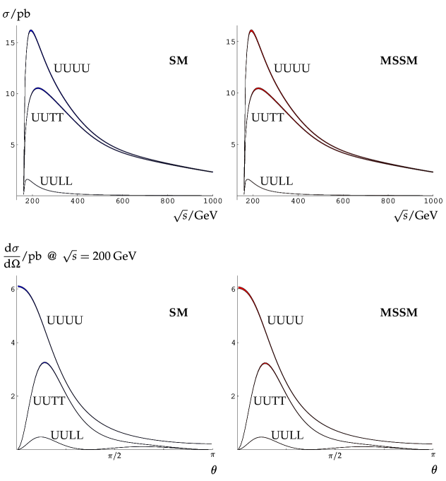
Figure 7: The total cross-section and the differential cross-section at $\sqrt{s}=200$ GeV for the SM and the MSSM. The thickness of the curves give the range of allowed values within the parameter scan (17). The polarizations are denoted by: UUUU (all particles unpolarized), UUTT (transverse W bosons), and UULL (longitudinal W bosons).

Fig. 8 shows the relative corrections in the SM and MSSM with respect to the Born cross-section. The overall magnitude of the corrections is largely determined by the well-understood QED logarithms, as discussed in Sect. 3.2. The bands show the variation of the cross-section within the parameter scan (17). The bands for the SM and MSSM overlap slightly, the MSSM band being the lower one. The two bands are of comparable width of the order of a few percent for all polarizations. The dominating polarizations over the entire energy range are UU$\pm$$\mp$, and this explains why the plots for the UUUU and UUTT polarizations in Fig. 8 are quite similar. On the other hand it is not possible to trace the origins of the radiative corrections by disentangling the self-energy, vertex, and box contributions since in the presence of external gauge bosons there are delicate gauge cancellations.

Figure 8: The relative difference between the one-loop corrected and the Born cross-section. The cross-hatched bands indicate the minimum and maximum reached within the scan over the parameter space (17). The polarizations are denoted by: UUUU (all particles unpolarized), UUTT (transverse W bosons), and UULL (longitudinal W bosons).

The relative deviation between the SM central value and the MSSM band is plotted in Fig. 9. While the largest corrections ($\sim-2.7\%$ at 1 TeV) are seen for purely longitudinal W bosons, one has to keep in mind that the cross-section for longitudinally polarized W bosons is much smaller than for the transverse polarizations. In the transverse polarizations and in the unpolarized case the maximum deviation between the SM and the MSSM is roughly 1.5%. The maximum deviation is reached in all polarizations for light SUSY particles, for example in the unpolarized case (UUUU) the lightest higgs, stop, chargino, and neutralino masses at the point of maximum deviation are $M_{h^{0}}=91\text{ GeV}$, $M_{\tilde{t}}=165\text{ GeV}$, $m_{\tilde{\chi}}=117\text{ GeV}$, and $m_{\tilde{\chi}^{0}}=52\text{ GeV}$, respectively.

Figure 9: The relative difference between the SM central value $\bar{\sigma}_{\text{1-loop}}^{\text{SM}}$ and the MSSM bands of Fig. 8. The polarizations are denoted by: UUUU (all particles unpolarized), UUTT (transverse W bosons), and UULL (longitudinal W bosons).

The variation of the cross-section with the scanned MSSM parameters is shown in Fig. 10. The largest variation is connected with the soft-SUSY-breaking mass $M_{\text{SUSY}}$ and confirms the idea of the previous calculations [6, 7] that important contributions come from the sfermion sector. Nevertheless, the contributions from the other sectors are similar in size and cannot be neglected.

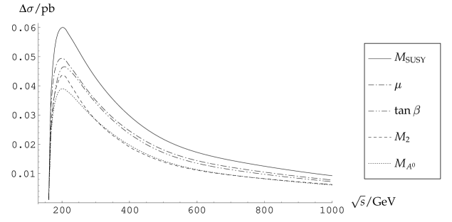
Figure 10: The variation of the MSSM cross-section for unpolarized particles with the scanned MSSM parameters. The variation of a parameter $X$ is computed as the difference between maximum and minimum of the cross-section for fixed $X$, averaged over all values of $X$.

The calculation was checked for a possible scheme dependence by repeating it using the input values $\{\alpha,G_{F},M_{Z}\}$ instead of $\{\alpha,M_{W},M_{Z}\}$. This is not entirely straightforward since $M_{W}$ enters not only in loop corrections, but more directly in the kinematics of the process. For instance, the threshold of $2M_{W}$ is different in the SM and MSSM so that it is not admissible to plot the ratio as in Fig. 9. To compute $M_{W}(\alpha,G_{F},M_{Z})$, the fit formula of [28], approximating the two-loop result, together with the MSSM contributions to $\Delta\rho$ [29] have been used. The results are shown for longitudinal W bosons, for which the MSSM corrections are largest, in Fig. 11 and differ only slightly from the former result.

Figure 11: The same as the lower diagram in Fig. 8 (i.e. the relative one-loop corrections for longitudinal W bosons), but calculated from the input parameter set $\{\alpha,G_{F},M_{Z}\}$ instead of $\{\alpha,M_{W},M_{Z}\}$. The cross-hatched bands indicate the minimum and maximum reached within the scan over the parameter space (17).

5 Conclusions

The MSSM corrections to $e^{+}e^{-}\to W^{+}W^{-}$ are probably too small to be detected at LEP2, taking into account that the convolution with decay amplitudes in the final and photon radiation in the initial state tends to smear the corrections.

With the projected accuracy of a linear collider, however, corrections of this magnitude will play a role. Yet even a linear collider may have a hard time disentangling the MSSM contributions because the one-loop electroweak corrections include Sudakov logarithms of the form $\log^{2}(s/m^{2})$, whereas for SUSY corrections these logarithms are power-suppressed [30]. Extrapolating from 20% one-loop electroweak corrections at TeV energies, the higher-order electroweak contributions may be comparable in magnitude to the one-loop MSSM corrections.

Although the calculation presented here is limited to on-shell W bosons and hard-bremsstrahlung effects have not been considered, these effects are the same for the SM and the MSSM, hence it should be possible to use the MSSM cross-section presented here in a straightforward way in existing Monte Carlo generators, for example [31]. The Fortran code for this process is available at http://www.hep-processes.de.

References

- [1]
- [2]
-
[3]
M. Lemoine and M. Veltman, Nucl. Phys. B164 (1980) 445;
M. Böhm, A. Denner, T. Sack, W. Beenakker, F. Berends, and H. Kuijf, Nucl. Phys. B304 (1988) 463;
J. Fleischer, F. Jegerlehner, and M. Zralek, Z. Phys. C42 (1989) 409. - [4] W. Beenakker and A. Denner, Int. J. Mod. Phys. A9 (1994) 4837.
- [5] S. Alam, Phys. Rev. D50 (1994) 124, 148, 174.
- [6] S. Alam, K. Hagiwara, S. Kanemura, R. Szalapski, and Y. Umeda, Phys. Rev. D62 (2000) 095011.
- [7] A.A. Barrientos Bendezu, K.-P.O. Diener, B.A. Kniehl, Phys. Lett. B478 (2000) 255.
- [8] A. Arhrib, J.-L. Kneur, G. Moultaka, Phys. Lett. B376 (1996) 127.
-
[9]
D.A. Ross and J.C. Taylor, Nucl. Phys. B51 (1973) 125, E: Nucl. Phys. B58 (1973) 643;
A. Sirlin, Phys. Rev. D22 (1980) 971;
J. Fleischer and F. Jegerlehner, Phys. Rev. D23 (1981) 2001;
K. I. Aoki et al., Suppl. Prog. Theor. Phys. 73 (1982) 1;
M. Böhm, W. Hollik, and H. Spiesberger, Fortschr. Phys. 34 (1986) 687. - [10] A. Denner, Fortschr. Phys. 41 (1993) 307.
-
[11]
J. Küblbeck, M. Böhm, and A. Denner, Comp. Phys. Commun. 60 (1990) 165;
T. Hahn, hep-ph/0012260. - [12] T. Hahn, Nucl. Phys. Proc. Suppl. 89 (2000) 231.
- [13] T. Hahn and M. Pérez-Victoria, Comp. Phys. Commun. 118 (1999) 153.
-
[14]
G.J. van Oldenborgh and J.A.M. Vermaseren, Z. Phys. C46 (1990) 425;
G.J. van Oldenborgh, Comp. Phys. Commun. 66 (1991) 1. - [15] A. Denner, S. Dittmaier, and G. Weiglein, Nucl. Phys. B440 (1995) 95.
- [16] G. ’t Hooft and M. Veltman, Nucl. Phys. B410 (1993) 245.
- [17] F. Jegerlehner, hep–ph/9901386.
- [18] H.E. Haber, R. Hempfling, Phys. Rev. Lett. 66 (1991) 1815.
- [19] S. Heinemeyer, W. Hollik, and G. Weiglein, Phys. Lett. B455 (1999) 179.
- [20] M.A. Díaz, Radiative Corrections to Higgs Masses in the Minimal Supersymmetric Model, Ph.D. Thesis, June 1992, Univ. of California (Santa Cruz), SCIPP-92-13.
- [21] H.E. Haber and G. Kane, Phys. Rep. 117 (1985) 75.
- [22] J.F. Gunion and H.E. Haber, Nucl. Phys. B272 (1986) 1.
- [23] E. Anderson et al., LAPACK user’s guide, SIAM Press, Philadelphia (1999), ISBN 0898714478.
- [24] L3 Collaboration, Phys. Lett. B471 (1999) 308.
- [25] L3 Collaboration, Phys. Lett. B471 (1999) 280.
- [26] Aleph Collaboration, hep–ex/9908016.
-
[27]
L3 Collaboration, Phys. Lett. B472 (2000) 420;
OPAL Collaboration, Eur. Phys. J. C14 (2000) 187; E: Eur. Phys. J. C16 (2000) 707. - [28] A. Freitas, S. Heinemeyer, W. Hollik, W. Walter, and G. Weiglein, hep-ph/0101260.
- [29] A. Djouadi, P. Gambino, S. Heinemeyer, W. Hollik, C. Jünger, and G. Weiglein, Phys. Rev. Lett. 78 (1997) 3626 and Phys. Rev. D57 (1998) 4179.
- [30] P. Ciafaloni, D. Comelli, Phys. Lett. B446 (1999) 278.
- [31] A. Denner, S. Dittmaier, M. Roth, and D. Wackeroth, Nucl. Phys. B587 (2000) 67.