BARI-TH/00-388
CERN-TH/2000-185
DSF-2000/22
UGVA-DPT/2000-06-1085

$B$ and $B_{s}$ decays into three pseudoscalar mesons
and the determination of the angle $\gamma$ of the unitarity triangle

A. Deandrea^a, R. Gatto^b, M. Ladisa^c G. Nardulli^c and P. Santorelli^d

^a Theory Division, CERN, CH-1211 Genève 23, Switzerland

^b Département de Physique Théorique, Université de Genève,

24 quai E.-Ansermet, CH-1211 Genève 4, Switzerland

^c Dipartimento di Fisica, Università di Bari and INFN Bari,

via Amendola 173, I-70126 Bari, Italy

^d Dipartimento di Scienze Fisiche, Università di Napoli “Federico II”

and INFN Napoli, Via Cintia, I-80126 Napoli, Italy

Abstract
We reconsider two classical proposals for the determination of the angle $\gamma$ of the unitarity triangle: $B^{\pm}\to\chi_{c0}\pi^{\pm}\to\pi^{+}\pi^{-}\pi^{\pm}$ and $B_{s}\to\rho^{0}K_{S}\to\pi^{+}\pi^{-}K_{S}$. We point out the relevance, in both cases, of non resonant amplitudes, where the $\pi^{+}\pi^{-}$ pair is produced by weak decay of a $B^{*}$ ($J^{P}=1^{-}$) or $B_{0}$ ($J^{P}=0^{+}$) off-shell meson. In particular, for the $B$ decay channel, the inclusion of the $B_{0}$ pole completes some previous analyses and confirms their conclusions, provided a suitable cut in the Dalitz plot is performed; for the $B_{s}$ decay the inclusion of the $B^{*},~{}B_{0}$ amplitudes enhances the role of the tree diagrams as compared to penguin amplitudes, which makes the theoretical uncertainty related to the $B_{s}\to\rho^{0}K_{S}$ decay process less significant. While the first method is affected by theoretical uncertainties, the second one is cleaner, but its usefulness will depend on the available number of events to perform the analysis.

PACS: 11.30Er, 13.25.Hw, 12.15.Hh

July 2000

Abstract

We reconsider two classical proposals for the determination of the angle $\gamma$ of the unitarity triangle: $B^{\pm}\to\chi_{c0}\pi^{\pm}\to\pi^{+}\pi^{-}\pi^{\pm}$ and $B_{s}\to\rho^{0}K_{S}\to\pi^{+}\pi^{-}K_{S}$. We point out the relevance, in both cases, of non resonant amplitudes, where the $\pi^{+}\pi^{-}$ pair is produced by weak decay of a $B^{*}$ ($J^{P}=1^{-}$) or $B_{0}$ ($J^{P}=0^{+}$) off-shell meson. In particular, for the $B$ decay channel, the inclusion of the $B_{0}$ pole completes some previous analyses and confirms their conclusions, provided a suitable cut in the Dalitz plot is performed; for the $B_{s}$ decay the inclusion of the $B^{*},~{}B_{0}$ amplitudes enhances the role of the tree diagrams as compared to penguin amplitudes, which makes the theoretical uncertainty related to the $B_{s}\to\rho^{0}K_{S}$ decay process less significant. While the first method is affected by theoretical uncertainties, the second one is cleaner, but its usefulness will depend on the available number of events to perform the analysis.

I Introduction

In the next few years dedicated $e^{+}e^{-}$ machines at Cornell, SLAC and KEK and hadronic machines such as LHC will explore in depth several aspects of CP violations in the realm of $B$-physics. In particular the three angles $\alpha,\beta$ and $\gamma$ of the unitarity triangle will be extensively studied not only to nail down the Cabibbo-Kobayashi-Maskawa (CKM) matrix and its encoded mechanism for CP violations, but also to examine the possibility of deviations from the pattern expected in the Standard Model. Some analyses, based on combined CDF and Aleph data [1, 2] on $\sin\ 2\beta$, $\sin 2\beta\ =\ 0.82^{+}_{-}0.39$, as well as on CLEO results [3] and other constraints on the unitarity triangle, have been already used in [4] to get limits on the three angles $\alpha,\,\beta$ and $\gamma$. Although preliminary and based on a number of theoretical inputs, these results are worth to be quoted, as they represent theoretical and phenomenological expectations to be confirmed or falsified by the experiments to come:

$$\beta\ =24.3^{0}~{}{\rm or~{}}65.7^{0}$$ (1)

$$\gamma\ =55.5^{+6.0}_{-8.5}$$ (2)

$$\alpha\ =\pi-\beta-\gamma~{}.$$ (3)

The first angle to be measured with a reasonable accuracy will be $\beta$, by the study of the channel $B\to J/\psi K_{S}$, which is free from the theoretical uncertainties related to the evaluation of hadronic matrix elements of the weak Hamiltonian. A few strategies for the determination of $\alpha$ have been also proposed, most notably those based on the study of the channels $B\to\pi\pi$ and $B\to\rho\pi$ [5], [6]. For this last channel a recent analysis [7] has stressed the role of non–resonant diagrams where one pseudoscalar meson is emitted by the initial $B$ meson with production of a $B^{*}$ or a positive parity $B_{0}$ ($J^{P}=0^{+}$) virtual state followed by the weak decay of these states into a pair of light pseudoscalar mesons.

One of these diagrams (the virtual $B^{*}$ graph) has been examined also by other authors in the context of the determination of $\gamma$ [8],[9],[10]. It is useful to point out that $\gamma$ appears at present the most difficult parameter of the unitarity triangle. In the recent years several methods have been proposed to measure this angle; some of them are theoretically clean, as they are based on the analysis of pure tree diagrams at quark level, such as $\bar{b}\to\bar{u}c\bar{s}$ and $\bar{b}\to\bar{c}u\bar{s}$ transitions. One of the benchmark modes was proposed in [11] and employs the decays $B^{+}\to D^{0}K^{+}$, $B^{+}\to\overline{D^{0}}K^{+}$ and $B^{+}\to D_{\pm}^{0}K^{+}$, where $D_{\pm}^{0}$ denotes CP eigenstates of the neutral $D$ meson system with CP eigenvalues $\pm 1$. The difference of the weak phases between the $B^{+}\to D^{0}K^{+}$ and the $B^{+}\to\overline{D^{0}}K^{+}$ amplitudes is $2\gamma$, which would allow to extract the angle $\gamma$ by drawing two triangles with a common side: one of the triangles has sides equal to $A(B^{+}\to D^{0}K^{+})$, $A(B^{+}\to\overline{D^{0}}K^{+})$ and ${\sqrt{2}}A(B^{+}\to D^{0}_{+}K^{+})$ respectively, and the other one has sides $\displaystyle A(B^{-}\to\overline{D^{0}}K^{-})=e^{-2i\gamma}A(B^{+}\to D^{0}K^{+})$, $A(B^{-}\to{D^{0}}K^{-})=A(B^{+}\to\overline{D^{0}}K^{+})$ and ${\sqrt{2}}A(B^{-}\to D^{0}_{+}K^{-})$. Even though this method is theoretically clean, it is affected by several experimental difficulties (for a discussion see [12]). One of these difficulties arises from the need to measure the neutral $D$ meson decays into $CP$ eigenstates, but also the other sides of the triangles present difficult experimental challenges. For example, if a hadronic decay (e.g. $D^{0}\to K^{-}\pi^{+}$) were used to tag the $D^{0}$ in the decay $B^{+}\to D^{0}K^{+}$, there would be significant interference effects with the decay chain $B^{+}\to\overline{D^{0}}K^{+}\to K^{-}\pi^{+}K^{+}$ (through the doubly Cabibbo suppressed mode $\overline{D^{0}}\to K^{-}\pi^{+}$); if, on the other hand, the semileptonic channel $D^{0}\to\ell^{+}\nu_{\ell}X_{s}$ were used to tag the $D^{0}$, there would be contaminations from the background $B^{+}\to\ell^{+}\nu_{\ell}X_{c}$.

The other benchmark modes for the determination of $\gamma$ discussed in the recent review prepared for the Large Hadron Collider at CERN [12] have also their own experimental difficulties; for these reasons we consider worthwhile to consider other channels, already discussed in the past and somehow now disfavored because of their more intricate theoretical status. We are aware of these theoretical difficulties and it is the aim of the present paper to discuss them in some detail for two methods proposed for the determination of the angle $\gamma$. The first method was proposed in [8] and discussed subsequently by other authors [9], [10]: it is based on the idea to analyze the charged $B$ CP-violating asymmetry, which arises from the interference between the resonant (at the invariant mass $m_{\chi_{c0}}=3.417$ GeV) and non–resonant (the virtual $B^{*}$ graph) production of a pair of light pseudoscalar mesons in the decay $B\to 3$ light mesons. It is an aim of the present work to complete the analyses in [8, 9, 10] by considering the channel $B\to 3\pi$, including also the contribution of the virtual positive parity $B_{0}$ ($J^{P}=0^{+}$) state and the gluonic penguin operators. We shall therefore analyze the robustness of the conclusions in [8], [9] and [10] once these additional contributions are considered.

The second analysis we consider here is the possible determination of $\gamma$ by means of the $B_{s}\to\rho^{0}K_{S}$ decay mode. Also this process has been considered in the past [13], but it is presently less emphasized because the tree level contribution, that one hopes to estimate more reliably, is suppressed by the smallness of the Wilson coefficient $a_{1}$. As we shall notice below, the non–resonant tree contributions to this decay (i.e. $B^{*}$ and $B_{0}$) are proportional to the large Wilson coefficient $a_{2}$ ($a_{2}\approx 1$); therefore we expect that their inclusion can reduce the theoretical uncertainties arising from the penguin terms. This channel could be a second generation experiment provided a sufficient number of events can be collected, once $x_{s}$, the mixing parameter for the $B_{s}-\bar{B}_{s}$ system, and $\beta$ have been determined by other experiments.

II $B\to\chi_{c0}\pi$ decays

We consider in this section the decay mode

$$B^{-}\to\pi^{+}\pi^{-}\pi^{-}~{},$$ (4)

as well the CP-conjugate mode $B^{+}\to\pi^{-}\pi^{+}\pi^{+}$, in the invariant mass range $m_{\pi^{+}\pi^{-}}\simeq m_{\chi_{c0}}\simeq 3.417$ GeV. For this decay mode we have both a resonant contribution coming from the decay $B^{-}\to\chi_{c0}\pi^{-}\to\pi^{+}\pi^{-}\pi^{-}$ and several non resonant contributions. According to the analysis performed in [8]-[10], this decay mode can be used to determine $\sin\gamma$ by looking for the charged $B$ asymmetry arising from two amplitudes: the resonant production via $\chi_{c0}$ decay and non–resonant amplitudes. Among the non resonant terms, we have included the $B^{*}$ pole, which is the largest among the contributions considered in [8] . The authors in [10] have considered other decay modes in the same kinematical region, by analyzing the partial width asymmetry in $B^{\pm}\to M\bar{M}\pi^{\pm}$ decays ($M=\pi^{+},K^{+},\pi^{0},\eta$). Spotting the decay mode $B^{-}\to\pi^{+}\pi^{-}\pi^{-}$, they estimate an asymmetry given approximately by $0.33\,\sin\gamma$, which, however, seems to be sensitive to the choice of the parameters [10].

Our interest in this decay channel has been triggered by the study of a different invariant mass region (i.e. $m_{\pi\pi}\simeq m_{\rho}$)[7], where also the contribution of the $B_{0}$ pole ($J^{P}=0^{+}$, with an estimated mass 5.697 GeV) was found to be significant; therefore we include it in the present analysis, which represents an improvement in comparison to previous work. The second improvement we consider is the inclusion of the gluonic penguin operators. We refer to the paper [7] for a full discussion of the formalism and we list here only the relevant contributions $A_{\chi_{c0}}$, $A_{B^{*}}$ and $A_{B_{0}}$ to the decay amplitude:

$$A_{\chi_{c0}} = K_{\chi}\ \left(\ \frac{1}{t-m_{\chi_{c0}}^{2}+i\ m_{\chi_{c0}}\ \Gamma_{\chi_{c0}}}+\frac{1}{s-m_{\chi_{c0}}^{2}+i\ m_{\chi_{c0}}\ \Gamma_{\chi_{c0}}}\ \right)\;,$$ (5)

$$A_{B^{*}} = K_{B^{*}}\ \left(\ \frac{\tilde{\Pi}(t,u)}{t-m_{B^{*}}^{2}+i\ m_{B^{*}}\ \Gamma_{B^{*}}}+\frac{\tilde{\Pi}(s,u)}{s-m_{B^{*}}^{2}+i\ m_{B^{*}}\ \Gamma_{B^{*}}}\ \right)\;,$$ (6)

$$A_{B_{0}} = K_{B_{0}}\ (\ m_{B_{0}}^{2}-m_{\pi}^{2}\ )\ \left(\ \frac{1}{t-m_{B_{0}}^{2}+i\ m_{B_{0}}\ \Gamma_{B_{0}}}+\frac{1}{s-m_{B_{0}}^{2}+i\ m_{B_{0}}\ \Gamma_{B_{0}}}\ \right)\;,$$ (7)

where

$$u\ =\ (\ p_{\pi_{1}^{-}}+p_{\pi_{2}^{-}}\ )^{2}\;\;,\ s\ =\ (\ p_{\pi^{+}}+p_{\pi_{1}^{-}}\ )^{2}\;\;,\ t\ =\ (\ p_{\pi^{+}}+p_{\pi_{2}^{-}}\ )^{2}\;,$$ (9)

$${\tilde{\Pi}}(x,y)=m^{2}_{\pi}-\frac{y}{2}+\frac{x(M_{B}^{2}-m_{\pi}^{2}-x)}{4m^{2}_{B^{*}}}\;.$$ (10)

In (LABEL:amplitudes-chi) the values of the constants are:

$$K_{\chi} = 1.52\ 10^{-8}\ GeV^{2}\;\;,$$ (11)

$$K_{B^{*}} = -4\ \sqrt{2}\ g\ m_{B}^{2}\ A_{0}^{B^{*}\pi}\ \frac{G_{F}}{\sqrt{2}}\ \left[\ V_{ub}\ V_{ud}^{*}\ a_{2}-V_{tb}\ V_{td}^{*}\ \left(\ a_{4}-a_{6}\ \frac{m_{\pi}^{2}}{m_{q}\ (\ m_{b}+m_{q}\ )}\ \right)\ \right]\;,$$ (12)

$$K_{B_{0}} = h\ \sqrt{\frac{m_{B}}{m_{B_{0}}}}\ (\ m_{B_{0}}^{2}-m_{B}^{2}\ )\ F_{0}^{B\pi}\ \frac{G_{F}}{\sqrt{2}}\ \left[\ V_{ub}\ V_{ud}^{*}\ a_{2}-V_{tb}\ V_{td}^{*}\ \left(\ a_{4}-a_{6}\ \frac{m_{\pi}^{2}}{m_{q}\ (\ m_{b}+m_{q}\ )}\ \right)\ \right]\;.$$ (13)

The numerical value in (11) is derived in [9], where the resonance amplitude is given by

$$R(s)=\alpha_{1}\ \alpha_{2}\ \frac{\sqrt{\Gamma_{\chi_{c0}}\ m_{\chi_{c0}}}}{s-m_{\chi_{c0}}^{2}+i\ \Gamma_{\chi_{c0}}\ m_{\chi_{c0}}}\;\;.$$ (14)

Normalizing the decay rate of $B^{+}\to\chi_{c0}\pi^{+}\to\pi^{+}\pi^{-}\pi^{+}$ by the total $B$ decay rate, the product $\alpha_{1}\ \alpha_{2}$ in (14) is given by the product of the corresponding branching ratios :

$$2\ \pi\ \alpha_{1}^{2}\ \alpha_{2}^{2}=Br(B^{+}\to\chi_{c0})\times Br(\chi_{c0}\to\pi^{+}\pi^{-})\;\;.$$ (15)

In [9] the product of the branching ratios in (15) is estimated to be about $5\times 10^{-7}$ , which gives the numerical value in (11) .

As to the numerical values of the constants appearing in (12) and (13), we use the same values adopted in [7] : $g=0.4$, $h=-0.54$, $m_{B^{*}}=m_{B}=5.28$ GeV, $m_{B_{0}}=5.697$ GeV, $\Gamma_{B_{0}}=0.36$ GeV, $\Gamma_{B^{*}}=0.2$ KeV, $m_{b}=4.6$ GeV, $m_{q}\approx m_{u}\approx m_{d}\simeq 6$ MeV, $A_{0}^{B^{*}\pi}=0.16$, $F_{0}^{B\pi}=-0.19$. These numerical estimates agree with results obtained by different methods: QCD sum rules [14], potential models [15], effective Lagrangian [16], NJL-inspired models [17] . Moreover we use the following values of the Wilson coefficient : $C_{1}=-0.226$, $C_{2}=1.1$, $C_{3}=0.012$, $C_{4}=-0.029$, $C_{5}=0.009$ and $C_{6}=-0.033$ , with $a_{2}=C_{2}+C_{1}/3$, $a_{1}=C_{1}+C_{2}/3$. The Wilson coefficients are obtained in the HV scheme [18], with $\Lambda^{(5)}_{\bar{MS}}=225$ MeV, $\mu=\bar{m}_{b}(m_{b})=4.40$ GeV and $m_{t}=170$ GeV. For the CKM mixing matrix [19] we use the Wolfenstein parameterization [20]: $V_{ub}=A\ \lambda^{3}(\rho-i\eta)$, $V_{tb}=1$, $V_{ud}=1-\lambda^{2}/2$, $V_{td}=A\ \lambda^{3}\ (1-\rho-i\eta)$, $V_{cb}=A\ \lambda^{2}$, $V_{cs}=1-\lambda^{2}/2$ and $V_{ts}=-A\ \lambda^{2}$. We take $\lambda=0.22$ and $A=0.831$; moreover, since $\eta$ is better known than $\rho$ we take it at the value provided by the present analyses of the CKM matrix: $\eta=0.349$ [4] . It follows that $\rho$ will be given, in terms of $\gamma$, by $\displaystyle\rho=\eta/\tan\gamma$.

The asymmetry is given by

$${\cal A}=\frac{\Gamma(B^{+}\to\pi^{-}\pi^{+}\pi^{+})-\Gamma(B^{-}\to\pi^{+}\pi^{-}\pi^{-})}{\Gamma(B^{+}\to\pi^{-}\pi^{+}\pi^{+})+\Gamma(B^{-}\to\pi^{+}\pi^{-}\pi^{-})}\;\;.$$ (16)

By introducing only the $\chi_{c0}$ and $B^{*}$ contributions, we reproduce, within the theoretical uncertainties, the results of [10]. However the introduction of the $B_{0}$ pole contribution dramatically reduces the asymmetry, because this contribution to the asymmetry is opposite to the $B^{*}$ term. We have observed that this cancellation arises from a change of sign around the $\chi_{c0}$ resonance and therefore we change a little bit the procedure by defining a cut in the Dalitz plot. We integrate in the region defined by

$$m_{\chi_{c0}}-2\ \Gamma_{\chi_{c0}} \leq \sqrt{s}\leq m_{\chi_{c0}}+2\ \Gamma_{\chi_{c0}}\;,$$ (17)

$$m_{\chi_{c0}} \leq \sqrt{t}\;,$$ (18)

or

$$m_{\chi_{c0}}-2\ \Gamma_{\chi_{c0}} \leq \sqrt{t}\leq m_{\chi_{c0}}+2\ \Gamma_{\chi_{c0}}\;,$$ (19)

$$m_{\chi_{c0}} \leq \sqrt{s}\;,$$ (20)

where $\Gamma_{\chi_{c0}}=14$ MeV. It may be useful to observe that the integration over the whole available space in the Mandelstam plane around the $\chi_{c0}$ resonance gives $Br(B^{-}\to\pi^{-}\pi^{-}\pi^{+})\simeq Br(B^{+}\to\pi^{-}\pi^{+}\pi^{+})=5.27\times 10^{-7}$ and therefore the cut-off procedure introduces a reduction of a factor 5 in the branching ratio.

For the asymmetry we obtain the result in Fig. 1. For $\gamma\simeq 55^{o}$, it can be approximated by ${\cal A}_{cut}=0.48\ \sin\gamma$. In order to assess the relevance of the $B_{0}$ pole, we report in Table I the contribution to the branching and to the asymmetry of the different contributions for a particular value of $\sin\gamma$.

We observe that the inclusion of the next low-lying state $B_{0}$ does not alter significantly the conclusions obtained in previous works, where basically only the $B^{*}$ non–resonant term was considered; however this conclusion can be obtained only if a convenient cut in the Dalitz plot is included. We also observe that the calculations performed in this section are not sensitive to the inclusion of the gluonic penguin contributions.

To get an estimate of the dependence of our result on the parameters, we considered the following intervals for the couplings $g$ and $h$. For $h=-0.54$ and $g=0.4\pm 0.1$ we obtain (at $\sin\gamma=0.82$) an asymmetry ${\cal A}_{cut}=0.41^{+0.05}_{-0.12}$; for $g=0.4$ and $h=-.54\pm 0.16$ we have an asymmetry ${\cal A}_{cut}=0.41^{+0.03}_{-0.04}$. The corresponding variation on $\gamma$ is extremely large ($30^{o}$ to $150^{o}$ degrees) because the asymmetry is rather flat in that region. We conclude that due to the theoretical uncertainties inherent to this method, the channel $\chi_{c0}\pi$ can hardly be useful for a precise determination of the angle $\gamma$.

III $B_{s}\to\rho^{0}K_{S}$ decay

In the decay $B_{s}\to\rho^{0}K_{S}$ the final state is a CP eigenstate; in this case one can measure either the time dependent asymmetry

$$R_{1}(t)=\frac{\Gamma(B_{s}(t)\to\rho^{0}K_{S})\ -\ \Gamma(\bar{B}_{s}(t)\to\rho^{0}K_{S})}{\Gamma(B_{s}(t)\to\rho^{0}K_{S})\ +\ \Gamma(\bar{B}_{s}(t)\to\rho^{0}K_{S})}\ ,$$ (21)

or the time integrated ($t>0$) asymmetry:

$$R_{2}=\frac{\int_{0}^{\infty}dt\ \left[\Gamma(B_{s}(t)\to\rho^{0}K_{S})\ -\ \Gamma(\bar{B}_{s}(t)\to\rho^{0}K_{S})\right]}{\int_{0}^{\infty}dt\ \left[\Gamma(B_{s}(t)\to\rho^{0}K_{S})\ +\ \Gamma(\bar{B}_{s}(t)\to\rho^{0}K_{S})\right]}\ .$$ (22)

Let us define

$$x_{s}=\frac{\Delta m_{s}}{\Gamma}$$ (23)

where $\Delta m_{s}$ is the mass difference between the mass eigenstates and $\Gamma\approx\Gamma(B_{s})\approx\Gamma(\bar{B}_{s})$ and

$$A=A(B_{s}\to\rho^{0}K_{S}),~{}~{}~{}~{}~{}~{}{\bar{A}}=A({\bar{B}_{s}}\to\rho^{0}K_{S})$$ (24)

$$A=|A_{T}|e^{i(\phi_{T}+\gamma)}+|A_{P}|e^{i(\phi_{P}-\beta)}$$ (25)

$$\bar{A}=|A_{T}|e^{i(\phi_{T}-\gamma)}+|A_{P}|e^{i(\phi_{P}+\beta)}\;.$$ (26)

Here $\phi_{T}$ and $\phi_{P}$ are strong phases of the tree and penguin amplitudes, $|A_{T}|$ and $|A_{P}|$ their absolute values and $\beta$ and $\gamma$ the weak phases of the $V^{*}_{td}$ and $V^{*}_{ub}$ CKM matrix elements. The mixing between $B_{s}$ and $\bar{B}_{s}$, parameterized by the $x_{s}$ parameter in (23) introduces no weak phase.

Both the $\rho^{0}$ diagram (fig. 2) and the $B^{*},\ B_{0}$ non–resonant diagrams, with a cut in the $\pi^{+},\ \pi^{-}$ pair at $m_{\pi\pi}=m_{\rho}\pm 2\Gamma_{\rho}$ (fig. 3) contribute to $A_{T}$ and $A_{P}$, that are therefore given as follows

$$A_{T} = |A_{T}|e^{i(\phi_{T}+\gamma)}=A^{T}_{\rho}+A^{T}_{B^{*}}+A^{T}_{B_{0}}\;,$$ (27)

$$A_{P} = |A_{P}|e^{i(\phi_{P}-\beta)}=A^{P}_{\rho}+A^{P}_{B^{*}}+A^{P}_{B_{0}}\;.$$ (28)

The amplitudes are computed in the factorization approximation from the weak non leptonic Hamiltonian as given by [18]; our approach is similar to the one employed in ref. [7] where a full description of the method is given. We get ($Q=T,P$):

$$A^{Q}_{\rho} = K^{Q}_{\rho}\ \frac{t-t^{\prime}}{u-m_{\rho}^{2}+i\ m_{\rho}\ \Gamma_{\rho}}\;,$$ (29)

$$A^{Q}_{B^{*}} = K^{Q}_{B^{*}}\ \frac{t-t^{\prime}}{u-m_{B^{*}}^{2}+i\ m_{B^{*}}\ \Gamma_{B^{*}}}\;,$$ (30)

$$A^{Q}_{B_{0}} = -\ K^{Q}_{B_{0}}\ \frac{m_{B_{0}}^{2}-m_{B_{s}}^{2}}{u-m_{B_{0}}^{2}+i\ m_{B_{0}}\ \Gamma_{B_{0}}}\ \;,$$ (31)

where

$$u\ =\ (\ p_{\pi^{-}}+p_{\pi^{+}}\ )^{2}\;\;\;,\ t\ =\ (\ p_{K}+p_{\pi^{-}}\ )^{2}\;\;\;,\ t^{\prime}\ =\ (\ p_{K}+p_{\pi^{+}}\ )^{2}\;.$$ (33)

In (LABEL:amplitudes) the values of the constants are :

$$K^{T}_{\rho} = \frac{G_{F}}{2\sqrt{2}}\ \ V_{ud}^{*}\ V_{ub}\ a_{1}\ g_{\rho\pi\pi}\ f_{\rho}\ F_{1}^{B_{s}K}\;\;,$$ (34)

$$K^{P}_{\rho} = \frac{G_{F}}{2\sqrt{2}}\ V_{td}^{*}\ V_{tb}\ a_{4}\ \ g_{\rho\pi\pi}\ f_{\rho}\ F_{1}^{B_{s}K}\;\;,$$ (35)

$$K^{T}_{B^{*}} = 4\ A_{0}^{B^{*}\pi}\ \frac{G_{F}}{\sqrt{2}}\ V_{ud}^{*}\ V_{ub}\ a_{2}g\ \frac{f_{\pi}}{f_{K}}\ m_{B_{s}}\ m_{B^{*}}\;\;,$$ (36)

$$K^{P}_{B^{*}} = -\ 4\ A_{0}^{B^{*}\pi}\ \frac{G_{F}}{\sqrt{2}}\ V_{td}^{*}\ V_{tb}\ \left(\ a_{4}-a_{6}\ \frac{m_{\pi}^{2}}{m_{q}\ (\ m_{b}+m_{q}\ )}\ \right)\ g\ \frac{f_{\pi}}{f_{K}}\ m_{B_{s}}\ m_{B^{*}}\;\;,$$ (37)

$$K^{T}_{B_{0}} = \tilde{F}_{0}^{B_{0}\pi}\ \frac{m_{B_{0}}^{2}-m_{\pi}^{2}}{m_{B_{0}}}\ \frac{G_{F}}{\sqrt{2}}\ V_{ud}^{*}\ V_{ub}\ a_{2}\sqrt{m_{B_{0}}\ m_{B_{s}}}\ h\ \frac{f_{\pi}}{f_{K}}\;\;,$$ (38)

$$K^{P}_{B_{0}} = -\tilde{F}_{0}^{B_{0}\pi}\ \frac{m_{B_{0}}^{2}-m_{\pi}^{2}}{m_{B_{0}}}\ \frac{G_{F}}{\sqrt{2}}\ V_{td}^{*}\ V_{tb}\ \left(\ a_{4}-a_{6}\ \frac{m_{\pi}^{2}}{m_{q}\ (\ m_{b}+m_{q}\ )}\ \right)\ \sqrt{m_{B_{0}}\ m_{B_{s}}}\frac{hf_{\pi}}{f_{K}}\;,$$ (39)

where $g_{\rho\pi\pi}=5.8$, $f_{\rho}=0.15$ GeV² [21], $m_{\rho}=770$ MeV, $\Gamma_{\rho}=150$ MeV, $f_{\pi}=130$ MeV, $f_{K}=161$ MeV, $\tilde{F}_{0}^{B_{0}\pi}=-0.19$, $F_{1}^{B_{s}K}=-0.19$,$m_{B_{s}}=5.37$ GeV [7]. From these equations the parameters appearing in (27), (28) can be obtained. The time integrated asymmetry is

$${\mathcal{A}}=\frac{x_{s}\left[\sin 2\gamma-\alpha_{1}\sin 2\beta-2\alpha_{2}\sin(\beta-\gamma)\right]-2\alpha_{3}\sin(\gamma+\beta)}{(1+x_{s}^{2})\left[1+\alpha_{1}+2\alpha_{2}\cos(\beta+\gamma)\right]}\;.$$ (40)

Numerically we obtain:

$$\alpha_{1}=\frac{\int d\Omega|A_{P}|^{2}}{\int d\Omega|A_{T}|^{2}}=0.06\;,$$ (41)

$$\alpha_{2}=\frac{\int d\Omega\cos(\phi_{T}-\phi_{P})|A_{P}A_{T}|}{\int d\Omega|A_{T}|^{2}}=-0.09\;,$$ (42)

$$\alpha_{3}=\frac{\int d\Omega\sin(\phi_{T}-\phi_{P})|A_{P}A_{T}|}{\int d\Omega|A_{T}|^{2}}=0.015\;.$$ (43)

In these equations integrations are performed in a band around the $\rho$ mass: $m_{\rho}\pm 200$ MeV.

For illustrative purposes we consider the value $x_{s}=23$, $\beta=65.7^{0}$ and $\gamma=55.5^{0}$, corresponding to the central values in [4]; one obtains an asymmetry of $3.5\%$ .

It can be observed that the channel $B_{s}\to\rho^{0}K_{S}$ has been discussed elsewhere in the literature [22], but somehow discarded for two reasons. First the asymmetry contains a factor $x_{s}/(1+x_{s}^{2})$ which, in view of the large mixing between $B_{s}$ and $\bar{B}_{s}$, is rather small. Second, as it is clear from eqs. (39), the ratio of the penguin to the tree amplitudes can be large, if one includes only the $\rho^{0}$-resonant diagrams ; indeed the $\rho^{0}$ contribution is proportional to the Wilson coefficient $a_{1}$ which is small. As to the first point a small asymmetry can still be useful for determining $\gamma$ provided a sufficient number of events is available (see below); as to the second point the inclusion of the non–resonant contribution $B^{*}$, $B_{0}$ is of some help in this context, as the tree contribution is proportional to the Wilson coefficient $a_{2}\simeq 1.0$ for these diagrams.

A reliable estimate of the branching ratio is difficult (because of the uncertainty on the $a_{1}$ parameter). The effect on the asymmetry is to reduce the influence of the penguin operator in the final result as can be deduced from eq. (43). In order to assess the validity of the method for the determination of the asymmetry, we varied the penguin contribution by varying the $\alpha_{i}$ parameters of eq. (43) by $50\%$ . Our results for the asymmetry vary by $10\%$ (assuming $\gamma=55.5^{o}$) and the value of $\gamma$ that one can deduce is $55.5^{+3}_{-5}$ degrees due to this uncertainty.

In fig. (4) we report the asymmetry as a function of the angle $\gamma$ (for $x_{s}=23$ and two values of $\beta$).

Let us conclude this analysis with a discussion on the reliability of the $B_{s}$ decay mode for the determination of $\gamma$. An estimate of the sensitivity of the method can be obtained by comparing it, as an example, to $B_{s}\to J/\Psi K_{S}$. The branching ratio for $B_{s}\to J/\Psi K_{S}$ is expected to be $2.0\times 10^{-5}$ [12], while the branching $B_{s}\to\rho^{0}K_{S}$ is roughly one order of magnitude smaller . The event yield for the $B_{s}\to J/\Psi K_{S}$ channel is estimated to be 4100 event per year by a selection method developed by the CMS collaboration at the LHC (with a $p_{T}$ cut $>1.5$ GeV/c on the pions from the $K_{S}$ decays to suppress the combinatoric background). Assuming a similar selection method for $B_{s}\to\rho^{0}K_{S}$, one could obtain $\simeq 410$ events per year and $\simeq 2\times 10^{3}$ in 5 years, which would produce an uncertainty of $\pm 17^{o}$ on $\gamma$ (assuming $x_{s}=23$ and $\gamma\simeq 55^{o}$) to be compared to the estimated error of $\pm 9^{o}$ degrees within 3 years at LHC for $B_{s}\to J/\Psi K_{S}$. Therefore even if the mode $B_{s}\to\rho^{0}K_{S}$ is less competitive than the $B_{s}\to J/\Psi K_{S}$ one, it is not dramatically so if the branching ratio is not too small, and could be considered as a complementary analysis for the determination of $\gamma$. The final assessment of the feasibility will be clear as soon as an experimental determination of the branching ratio for $B_{s}\to\rho^{0}K_{S}$ is available.

IV Conclusions

In this paper we have reviewed two classical methods proposed in the past few years for the determination of the angle $\gamma$: $B^{\pm}\to\chi_{c0}\pi^{\pm}\to\pi^{+}\pi^{-}\pi^{\pm}$ and $B_{s}\to\rho^{0}K_{S}\to\pi^{+}\pi^{-}K_{S}$. For the first decay channel we have included, besides the $B^{*}$ non–resonant diagram, the $B_{0}$ ($J^{P}=0^{+}$) off–shell meson contribution. This calculation completes previous analyses and confirms their results, provided a suitable cut in the Dalitz plot is performed; however it appears that this method is subject to a large uncertainty on the determination of $\gamma$ coming from the allowed variation in the theoretical parameters because the asymmetry is rather flat in the region of interest. For the second channel we have pointed out the relevance of the two non–resonant amplitudes, i.e. the mechanism where the $\pi^{+}\pi^{-}$ pair is produced by weak decay of a $B^{*}$ ($J^{P}=1^{-}$) or $B_{0}$ ($J^{P}=0^{+}$) off–shell meson. The inclusion of these terms enhances the role of the tree diagrams as compared to penguin amplitudes, which makes the theoretical uncertainty related to the $B_{s}\to\rho^{0}K_{S}$ decay process less significant. This method can be considered for a complementary analysis for the determination of $\gamma$, provided a sufficient number of events can be gathered.

FIG. 1.: Asymmetry as a function $\gamma$ for $B\to\chi_{c0}\pi$.

FIG. 2.: The $\rho$ Feynman diagram for the $B_{s}\to K_{S}\ \pi^{-}\ \pi^{+}$ decay. The circle and the box represent, respectively, the strong and the weak interaction vertex.

FIG. 3.: The $B^{*}$, $B_{0}$ Feynman diagrams for the $B_{s}\to K_{S}\ \pi^{-}\ \pi^{+}$ decay. The circle and the box represent, respectively, the strong and the weak interaction vertex.

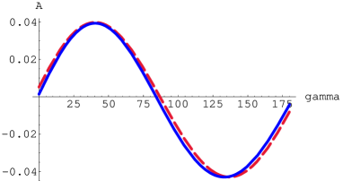
FIG. 4.: The relevant asymmetry in the decay channel $B_{s}\to K_{S}\ \pi^{+}\pi^{-}$ as a function of $\gamma$. The solid line corresponds to $\beta=24.3^{o}$ while the dashed one to $\beta=65.7^{o}$

	$\chi_{c0}+B^{*}$	$\chi_{c0}+B^{*}+B_{0}$
$Br(B^{-}\to\pi^{-}\pi^{-}\pi^{+})_{cut}$	$1.18\times 10^{-7}$	$1.06\times 10^{-7}$
$Br(B^{+}\to\pi^{-}\pi^{+}\pi^{+})_{cut}$	$1.48\times 10^{-7}$	$2.54\times 10^{-7}$
${\cal A}_{cut}$	$0.11$	$0.41$

TABLE I.: Different contributions to the branching ratio and asymmetry in the decay channel $B^{-}\to\pi^{-}\pi^{-}\pi^{+}$. Both branching ratio and asymmetry are cut off according to the rules in (18,20) and $\sin\gamma=0.82$.

REFERENCES

- [1] W. Trischuk, CDF collaboration, FERMILAB-CONF-00-044-E, CDF-PUB-BOTTOM-PUBLIC-5227; T. Affolder et al. (CDF Collaboration), hep-ex/9909003.
- [2] R. Forty, Proceedings of the International Conference on B Physics and CP Violation (BCONF99), Taipei, Taiwan, December 3-7, 1999.
- [3] Y. Gao and F. Würthwein, hep-ex/9904008; CLEO collaboration, CLEO CONF 99-13.
- [4] F. Caravaglios, F. Parodi, P. Roudeau and A. Stocchi, hep-ph/0002171.
- [5] M. Gronau and D. London, Phys. Rev. Lett. 65 3381 (1990).
- [6] A.E. Snyder and H.R. Quinn, Phys. Rev. D 48 2139 (1993); H.R. Quinn and J.P. Silva, hep-ph/0001290.
- [7] A. Deandrea, R. Gatto, M. Ladisa, G. Nardulli and P. Santorelli, Phys. Rev. D62 036001 (2000), [hep-ph/0002038].
- [8] N.G. Deshpande, G. Eilam, Xiao-Gang He and J. Trampetic, Phys. Rev. D 52 5354 (1995), [hep-ph/9503273].
- [9] G. Eilam, M. Gronau, R. R. Mendel, Phys. Rev. Lett. 74 4984 (1995).
- [10] B. Bajc, S. Fajfer, R. J. Oakes, T. N. Pham and S. Prelovsek, Phys. Lett. B447 313 (1999), [hep-ph/9809262]; S. Fajfer, R. J. Oakes and T. N. Pham Phys. Rev. D 60 054029 (1999), [hep-ph/9812313].
- [11] M. Gronau and D. Wyler, Phys. Lett. B 265 172 (1991).
- [12] P. Ball et al. (convenors): B decays at the LHC, CERN-TH/2000-101.
- [13] The BaBar Physics Book, Chapter 7, SLAC-R-504, (1998).
- [14] P. Colangelo et al., Phys. Lett. B 339, 151 (1994), [hep-ph/9406295]; V. M. Belyaev, V. M. Braun, A. Khodjamirian and R. Ruckl, Phys. Rev. D51, 6177 (1995), [hep-ph/9410280]; P. Colangelo, F. De Fazio, N. Di Bartolomeo, R. Gatto and G. Nardulli, Phys. Rev. D 52, 6422 (1995), [hep-ph/9506207]; P. Ball and V. M. Braun, Phys. Rev. D58, 094016 (1998), [hep-ph/9805422];
- [15] M. Wirbel, B. Stech and M. Bauer, Z. Phys. C29, 637 (1985); N. Isgur, D. Scora, B. Grinstein and M. B. Wise, Phys. Rev. D39, 799 (1989); P. Colangelo, F. De Fazio and G. Nardulli, Phys. Lett. B 334 175 (1994), [hep-ph/9406320]; P. Colangelo et al., Eur. Phys. J. C 8 81 (1999), [hep-ph/9809372]; M. Ladisa, G. Nardulli and P. Santorelli, Phys. Lett. B 455 283 (1999), [hep-ph/9903206].
- [16] R. Casalbuoni et al., Phys. Lett. B 299 139 (1993), [hep-ph/9211284]; Phys. Rep. 281 145 (1997), [hep-ph/9605342].
- [17] A. Deandrea, R. Gatto, G. Nardulli and A. D. Polosa, JHEP 021 9902 (1999), [hep-ph/9901266].
- [18] A.J. Buras, in ”Probing the Standard Model of Particle Interactions”, F. David and R. Gupta eds., 1998, Elsevier Science, hep-ph/9806471.
- [19] N. Cabibbo, Phys. Rev. Lett. 10 531 (1963); M. Kobayashi and T. Maskawa, Prog. Theor. Phys. 49 652 (1973).
- [20] L. Wolfenstein, Phys. Rev. Lett. 51 1945 (1983).
- [21] P. Ball, J.-M. Frère and M. Tytgat, Phys. Lett. B 365 367 (1996), [hep-ph/9508359].
- [22] R. Fleischer, Int. Jour. Mod. Phys. A 12 2459 (1997).
- [23] A. Deandrea, N. Di Bartolomeo, R. Gatto and G. Nardulli, Phys. Lett. B318, 549 (1993) [hep-ph/9308210].