Abstract

We analyze the electromagnetic form factors of the nucleon to fourth order in relativistic baryon chiral perturbation theory. We employ the recently proposed infrared regularization scheme and show that the convergence of the chiral expansion is improved as compared to the heavy fermion approach. We also discuss the inclusion of vector mesons and obtain an accurate description of all four nucleon form factors for momentum transfer squared up to $Q^{2}\simeq 0.4\,$GeV².

PACS: 12.39.Fe, 13.40.Gp, 14.20.Dh

Keywords: Nucleon electromagnetic form factors, chiral perturbation theory

1 Introduction

The electromagnetic structure of the nucleon as revealed in elastic electron–nucleon scattering is parameterized in terms of four form factors. The understanding of these form factors is of utmost importance in any theory or model of the strong interactions. Abundant data on these form factors over a large range of momentum transfer already exist, and this data base will considerably improve in the few GeV region as soon as further experiments at CEBAF will be completed and analyzed. In addition, experiments involving polarized beams and/or targets are also performed at lower energies to give better data in particular for the electric form factor of the neutron, but also for the magnetic proton and neutron ones. Such kinds of experiments have been performed or are under way at NIKHEF, MAMI, ELSA, MIT–Bates and other places. Clearly, theory has to provide a tool to interpret these data in a model–independent fashion. For small momentum transfer, this can be done in the framework of baryon chiral perturbation theory (ChPT), which is the effective field theory of the Standard Model at low energies. This will be the main topic of the present investigation.

To put our work presented here into a better perspective, let us recall what is already known from chiral perturbation theory studies of the electromagnetic form factors. Already a long time ago it was established that the isovector (Dirac and Pauli) charge radii diverge in the chiral limit of vanishing pion mass [1]. The first systematic investigation in the framework of relativistic baryon ChPT was given in [2], in particular, it was shown that the analytic structure of the one–loop representation of the isovector spectral functions is in agreement with the one deduced from unitarity (in the low energy region, that is on the left wing of the rho resonance). That approach, however, suffers from the fact that due to the use of standard dimensional regularization, the one–to–one correspondence between the expansion in loops and the one in small momenta was upset. If one considers the nucleon as a very heavy static source, a consistent power counting is possible, the so–called heavy baryon chiral perturbation theory (HBChPT). Within that approach, the electromagnetic form factors were studied in [3, 4], the latter also containing the extension to an effective field theory including the delta resonance. It was found that the chiral description already fails for values of the four–momentum transfer squared of about $Q^{2}\simeq 0.2\,$GeV². In [5], the isovector and isoscalar spectral functions were investigated in the heavy nucleon approach. It was pointed out that due to the heavy mass expansion, the analytic structure of the isovector spectral function is distorted, making the chiral expansion fail to converge in certain regions of small momentum transfer. This can be overcome in the recently proposed Lorentz–invariant formulation of [6] making use of the so–called “infrared regularization”. Being relativistic, this approach leads by construction to the correct behavior of the spectral functions in the low energy domain. Furthermore, it is expected to improve the convergence of the chiral expansion. This will be one of the main issues to be addressed here. We perform a complete one–loop analysis of the form factors, i.e. taking into account all terms up to fourth order. We will demonstrate that one can achieve a good description of the neutron charge form factor for momentum transfer squared up to about $Q^{2}=0.4\,$GeV². The other three form factors cannot be precisely reproduced by the pion cloud plus local contact terms to this order. The source of this deficiency is readily located – it stems from the contribution of vector mesons. We show how to incorporate these in a chirally symmetric manner without introducing additional free parameters (the new parameters related to the vector mesons are taken from dispersion–theoretical analyses of the form factors, see [7, 8, 9]). Within that framework, we obtain a very precise description of the large “dipole–like” form factors without destroying the good result for the neutron form factor obtained in the pure chiral expansion. It is also important to stress that the results obtained in the heavy baryon approach can be straightforwardly deduced from the framework employed here, shedding some more light on previous HBChPT results.

The manuscript is organized as follows. In section 2, some basic definitions concerning the electromagnetic form factors are collected. The one–loop representation of the nucleon form factors is given in section 3. The effective Lagrangian on which our investigation is based is briefly reviewed in subsection 3.1. In particular, infrared regularization and the treatment of loop integrals are discussed in some detail in subsection 3.2. The pertinent results based on this complete one–loop representation are presented and discussed in subsections 3.3 and 3.4. Particular emphasis is put on a direct comparison with the results obtained in heavy baryon chiral perturbation theory, which is a limiting case of the procedure employed in this manuscript. The inclusion of vector mesons in harmony with chiral symmetry is presented in section 4. We give some technicalities in subsection 4.1 and display the results for the form factors in 4.2, followed by some remarks on resonance saturation in 4.3. Concluding remarks are given in section 5. Some further technical aspects are relegated to the appendices.

2 Nucleon form factors

The structure of the nucleon (denoted by ‘$N$’) as probed by virtual photons is parameterized in terms of four form factors,

$$\langle N(p^{\prime})\,|\,{\cal J}_{\mu}\,|\,N(p)\rangle=e\,\bar{u}(p^{\prime})\,\biggl{\{}\gamma_{\mu}F_{1}^{N}(t)+\frac{i\sigma_{\mu\nu}q^{\nu}}{2m_{N}}F_{2}^{N}(t)\biggr{\}}\,u(p)\,,\quad N=p,n\,,$$ (2.1)

with $t=q_{\mu}q^{\mu}=(p^{\prime}-p)^{2}$ the invariant momentum transfer squared, ${\cal J}_{\mu}$ the isovector vector quark current, ${\cal J}_{\mu}=\bar{q}{\cal Q}\gamma_{\mu}q$ (${\cal Q}$ is the quark charge matrix), and $m_{N}$ the mean nucleon mass. In electron scattering, $t$ is negative and it is often convenient to define the positive quantity $Q^{2}=-t>0$. $F_{1}$ and $F_{2}$ are called the Dirac and the Pauli form factor, respectively, with the normalizations $F_{1}^{p}(0)=1$, $F_{1}^{n}(0)=0$, $F_{2}^{p}(0)=\kappa_{p}$ and $F_{2}^{n}(0)=\kappa_{n}$. Here, $\kappa$ denotes the anomalous magnetic moment. One also uses the electric and magnetic Sachs form factors,

$$G_{E}(t)=F_{1}(t)+\displaystyle\frac{t}{4m_{N}^{2}}F_{2}(t)\,,\quad G_{M}(t)=F_{1}(t)+F_{2}(t)\,.$$ (2.2)

In the Breit–frame, $G_{E}$ and $G_{M}$ are nothing but the Fourier–transforms of the charge and the magnetization distribution, respectively. In a relativistic framework, as it is used throughout this text, the Dirac and Pauli form factors arise if one constructs the most general nucleonic matrix element of the electromagnetic current consistent with Lorentz invariance, parity and charge conjugation. In the non–relativistic limit on the other hand, in which the nucleon can be considered as a very heavy static source, one naturally deals with the Sachs form factors. Therefore, as first stressed in [3], these arise in the heavy baryon approach to chiral perturbation theory. Since we will frequently compare our results to those obtained in that framework, we will consider both Pauli and Dirac and the Sachs form factors. For the theoretical analysis, it is advantageous to work in the isospin basis,

$$F_{i}^{s,v}(t)=F_{i}^{p}(t)\pm F_{i}^{n}(t)~{},\quad(i=1,2)~{},$$ (2.3)

since the photon has an isoscalar ($I=s$) and an isovector ($I=v$) component (and similarly for the Sachs form factors). It is important to note that the lowest hadronic states to which the isoscalar and isovector photons couple are the two and three pion systems, respectively. These are the corresponding thresholds for the absorptive parts of the isoscalar and isovector nucleon form factors.

The slope of the form factors at $t=0$ is conventionally expressed in terms of a nucleon radius $\langle r^{2}\rangle^{1/2}$,

$$F(t)=F(0)\,\biggl{(}1+\displaystyle\frac{1}{6}\langle r^{2}\rangle\,t+\ldots\biggr{)}\,$$ (2.4)

which is rooted in the non–relativistic description of the scattering process in which a point–like charged particle interacts with a given charge distribution $\rho(r)$. The mean square radius of this charge distribution is given by

$$\langle r^{2}\rangle=4\pi\,\int_{0}^{\infty}dr\,r^{2}\rho(r)=-\displaystyle\frac{6}{F(0)}\displaystyle\frac{dF(Q^{2})}{dQ^{2}}\biggr{|}_{Q^{2}=0}\,\,.$$ (2.5)

Eq. (2.5) can be used for all form factors except $G_{E}^{n}$ and $F_{1}^{n}$ which vanish at $t=0$. In these cases, one simply drops the normalization factor $1/F(0)$ and defines e.g. the neutron charge radius via

$$\langle(r_{E}^{n})^{2}\rangle\,=-6\,\displaystyle\frac{dG_{E}^{n}(Q^{2})}{dQ^{2}}\biggr{|}_{Q^{2}=0}\,\,.$$ (2.6)

It is important to note that the slopes of $G_{E}^{n}$ and $F_{1}^{n}$ are related via

$$\frac{dG_{E}^{n}(Q^{2})}{dQ^{2}}\biggr{|}_{Q^{2}=0}=\displaystyle\frac{dF_{1}^{n}(Q^{2})}{dQ^{2}}\biggr{|}_{Q^{2}=0}-\displaystyle\frac{F_{2}^{n}(0)}{4m_{N}^{2}}\,\,,$$ (2.7)

where the second term in eq. (2.7) is called the Foldy term. It gives the dominant contribution to the slope of $G_{E}^{n}$.

The large body of electron scattering data spanning momentum transfers from $Q^{2}\simeq 0$ to $Q^{2}\simeq 35\,$GeV² can be analyzed in a largely model–independent fashion using dispersion relations [7, 8, 9]. Here, we are interested in the region of small momentum transfer, $Q^{2}\leq 0.5\,$GeV². Nevertheless, since there is still some substantial scatter in the data in this range of momentum transfer, we will also use the results of the dispersive analysis for comparison to the ones obtained in the chiral expansion. A recent review on the theory of the form factors is given in [10], the status of the data as of 1999 is discussed in [11].

3 One–loop representation

3.1 Effective Lagrangian

Our starting point is an effective field theory of asymptotically observable relativistic spin–1/2 fields, the nucleons, chirally coupled to the pseudo–Goldstone bosons of QCD, the pions, and external sources (like e.g. the photon field). The theory shares the symmetries of QCD (spontaneously and explicitly broken chiral symmetry, parity, charge conjugation, time reversal invariance, and Lorentz covariance) and can be formulated in such a way as to obey systematic power counting, which will be discussed at length in the following section. External momenta and quark (pion) mass insertions are treated as small quantities in comparison to the scale of chiral symmetry breaking, $\Lambda_{\chi}\simeq 1\,$GeV. The most direct link of the effective field theory to the underlying one, QCD, comes from the analysis of the chiral Ward identities as stressed by Leutwyler [12]. Any contribution to S–matrix elements or transition currents has the form

$${\cal M}=q^{\nu}\,f\left({q\over\lambda},g\right)~{},$$ (3.1)

where $q$ is a generic symbol for any small quantity, $f$ a function of order one, $\lambda$ a regularization scale, and $g$ a collection of coupling constants. Chiral symmetry demands that the power $\nu$ is bounded from below. The expansion in increasing powers of this parameter is called the chiral expansion. At a given order, one has to consider tree as well as loop diagrams, the latter ones restoring unitarity in a perturbative fashion. The machinery to perform this is based on an effective Lagrangian, which consists of a string of terms of increasing (chiral) dimension,

$${\cal L}_{\rm eff}={\cal L}_{\pi\pi}^{(2)}+{\cal L}_{\pi N}^{(1)}+{\cal L}_{\pi N}^{(2)}+{\cal L}_{\pi N}^{(3)}+{\cal L}_{\pi N}^{(4)}+\ldots~{},$$ (3.2)

where the ellipsis denotes terms of higher order not needed here. We note that we perform a complete one–loop analysis, i.e. taking tree graphs with insertions from all terms indicated in eq. (3.2) and one–loop diagrams with insertions from ${\cal L}_{\pi N}^{(1)}$ and at most one insertion from ${\cal L}_{\pi N}^{(2)}$.

We will now consider the terms relevant to our problem (for a more detailed description, we refer the reader to [13]). The chiral effective pion Lagrangian, which to leading order contains two parameters, the pion decay constant (in the chiral limit) $F$ and the pion mass (its leading term in the quark mass expansion) $M$, is given by

$${\cal L}_{\pi\pi}^{(2)}=\frac{F^{2}}{4}\langle u_{\mu}u^{\mu}+\chi_{+}\rangle~{},$$ (3.3)

where the triplet of pion fields is collected in the SU(2) valued matrix $U(x)=u^{2}(x)$, and the chiral vielbein is related to $u$ via $u_{\mu}=i\{u^{\dagger},\nabla_{\mu}u\}$. $\nabla_{\mu}$ is the covariant derivative on the pion fields including external vector ($v_{\mu}$) and axial ($a_{\mu}$) sources, $\nabla_{\mu}U=\partial_{\mu}U-i\bigl{(}v_{\mu}+a_{\mu}\bigr{)}U+iU\bigl{(}v_{\mu}-a_{\mu}\bigr{)}$. The mass term is included in the field $\chi_{+}$ via the definitions $\chi=2B(s+i\,p)$ and $\chi_{\pm}=u^{\dagger}\chi u^{\dagger}\pm u\chi^{\dagger}u$, with $s$ and $p$ being scalar and pseudoscalar sources, respectively, the former including the quark mass matrix, $s={\cal M}+\ldots$ . Furthermore, $\langle\ldots\rangle$ denotes the trace in flavor space.

The pion–nucleon Lagrangian at leading order reads

$${\cal L}_{\pi N}^{(1)}=\bar{\Psi}\Bigl{(}iD\!\!\!\!/-m+\frac{g_{A}}{2}u\!\!\!/\gamma_{5}\Bigr{)}\Psi~{},$$ (3.4)

where the bi–spinor $\Psi$ collects the proton and neutron fields and $g_{A}$ is the axial–vector coupling constant measured in neutron $\beta$–decay, $g_{A}=1.26$. To be more precise, the nucleon mass and the axial coupling should be taken at their values in the two flavor chiral limit ($m_{u}=m_{d}=0$, $m_{s}$ fixed at its physical value). To this order, the photon field only couples to the charge of the nucleon. It resides in the chiral covariant derivative, $D_{\mu}\Psi=\partial_{\mu}\Psi+\Gamma_{\mu}\Psi$, with the chiral connection given by $\Gamma_{\mu}=\frac{1}{2}\bigl{[}u^{\dagger},\partial_{\mu}u\bigr{]}-\frac{i}{2}u^{\dagger}(v_{\mu}+a_{\mu})u-\frac{i}{2}u(v_{\mu}-a_{\mu})u^{\dagger}$.

The minimal Lagrangians at second and third order have been given in [14]. We only show the terms needed for the calculation of the form factors,

$${\cal L}_{\pi N}^{(2)} = \bar{\Psi}\,\biggl{\{}c_{1}\langle\chi_{+}\rangle-\frac{c_{2}}{8m^{2}}\Bigl{(}\langle u_{\mu}u_{\nu}\rangle\{D^{\mu},D^{\nu}\}+{\rm h.c.}\Bigr{)}+\frac{i\,c_{4}}{4}\sigma^{\mu\nu}[u_{\mu},u_{\nu}]$$ (3.5)

$$\qquad+\frac{c_{6}}{8m}\sigma^{\mu\nu}F^{+}_{\mu\nu}+\frac{c_{7}}{8m}\sigma^{\mu\nu}\langle F^{+}_{\mu\nu}\rangle\biggr{\}}\,\Psi~{},$$

$${\cal L}_{\pi N}^{(3)} = \bar{\Psi}\,\biggl{\{}\frac{i\,d_{6}}{2m}\Bigl{(}[D^{\mu},\hat{F}^{+}_{\mu\nu}]D_{\nu}+{\rm h.c.}\Bigr{)}+\frac{i\,d_{7}}{2m}\Bigl{(}[D^{\mu},\langle F^{+}_{\mu\nu}\rangle]D_{\nu}+{\rm h.c.}\Bigr{)}\biggr{\}}\,\Psi~{}.$$ (3.6)

Here, $F^{+}_{\mu\nu}=u^{\dagger}F_{\mu\nu}u+uF_{\mu\nu}u^{\dagger}$, and $F_{\mu\nu}=\partial_{\mu}A_{\nu}-\partial_{\nu}A_{\mu}$ is the conventional photon field strength tensor. Furthermore, we have adopted the notation introduced in [14] for traceless operators in SU(2), $\hat{A}=A-\frac{1}{2}\langle A\rangle$. The $c_{i}$ and $d_{i}$ are the so–called low energy constants (LECs), which encode information about the more massive states not contained in the effective field theory or other short distance effects. These parameters have to be pinned down from some data. In our case, the LECs $c_{1},\,c_{2},\,c_{4}$, which only appear in loop diagrams, can be taken from analyses of $\pi N$–scattering, whereas $c_{6},\,c_{7}$ parameterize the leading magnetic photon coupling to the nucleon, and $d_{6},\,d_{7}$ have to be fitted to the charge radii of proton and neutron.

The minimal pion–nucleon Lagrangian to fourth order has been worked out in [15]. Of the 118 terms given there, we only show the four which are of interest here,

$${\cal L}_{\pi N}^{(4)} = \bar{\Psi}\,\biggl{\{}-\frac{e_{54}}{2}\bigl{[}D^{\lambda},[D_{\lambda},\langle F^{+}_{\mu\nu}\rangle]\,]\,\sigma^{\mu\nu}-\frac{e_{74}}{2}\bigl{[}D^{\lambda},[D_{\lambda},\hat{F}^{+}_{\mu\nu}]\,]\,\sigma^{\mu\nu}$$ (3.7)

$$\qquad-\frac{e_{105}}{2}\langle F^{+}_{\mu\nu}\rangle\,\langle\chi_{+}\rangle\,\sigma^{\mu\nu}-\frac{e_{106}}{2}\hat{F}^{+}_{\mu\nu}\langle\chi_{+}\rangle\,\sigma^{\mu\nu}\biggr{\}}\,\Psi~{}.$$

Two more terms (numbered 107 and 108 respectively in [15]) only contribute when taking into account effects due to $m_{u}\neq m_{d}$. We shall disregard these in what follows. We also note that the terms $\sim e_{105},e_{106}$ only amount to a quark mass renormalization of the leading magnetic couplings $\sim c_{6},\,c_{7}$,

$$c_{6} \to \tilde{c}_{6}=c_{6}-16\,m\,M^{2}\,e_{106}~{},$$

$$c_{7} \to \tilde{c}_{7}=c_{7}-8\,m\,M^{2}\Bigl{(}2e_{105}-e_{106}\Bigr{)}~{}.$$ (3.8)

When it comes to numerical evaluation, we will just use the renormalized constants $\tilde{c}_{6}$ and $\tilde{c}_{7}$ and will not regard $e_{105}$ and $e_{106}$ as additional parameters to be fitted.

3.2 Infrared regularization

Chiral perturbation theory in the meson sector as an effective theory for weakly interacting Goldstone bosons allows for a systematic expansion of physical observables simultaneously in powers of small momenta and quark masses. For example, in the isospin limit ($m_{u}=m_{d}$) the quark mass expansion of the pion mass takes the form

$$M_{\pi}^{2}=M^{2}\biggl{\{}1-\frac{M^{2}}{32\pi^{2}F^{2}}\bar{\ell}_{3}\biggr{\}}+{\cal O}(M^{6})~{},$$ (3.9)

where the renormalized coupling $\bar{\ell}_{3}$ depends logarithmically on the quark mass, $M^{2}d\bar{\ell}_{3}/dM^{2}$ $=-1$. The infinite contribution of the pion tadpole $\sim 1/(d-4)$, see graph (a) in fig. 1, has been absorbed in the infinite part of this LEC. In this scheme, there is a consistent power counting since the only mass scale (i.e. the pion mass) vanishes in the chiral limit $m_{u}=m_{d}=0$. If one uses the same method in the nucleon case, one encounters a scale problem: for instance, if the nucleon field is treated relativistically based on standard dimensional regularization, the nucleon mass shift calculated from the self–energy diagram (see graph (b) in fig. 1) can be expressed via [2]

$$m_{N}-m=\frac{3g_{A}^{2}m^{2}}{32\pi^{2}F^{2}}\,m\,\biggl{\{}\bar{c}_{0}+\bar{c}_{1}\mu^{2}-\pi\mu^{3}-\mu^{4}\log\mu+\sum_{\nu=4}^{\infty}a_{\nu}\mu^{\nu}\biggr{\}}~{},$$ (3.10)

with $\mu=M/m$, and $\bar{c}_{0},\,\bar{c}_{1}$ are renormalized LECs (the precise relation of which to previously defined LECs is of no relevance here). This expansion is very different from the one for the pion mass, in that the nucleon mass already receives a (infinite) renormalization in the chiral limit. This difference is due to the fact that the nucleon mass does not vanish in the chiral limit and thus introduces a new mass scale apart from the one set by the quark masses. Therefore, any power of the quark masses can be generated by chiral loops in the nucleon case, whereas in the meson case a loop order corresponds to a definite number of quark mass insertions. This is the reason why one has introduced the heavy mass expansion in the nucleon case. Since in that formalism the nucleon mass is transformed from the propagator into a string of vertices with increasing powers of $1/m$, a consistent power counting can be formulated. However, this method has the disadvantage that certain types of diagrams are at odds with strictures from analyticity. The best example is the so–called triangle graph, which enters e.g. the scalar form factor or the isovector electromagnetic form factors of the nucleon (see graph (6) in fig. 2). This diagram has its threshold at $t_{0}=4M_{\pi}^{2}$ but also a singularity on the second Riemann sheet, at $t_{c}=4M_{\pi}^{2}-M_{\pi}^{4}/m_{N}^{2}=3.98M_{\pi}^{2}$, i.e. very close to threshold. To leading order in the heavy baryon approach, this singularity coalesces with the threshold and thus causes problems (a more detailed discussion can be found e.g. in [5, 16]). In a fully relativistic treatment, such constraints from analyticity are automatically fulfilled.

It was recently argued in [17] that relativistic one–loop integrals can be separated into “soft” and “hard” parts. While for the former, a similar power counting as in HBChPT applies, the contributions from the latter can be absorbed in certain LECs. In this way, one can combine the advantages of both methods. A more formal and rigorous implementation of such a program is due to Becher and Leutwyler [6]. They call their method, which we will also use here, “infrared regularization”. Any one–loop integral $H$ is split into an infrared singular and a regular part by a particular choice of Feynman parameterization. Consider first the regular part, called $R$. If one chirally expands these terms, one generates polynomials in momenta and quark masses. Consequently, to any order, $R$ can be absorbed in the LECs of the effective Lagrangian. On the other hand, the infrared singular part $I$ has the same analytical properties as the full integral $H$ in the low–energy region and its chiral expansion leads to the non–trivial momentum and quark–mass dependences of ChPT, like e.g. the chiral logarithms or fractional powers of the quark masses. It is this infrared singular part $I$ that is closely related to the heavy baryon expansion: there, the relativistic nucleon propagator is replaced by a heavy baryon propagator plus a series of $1/m$–suppressed insertions. Summing up all heavy baryon diagrams with all internal–line insertions yields the infrared singular part of the corresponding relativistic diagram.

To be specific, consider the self–energy diagram (b) of fig. 1. In $d$ dimensions, the corresponding scalar loop integral is

$$H(p^{2})=\frac{1}{i}\int\frac{d^{d}k}{(2\pi)^{d}}\frac{1}{[M^{2}-k^{2}-i\epsilon][m^{2}-(p-k)^{2}-i\epsilon]}~{}.$$ (3.11)

At threshold, $p^{2}=s_{0}=(M+m)^{2}$, this results in

$$H(s_{0})=c(d)\frac{M^{d-3}+m^{d-3}}{M+m}=I+R~{},$$ (3.12)

with $c(d)$ some constant depending on the dimensionality of space–time. The infrared singular piece $I$ is characterized by fractional powers in the pion mass and generated by loop momenta of order $M_{\pi}$. For these soft contributions, the power counting is fine. On the other hand, the infrared regular part $R$ is characterized by integer powers in the pion mass and generated by internal momenta of the order of the nucleon mass (the large mass scale). These are the terms which lead to the violation of the power counting in the standard dimensional regularization discussed above. For the self–energy integral, this splitting can be achieved in the following way:

$$H = \int\frac{d^{d}k}{(2\pi)^{d}}{1\over AB}=\int_{0}^{1}dz\int\frac{d^{d}k}{(2\pi)^{d}}{1\over[(1-z)A+zB]^{2}}$$ (3.13)

$$= \biggl{\{}\int_{0}^{\infty}-\int_{1}^{\infty}\biggr{\}}dz\int\frac{d^{d}k}{(2\pi)^{d}}{1\over[(1-z)A+zB]^{2}}=I+R~{},$$

with $A=M^{2}-k^{2}-i\epsilon$, $B=m^{2}-(p-k)^{2}-i\epsilon$. Any general one–loop diagram with arbitrary many insertions from external sources can be brought into this form by combining the propagators to a single pion– and a single nucleon–propagator. It was also shown that this procedure leads to a unique, i.e. process–independent result, in accordance with the chiral Ward identities of QCD. This is essentially based on the fact that terms with fractional versus integer powers in the pion mass must be separately chirally symmetric. Consequently, the transition from any one–loop graph $H$ to its infrared singular piece $I$ defines a symmetry–preserving regularization. However, at present it is not known how to generalize this method to higher loop orders. Also, its phenomenological consequences have not been explored in great detail so far. It is, however, expected that this approach will be applicable in a larger energy range than the heavy baryon approach.

Some remarks concerning renormalization within this scheme are in order. To leading order, the infrared singular parts coincide with the heavy baryon expansion, in particular the infinite parts of loop integrals are the same. Therefore, the $\beta$–functions for low energy constants which absorb these infinities are identical. However, infrared singular parts of relativistic loop integrals also contain infinite parts which are suppressed by powers of $\mu$, which hence cannot be absorbed as long as one only introduces counter terms to a finite order: exact renormalization only works up to the order at which one works, higher order divergences have to be removed by hand. Closely related to this problem is the one of the new mass scale $\lambda$ which one has to introduce in the process of regularization and renormalization. In dimensional regularization and related schemes, loop diagrams depend logarithmically on $\lambda$. This $\log\lambda$ dependence is compensated for by running coupling constants, the running behavior being determined by the corresponding $\beta$–functions. In the same way as the contact terms cannot consistently absorb higher order divergences, their $\beta$–functions cannot compensate for scale dependence which is suppressed by powers of $\mu$. In order to avoid this unphysical scale dependence in physical results, the authors of [6] have argued that the nucleon mass $m_{N}$ serves as a “natural” scale in a relativistic baryon ChPT loop calculation and that therefore one should set $\lambda=m_{N}$ everywhere when using the infrared regularization scheme. This was already suggested in [3] for the framework of a relativistic theory with ordinary dimensional regularization. We will follow this idea, hence in our formulae, what would actually be $\log(M_{\pi}/\lambda)$ will always be spelled out as $\log\mu$.

In the following calculation, we frequently compare our results to the equivalent heavy baryon ones. We wish to emphasize that one can always regain the heavy baryon result from the infrared regularized relativistic one by performing a strict chiral expansion of all involved loop functions. As a simple example, we again show the expansion of the nucleon mass up to third order corresponding to eq. (3.10), but this time using infrared regularization. The result is

$$m_{N}-m=-4c_{1}M^{2}+\frac{3g_{A}^{2}}{2F^{2}}mM^{2}I(m^{2})~{},$$ (3.14)

where the loop integral $I(m^{2})$ is given by

$$I(m^{2})=-\mu^{2}\biggl{(}L+\frac{1}{16\pi^{2}}\log\mu\biggr{)}+\frac{\mu}{16\pi^{2}}\biggl{\{}\frac{\mu}{2}-\sqrt{4-\mu^{2}}\arccos\biggl{(}-\frac{\mu}{2}\biggr{)}\biggr{\}}~{}.$$ (3.15)

(Definitions and results for this and all other loop functions needed in this work can be found in appendix A.) Expanding to leading order, one finds

$$I(m^{2})=-\frac{\mu}{16\pi}+{\cal O}(\mu^{2})~{},$$ (3.16)

which leads to the well–known result

$$m_{N}-m=-4c_{1}M^{2}-\frac{3g_{A}^{2}M^{3}}{32\pi F^{2}}+{\cal O}(\mu^{4})~{},$$ (3.17)

yielding a contribution non–analytic in the quark masses. As explained before, the loop function $I(m^{2})$ contains a non–leading divergence which cannot be absorbed to this order, but will be by an appropriate contact term at fourth order. The calculation of the nucleon mass to fourth order and the reduction to the heavy baryon limit is done in detail in [6].

An essential ingredient to the treatment of loop integrals as described in the previous paragraphs is the fact that higher order effects are included as compared to the “strict” chiral expansion in the heavy baryon formalism. This was justified in [6] by improved convergence properties in the low energy region, it introduces however a certain amount of arbitrariness as to which of these higher order terms to keep and which to dismiss. It is therefore mandatory to exactly describe our treatment of these terms. The philosophy in [6] was, above all, to preserve the correct relativistic analyticity properties. This was achieved by keeping the full denominators of loop integrals (and evaluating them by the infrared regularization prescription), while expanding the numerators to the desired chiral order only. In addition, e.g. crossing symmetry is to be conserved. We explore a different approach here: as we anticipate the neutron electric form factor to be highly sensitive to recoil effects, we keep all terms which occur according to the infrared regularization prescription and do not even expand the numerators of loop integrals. However, three effects involving low energy constants have to be discussed separately, all in the spirit of avoiding “artificial” higher order counterterms:

• Loop diagrams with second order insertions proportional to $c_{1}$ can easily be summarized by a shift of the “bare” nucleon mass to its renormalized value at second order, $m\rightarrow m_{N}=m-4c_{1}M_{\pi}^{2}+{\cal O}(q^{3})$. In principle, this does not occur in those loop diagrams which have insertions from other second order low energy constants. As we do not want to artificially introduce this additional LEC by discriminating between $m$ and $m_{N}$ in our formulae, we allow for this renormalization everywhere.

• As detailed in the previous section, the second order LECs $c_{6},\,c_{7}$ receive a renormalization $\sim M_{\pi}^{2}$ at fourth order. In principle, to this order only the unrenormalized $c_{i}$ appear in loop diagrams. We disregard this difference and use the same values both on tree level and for the loops.

• From the definitions of the various electromagnetic form factors, it is obvious that these are not all calculated to the same accuracy in terms of chiral orders. A calculation employing chiral Lagrangians up to and including ${\cal O}(q^{4})$ will be able to give the Dirac form factor $F_{1}$ to ${\cal O}(q^{3})$ and the Pauli form factor $F_{2}$ to ${\cal O}(q^{2})$. When combining these to the Sachs form factors $G_{E}$ and $G_{M}$, the chiral orders are “mixed”, see eq. (2.2). When we, in the following, talk about “third”/“fourth” order calculations of the various form factors, we always refer to the projections of the third/fourth order amplitude onto these observables. We truncate exactly one kind of term in this process: the ${\cal O}(q^{3})$ counterterms which enter the electric (charge) radii are really “$G_{E}$ counterterms” in the sense that they appear in $F_{1}$ and $F_{2}$ with opposite signs in order to cancel exactly in $G_{M}$. In addition, there are, at ${\cal O}(q^{4})$, $F_{2}$ counterterms fixing the magnetic radii. Therefore, $G_{E}$ receives $q^{4}$ counterterms inherited from $({q^{2}}/{4m^{2}})F_{2}$. As a genuine polynomial contribution of this kind only appears in an ${\cal O}(q^{5})$ calculation, we drop these terms in $G_{E}$.

3.3 Chiral expansion of the nucleon form factors

The chiral expansion of a form factor $F$ (being a genuine symbol for any of the four electromagnetic nucleon form factors) consists of two contributions, tree and loop graphs. The tree graphs comprise that of lowest order with a fixed coupling (the nucleon charge) as well as counterterms from the second, third, and fourth order Lagrangians. As one–loop graphs, we have both those with just lowest order couplings and those with exactly one insertion from ${\cal L}_{\pi N}^{(2)}$. The pertinent tree and loop graphs are depicted in fig. 2 (we have not shown the diagrams leading to wave function renormalization). The first four of these comprise the tree graphs with insertions up to dimension four, and diagrams (5) to (9) ((10) to (12)) are the third (fourth) order loop graphs. Consequently, any form factor can be written as

$$F(t)=F^{\rm tree}(t)+F^{\rm loop}(t)~{}.$$ (3.18)

In appendix B, we have listed the contributions to the Dirac and Pauli form factors from the various diagrams, including the nucleon Z–factor. This allows to reconstruct the pertinent expressions for $F_{1,2}^{p,n}$ in a straightforward manner. We refrain from giving the complete expressions here. The corresponding Sachs form factors $G_{E,M}^{p,n}$ are obtained by use of eq. (2.2) under the restrictions discussed in the preceding section. We only show the explicit formulae for the magnetic moments, the electric and the magnetic radii (in terms of renormalized, i.e. physical, masses and coupling constants). The magnetic moments read

$$\kappa^{v} = \tilde{c}_{6}^{r}$$ (3.19)

$$- \frac{\mu^{2}g_{A}^{2}m_{N}^{2}}{(4\pi F_{\pi})^{2}}\biggl{\{}\frac{3}{2}\mu^{2}+\biggl{(}2-\frac{\mu^{2}}{4}\biggr{)}\,c_{6}$$

$$\qquad+\,\frac{\arccos(-\frac{\mu}{2})}{\mu\sqrt{4-\mu^{2}}}\biggl{[}2\Bigl{(}8-13\mu^{2}+3\mu^{4}\Bigr{)}-\mu^{2}\biggl{(}8-\frac{5}{2}\mu^{2}\biggr{)}\,c_{6}\biggr{]}$$

$$\qquad+\,\biggl{[}2\Bigl{(}7-3\mu^{2}\Bigr{)}+\biggl{(}4-\frac{5}{2}\mu^{2}\biggr{)}\,c_{6}\biggr{]}\log\mu\biggr{\}}$$

$$+ \frac{\mu^{2}m_{N}^{2}}{(4\pi F_{\pi})^{2}}\biggl{\{}\frac{3}{4}\mu^{2}m_{N}\,c_{2}-\Bigl{(}3\mu^{2}m_{N}\,c_{2}-8m_{N}\,c_{4}+2c_{6}\Bigr{)}\log\mu\biggr{\}}~{},$$

$$\kappa^{s} = \tilde{c}_{6}^{r}+2\tilde{c}_{7}^{r}$$ (3.20)

$$- \frac{3\mu^{2}g_{A}^{2}m_{N}^{2}}{(4\pi F_{\pi})^{2}}\biggl{\{}\frac{\mu^{2}}{4}\Bigl{(}2+c_{6}+2c_{7}\Bigr{)}$$

$$\qquad-\,\frac{\mu\arccos(-\frac{\mu}{2})}{\sqrt{4-\mu^{2}}}\biggl{[}2\Bigl{(}3-\mu^{2}\Bigr{)}+\biggl{(}4-\frac{3}{2}\mu^{2}\biggr{)}\Bigl{(}c_{6}+2c_{7}\Bigr{)}\biggr{]}$$

$$\qquad+\,\biggl{[}2\Bigl{(}1-\mu^{2}\Bigr{)}+\Bigl{(}2-\frac{3}{2}\mu^{2}\Bigr{)}\Bigl{(}c_{6}+2c_{7}\Bigr{)}\biggr{]}\log\mu\biggr{\}}$$

$$+ \frac{3\mu^{4}m_{N}^{3}\,c_{2}}{(4\pi F_{\pi})^{2}}\biggl{(}\frac{1}{4}-\log\mu\biggr{)}~{},$$

with $\mu=M_{\pi}/m_{N}\simeq 1/7$. Note that the magnetic moments are finite in the chiral limit. We remind the reader of the definitions of $\tilde{c}_{6}$ and $\tilde{c}_{7}$ in eq. (3.8). We have distinguished between the renormalized and the unrenormalized LECs (at tree level and in loop contributions, respectively) only for reasons of formal exactitude, and will disregard this difference from now on. Note however that, in contrast to $c_{6},\,c_{7}$, these renormalized LECs inherit infinite parts from $e_{105},\,e_{106}$ which are needed in order to remove the leading order divergences in the magnetic moments (as explained in section 3.2). Their poles in $(d-4)$ are determined by the corresponding $\beta$–functions,

$$\beta_{e_{105}} = -\frac{3g_{A}^{2}}{16m_{N}}\Bigl{(}1+c_{6}+2c_{7}\Bigr{)}~{},$$ (3.21)

$$\beta_{e_{106}} = -\frac{1}{8m_{N}}\Bigl{[}7g_{A}^{2}-4m_{N}c_{4}+(1+2g_{A}^{2})c_{6}\Bigr{]}~{}.$$ (3.22)

$\tilde{c}_{6}^{r},\,\tilde{c}_{7}^{r}$ in eqs. (3.19), (3.20) denote the finite LECs, i.e. with the poles subtracted. Next, the charge radii can be brought into the form

$$(r_{E}^{v})^{2} = -12\,d_{6}^{r}+\frac{3\,\kappa^{v}}{2m_{N}^{2}}$$ (3.23)

$$- \frac{g_{A}^{2}}{(4\pi F_{\pi})^{2}}\biggl{\{}7-8\mu^{2}-\frac{3}{4}\mu^{4}\Bigl{(}1-c_{6}\Bigr{)}$$

$$\qquad-\,\frac{\mu\arccos(-\frac{\mu}{2})}{\sqrt{4-\mu^{2}}}\Bigl{[}70-74\mu^{2}+15\mu^{4}+3\mu^{2}\Bigl{(}3-\mu^{2}\Bigr{)}c_{6}\Bigr{]}$$

$$\qquad+\,\Bigl{[}10-44\mu^{2}+15\mu^{4}+3\mu^{2}\Bigl{(}1-\mu^{2}\Bigr{)}c_{6}\Bigr{]}\log\mu\biggr{\}}$$

$$- \frac{1}{(4\pi F_{\pi})^{2}}\Bigl{(}1+2\log\mu\Bigr{)}~{},$$

$$(r_{E}^{s})^{2} = -24\,d_{7}+\frac{3\,\kappa^{s}}{2m_{N}^{2}}$$ (3.24)

$$+ \frac{3\mu^{2}g_{A}^{2}}{(4\pi F_{\pi})^{2}}\biggl{\{}\frac{2}{4-\mu^{2}}+\frac{\mu^{2}}{4}\Bigl{[}1+3\Bigl{(}c_{6}+2c_{7}\Bigr{)}\Bigr{]}$$

$$\qquad-\,\frac{\mu\arccos(-\frac{\mu}{2})}{(4-\mu^{2})^{3/2}}\Bigl{[}54-34\mu^{2}+5\mu^{4}+3\Bigl{(}12-7\mu^{2}+\mu^{4}\Bigr{)}\Bigl{(}c_{6}+2c_{7}\Bigr{)}\Bigr{]}$$

$$\qquad+\,\Bigl{[}4-5\mu^{2}+3\Bigl{(}1-\mu^{2}\Bigr{)}\Bigl{(}c_{6}+2c_{7}\Bigr{)}\Bigr{]}\log\mu\biggr{\}}~{}.$$

The isovector charge radius diverges logarithmically in the chiral limit, while the isoscalar one is finite. $d_{6}^{r}$ denotes the renormalized LEC $d_{6}$, i.e. without the infinite part that removes the leading order divergence in the isovector electric form factor, the corresponding $\beta$–function being given by [18, 14]

$$\beta_{d_{6}}=-\frac{1+5g_{A}^{2}}{6}~{}.$$ (3.25)

The LEC $d_{7}$ entering the isoscalar radius is, in contrast, finite. Finally, the magnetic radii are given by

$$\mu^{v}(r_{M}^{v})^{2} = 24\,m_{N}\,e_{74}^{r}$$ (3.26)

$$+ \frac{g_{A}^{2}}{(4\pi F_{\pi})^{2}}\biggl{\{}\frac{1}{4(4-\mu^{2})}\Bigl{[}112-36\mu^{2}-8\mu^{4}+3\mu^{6}-\mu^{2}\Bigl{(}8-8\mu^{2}+\mu^{4}\Bigr{)}\,c_{6}\Bigr{]}$$

$$\qquad+\,\frac{\arccos(-\frac{\mu}{2})}{\mu(4-\mu^{2})^{3/2}}\Bigl{[}32-152\mu^{2}+126\mu^{4}-34\mu^{6}+3\mu^{8}-\mu^{4}\Bigl{(}6-6\mu^{2}+\mu^{4}\Bigr{)}\,c_{6}\Bigr{]}$$

$$\qquad+\,\Bigl{[}14-16\mu^{2}+3\mu^{4}\Bigl{(}3-c_{6}\Bigr{)}\Bigr{]}\log\mu\biggr{\}}$$

$$- \frac{1}{(4\pi F_{\pi})^{2}}\Bigl{(}1+2\log\mu\Bigr{)}\Bigl{(}1+4m_{N}\,c_{4}\Bigr{)}~{},$$

$$\mu^{s}(r_{M}^{s})^{2} = 48\,m_{N}\,e_{54}$$ (3.27)

$$- \frac{3\mu^{2}g_{A}^{2}}{(4\pi F_{\pi})^{2}}\biggl{\{}\frac{8-8\mu^{2}+\mu^{4}}{4(4-\mu^{2})}+\frac{\mu\arccos(-\frac{\mu}{2})}{(4-\mu^{2})^{3/2}}\Bigl{(}6-6\mu^{2}+\mu^{4}\Bigr{)}+\mu^{2}\log\mu\biggr{\}}$$

$$\qquad\qquad\times\Bigl{(}1+c_{6}+2c_{7}\Bigr{)}~{},$$

where, again, $e_{74}^{r}$ has the infinite part, which is given by

$$\beta_{e_{74}}=-\frac{1}{3m_{N}}\Bigl{(}3g_{A}^{2}-m_{N}c_{4}\Bigr{)}~{},$$ (3.28)

subtracted, while $e_{54}$ in the isoscalar radius (in analogy to $d_{7}$ for the electric isoscalar radius) is finite. The isovector magnetic radius explodes like $1/M_{\pi}$ as the pion mass goes to zero, while, again, the isoscalar radius is finite in the chiral limit. These chiral limit results are to be expected because the Sachs form factors inherit the well known chiral singularities of the isovector Dirac and Pauli form factors, more precisely, the corresponding radii diverge in the chiral limit as

$$(r_{1}^{v})^{2} = -{10g_{A}^{2}+2\over(4\pi F_{\pi})^{2}}\,\log\frac{M_{\pi}}{m_{N}}+\ldots~{},$$

$$(r_{2}^{v})^{2} = {g_{A}^{2}m_{N}\over 8\pi F_{\pi}^{2}\kappa_{v}M_{\pi}}+\ldots~{},$$ (3.29)

where the ellipsis denotes subleading terms as the pion mass vanishes. This dominant pion loop effect in the nucleon form factors has already been established a long time ago [1]. It can also be expected on physical grounds: the pion cloud, which is Yukawa suppressed for finite pion mass, becomes long–ranged in the chiral limit leading to a divergent contribution. Such phenomena are also observed in two–photon observables like e.g. the electromagnetic polarizabilities of the nucleon. Also, as a consequence of analyticity, in the heavy baryon approach (i.e. in a strict chiral expansion) the isoscalar form factors are, to one–loop order, given simply by a polynomial subsuming tree and counterterm contributions. There are, however, isoscalar loop effects as higher order corrections, as is obvious from the above. These stem from the diagrams with the photon coupling to the nucleons (see graphs (5) and (10) in fig. 2), which only yield constant terms needed for renormalization in HBChPT, but also contain higher order $t$–dependent terms. As the spectral function corresponding to these diagrams only starts to contribute for $t\geq 4m_{N}^{2}$, these $t$–dependent terms (in the real part) are highly suppressed.

In section 3.2, we already mentioned the marked difference in the threshold behavior of the isovector spectral functions in the relativistic and the heavy baryon approach. We only quote the results for the threshold behavior here and relegate the full results to appendix C. Note that these have already been given in the literature, the relativistic results to third order in [2], the additional fourth order contribution as well as the heavy baryon expansions in [5]. We reemphasize that the imaginary parts in the infrared regularization approach do not differ from those in a fully relativistic calculation. For Im$\,F_{1}^{v}(t)$, the relativistic threshold expansion is given by

$${\rm Im}\,F_{1}^{v}(t)=\frac{1}{192\pi F_{\pi}^{2}\,M_{\pi}^{3}}\biggl{\{}g_{A}^{2}\Bigl{(}4m_{N}^{2}-M_{\pi}^{2}\Bigr{)}+M_{\pi}^{2}\biggr{\}}\,(t-4M_{\pi}^{2})^{3/2}+{\cal O}\Bigl{(}(t-4M_{\pi}^{2})^{5/2}\Bigr{)}~{},$$ (3.30)

and for Im$\,F_{2}^{v}(t)$, one finds

$${\rm Im}\,F_{2}^{v}(t)=\frac{m_{N}\,c_{4}}{48\pi F_{\pi}^{2}\,M_{\pi}}\,(t-4M_{\pi}^{2})^{3/2}+{\cal O}\Bigl{(}(t-4M_{\pi}^{2})^{5/2}\Bigr{)}~{}.$$ (3.31)

In the heavy baryon scheme, however, the heavy mass expansion yields the expressions

$${\rm Im}\,F_{1}^{v}(t) = \frac{g_{A}^{2}}{96\pi F_{\pi}^{2}}\biggl{\{}\sqrt{1-\frac{4M_{\pi}^{2}}{t}}\Bigl{(}5t-8M_{\pi}^{2}\Bigr{)}-\frac{3\pi}{4m_{N}}\,\frac{3t^{2}-12M_{\pi}^{2}t+8M_{\pi}^{4}}{t^{1/2}}\biggr{\}}$$ (3.32)

$$+\,\frac{1}{96\pi F_{\pi}^{2}}\,\frac{(t-4M_{\pi}^{2})^{3/2}}{t^{1/2}}\,+{\cal O}(q^{4})~{},$$

$${\rm Im}\,F_{2}^{v}(t) = \frac{g_{A}^{2}\,m_{N}}{32F_{\pi}^{2}}\biggl{\{}\frac{t-4M_{\pi}^{2}}{t^{1/2}}-\frac{4}{\pi m_{N}}\,\sqrt{1-\frac{4M_{\pi}^{2}}{t}}\,\Bigl{(}t-2M_{\pi}^{2}\Bigr{)}\biggr{\}}$$ (3.33)

$$+\,\frac{m_{N}\,c_{4}}{24\pi F_{\pi}^{2}}\,\frac{(t-4M_{\pi}^{2})^{3/2}}{t^{1/2}}\,+{\cal O}(q^{3})~{},$$

which evidently violate the required threshold behavior ${\rm Im}\,F_{i}^{v}(t)\sim(t-4M_{\pi}^{2})^{3/2}$ as pointed out in [5]. As remarked before, this is due to the fact that the two–pion threshold and the singularity on the second Riemann sheet, inherited from the $\pi\pi\to\bar{N}N$ partial waves, coalesce in the heavy baryon limit. In contrast, the relativistic approach of course yields the correct analytical structures (for a more pedestrian discussion of this point, see e.g. [16]).

3.4 Results and discussion

First, we must fix parameters. We use $F_{\pi}=92.4\,$MeV, $M_{\pi}=139.57\,$MeV, $g_{A}=1.26$, and $m_{N}=(m_{p}+m_{n})/2=938.92\,$MeV. The LECs $c_{2}$ and $c_{4}$ are taken from the analysis of pion–nucleon scattering [14, 19], $c_{2}=3.2\,$GeV^-1 and $c_{4}=3.4\,$GeV^-1. The LECs $c_{6}$ and $c_{7}$ can be pinned down from the well known magnetic moments of proton and neutron. The remaining two “electric” ($d_{6},\,d_{7})$ and two “magnetic” LECs ($e_{54},\,e_{74})$ are determined from the electric and magnetic radii as given by the dispersion theoretical analysis of [8], these values are $r_{E}^{p}=0.847\,$fm, $(r_{E}^{n})^{2}=-0.113\,$fm², $r_{M}^{p}=0.836\,$fm and $r_{M}^{n}=0.889\,$fm. We note that the long standing discrepancy of the proton charge radius determination from electron–proton scattering [20] and Lamb shift measurements [21] has been resolved, converging to a value of $r_{E}^{p}=(0.88\pm 0.01)\,$fm. We do not use this value here because so far no dispersion theoretical analysis exists using this novel information.

As already stated, the Dirac and Pauli form factors are the natural quantities in any relativistic approach like the one used here. However, for easier comparison to existing heavy baryon calculations and to the low energy data, which are often presented in terms of Sachs form factors, we will discuss these in detail.

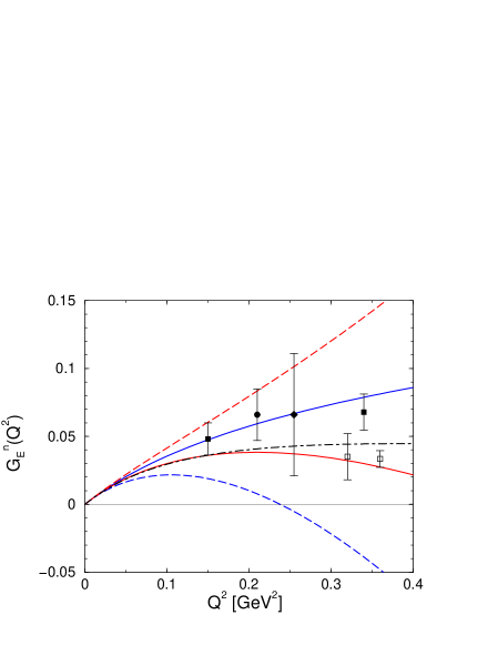
Figure 3: The neutron electric form factor in relativistic baryon chiral perturbation theory (solid lines) to third (blue curve) and fourth (red curve) order. For comparison, the results of the heavy baryon approach are also shown (blue/red dashed line: third/fourth order). All LECs are determined by a fit to the neutron charge radius measured in neutron–atom scattering. Also given is the result of the dispersion theoretical analysis (black dot–dashed curve). The data are from [22].

First we discuss the neutron charge form factor, as shown in fig. 3. The third and fourth order results compare well to the dispersion theoretical analysis and the trend of the novel data up to $Q^{2}=0.4\,$GeV². The latter have been obtained using tensor polarized deuterium, polarized ³He and polarization transfer on deuterium [22]. Although it seems that the third order curve meets the novel data even better, we observe that the fourth order one is basically identical to the dispersion theoretical fit up to $Q^{2}=0.2\,$GeV². Also given in that figure are the heavy baryon results to third [4] and fourth [23] order. These curves can easily be obtained from our analysis by performing the large mass expansion as explained before. Clearly, neither of these two curves is in acceptable agreement with the data, and, what is more, there is no sign of convergence so far. The resummation of the $1/m$ terms in the relativistic approach vastly improves the convergence of the chiral representation. This sensitivity of the neutron charge form factor to such recoil corrections was already anticipated in [24]. We remark however that the only fourth order contributions to the electric form factors in the heavy baryon approach are $1/m$–corrections to third order diagrams, in other words, the full fourth order heavy baryon result for these can already be obtained from expanding the third order relativistic one. Therefore, the difference that does show up between the relativistic third and fourth order curves is really, in terms of strict chiral power counting, of higher order and hence (comparably) small.

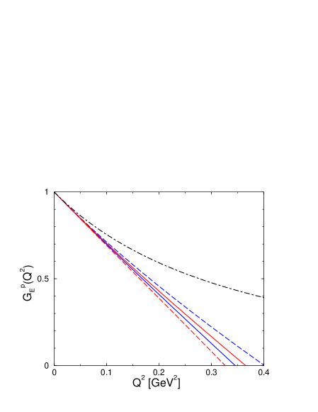
Figure 4: The proton electric form factor in relativistic baryon chiral perturbation theory (solid lines) to third (blue curve) and fourth (red curve) order. For comparison, the results of the heavy baryon approach are also shown (blue/red dashed line: third/fourth order). All LECs are determined by a fit to the proton charge radius as given by the dispersion theoretical result (black dot–dashed curve).

Consider the proton electric form factor next, shown in fig. 4. As in the neutron case, the third and fourth order curves are very close (where, however, the remarks made about the reasons for the smallness of this difference apply equally here), but here essentially show the linear behavior from the term proportional to the charge radius. Compared to the dispersion theoretical result (which describes the data very well in this range of momentum transfer), there is clearly not enough curvature. Polynomial terms of order $t^{2}$ (and higher) are not included up to fourth order, and the curvature coming solely from loop functions in the one–loop approximation is obviously not sufficient. Fig. 4 also displays the results of the third [3, 4] and fourth [23] order heavy baryon calculation. While the general trend of the heavy baryon results is similar to what is obtained in the relativistic approach (far too small curvature to meet the data), we note that, while there is at least a slight improvement from the third to the fourth order relativistic calculation, the description visibly worsens for the fourth order heavy baryon result, as compared to the third order one.

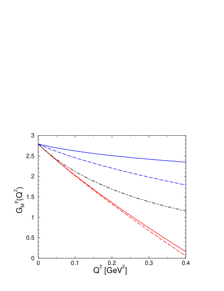
Figure 5: The proton magnetic form factor in relativistic baryon chiral perturbation theory (solid lines) to third (blue curve) and fourth (red curve) order. For comparison, the results of the heavy baryon approach are also shown (blue/red dashed line: third/fourth order). The third (fourth) order LECs are determined by a fit to the proton magnetic moment (radius). Also given is the dispersion theoretical result (black dot–dashed curve).

We now turn to the magnetic form factors of proton and neutron as shown in figs. 5, 6. The qualitative behavior of the different curves is very similar for both of them: To third order, the momentum dependence is given parameter–free because the LECs at this order only affect the normalization. We see that the $1/m$ corrections present in our approach visibly worsen the prediction obtained previously in the heavy baryon limit. That result is based on the leading chiral singularities given in eq. (3.3) because to this order, the corresponding isoscalar form factor is simply constant. We conclude that the recoil corrections are rather large and that the leading chiral limit behavior is not a good approximation for the Goldstone boson contribution to the magnetic radii in the case of finite pion masses. At fourth order, due to the presence of the counterterms from ${\cal L}_{\pi N}^{(4)}$, the radius can be fixed at its empirical value. Consequently, the full relativistic result and its heavy baryon limit are not very different any more. The absence of curvature terms of order $t^{2}$ (and higher) is clearly visible in figs. 5, 6.

The physics underlying this deficiency will be addressed in section 4. Only a uniformly reliable description for all four form factors is acceptable, and hence it is absolutely necessary to understand what is missing in the three dipole–shaped form factors: with large corrections for these, one might expect large corrections also for the neutron charge form factor, such that its very good description presented here might turn out to be only accidental. In the following, we shall show that this is indeed not the case.

4 Inclusion of vector mesons

It is well established that the vector mesons contribute significantly to the nucleon form factors. For example, extended unitarity allows one to reconstruct the isovector spectral functions [25] below $t\simeq 1\,$GeV² from the pion form factor and the analytically continued $\pi\pi\to\bar{N}N$ isovector partial wave amplitudes. Besides the important contribution of the two–pion continuum, the $\rho$ meson clearly shows up. Similarly, in the isoscalar channel, the $\omega$ and the $\phi$ dominate the spectral function at low positive $t$. All these effects are clearly visible in dispersion theoretical analyses of the nucleon form factors, see [7, 8, 9]. In the chiral expansion performed in the preceding sections, such effects are included in the low energy constants. This follows directly from the low momentum expansion of any vector meson propagator (for simplicity, we do not show the explicit Lorentz structures),

$$\frac{1}{1-{t}/{M_{V}^{2}}}=1+\displaystyle\frac{t}{M_{V}^{2}}+\displaystyle\frac{t^{2}}{M_{V}^{4}}+{\cal O}(t^{3})~{}.$$ (4.1)

In a fourth order chiral analysis as presented here, one is sensitive up to the terms linear in $t$, which contribute to the various electromagnetic radii. Stated differently, any vector meson contribution is hidden in the fit values of the various LECs. As we discussed before, the curvature effects on the electric and magnetic form factor of the proton as well as the magnetic neutron form factor are much too small. This can be cured in two ways. One could either attempt a higher order analysis or include vector mesons dynamically. While the first approach would be more systematic, we choose here the second, for various reasons. With explicit vector mesons (VM), we not only account for all terms in the expansion eq. (4.1) but also do not introduce any new unknown parameter. This can be understood as follows: adding the vector mesons in a chirally symmetric manner and retaining the corresponding dimension two, three and four counterterms, any LEC $\alpha_{i}$ takes the form

$$\alpha_{i}\,\to\,\hat{\alpha}_{i}\,+\,{\rm vector~{}meson}\!-\!{\rm contribution}~{},$$ (4.2)

where the remainder $\hat{\alpha}_{i}$ parameterizes the physics not related to the explicitly included vector meson contribution. For such a decomposition to make sense, the scale dependent LECs should be taken at $\lambda=M_{V}$. Since in the infrared regularization procedure, the nucleon mass is taken to be the intrinsic scale for all loop integrals as described in section 3.2, here we neglect scale mismatch due to $M_{V}\neq m_{N}$ (which is probably justified because of $\log(m_{N}/M_{\rho})\approx 0.2$). The vector meson propagator generates a whole string of higher order terms, hopefully resumming the most important contributions not included at fourth order. The parameters appearing in the vector meson contributions will be taken from existing dispersive analyses of the nucleon electromagnetic form factors. We therefore only need to refit the low energy constants $\hat{\alpha}_{i}$. This also allows to study the concept of resonance saturation. It was already shown in [26] that the numerical values of the dimension two LECs can be understood from s–channel baryon and t–channel meson resonance excitations, in particular from the $\Delta(1232)$ and the $\rho$. In the case at hand, we can investigate this concept for the LECs $c_{6}$, $c_{7}$, $d_{6}$, $d_{7}$, $e_{54}$, and $e_{74}$. It was already noted in [26] that $c_{6}$ and $c_{7}$ are largely saturated by vector meson contributions.

4.1 Chiral Lagrangians including vector mesons

We employ the tensor field representation of spin-1 fields as advocated in [27], i.e. the vector mesons are written in terms of antisymmetric tensor fields

$$W_{\mu\nu}=-W_{\nu\mu}$$ (4.3)

with the three degrees of freedom $W_{ij}$ ($i,j=1,2,3$) frozen out. This representation is most natural for constructing chirally invariant couplings of vector mesons to pions and photons because no particular dynamical character of the vector mesons is assumed (in contrast e.g. to the massive Yang–Mills or hidden symmetry approaches as reviewed in [28, 29].) In this section, we temporarily switch to SU(3) chiral Lagrangians, because the $\phi$ meson contributes to the isoscalar form factors. The free Lagrangian then takes the form

$${\cal L}_{V}=-\frac{1}{2}\partial^{\mu}W^{a}_{\mu\nu}\partial_{\rho}W^{\rho\nu,a}+\frac{M_{V}^{2}}{4}W^{a}_{\mu\nu}W^{\mu\nu,a}~{},$$ (4.4)

where

$$W_{\mu\nu}=\left(\begin{array}[]{ccc}\frac{\rho^{0}}{\sqrt{2}}+\frac{\omega}{\sqrt{2}}&\rho^{+}&K^{*+}\\ \rho^{-}&-\frac{\rho^{0}}{\sqrt{2}}+\frac{\omega}{\sqrt{2}}&K^{*0}\\ K^{*-}&\overline{K}^{*0}&-\phi\end{array}\right)_{\mu\nu}~{}.$$ (4.5)

Here, we have written the vector meson matrix in terms of physical particles, assuming ideal $\phi$–$\omega$ mixing. From eq. (4.4), one easily derives the vector meson propagator as given in [30],

$$G_{\mu\nu,\rho\sigma}(x,y) = \langle 0|T\{W_{\mu\nu}(x),W_{\rho\sigma}(y)\}|0\rangle$$ (4.6)

$$= \frac{i}{M_{V}^{2}}\int\frac{d^{4}k}{(2\pi)^{4}}\frac{e^{ik\cdot(x-y)}}{M_{V}^{2}-k^{2}-i\epsilon}$$

$$\times\Bigl{[}g_{\mu\rho}g_{\nu\sigma}(M_{V}^{2}-k^{2})+g_{\mu\rho}k_{\nu}k_{\sigma}-g_{\mu\sigma}k_{\nu}k_{\rho}-(\mu\leftrightarrow\nu)\Bigr{]}~{}.$$

According to [31], the lowest order interaction with Goldstone boson fields as well as external vector and axial–vector sources can be written as

$${\cal L}_{W}=\frac{1}{2\sqrt{2}}\Bigl{(}F_{V}\langle W^{\mu\nu}F^{+}_{\mu\nu}\rangle+iG_{V}\langle W^{\mu\nu}[u_{\mu},u_{\nu}]\rangle\Bigr{)}~{},$$ (4.7)

where the couplings $G_{V}$ and $F_{V}$ can e.g. be determined from the decay widths $\rho\to\pi\pi$ and $\rho\to e^{+}e^{-}$. Following [30], the lowest order couplings of massive spin–1 fields to baryons can be written in terms of a chirally invariant Lagrangian as

$${\cal L}_{\phi BW} = R_{D/F}\,\langle\bar{B}\sigma^{\mu\nu}(W_{\mu\nu},B)_{\pm}\rangle\,+\,R_{S}\,\langle\bar{B}\sigma^{\mu\nu}B\rangle\,\langle W_{\mu\nu}\rangle$$ (4.8)

$$+S_{D/F}\,\langle\bar{B}\gamma^{\mu}([D^{\nu},W_{\mu\nu}],B)_{\pm}\rangle\,+\,S_{S}\,\langle\bar{B}\gamma^{\mu}B\rangle\,\langle[D^{\nu},W_{\mu\nu}]\rangle$$

$$+U_{D/F}\,\langle\bar{B}\sigma^{\lambda\nu}(W_{\mu\nu},[D_{\lambda},[D^{\mu},B]])_{\pm}\rangle\,+\,U_{S}\,\langle\bar{B}\sigma^{\lambda\nu}[D_{\lambda},[D^{\mu},B]]\rangle\langle W_{\mu\nu}\rangle~{},$$

where, as usually in SU(3), the index $D$ refers to the anticommutator $(A,B)_{+}=\{A,B\}$, while the index $F$ accompanies the commutator $(A,B)_{-}=[A,B]$. In addition, we introduced singlet couplings with indices $S$. These coupling constants are related to the ones used in the Lagrangian of the standard vector representation of the $\rho$,

$${\cal L}_{\rho N}=\frac{1}{2}g_{\rho NN}\bar{\Psi}\Bigl{\{}\gamma^{\mu}\boldsymbol{\rho}_{\mu}\!\cdot\!\boldsymbol{\tau}-\frac{\kappa_{\rho}}{2m_{N}}\sigma^{\mu\nu}\partial_{\nu}\boldsymbol{\rho}_{\mu}\!\cdot\!\boldsymbol{\tau}\Bigr{\}}\Psi~{},$$ (4.9)

by

$$g_{\rho NN} = \frac{M_{V}}{\sqrt{2}}\Bigl{(}m_{N}(U_{D}+U_{F})-2(S_{D}+S_{F})\Bigr{)}~{},$$ (4.10)

$$g_{\rho NN}\,\kappa_{\rho} = -\frac{4\sqrt{2}m_{N}}{M_{V}}(R_{D}+R_{F})~{}.$$ (4.11)

In analogy, one finds for the $\omega$ and $\phi$ couplings

$$g_{\omega NN} = \frac{M_{V}}{\sqrt{2}}\Bigl{(}m_{N}(U_{D}+U_{F}+2U_{S})-2(S_{D}+S_{F}+2S_{S})\Bigr{)}~{},$$ (4.12)

$$g_{\omega NN}\,\kappa_{\omega} = -\frac{4\sqrt{2}m_{N}}{M_{V}}(R_{D}+R_{F}+2R_{S})~{},$$ (4.13)

$$g_{\phi NN} = -M_{V}\Bigl{(}m_{N}(U_{D}-U_{F}+U_{S})-2(S_{D}-S_{F}+S_{S})\Bigr{)}~{},$$ (4.14)

$$g_{\phi NN}\,\kappa_{\phi} = \frac{8m_{N}}{M_{V}}(R_{D}-R_{F}+R_{S})~{}.$$ (4.15)

In [30], one additional term (proportional to new couplings $T_{D/F}$) of higher order in derivatives was introduced,

$${\cal L}^{\prime}_{\phi BW}=T_{D/F}\,\langle\bar{B}\gamma^{\mu}([D_{\lambda},W_{\mu\nu}],[D^{\lambda},[D^{\nu},B]])_{\pm}\rangle\,+\,T_{S}\,\langle\bar{B}\gamma^{\mu}[D^{\lambda},[D^{\nu},B]]\rangle\,\langle[D_{\lambda},W_{\mu\nu}]\rangle~{},$$ (4.16)

which was subsequently shown to contribute to the electric form factors as a term ${\cal O}(q^{4})$, therefore beyond the order to which we are working here; the authors of [30] however left out a term

$${\cal L}^{\prime\prime}_{\phi BW}=V_{D/F}\,\langle\bar{B}\sigma^{\nu\lambda}([D_{\lambda},[D^{\mu},W_{\mu\nu}]],B)_{\pm}\rangle\,+\,V_{S}\,\langle\bar{B}\sigma^{\nu\lambda}B\rangle\,\langle[D_{\lambda},[D^{\mu},W_{\mu\nu}]]\rangle$$ (4.17)

which enters the magnetic radius, i.e. contributes a term ${\cal O}(q^{2})$ to the magnetic form factors and hence should be considered in a ${\cal O}(q^{4})$ calculation. However, as nothing is known from elsewhere about such couplings, we shall not introduce these here. Note that, via the $q^{2}$–expansion of the resonance pole, the contributions to the magnetic moments stemming from the $R_{D/F/S}$ terms do of course induce additional $q^{2}$–dependence in the magnetic form factors.

There is no generalization of chiral perturbation theory which fully includes the effects of vector mesons as intermediate states to arbitrary loop orders. As the masses of the vector mesons do not vanish in the chiral limit, they introduce a new mass scale which, when appearing inside loop integrals, potentially spoils chiral power counting in a similar manner as the nucleon mass in a “naive” relativistic baryon ChPT approach. In analogy to the heavy fermion theories, “heavy meson effective theory” has been used to investigate vector meson properties like masses and decay constants when coupling these to Goldstone bosons in a chirally invariant fashion (see [33] or for some special processes [34]). This approach does not work with the heavy particle number not conserved as in processes with these resonances being virtual intermediate states. However, these difficulties do not arise as long as there is no loop integration over intermediate vector meson momenta. Indeed, to the order we are working here, we can even set up a “power counting scheme” for diagrams including vector mesons which allows to calculate corrections to the simple tree diagrams (where the photon couples to the nucleon via an intermediate vector meson). We count

1. the couplings of vector mesons to the photon and of the $\rho$ to two pions as ${\cal O}(q^{2})$ (see eq. (4.7) and the usual power counting for $F_{\mu\nu}^{+}$ and $u_{\mu}$);

2. the tensor coupling of vector mesons to nucleons ($R_{D/F/S}$ in our notation) as ${\cal O}(q^{0})$, the vector coupling ($S_{D/F/S},\,U_{D/F/S}$) as ${\cal O}(q^{1})$;

3. the vector meson propagator as ${\cal O}(q^{0})$ (see eq. (4.6)).

Up to ${\cal O}(q^{4})$, we therefore have to include the diagrams shown in fig. 7. The numbering indicates the correspondence to diagrams with contact terms as shown in fig. 2: the tree level coupling of the vector mesons to the nucleon via the tensor coupling, diagram (2^∗), enters the magnetic moments as do the LECs $c_{6},\,c_{7}$ in diagram (2), diagrams (10) and (10^∗) as well as (11) and (11^∗) yield vertex corrections to these due to pion loops, the vector coupling in diagram (3^∗) compares to the LECs $d_{6},\,d_{7}$ as shown in diagram (3), and finally the $\rho$–exchange in diagram (12^∗) contributes to the $\pi\pi NN$–coupling $\sim c_{4}$ in diagram (12).

Explicitly, the analytic results for the form factors including vector mesons can be gained from those with contact terms only by the following replacements:

$$c_{6} \to \hat{c}_{6}+g_{\rho NN}\,\kappa_{\rho}\,\frac{F_{\rho}M_{\rho}}{M_{\rho}^{2}-t}~{},$$ (4.18)

$$c_{7} \to \hat{c}_{7}-\frac{g_{\rho NN}\,\kappa_{\rho}}{2}\,\frac{F_{\rho}M_{\rho}}{M_{\rho}^{2}-t}+\frac{g_{\omega NN}\,\kappa_{\omega}}{2}\,\frac{F_{\omega}M_{\omega}}{M_{\omega}^{2}-t}+\frac{g_{\phi NN}\,\kappa_{\phi}}{2}\,\frac{F_{\phi}M_{\phi}}{M_{\phi}^{2}-t}~{},$$ (4.19)

$$d_{6}^{r} \to \hat{d}_{6}^{r}-\frac{g_{\rho NN}}{2}\,\frac{F_{\rho}}{M_{\rho}}\,\frac{1}{M_{\rho}^{2}-t}~{},$$ (4.20)

$$d_{7} \to \hat{d}_{7}-\frac{g_{\omega NN}}{4}\,\frac{F_{\omega}}{M_{\omega}}\,\frac{1}{M_{\omega}^{2}-t}-\frac{g_{\phi NN}}{4}\,\frac{F_{\phi}}{M_{\phi}}\,\frac{1}{M_{\phi}^{2}-t}~{}.$$ (4.21)

Especially, these hold for the loop diagrams with pion loops as vertex corrections to photon couplings via $c_{6},\,c_{7}$, see diagrams (10), (11) in fig. 2 and (10^∗), (11^∗) in fig. 7. At leading order, resonance saturation for $c_{6},\,c_{7}$ has already been investigated in [26]. The vector meson contributions to the magnetic moments and the electric radii can be found trivially from eqs. (3.19)–(3.24) by using eqs. (4.18)–(4.21) at $t=0$. The vector meson contributions to the magnetic radii, finally, yield a more complicated replacement law for $e_{54},\,e_{74}$ due to the aforementioned loop corrections, which, however, at leading order reads

$$e_{54} \to \hat{e}_{54}+\frac{1}{8m_{N}}\biggl{\{}g_{\omega NN}\,\kappa_{\omega}\,\frac{F_{\omega}}{M_{\omega}^{3}}+g_{\phi NN}\,\kappa_{\phi}\,\frac{F_{\phi}}{M_{\phi}^{3}}\biggr{\}}+{\cal O}(\mu^{2})~{},$$ (4.22)

$$e_{74}^{r} \to \hat{e}_{74}^{r}+\frac{1}{4m_{N}}\,g_{\rho NN}\,\kappa_{\rho}\,\frac{F_{\rho}}{M_{\rho}^{3}}+{\cal O}(\mu^{2})~{}.$$ (4.23)

Finally, resonance saturation for the LEC $c_{4}$ has also been analyzed in [26], where it was found that $c_{4}$ is completely saturated by $\rho$, $\Delta$, and (a very small) Roper contribution. Here, we only want to replace the $\rho$ contribution by its dynamical analogue, therefore setting

$$c_{4}\,\to\,\hat{c}_{4}+\frac{g_{\rho NN}\,\kappa_{\rho}}{2m_{N}}\,\frac{G_{\rho}M_{\rho}}{M_{\rho}^{2}-t}\,=\,\hat{c}_{4}+\frac{\kappa_{\rho}}{4m_{N}}\,\frac{M_{\rho}^{2}}{M_{\rho}^{2}-t}~{},$$ (4.24)

where, in the second step, a universal $\rho$–hadron coupling $g=g_{\rho NN}=g_{\rho\pi\pi}\equiv G_{\rho}M_{\rho}/F_{\pi}^{2}$ and the KSFR relation $M_{\rho}^{2}=2g^{2}F_{\pi}^{2}$ [35] were assumed.

4.2 Results and discussion

Before presenting results for the four form factors, including the effects of dynamical vector mesons, we have to discuss the values for the miscellaneous coupling constants introduced thereby. First of all, for the vector meson masses we use $M_{\rho}=770$ MeV, $M_{\omega}=780$ MeV, $M_{\phi}=1020$ MeV. The couplings to the photon have been fixed from the partial widths of $V\rightarrow e^{+}e^{-}$ (in analogy to [8]) to be $F_{\rho}=152.5$ MeV, $F_{\omega}=45.7$ MeV, $F_{\phi}=79.0$ MeV, the ratios being in satisfactory agreement with what one would expect from exact SU(3)–symmetry (plus ideal $\phi$–$\omega$ mixing), $F_{V}=F_{\rho}=3F_{\omega}=3/\sqrt{2}F_{\phi}$.

The couplings of vector mesons to nucleons are taken from the most recent dispersive analysis [8]. The respective values (adjusted to our conventions) are

$$\begin{array}[]{lrlr}g_{\rho NN}\,=&\!\!4.0~{},&\quad\kappa_{\rho}\,=&\!\!6.1~{}\,~{},\\ g_{\omega NN}\,=&\!\!41.8~{},&\quad\kappa_{\omega}\,=&\!\!-0.16~{},\\ g_{\phi NN}\,=&\!\!-18.3~{},&\quad\kappa_{\phi}\,=&\!\!-0.22~{}.\end{array}$$ (4.25)

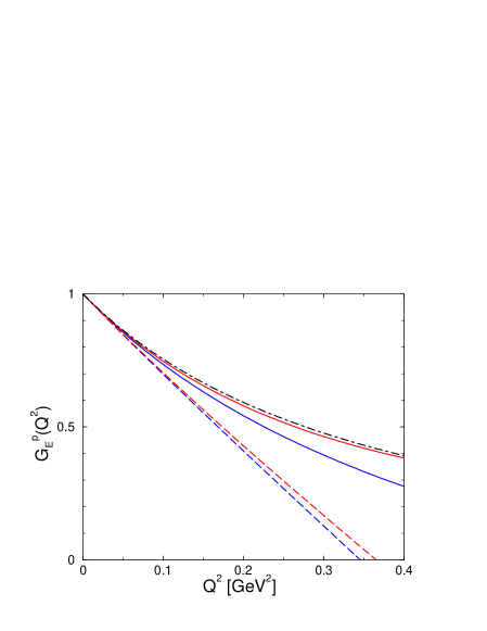
Figure 8: The proton electric form factor in relativistic baryon chiral perturbation theory including vector mesons (solid lines) to third (blue curve) and fourth (red curve) order. For comparison, the results without vector mesons are also shown (blue/red dashed line: third/fourth order). All LECs are determined by a fit to the proton charge radius as given by the dispersion theoretical result (black dot–dashed curve).

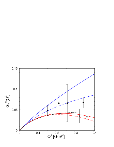
Figure 9: The neutron electric form factor in relativistic baryon chiral perturbation theory including vector mesons (solid lines) to third (blue curve) and fourth (red curve) order. For comparison, the results without vector mesons are also shown (blue/red dashed line: third/fourth order). All LECs are determined by a fit to the neutron charge radius. Also given is the result of the dispersion theoretical analysis (black dot–dashed curve). The data are from [22].

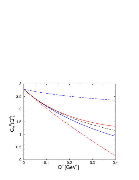
Figure 10: The proton magnetic form factor in relativistic baryon chiral perturbation theory including vector mesons (solid lines) to third (blue curve) and fourth (red curve) order. For comparison, the results without vector mesons are also shown (blue/red dashed line: third/fourth order). All LECs at third (fourth) order are determined by a fit to the proton magnetic moment (radius). Also given is the dispersion theoretical result (black dot–dashed curve).

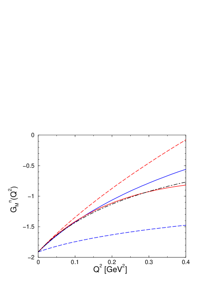
Figure 11: The neutron magnetic form factor in relativistic baryon chiral perturbation theory including vector mesons (solid lines) to third (blue curve) and fourth (red curve) order. For comparison, the results without vector mesons are also shown (blue/red dashed line: third/fourth order). All LECs at third (fourth) order are determined by a fit to the neutron magnetic moment (radius). Also given is the dispersion theoretical result (black dot–dashed curve).

The resulting electric and magnetic form factors of the proton and the neutron are shown in figs. 8–11. Consider the electric form factors first. The vector meson contribution already supplies sufficient curvature for an adequate description of the proton charge form factor at third order, cf. fig. 8. This is achieved without new adjustable parameters, but simply due to the higher order terms induced by the inclusion of the vector mesons. It is worth noting that at fourth order, the chiral plus vector meson representation is in almost perfect agreement with the result of the dispersive analysis up to momenta of $Q^{2}=0.4\,$GeV², i.e. for much higher momenta than considered so far in chiral perturbation theory approaches. However the already well–described neutron electric form factor, see fig. 9, is, at fourth order, only very mildly affected by the vector meson contribution, but is of course also most sensitive to the precise choice of the vector meson couplings. We only want to state that for a reasonable choice of these parameters, the good result of the chiral one–loop representation is not spoiled.

Turning now to the magnetic form factors, see figs. 10, 11, we find that both the third and the fourth order curves yield reasonable descriptions of the data, in both cases the fourth order results being slightly better than the respective third order ones. The latter show the right slope at the origin (which is fitted in the fourth order case), and all curves have approximately the right curvature, which is a bit stronger at fourth order.

We have, in addition, plotted the third and fourth order curves for $G_{E}^{p}$, $G_{M}^{p}$, and $G_{M}^{n}$ (including vector mesons), normalized and divided by the dipole form factor

$$G_{D}(Q^{2})=\frac{1}{\Bigl{(}1+Q^{2}/0.71\,{\rm GeV}^{2}\Bigr{)}^{2}}~{}~{},$$ (4.26)

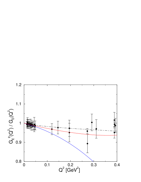
Figure 12: The proton electric form factor in relativistic baryon chiral perturbation theory including vector mesons to third (blue curve) and fourth (red curve) order, divided by the dipole form factor. For comparison, we show the dispersion theoretical result (black dot–dashed curve) and the world data available in this energy range.

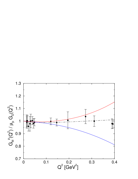
Figure 13: The proton magnetic form factor in relativistic baryon chiral perturbation theory including vector mesons to third (blue curve) and fourth (red curve) order, divided by the dipole form factor. For comparison, we show the dispersion theoretical result (black dot–dashed curve) and the world data available in this energy range.

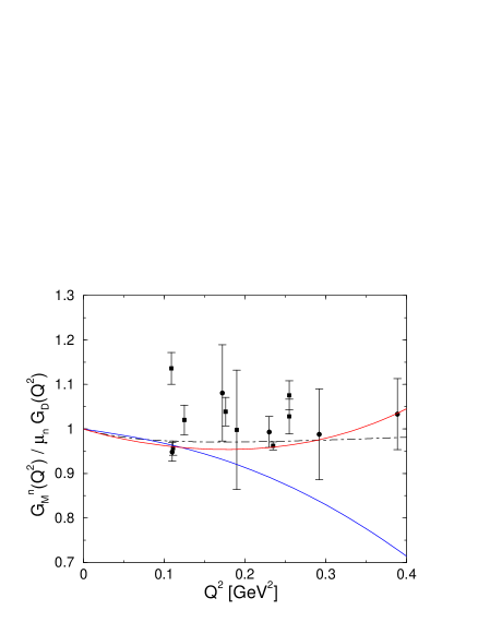
Figure 14: The neutron magnetic form factor in relativistic baryon chiral perturbation theory including vector mesons to third (blue curve) and fourth (red curve) order, divided by the dipole form factor. For comparison, we show the dispersion theoretical result (black dot–dashed curve) and the world data available in this energy range, where the data points denoted by squares (instead of circles) refer to the more recent measurements [36]. The older data can be traced back from [8].

see figs. 12–14. Here, again, we see that the fourth order prediction for the proton charge form factor agrees extremely well with the data up to $Q^{2}=0.4\,$GeV². For the neutron magnetic form factor, the fourth order curve, though rising above dipole and dispersion theoretical fit, still is within the error range given by the data, while the fourth order result for the proton magnetic form factor deviates from the data above $Q^{2}=0.3\,$GeV².

It is worth pointing out the following essential conclusions drawn from this discussion:

1. In section 3.4 we saw that the “prediction” of the magnetic radii in a third order calculation worsens considerably when comparing the relativistic and the heavy baryon approach. This observation indicated that the large contribution of the pion cloud to the magnetic radii was an artifact of the $1/m$–expansion to ${\cal O}(q^{3})$. Inspection of the third order curves including explicit vector meson effects shows that this reduction of the pion cloud effect is indeed consistent with the fairly conventional vector meson parameters, yielding in total excellent results for the magnetic radii which are still “predicted” and not fitted. We here show these “predictions” with the separate contributions of pion–cloud and vector mesons,

   $$(r_{M}^{p})^{2}\! = \!(r_{M}^{p})^{2}_{\pi}+(r_{M}^{p})^{2}_{\rm VM}=(0.18+0.49)\,{\rm fm}^{2}=(0.82\,{\rm fm})^{2}~{},$$ (4.27)

   $$(r_{M}^{n})^{2}\! = \!(r_{M}^{n})^{2}_{\pi}+(r_{M}^{n})^{2}_{\rm VM}=(0.26+0.44)\,{\rm fm}^{2}=(0.84\,{\rm fm})^{2}~{},$$ (4.28)

   in good agreement with the values from dispersion analyses, $r_{M}^{p}=0.836\,$fm and $r_{M}^{n}=0.889\,$fm. Note however that, although we did not fit any new parameters to the magnetic radii, additional experimental information enters via the vector meson couplings which in turn have been fitted to the form factors in the dispersive approach.

2. This analysis indicates that a “strict” ChPT calculation to higher–than–fourth order is probably only moderately sensible. Apart from various two–loop contributions which amount only to vertex corrections of diagrams already present in the one–loop case, the major “new” contribution is the three–pion continuum entering the isoscalar form factors, which was already shown to yield a negligibly small correction to the $\omega/\phi$–peak in the isoscalar spectral function [5]. Therefore, an analysis to ${\cal O}(q^{5})$ or ${\cal O}(q^{6})$ would basically result in fitting new counterterm parameters in order to reproduce the resonance contributions considered explicitly here. Apart from that, it is so far not known how to generalize the infrared regularization scheme to higher loop orders, and therefore for such a higher order calculation one would have to retrieve to the non–relativistic formalism.

4.3 Remarks on resonance saturation

As we have not assumed resonance saturation of the various low energy constants, but taken the resonance parameters from elsewhere and refitted the contact terms, we may now check how well resonance saturation by the lowest lying vector mesons actually works. Table 1 shows the values for the low energy constants, fitted at third and fourth order, with and without vector meson contributions.

	$q^{3}$	$q^{4}$	$q^{3}+$VM	$q^{4}+$VM
$c_{6}$	5.03	4.77	0.20	$-$0.06
$c_{7}$	$-$2.72	$-$2.55	$-$0.27	$-$0.09
$d_{6}^{r}$	0.67	0.74	1.34	1.40
$d_{7}$	$-$0.70	$-$0.69	$-$0.04	$-$0.03
$e_{54}$	—	0.26	—	$-$0.04
$e_{74}^{r}$	—	1.65	—	$-$1.15

Table 1: Values for the various low energy constants, with and without vector meson contributions. Note that the third and the fourth columns, strictly speaking, refer to the LECs $\hat{\alpha}_{i}$ instead of $\alpha_{i}$. $c_{6},\,c_{7}$ are dimensionless, the $d_{i}$ are given in GeV^-2, the $e_{i}$ in GeV^-3.

The vector meson contribution to the LEC $c_{4}$ as given in eq. (4.24) numerically amounts to $1.6\,$GeV^-1 (see also [26]) which reduces the value of $\hat{c}_{4}$ by about 50%. This remainder which is due to (mainly) $\Delta$ and a small Roper contribution is still represented by a contact term.

We conclude that the low energy constants entering the magnetic moments ($c_{6},\,c_{7}$) as well as those fitted to the isoscalar radii, both electric ($d_{7}$) and magnetic ($e_{54}$), are nearly perfectly saturated by the lowest lying vector meson nonet, while the contact terms entering the isovector radii ($d_{6},\,e_{74}$) are not at all. This can be interpreted to the effect that $\omega$ and $\phi$ are already sufficient to describe the isoscalar channel of the vector form factors to good accuracy, while higher resonances are mandatory for an adequate description of the isovector form factors. This is in agreement with what is found in dispersive analyses. However this does not necessarily invalidate our approach, as these higher resonances have much larger masses (the $\rho(1450)$ being the lowest lying of them) and therefore will hardly contribute to the curvature of the form factors (which is the change we are looking for, compared to linear contact terms).

5 Summary

We have studied the electromagnetic form factors of the nucleon in a manifestly Lorentz invariant form of baryon chiral perturbation theory to one–loop (fourth) order. As discussed, in this scheme based on the so–called infrared regularization of loop graphs, one is able to set up a systematic power counting scheme in harmony with the strictures from analyticity. The pertinent results of our investigation can be summarized as follows:

• To fourth order, the neutron and proton electric form factors each contain one low–energy constant which can be fixed from the empirical information on the corresponding radii. This gives a good description of the neutron charge form factor up to four–momentum transfer squared of $Q^{2}=0.4\,$GeV² and, furthermore, exhibits convergence in that the corrections when going from third to fourth order are small. This is in contrast to the heavy baryon expansion and can be traced back to the proper resummation of the recoil terms in the relativistic expansion. For the electric form factor of the proton, the one–loop representation gives too little curvature and thus deviates from the data already at $Q^{2}\simeq 0.2\,$GeV², similar to the heavy baryon description. However, no large fourth order corrections are found below $Q^{2}=0.4\,$GeV².

• To third order, the momentum dependence of the magnetic proton and neutron form factor is given parameter–free. The $1/m$ corrections present in our approach worsen the prediction for the magnetic radii based on the leading chiral singularities, like e.g. in the heavy baryon approach. The leading chiral limit behavior is not a good approximation for the Goldstone boson contribution to the magnetic radii. At fourth order, the magnetic radii can be fixed. Again, there is not enough curvature in the one–loop representation and one observes large corrections when going from third to fourth order already at $Q^{2}\simeq 0.1\,$GeV².

• We have demonstrated explicitly that the spectral functions of the isovector form factors have the correct threshold behavior. The strong momentum–dependence of these spectral functions close to threshold is due to the branch point singularity on the second Riemann sheet inherited from the $\pi\pi\to\bar{N}{N}$ P–wave partial wave amplitudes.

• We have included the low–lying vector mesons $\rho$, $\omega$, $\phi$ in a chirally symmetric manner based on an antisymmetric tensor field representation. This does not introduce any new parameters since these (masses and coupling constants) are taken from the PDG tables and from a dispersion theoretical analysis. Refitting the previously defined low–energy constants by subtracting the vector meson contribution, we find a good description of all four form factors already at third order, with small fourth order contributions, which further improve the theoretical description. In particular, we demonstrate that the vector meson contributions cancel to a large extent in the neutron charge form factor, thus solidifying the result obtained in the chiral expansion.

• The inclusion of vector mesons allows to investigate the resonance saturation hypothesis for these couplings. We find that the couplings related to the magnetic moments and the isoscalar radii are almost completely saturated by the low–lying vector mesons. This is, however, not the case for the LECs entering the isovector radii. This can be traced back to the fact that while the $\omega$ and the $\phi$ already give a good description of the isoscalar form factors, for the isovector ones one has to include higher mass states than the $\rho$, in agreement with findings from dispersion theory.

Appendix A Loop integrals

In this appendix, we define the loop integrals needed in this paper and evaluate them in the infrared regularization scheme. Several of these results have already been given in [6].

A.1 Definition of the loop integrals

We use the following notation:

$$p^{\prime}_{\mu}+p_{\mu}=Q_{\mu}~{},\qquad p^{\prime}_{\mu}-p_{\mu}=q_{\mu}~{},\qquad t=q^{2}~{},$$

$$\mu=\frac{M_{\pi}}{m_{N}}~{},\qquad\tau=\frac{t}{m_{N}^{2}}~{},\qquad\theta=\frac{t}{M_{\pi}^{2}}~{}.$$

In addition, everywhere except in the loop integrals with just one meson and one nucleon propagator, we only need the case where the nucleon momenta are on–shell, i.e. $p^{2}=p^{\prime 2}=m_{N}^{2}$.

Define the following loop integrals:

$$\frac{1}{i}\int_{I}\frac{d^{d}k}{(2\pi)^{d}}\frac{1}{M_{\pi}^{2}-k^{2}} = \Delta_{\pi}~{}~{},$$ (A.1)

$$\frac{1}{i}\int_{I}\frac{d^{d}k}{(2\pi)^{d}}\frac{1}{[M_{\pi}^{2}-k^{2}][M_{\pi}^{2}-(k+q)^{2}]} = J(t)~{}~{},$$ (A.2)

$$\frac{1}{i}\int_{I}\frac{d^{d}k}{(2\pi)^{d}}\frac{k_{\mu}}{[M_{\pi}^{2}-k^{2}][M_{\pi}^{2}-(k+q)^{2}]} = -\frac{1}{2}q_{\mu}J(t)~{}~{},$$ (A.3)

$$\frac{1}{i}\int_{I}\frac{d^{d}k}{(2\pi)^{d}}\frac{k_{\mu}k_{\nu}}{[M_{\pi}^{2}-k^{2}][M_{\pi}^{2}-(k+q)^{2}]} = \Bigl{(}q_{\mu}q_{\nu}-g_{\mu\nu}t\Bigr{)}\,J^{(1)}(t)$$ (A.4)

$$+ q_{\mu}q_{\nu}\,J^{(2)}(t)~{}~{},$$

$$\frac{1}{i}\int_{I}\frac{d^{d}k}{(2\pi)^{d}}\frac{1}{[M_{\pi}^{2}-k^{2}][m_{N}^{2}-(p-k)^{2}]} = I(p^{2})~{}~{},$$ (A.5)

$$\frac{1}{i}\int_{I}\frac{d^{d}k}{(2\pi)^{d}}\frac{k_{\mu}}{[M_{\pi}^{2}-k^{2}][m_{N}^{2}-(p-k)^{2}]} = p_{\mu}\,I^{(1)}(p^{2})~{}~{},$$ (A.6)

$$\frac{1}{i}\int_{I}\frac{d^{d}k}{(2\pi)^{d}}\frac{1}{[M_{\pi}^{2}-k^{2}][m_{N}^{2}-(p-k)^{2}][m_{N}^{2}-(p^{\prime}-k)^{2}]} = I_{A}(t)~{}~{},$$ (A.7)

$$\frac{1}{i}\int_{I}\frac{d^{d}k}{(2\pi)^{d}}\frac{k_{\mu}}{[M_{\pi}^{2}-k^{2}][m_{N}^{2}-(p-k)^{2}][m_{N}^{2}-(p^{\prime}-k)^{2}]} = Q_{\mu}\,I_{A}^{(1)}(t)~{}~{},$$ (A.8)

$$\frac{1}{i}\int_{I}\frac{d^{d}k}{(2\pi)^{d}}\frac{k_{\mu}k_{\nu}}{[M_{\pi}^{2}-k^{2}][m_{N}^{2}-(p-k)^{2}][m_{N}^{2}-(p^{\prime}-k)^{2}]} = g_{\mu\nu}\,I_{A}^{(2)}(t)$$ (A.9)

$$+ Q_{\mu}Q_{\nu}\,I_{A}^{(3)}(t)$$

$$+ q_{\mu}q_{\nu}\,I_{A}^{(4)}(t)~{}~{},$$

$$\frac{1}{i}\int_{I}\frac{d^{d}k}{(2\pi)^{d}}\frac{1}{[M_{\pi}^{2}-k^{2}][M_{\pi}^{2}-(k+q)^{2}][m_{N}^{2}-(p-k)^{2}]} = I_{21}(t)~{}~{},$$ (A.10)

$$\frac{1}{i}\int_{I}\frac{d^{d}k}{(2\pi)^{d}}\frac{k_{\mu}}{[M_{\pi}^{2}-k^{2}][M_{\pi}^{2}-(k+q)^{2}][m_{N}^{2}-(p-k)^{2}]} = Q_{\mu}\,I_{21}^{Q}(t)$$ (A.11)

$$- \frac{1}{2}q_{\mu}\,I_{21}(t)~{}~{},$$

$$\frac{1}{i}\int_{I}\frac{d^{d}k}{(2\pi)^{d}}\frac{k_{\mu}k_{\nu}}{[M_{\pi}^{2}-k^{2}][M_{\pi}^{2}-(k+q)^{2}][m_{N}^{2}-(p-k)^{2}]} = g_{\mu\nu}\,I_{21}^{00}(t)$$

$$+ Q_{\mu}Q_{\nu}\,I_{21}^{QQ}(t)$$

$$+ q_{\mu}q_{\nu}\,I_{21}^{qq}(t)$$

$$- \Bigl{(}q_{\mu}Q_{\nu}+q_{\nu}Q_{\mu}\Bigr{)}\,\frac{1}{2}I_{21}^{Q}(t)~{}~{},$$

where $\int_{I}$ symbolizes loop integration according to the infrared regularization scheme.

A.2 Reduction of the tensorial loop integrals

The reduction of the tensorial loop integrals to the corresponding scalar ones can be performed in the standard way and leads to the following results:

$$J^{(1)}(t) = \frac{1}{4(d-1)\,t}\Bigl{\{}(t-4M_{\pi}^{2})J(t)+2\Delta_{\pi}\Bigr{\}}~{}~{},$$ (A.13)

$$J^{(2)}(t) = \frac{1}{4}J(t)-\frac{1}{2t}\Delta_{\pi}~{}~{},$$ (A.14)

$$I^{(1)}(p^{2}) = \frac{1}{2p^{2}}\Bigl{\{}(p^{2}-m_{N}^{2}+M_{\pi}^{2})I(p^{2})+\Delta_{\pi}\Bigr{\}}~{}~{},$$ (A.15)

$$I_{A}^{(1)}(t) = \frac{1}{4m_{N}^{2}-t}\Bigl{\{}I(m_{N}^{2})+M_{\pi}^{2}I_{A}(t)\Bigr{\}}~{}~{},$$ (A.16)

$$I_{A}^{(2)}(t) = \frac{1}{d-2}\Bigl{\{}I_{A}(t)-I_{A}^{(1)}(t)\Bigr{\}}M_{\pi}^{2}~{}~{},$$ (A.17)

$$I_{A}^{(3)}(t) = \frac{1}{(d-2)(4m_{N}^{2}-t)}\biggl{\{}\Bigl{(}(d-1)I_{A}^{(1)}(t)-I_{A}(t)\Bigr{)}M_{\pi}^{2}+\frac{d-2}{2}I^{(1)}(m_{N}^{2})\biggr{\}}~{},~{}$$ (A.18)

$$I_{A}^{(4)}(t) = \frac{1}{(d-2)\,t}\biggl{\{}\Bigl{(}I_{A}^{(1)}(t)-I_{A}(t)\Bigr{)}M_{\pi}^{2}-\frac{d-2}{2}I^{(1)}(m_{N}^{2})\biggr{\}}~{}~{},$$ (A.19)

$$I_{21}^{Q}(t) = \frac{1}{2(4m_{N}^{2}-t)}\Bigl{\{}(2M_{\pi}^{2}-t)I_{21}(t)-2I(m_{N}^{2})+2J(t)\Bigr{\}}~{}~{},$$ (A.20)

$$I_{21}^{00}(t) = \frac{1}{4(2-d)}\Bigl{\{}2I(m_{N}^{2})-(4M_{\pi}^{2}-t)I_{21}(t)+2(2M_{\pi}^{2}-t)I_{21}^{Q}(t)\Bigr{\}}~{}~{},$$ (A.21)

$$I_{21}^{QQ}(t) = \frac{1}{4(d-2)(4m_{N}^{2}-t)}\biggl{\{}2I(m_{N}^{2})-2(d-2)I^{(1)}(m_{N}^{2})$$ (A.22)

$$\qquad\qquad-(4M_{\pi}^{2}-t)I_{21}(t)+2(d-1)(2M_{\pi}^{2}-t)I_{21}^{Q}(t)\biggr{\}}~{}~{},$$

$$I_{21}^{qq}(t) = \frac{1}{4(d-2)t}\biggl{\{}-2(d-3)I(m_{N}^{2})+2(d-2)I^{(1)}(m_{N}^{2})$$ (A.23)

$$\qquad\qquad-\Bigl{(}4M_{\pi}^{2}-(d-1)\,t\Bigr{)}I_{21}(t)+2(2M_{\pi}^{2}-t)I_{21}^{Q}(t)\biggr{\}}~{}~{}.$$

A.3 Scalar loop integrals

The scalar loop integrals are found to be

$$\Delta_{\pi} = 2M_{\pi}^{2}\biggl{\{}L+\frac{1}{16\pi^{2}}\log\mu\biggr{\}}~{}~{},$$ (A.24)

$$J(t) = -2\biggl{\{}L+\frac{1}{16\pi^{2}}\log\mu\biggr{\}}-\frac{1}{16\pi^{2}}\Bigl{(}1+k(t)\Bigr{)}~{}~{},$$ (A.25)

$$I(m_{N}^{2}) = -\mu^{2}\biggl{(}L+\frac{1}{16\pi^{2}}\log\mu\biggr{)}+\frac{\mu}{16\pi^{2}}\biggl{\{}\frac{\mu}{2}-\sqrt{4-\mu^{2}}\arccos\biggl{(}-\frac{\mu}{2}\biggr{)}\biggr{\}}~{}~{},$$ (A.26)

$$I_{A}(t) = -\frac{f(t)}{m_{N}^{2}}\biggl{\{}L+\frac{1}{16\pi^{2}}\biggl{(}\log\mu+\frac{1}{2}\biggr{)}\biggr{\}}+\frac{1}{16\pi^{2}}\frac{\mu}{2m_{N}^{2}}g(t)~{}~{},$$ (A.27)

$$I_{21}(t) = \frac{f(t)}{m_{N}^{2}}\biggl{\{}L+\frac{1}{16\pi^{2}}\biggl{(}\log\mu+\frac{1}{2}\biggr{)}\biggr{\}}+\frac{1}{16\pi^{2}}\frac{1}{2m_{N}^{2}}\biggl{(}h_{1}(t)+\frac{2-\mu^{2}}{\mu}h_{2}(t)\biggr{)}~{},~{}$$ (A.28)

where the following loop functions have been reduced to integrals over one Feynman parameter:

$$k(t) = \int_{0}^{1}dx\log\Bigl{(}1-x(1-x)\,\theta\Bigr{)}=\sqrt{\frac{4-\theta}{-\theta}}\log\biggl{(}\frac{\sqrt{4-\theta}+\sqrt{-\theta}}{\sqrt{4-\theta}-\sqrt{-\theta}}\biggr{)}-2~{}~{},$$ (A.29)

$$f(t) = \int_{0}^{1}dx\frac{dx}{1-x(1-x)\,\tau}\,=\,\frac{2}{\sqrt{-\tau\smash{(4-\tau)}}}\log\biggl{(}\frac{\sqrt{4-\tau}+\sqrt{-\tau}}{\sqrt{4-\tau}-\sqrt{-\tau}}\biggr{)}~{}~{},$$ (A.30)

$$g(t) = \int_{0}^{1}dx\frac{\arccos\Bigl{(}-\frac{\mu}{2\sqrt{1-x(1-x)\tau}}\Bigr{)}}{\Bigl{(}1-x(1-x)\,\tau\Bigr{)}\sqrt{1-\frac{\mu^{2}}{4}-x(1-x)\,\tau}}~{}~{},$$ (A.31)

$$h_{1}(t) = \int_{0}^{1}dx\frac{\log\Bigl{(}1-x(1-x)\,\theta\Bigr{)}}{1-x(1-x)\,\tau}~{}~{},$$ (A.32)

$$h_{2}(t) = \int_{0}^{1}dx\frac{\arccos\Bigl{(}-\frac{\mu\bigl{(}\frac{1}{2}-x(1-x)\,\theta\bigr{)}}{\sqrt{(1-x(1-x)\,\tau)\,(1-x(1-x)\,\theta)}}\Bigr{)}}{\Bigl{(}1-x(1-x)\,\tau\Bigr{)}\sqrt{1-\frac{\mu^{2}}{4}-x(1-x)\,\theta}}~{}~{}.$$ (A.33)

Appendix B Form factor contributions from separate diagrams

In this section, we give the contributions to the form factors $F_{1}(t),\,F_{2}(t)$, coming from the various diagrams shown in fig. 2 .

B.1 Contributions to $F_{1}$

$$E_{1+3} = 1-\Bigl{(}\tau^{3}\,d_{6}+2\,d_{7}\Bigr{)}\,t~{}~{},$$ (B.1)

$$E_{5} = \frac{g_{A}^{2}}{8F_{\pi}^{2}}\,(3-\tau^{3})\,\Bigl{\{}\Delta_{\pi}-4m_{N}^{2}I^{(1)}(m_{N}^{2})-4m_{N}^{2}M_{\pi}^{2}I_{A}(t)$$ (B.2)

$$\qquad\qquad\qquad+8m_{N}^{2}I_{A}^{(2)}(t)+32m_{N}^{4}I_{A}^{(3)}(t)\Bigr{\}}~{}~{},$$

$$E_{6} = -\frac{g_{A}^{2}}{F_{\pi}^{2}}\,\tau^{3}\,\Bigl{\{}tJ^{(1)}(t)+4m_{N}^{2}I_{21}^{00}(t)+16m_{N}^{4}I_{21}^{QQ}(t)\Bigr{\}}~{}~{},$$ (B.3)

$$E_{7} = \frac{g_{A}^{2}}{F_{\pi}^{2}}\,\tau^{3}\,\Bigl{\{}\Delta_{\pi}-2m_{N}^{2}I^{(1)}(m_{N}^{2})\Bigr{\}}~{}~{},$$ (B.4)

$$E_{8} = -\frac{\tau^{3}}{2F_{\pi}^{2}}\,\Delta_{\pi}~{}~{},$$ (B.5)

$$E_{9} = \frac{\tau^{3}}{F_{\pi}^{2}}\,t\,J^{(1)}(t)~{}~{},$$ (B.6)

$$E_{10} = \frac{m_{N}^{2}g_{A}^{2}}{F_{\pi}^{2}}\Bigl{(}(3-\tau^{3})c_{6}+6c_{7}\Bigr{)}\,t\,I_{A}^{(3)}(t)~{}~{},$$ (B.7)

$$E_{11} = \frac{3M_{\pi}^{2}}{4m_{N}F_{\pi}^{2}}\,(1+\tau^{3})\,c_{2}\,\biggl{\{}\Delta_{\pi}-\frac{M_{\pi}^{2}}{32\pi^{2}}\biggr{\}}~{}~{}.$$ (B.8)

B.2 Contributions to $F_{2}$

$$M_{2+3+4} = \frac{1}{2}(1+\tau^{3})\,c_{6}+c_{7}+\Bigl{(}\tau^{3}\,d_{6}+2\,d_{7}\Bigr{)}\,t+2m_{N}\Bigl{(}2\,e_{54}+\tau^{3}\,e_{74}\Bigr{)}\,t$$ (B.9)

$$-8m_{N}M_{\pi}^{2}\Bigl{(}2\,e_{105}+\tau^{3}\,e_{106}\Bigr{)}~{}~{},$$

$$M_{5} = -\frac{g_{A}^{2}}{F_{\pi}^{2}}\,(3-\tau^{3})\,4m_{N}^{4}\,I_{A}^{(3)}(t)~{}~{},$$ (B.10)

$$M_{6} = \frac{g_{A}^{2}}{F_{\pi}^{2}}\,\tau^{3}\,16m_{N}^{4}I_{21}^{QQ}(t)~{}~{},$$ (B.11)

$$M_{10} = -\frac{m_{N}^{4}g_{A}^{2}}{8F_{\pi}^{2}}\Bigl{(}(3-\tau^{3})\,c_{6}+6c_{7}\Bigr{)}\Bigl{\{}\Delta_{\pi}-4m_{N}^{2}I^{(1)}(m_{N}^{2})+4m_{N}^{2}M_{\pi}^{2}I_{A}(t)$$ (B.12)

$$\qquad-16m_{N}^{2}I_{A}^{(2)}(t)+8m_{N}^{2}t\Bigl{(}I_{A}^{(3)}(t)-I_{A}^{(4)}(t)\Bigr{)}\Bigr{\}}~{}~{},$$

$$M_{11} = -\frac{3M_{\pi}^{2}}{4m_{N}F_{\pi}^{2}}\,(1+\tau^{3})\,c_{2}\,\biggl{\{}\Delta_{\pi}-\frac{M_{\pi}^{2}}{32\pi^{2}}\biggr{\}}-\frac{\tau^{3}}{2F_{\pi}^{2}}\,c_{6}\,\Delta_{\pi}~{}~{},$$ (B.13)

$$M_{12} = \frac{4m_{N}}{F_{\pi}^{2}}\,\tau^{3}\,c_{4}\,t\,J^{(1)}(t)~{}~{}.$$ (B.14)

B.3 Z–factor

We here spell out the Z–factor needed for wave function renormalization up to fourth order. For the evaluation of the form factor $F_{1}$, the nucleon charge has to be multiplied by $Z_{N}$, while for $F_{2}$, the anomalous magnetic moment (a second order contribution) only has to be renormalized by the Z–factor up to third order, i.e. the term $\sim c_{2}$ can be dropped.

$$Z_{N} = 1\,+\,\frac{3g_{A}^{2}}{4F_{\pi}^{2}}\biggl{\{}M_{\pi}^{2}I(m_{N}^{2})-2m_{N}^{2}I^{(1)}(m_{N}^{2})+4m_{N}^{2}M_{\pi}^{2}\Bigl{(}I_{A}(0)-2I_{A}^{(1)}(0)\Bigr{)}\biggr{\}}$$ (B.15)

$$\quad-\,c_{2}\,\frac{3M_{\pi}^{2}}{2m_{N}F_{\pi}^{2}}\biggl{(}\Delta_{\pi}-\frac{M_{\pi}^{2}}{32\pi^{2}}\biggr{)}~{}~{}.$$

Appendix C Imaginary parts and spectral functions

Out of the diagrams depicted in fig. 2, only graphs (6), (9), and (12) contribute to the spectral functions of the isovector form factors in the low energy region, i.e. starting at the threshold $t=4M_{\pi}^{2}$. The separate contributions can be calculated either from the imaginary parts of the two basic loop functions involved (see also [2]),

$${\rm Im}\,J(t) = \frac{1}{16\pi}\,\sqrt{1-\frac{4M_{\pi}^{2}}{t}}~{}~{},$$ (C.1)

$${\rm Im}\,I_{21}(t) = \frac{1}{8\pi}\,\frac{1}{\sqrt{t(4m_{N}^{2}-t)}}\,\arctan\frac{\sqrt{(4m_{N}^{2}-t)(t-4M_{\pi}^{2})}}{t-2M_{\pi}^{2}}~{}~{},$$ (C.2)

or directly by using Cutkosky rules. This leads to the following expressions:

$${\rm Im}\,E_{6} = \frac{\tau^{3}\,g_{A}^{2}}{192\pi F_{\pi}^{2}\,(4m_{N}^{2}-t)^{2}}\,\sqrt{1-\frac{4M_{\pi}^{2}}{t}}$$

$$\times \Biggl{\{}16m_{N}^{4}\Bigl{(}5t-8M_{\pi}^{2}\Bigr{)}+4m_{N}^{2}\,t\,\Bigl{(}5t-14M_{\pi}^{2}\Bigr{)}-t^{2}\Bigl{(}t-4M_{\pi}^{2}\Bigr{)}$$

$$\quad-48m_{N}^{2}\,\frac{m_{N}^{2}\Bigl{(}3t^{2}-12M_{\pi}^{2}t+8M_{\pi}^{4}\Bigr{)}+M_{\pi}^{4}t}{\sqrt{(4m_{N}^{2}-t)(t-4M_{\pi}^{2})}}\arctan\frac{\sqrt{(4m_{N}^{2}-t)(t-4M_{\pi}^{2})}}{t-2M_{\pi}^{2}}\Biggr{\}}~{}~{},$$

$${\rm Im}\,M_{6} = \frac{\tau^{3}\,g_{A}^{2}\,m_{N}^{4}}{4\pi F_{\pi}^{2}\,(4m_{N}^{2}-t)^{2}}\,\sqrt{1-\frac{4M_{\pi}^{2}}{t}}\,\Biggl{\{}-3\Bigl{(}t-2M_{\pi}^{2}\Bigr{)}$$ (C.4)

$$\quad+2\,\frac{\Bigl{(}2m_{N}^{2}+t\Bigr{)}\Bigl{(}t-4M_{\pi}^{2}\Bigr{)}+6M_{\pi}^{4}}{\sqrt{(4m_{N}^{2}-t)(t-4M_{\pi}^{2})}}\arctan\frac{\sqrt{(4m_{N}^{2}-t)(t-4M_{\pi}^{2})}}{t-2M_{\pi}^{2}}\Biggr{\}}~{}~{},$$

$${\rm Im}\,E_{9} = \frac{\tau^{3}}{192\pi F_{\pi}^{2}}\,\frac{(t-4M_{\pi}^{2})^{3/2}}{t^{1/2}}~{}~{},$$ (C.5)

$${\rm Im}\,M_{12} = \frac{m_{N}\,c_{4}\,\tau^{3}}{48\pi F_{\pi}^{2}}\,\frac{(t-4M_{\pi}^{2})^{3/2}}{t^{1/2}}~{}~{}.$$ (C.6)

For these results, see also [2, 5].

 

Figures

Figure 1: Lowest order loop diagrams contributing to the mass renormalization of (a) the pion at ${\cal O}(q^{4})$, and (b) the nucleon at ${\cal O}(q^{3})$. Solid and dashed lines refer to nucleons and pions, respectively.

 

Figure 2: Feynman diagrams contributing to the electromagnetic form factors up to fourth order. Solid, dashed, and wiggly lines refer to nucleons, pions, and the vector source, respectively. Vertices denoted by a heavy dot / a square / a diamond refer to insertions from the second / third / fourth order chiral Lagrangian, respectively. Diagrams contributing via wave function renormalization only are not shown.

 

 

 

 

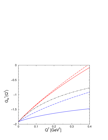
Figure 6: The neutron magnetic form factor in relativistic baryon chiral perturbation theory (solid lines) to third (blue curve) and fourth (red curve) order. For comparison, the results of the heavy baryon approach are also shown (blue/red dashed line: third/fourth order). The third (fourth) order LECs are determined by a fit to the neutron magnetic moment (radius). Also given is the dispersion theoretical result (black dot–dashed curve).

 

Figure 7: Feynman diagrams including explicit vector meson contributions to the electromagnetic form factors up to fourth order. Solid, dashed, double–dashed, and wiggly lines refer to nucleons, pions, vector mesons, and the vector source, respectively. The vertex denoted by an open dot refers to the vector coupling of the vector mesons to the nucleon which is of subleading chiral order as compared to the tensor coupling.

References

• [1] M.A.B. Bég and A. Zepeda, Phys. Rev. D6 (1972) 2912.
• [2] J. Gasser, M.E. Sainio, and A. Švarc, Nucl. Phys. B307 (1988) 779.
• [3] V. Bernard, N. Kaiser, J. Kambor, and U.-G. Meißner, Nucl. Phys. B388 (1992) 315.
• [4] V. Bernard, H.W. Fearing, T.R. Hemmert, and U.-G. Meißner, Nucl. Phys. A635 (1998) 121; (E) Nucl. Phys. A642 (1998) 563.
• [5] V. Bernard, N. Kaiser, and U.-G. Meißner, Nucl. Phys. A611 (1996) 429.
• [6] T. Becher and H. Leutwyler, Eur. Phys. J. C9 (1999) 643.
• [7] G. Höhler et al., Nucl. Phys. B114 (1976) 389.
• [8] P. Mergell, U.-G. Meißner, and D. Drechsel, Nucl. Phys. A596 (1996) 367.
• [9] H.-W. Hammer, U.-G. Meißner, and D. Drechsel, Phys. Lett. B385 (1996) 343.
• [10] U.-G. Meißner, Nucl. Phys. A666&667 (2000) 51c.
• [11] G.G. Petratos, Nucl. Phys. A666&667 (2000) 61c.
• [12] H. Leutwyler, Ann. Phys. (NY) 235 (1994) 165.
• [13] V. Bernard, N. Kaiser, and U.-G. Meißner, Int. J. Mod. Phys. E4 (1995) 193.
• [14] N. Fettes, U.-G. Meißner, and S. Steininger, Nucl. Phys. A640 (1998) 199.
• [15] N. Fettes, U.-G. Meißner, M. Mojžiš, and S. Steininger, Ann. Phys. (NY), in print.
• [16] U.-G. Meißner, in Themes in strong interaction physics, J. Goity (ed.), World Scientific (1998), hep-ph/9711365.
• [17] H.-B. Tang, hep-ph/9607436; P.J. Ellis and H.-B. Tang, Phys. Rev. C57 (1998) 3356.
• [18] G. Ecker, Phys. Lett. B336 (1994) 508.
• [19] P. Büttiker and U.-G. Meißner, Nucl. Phys. A668 (2000) 97.
• [20] R. Rosenfelder, Phys. Lett. B479 (2000) 381.
• [21] K. Melnikov and T. van Ritbergen, Phys. Rev. Lett. 84 (2000) 1673.
• [22] T. Eden et al., Phys. Rev. C50 (1994) R1749; M. Meyerhoff et al., Phys. Lett. B327 (1994) 201; C. Herberg et al, Eur. Phys. J. A5 (1999) 131; I. Passchier et al., Phys. Rev. Lett. 82 (1999) 4988; M. Ostrick et al., Phys. Rev. Lett. 83 (1999) 276; J. Becker et al., Eur. Phys. J. A6 (1999) 329.
• [23] T.R. Hemmert and G. Gellas, unpublished.
• [24] B. Kubis, T.R. Hemmert, and U.-G. Meißner, Phys. Lett. B456 (1999) 240.
• [25] W.R. Frazer and J.R. Fulco, Phys. Rev. 117 (1960) 1603, 1609.
• [26] V. Bernard, N. Kaiser, and U.-G. Meißner, Nucl. Phys. A615 (1997) 483.
• [27] J. Gasser and H. Leutwyler, Ann. Phys. (NY) 158 (1984) 142.
• [28] U.-G. Meißner, Phys. Rept. 161 (1988) 213.
• [29] M. Bando, T. Kugo, and K. Yamawaki, Phys. Rept. 164 (1988) 217.
• [30] B. Borasoy and U.-G. Meißner, Int. J. Mod. Phys. A11 (1996) 5183.
• [31] G. Ecker, J. Gasser, A. Pich, and E. de Rafael, Nucl. Phys. B 321 (1989) 311; G. Ecker, J. Gasser, H. Leutwyler, A. Pich, and E. de Rafael, Phys. Lett. B223 (1989) 425.
• [32] U.-G. Meißner and J.A. Oller, Nucl. Phys. A673 (2000) 311.
• [33] J. Bijnens, P. Gosdzinsky, and P. Talavera, Nucl. Phys. B501 (1997) 495; JHEP 9801 (1998) 014; Phys. Lett. B429 (1998) 111.
• [34] E. Jenkins, A. Manohar, and M. Wise, Phys. Rev. Lett. 97 (1995) 2272.
• [35] K. Kawarabayashi and M. Suzuki, Phys. Rev. Lett. 16 (1966) 255; Fayyazuddin and Riazuddin, Phys. Rev. 147 (1966) 1071.
• [36] P. Markowitz et al., Phys. Rev. C48 (1993) R5; H. Gao et al., Phys. Rev. C50 (1994) R546; H. Anklin et al., Phys. Lett. B336 (1994) 313; E.E.W. Bruins et al., Phys. Rev. Lett. 75 (1995) 21; H. Anklin et al., Phys. Lett. B428 (1998) 248.