Abstract

We introduce the standard model of elementary particles and discuss the reasons why we have to modify it. Emphasis is put on the indications from the neutrinos and on the role of the Higgs particle; some promising theoretical ideas, like quark-lepton symmetry, existence of super-heavy “right-handed” neutrinos, grand unification and supersymmetry at the weak scale, are introduced and shortly discussed.

1 The standard model of elementary particles

In this section we define the standard model of elementary particles (SM) by introducing the particle content and the parameters of this model. We aim at giving a short introduction, at illustrating how this model is used, and at discussing (some of) its merits and limitations (to go deeper in the subjects touched, one could make reference to the seminal papers on the SM [1], to books and reviews [2, 3], and to the Particle Data Group biannual report [4]).

1.1 The basic blocks

There are two groups of spin 1/2 particles, quark and leptons, divided in 4 groups with different values of the electric charge $Q$

$$\mbox{\sc MATTER FERMIONS}\ \ \ \left\{\begin{array}[]{lllll}\mbox{\bf leptons}&Q=0,&\nu_{\rm e}\ \nu_{\mu}\ \nu_{\tau};&Q=-1,&\rm{e}\ \mu\ \tau.\\ \mbox{\bf quarks}&Q=2/3,&u\ c\ t;&Q=-1/3,&d\ s\ b.\end{array}\right.$$

(respectively named: e-, mu- and tau-neutrinos; electron, muon, tau; up, charm and top quarks; down, strange and bottom quarks; recall the existence of their anti-particles, with opposite charge). A different mass distinguishes among the three particles in each group (neutrino masses are to a certain extent special, and we will discuss them in a few pages). Thence, the fundamental particles can be arranged in three “families”, with increasingly heavier members–but otherwise identical. Free quarks have never been observed. It is thought that they can manifest as such only in very energetic processes; and that they necessarily bind to form the “hadrons”

$$\mbox{\sc HADRONS}\ \ \ \left\{\begin{array}[]{ll}\mbox{{\bf mesons} ($q\bar{q}$ states--bosons)}&\ \ \ \ \ \ \pi^{\pm}\ \pi^{0}\ K\ \rho\ ...\ \phi\ ...\ J/\Psi\ ...\\ \mbox{{\bf baryons} ($qqq$ states--fermions)}&\ \ \ \ \ \ p\ n\ \Delta^{\pm}\ ...\ \Lambda\ ...\ \Lambda_{b}\ ...\end{array}\right.$$

the binding is provided by “strong” interactions, a prerogative of the quarks; the forces between nuclei are regarded as residual strong interactions.

Actually, the list of stable spin 1/2 particles is even shorten than the above ones; the electron, the proton $p$ (perhaps), the neutrinos (perhaps).

Then come the integer spin fundamental particles, that have the special role of mediating the interactions:

• The graviton (spin 2) related to gravitational forces (that, strictly speaking are not part of the SM);

• the gluon $g$ (spin 1) that carries strong interactions;

• the photon $\gamma$ (spin 1) that carries electromagnetic interactions;

• the $W^{\pm}$ and $Z^{0}$ bosons (spin 1) that originate charged and neutral (current) weak interactions (responsible for instance of the nuclear $\beta$ decays–with emission of electrons);

• and finally the Higgs boson (a scalar, with spin zero) that mediates Yukawa interactions (see below).

The last one is a hypothetical particle; however it has an outstanding importance in the SM.

1.2 How interactions are understood

There is a concept that underlies the theory of spin 1 interactions: the gauge principle [5] (which can be given an essential role in formulating the theory of gravity, too; and perhaps, the one of Yukawa interactions—but this is already a speculation). We will introduce it, starting to venture in the formalism. Let us consider the equation that describes the free propagation of a relativistic spin 1/2 particle:

$$\left[i\!\!\!\sum_{\mu=0,1,2,3}\gamma^{\mu}\frac{\partial}{\partial x^{\mu}}-m\right]\psi(x)=0.\ \ \ \ \ \mbox{({\sc Dirac} equation)}$$ (1)

Here, $m$ is the mass of the particle; $\gamma^{\mu}$ are $4\times 4$ matrices that guarantee the covariance of the equation; $\psi$ has 4 components, necessary to describe the spin of a massive particle (thenceforth named: 4-spinor). The spinorial index and $x$ describe the “space-time” transformation properties of $\psi;$ if we add more indices, we can construct equations that are covariant under other symmetries. To be specific, let us consider the transformation $\psi_{a}\to U_{ab}\psi_{b},$ where we parameterise $U$ by introducing the “generators” $T^{B}_{ab}$: $U=\exp(i\sum_{B}\alpha^{B}T^{B})$ (the imaginary unity $i$ in the equations above are just due to the tradition; it is important instead to recall that the number of generators is a characteristic of the group of symmetry; 1 for U(1), 3 for SU(2), 8 for SU(3), etc—SU($n$) being the group of unitary matrices of dimension $n$ with unit determinant). The symmetry consist in the fact that the trasformed spinor still obeys the Dirac equation (=the equation is “covariant” under the transformation); and this is easy to prove, since neither the mass nor the $\gamma$-matrices are transformed.

However, in consideration of the local character of the space-time, one is lead to wonder whether local symmetries $U(x)=\exp(i\sum_{B}\alpha^{B}(x)T^{B})$ also hold true. One readily verifies that the Dirac equation is not covariant in this enlarged context, due to the fact that the partial derivative $\partial/\partial x^{\mu}$ (that describes how the particle propagates in the space-time) do act on the parameters of the transformation. The “gauge principle” consists in insisting on covariance, by modifying the Dirac equation in the following manner:

$$\begin{array}[]{l}\displaystyle\left[i\!\!\!\sum_{\mu=0,1,2,3}\gamma^{\mu}\left(\frac{\partial}{\partial x^{\mu}}+igA^{B}_{\mu}T^{B}\right)-m\right]\psi(x)=0\\[12.91663pt] \displaystyle A^{B}_{\mu}T^{B}\to UA^{B}_{\mu}T^{B}U^{-1}-\frac{i}{g}\ U\frac{\partial U^{-1}}{\partial x^{\mu}}\end{array}$$ (2)

we introduced a parameter (“coupling”) $g,$ and a set of fields labelled with space-time index $\mu$ (that transforms as a 4-vector=that describes a spin 1 particle); the indices $a,b...$ are not indicated explicitly and a sum over $B$ is understood. Different group of symmetries, different particles. Note that in the special case of the U(1) symmetry group, only one particle $A_{\mu}$ must be introduced, and due to the commutativity in the group, it has simple transformation properties since $UA_{\mu}TU^{-1}=A_{\mu}T.$ Identifying $g$ with the electron charge e, $T$ with value of the charge in unities of e, it becomes evident that the U(1) theory is just the electromagnetism. For non-commutative groups (say, SU($n$), where $U\cdot V\neq V\cdot U$ in general), instead, one notes that these spin-1 particles transform in a non trivial manner also under global (non-local) transformations, exactly due to the $UA^{B}_{\mu}T^{B}U^{-1}$ term. Then, it comes without surprise the fact that these particle interact not only with the matter fermions (quarks and leptons) but also among themselves; however, this fact is of great significance, since it means that the “superposition principle” of ordinary electromagnetic interactions (“the light does not interact with the light”) is not of general validity.

1.3 First foundation of the standard model

Now we can appreciate the first foundation of the standard model, namely, its gauge group

$$G_{321}=\mbox{SU(3)}_{c}\times\mbox{SU(2)}_{L}\times\mbox{U(1)}_{Y}$$

the sign $\times$ means that the three subgroups commute (=they do not communicate among them—neither they do, incidentally, with the space-time symmetries). The SU(3)_c part is related to the existence of gluons, the rest (“electroweak” group) to the photon and the spin 1 bosons related to weak interactions.

	SU(3)c	SU(2)L	U(1)Y
$q_{L\alpha}$	3	2	1/6
$u_{R\alpha}$	3	1	2/3
$d_{R\alpha}$	3	1	$-1/3$
$l_{L}$	1	2	$-1/2$
$e_{R}$	1	1	$-1$

Table 1: Quark and leptons assignment in the SM. $\alpha=1,2,3$ is the SU(3)_c index. The SU(2)_L “doublets” can be decomposed as: $q_{L}=(u_{L},d_{L})$ and $l_{L}=(\nu_{{\rm e}L},{\rm e}_{L}).$ Last column gives the value of $Y.$ This structure is just replied for the other two families of matter fermions.

How matter fermions behave under this group? The assignment is done in a visibly asymmetric manner (see table 1), since the “left” and “right” spinors have different behaviours (even worser: only the “left” neutrino is assumed to exist–an ontological asymmetry). With the adjectives “left” and “right”, we refer to the most elementary objects that describe particles with spin 1/2, called (Weyl) 2-spinors. The “left-right” asymmetric assignment of the elementary particles in the SM accounts for a peculiarity of the weak interactions, the violation of the parity reflection symmetry. The generator of electric charge is the sum of the third SU(2)_L generator and of the U(1)_Y (hypercharge) generator $Y$:

$$Q=T_{3L}+Y$$

By using table 1 and previous equation, one can check that left and right states couple with the same charge $Q$ to the photon, as it should be for parity to be conserved in electromagnetic interactions (the same is true for the gluons). At this stage, we introduced 3 gauge couplings $g_{3},$ $g_{2}$ and $g_{1};$ one parameter each gauge subgroup.

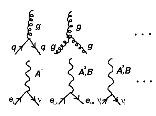
Figure 1: Some Feynman rules (=elementary interactions) of the “gauge sector”: the quark-gluon coupling, the 3-gluon coupling, and the electroweak couplings of the leptons: charged, and neutral currents. Note the arrows on quark and lepton lines (continuous ones), that correspond to the “flow” of U(1)_Y charges. Also, left fermions remain left, and right ones remain right; this is a consequence of the spin 1 nature of the gauge bosons (wavy lines)

The elementary interactions can be conveniently represented as shown in fig. 1. Each of these plots corresponds to a certain “Feynman rule” (elementary diagram), that are used to calculate the amplitudes of probabilities of the admitted physical processes. For instance, the Feynman rule of the first plot (quark-quark-gluon) tells us the presence of a $g_{3}$ coupling constant, and other factors related to the spin structure, too; it corresponds actually to the term of interaction between $\psi_{a}$ and $A_{\mu}^{B}$ in equation 2. Joining the elementary diagrams in the admitted manners (matching the type of lines) one obtains the list of the possible processes in terms of “Feynman diagrams”. Feynman diagrams are in fact a very convenient manner to organise the actual computation; in the following, however, we will use them mostly to illustrate the content of the theory, and not to perform computations.

All this story of symmetries and interactions is beautiful, but there is an high price to pay for that:

No mass is allowed, exactly due to $G_{321}$ (standard model) gauge invariance!

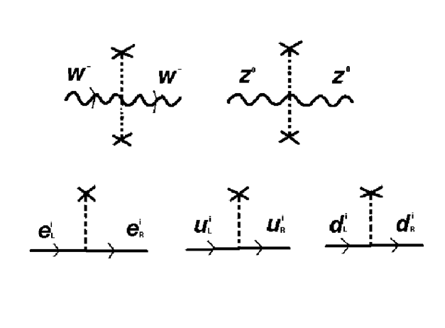
Figure 2: The Higgs particle (dotted line) couples with ordinary particles, and its vacuum expectation value (cross at the end of the dotted line) breaks the electroweak symmetry and generates mass terms. The $g_{1}$ and $g_{2}$ gauge couplings are in the vertices with $W$ and $Z;$ the Yukawa couplings sit in those of quarks and leptons ($i=1,2,3$ is the family index). Here, the arrows illustrate the “flow” of electromagnetic charges, that is conserved; instead, the SU(2)_L or U(1)_Y charges flow into the Higgs boson and gets lost in the vacuum. Similarly, the Higgs particle gets mass via its self-coupling.

1.4 Origin of the masses

Here we come to the second foundation of the SM. The masses arise in a completely particular manner: through a symmetry breaking ascribed to the vacuum [6]. More specifically, it is postulated that a scalar SU(2)_L-doublet exists (the Higgs boson), with hypercharge $-1/2,$ and it obtains a vacuum expectation value:

$$H=\left|\begin{array}[]{c}H^{0}\\ H^{-}\end{array}\right|\ \ \ \ \mbox{ such that }{\rm Re}[H^{0}]\neq 0$$

This hypothesis is not as strange as it might sound, since it is a rather common situation in physics of condensed matter, e.g. a spontaneous magnetisation breaks the rotational symmetry. In consequence of this assumption, the electroweak invariance is lost (only the electric charge symmetry remains untouched), and the $W^{\pm}$ and $Z^{0}$ bosons acquire mass. Also, by introducing 9 new parameters between the Higgs boson and the quarks and leptons (Yukawa couplings), one can account for their masses. See figure 2, and note the left-right structure of the couplings of quarks and leptons (Dirac type mass, like the one in section 1.2). The only communication between different families in the SM arises at this point, and involves only the charged weak currents, To explain this well, it is necessary to go into some subtleties. (1) The particles that have interactions with the $W$ are only the doublets, $q_{L}$ and $l_{L},$ so we have interaction structures like $u_{L}^{i}\to W^{+}d_{L}^{i};$ however, (2) (as we see from fig. 2) the particles with definite mass require to match left and right quark (lepton) states, namely, $d^{i}_{L}$ should match with $d^{i}_{R},$ and similarly for $u$ quarks and charged leptons. So, these two are different prescriptions, or in other terms there is a clash between the “interaction eigenstates” and “mass eigenstates”. Normally, people refer to mass eigenstates (e.g. the top; the electron; etc.); thence charged currents must be non-diagonal (see fig. 3). For leptons, the absence of neutrino masses implies that the non-diagonality is just formal (of no physical significance): e.g. $\nu_{\rm e}$ is by definition the state associated to the electron by charged weak currents.

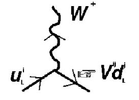
Figure 3: How the charged currents in the SM permit the communication between different families. The symbol indicated by $V$ in the figure is an unitary matrix (named CKM matrix after Cabibbo, Kobayashi and Maskawa [8]) that contains 4 physical parameters: three angles of mixing (like the three Euler angles of an orthogonal matrix) and one complex phase; this latter is the seed of CP-violating phenomena. This delicate sector of the SM will be tested in detail by experiments with bottom- and strange-hadrons (see lecture of Costantini at this Conference)

We are close to the end of the list of parameters, and we must introduce now the self-interaction of the Higgs particle (scalar potential):

$$U=\frac{\lambda}{4}\left(|H|^{2}-v^{2}\right)^{2}$$ (3)

with two parameters, $\lambda$ (the Higgs boson self-coupling) and $v$ (the vacuum expectation value, as it should be clear). Notice that we omitted to list an additive constant; this has no dynamical meaning if gravity is ignored, otherwise, it should be identified as (a contribution to) the vacuum energy, and we know by sure that this is quite small in comparison with the “natural” scale $v^{4}\approx 10^{50}$ GeV/cm³!!! Actually, there are still some more parameters, related to the non-abelian gauge bosons (one for SU(3)_c and one for SU(2)_L) that formally can be written as interaction terms like $\theta\times G_{ab}G_{cd}\epsilon^{abcd}.$ While the one related to SU(2)_L is considered harmless, the one related to SU(3)_c poses serious problems for phenomenology (“strong CP” problem [9]), and thence has to be small. We will not list these in the following, but we have to stress that these are very delicate and mysterious points of the SM; surely they indicate (some of) its frontiers.

1.5 Successes and troubles

Let us summarise the content of the model by some counting. The number of matter fermions for family is 15, 3 leptons, and 4 quarks which come in three types (“colour”). Three families, 45 matter particles. Then there are 9 massless spin 1 bosons (photon and gluons), and three that are massive instead. The number of parameters is

$$18\ (=3\ +\ 9\ +\ 4\ +\ 2).$$

These are all the fundamental parameters that are compatible with the requisite of “renormalizability”. In short, this means “calculability” of the theory; in more diffuse terms, a theory of quantised fields (that represent particles) is termed renormalizable when the quantum fluctuations (referred as “loops”, in connection with their representations by Feynman diagrams) produce relatively harmless infinities, namely only those that can be re-absorbed in the parameters of the theory. So a non-renormalizable theory must be modified to become consistent, for instance:
(1) adding new parameters (no need in the SM–well, apart from three more of them, the $\theta$ parameters and the cosmological constant, that we brutally set to zero);
(2) or new fields (e.g. if only left electrons were to exist, the electromagnetic theory would be inconsistent due to so-called quantum anomalies; a right handed electron cures this problem. More complex is the case of electroweak interactions, but due to a conspiracy of all the particles in a family, no such trouble exists);
(3) or sometimes, it is necessary to reinterpret the theory as a non-fundamental one (e.g. effective 4 fermion interactions result when a virtual $W$ boson is exchanged between two pairs of them; but a 4 fermion fundamental interaction, in itself, would be not renormalizable).
The proof that the SM is renormalizable is not simple, however, gauge invariance turns out to be a crucial ingredient for that [10].

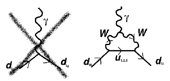
Figure 4: Neither the photon nor the $Z$ bosons are able to change the family ($i\neq j$) at a fundamental level: the first plot–Feynman rule–does not exist in the SM. However this happens at an effective level: second plot and other loop diagrams.

The list of successes of the SM is impressivly long; broadly, can be divided in those related to strong interactions (with few parameters) and those of electroweak interactions (with several parameters). We will limit here to two of them, that are of rather non-trivial nature (for a full account, books and reviews should be consulted):
(1) Electroweak precision measurements
Due to the assumption that the Higgs particle is a doublet, the scalar potential has a special structure, that ensures a relation between the $W$ and $Z$ masses and the gauge couplings of the SU(2)_L and U(1)_Y groups ($g_{2}$ and $g_{1}$) at the lowest order:

$$\frac{M_{W}^{2}}{M_{Z}^{2}}=\frac{1}{1+(g_{1}/g_{2})^{2}}$$ (4)

this relation would not hold, for instance, if the Higgs boson were in the “triplet” representations of SU(2)${}_{L}.$ This argument suggests that the hypothesis of “doublets” is correct, at least in first approximation. Actually, there are calculable corrections to this relation due to “loop” effects, which increase the left-hand side by:

$$\rho=1+\frac{3}{4}\frac{g_{2}^{2}}{(4\pi)^{2}}\times\frac{m_{top}^{2}}{M_{W}^{2}}+\mbox{smaller terms;}$$ (5)

$(4\pi)^{2}$ is the typical loop factor. These calculations have been first made by Veltman [11]; the predictions have been verified at LEP and other experiments (see for instance the reviews in [4]). What we want to emphasise is that a new parameter, the top mass, enters into the game, so that precise measurements of $M_{W},$ $M_{Z}$ and of the coupling constants give informations on the top mass, even if we were to ignore that the top quark existed . Similarly, by this method it is possible to get some information on the Higgs boson mass. The sensitivity is only logarithmic, much weaker than the one to the top mass, however present data are precise enough to show an indication for a relatively light Higgs boson (assuming that this is the only new particle that contributes).
(2) Neutral currents
As we saw, in the SM it is possible to change the family only at the price of emitting a charged spin 1 boson (fig. 3). However, by a combination of two charged currents, it is possible to have an effective neutral current transition with change of family. The diagram shown in fig. 4 gives in fact an amplitude for electromagnetic dipole transition, with a dipole $D$ of the size

$$D(d_{i}\to d_{j}\gamma)=V_{ki}^{*}V_{kj}\times\frac{eg_{2}^{2}}{(4\pi)^{2}}\times\frac{m_{d_{i}}}{M_{W}^{2}}\times f\!\!\left(\frac{m_{u_{k}}^{2}}{M_{W}^{2}}\right)\ \ \ \ \mbox{where }i\neq j$$ (6)

($f$ is an adimensional loop function [12]). Beside the crucial electroweak ingredient, to obtain the correct quantitative estimate it is necessary to consider gluonic corrections [13]; so, it is rather remarkable such a transition ($b\to s\gamma$) has been observed, and with a rate that agrees with the one predicted in the SM.

The SM has also some weak points; we saw the large number of parameters, the undetected Higgs particle (that will be discussed further later on), and the replica of the fermions in three families should be added to the list. But the fatal failure seems to be the following one: Neutrinos are predicted to be massless, while experiments operated in underground sites suggest that they are massive [14]. This rigidity of the SM is due to the global symmetries it has: A strict conservation of the total number of quarks (equivalent to the “baryon number” $B$); and also of the number of leptons of each family (conservation of the “family lepton numbers” $L_{{\rm e},\mu,\tau},$ the sum being called the lepton number $L$). In the language of Feynman diagrams, this means that quark lines are not turned into lepton lines (or viceversa); and that the arrows in the fermionic lines never clash. The problem of massive neutrinos is very urgent in our view, and will be discussed further in the following.

However, another very evident (and, perhaps, deeper) limitation of the standard model of elementary particles is that gravity is not included. This has to do with the fact that quantising gravity turned out to be a very difficult problem. Anyhow, it is rather reasonable to think that the model of elementary particle would look rather different at the Planck scale $(\hbar c/G_{Newton})^{1/2}\approx 1.2\times 10^{19}$ GeV. There are ideas on how to search for manifestations of quantum gravity by using ultra-high energy cosmic rays; also, one imagines that a proper understanding of black holes would require to make further steps toward a full theory of gravity. The concerns regarding the status of the cosmological constant stem from similar considerations.

2 Modifying the standard model

In the following, we focus on massive neutrinos [14], in consideration of the urgent character of the problem they pose for the SM, and also because certain reasonable answers can be offered. After a first harsh (“phenomenological”) approach, we will consider more refined and satisfying (“theoretical”) answers; ideas like existence of “right-handed” neutrinos, “quark-lepton symmetry” and “grand unification” will be introduced. At the end, we will come back to Higgs particle and to related arguments for supersymmetry at the weak scale.

2.1 A harsh way to massive neutrinos

It is not possible to introduce masses of neutrinos in the SM. However, it is possible to write neutrino masses with 2-spinors only; instead than the usual structure $q_{R}\to q_{L},$ one can use $\overline{\nu_{L}}\to\nu_{L},$ in the sense that the role of the right state can be played by the anti-neutrino: This is what is called Majorana mass. (For reappraisal, one sees that this step is forbidden, unless one admits that the symmetry U(1)_Y is violated, since particles and anti-particles have opposite charge—with Feynman diagrams, one says that this mass term produces clashing arrows). Here, we postpone the problem of theoretical justification, and simply assume the existence of Majorana neutrino mass terms. These can be arranged in a mass matrix ${\cal M},$ which is symmetric, and thence can be decomposed as follows:

$${\cal M}_{\ell\ell^{\prime}}=\sum_{j=1,2,3}U_{\ell j}^{*}\ m_{j}\ \exp(i\xi_{j})\ U_{\ell^{\prime}j}^{*}\ \ \ \ \ell,\ell^{\prime}={\rm e},\mu,\tau$$ (7)

$m_{j}$ are the three neutrino masses; $U_{\ell j}$ is the MNS (after Maki, Nakagawa and Sakata [16]) unitary mixing matrix, analogous to the CKM matrix (and with the same number of physical parameters); and $\xi_{j}$ are the so-called “Majorana” phases (two of them having physical meaning). All in all, we have 9 new physical parameters.

2.1.1 What do we know on massive neutrinos?

Now we have to face the question; What is actually known from neutrino experiments? As reviewed by Kajita and Stanev in this conference, there is evidence that neutrinos oscillate, as suggested by Pontecorvo [17]. The relevant experiments can be conceptualised in three main steps; the production of a neutrino state, its propagation, and finally its detection. The states produced and detected are the “interaction eigenstates”, that however need not coincide with the “mass”, or more in general with the “propagation eigenstates”. In more precise terms, a neutrino generated by weak interactions (say, a $\nu_{\mu},$ tagged by a $\mu$ produced in association) is supposed to be a superposition of propagation eigenstates, $\nu_{1,2,3}$; if the masses of neutrinos are different, these states propagate differently; thence, a subsequent detector could reveal a disappearance of the original neutrino $\nu_{\mu}$ (or the appearance of a new type neutrino, say $\nu_{\tau}$). This is described by probabilities of survival (or of conversion) whose entities depend on the neutrino mixing and the differences of masses squared. So: (1) atmospheric neutrinos inform us on one squared mass difference and one mixing angle (these results can be regarded as indication of $\nu_{\mu}$ disappearance; Super-Kamiokande gives also indications of $\nu_{\tau}$ appearance via neutral currents events); (2) solar neutrinos inform us on another (squared) mass difference and another mixing angle (this results can be regarded as $\nu_{\rm e}$ disappearance; neutral current signals can be seen by Super-Kamiokande and SNO detectors together). So, there are 5 parameters that are simply unknown at present. They are

1. the mixing between $\nu_{\rm e}$ and the state responsible of atmospheric oscillations, $|U_{{\rm e}3}|;$

2. a phase that can cause CP violating oscillations (included in $U_{\ell i}$);

3. the mass of the lightest neutrino;

4. the Majorana phases $\xi_{j}.$

We have plenty of choice of what to study next! However, difficulties are not lacking, too…

2.1.2 Can we measure something more?

Let us discuss the parameters of the previous list.

(1) The first parameter is bound by the CHOOZ experiment to be small, $|U_{{\rm e}3}|^{2}<2.5\times 10^{-2}$ (actually, the bound depends to a certain extent on the mass differences). In fact, there are some theoretical arguments suggesting that this parameter is even smaller, at the level of $|U_{{\rm e}3}|^{2}\sim 10^{-3};$ these will be discussed in section 2.2.3. So, the effects on oscillation probabilities could be quite tiny and would be not possibly found even after refining cosmic ray neutrino experiments. Actually, it seems rather difficult that present generation of long-baseline experiments will achieve sensitivity to such a small value (compare with the report of Scapparone for this Conference). A completely different possibilities is offered by the detection of a type-II supernova, since the neutrino burst are substantially affected by the presence of even such a small value of $|U_{{\rm e}3}|$ [18].

(2) As for the CP violating phase, it is rather difficult to foresee the perspectives of measurement at the present stage. It seems to us that success could be possible only if the solar neutrino problem has relatively large values of the mass difference (“large angle Mikheyev-Smirnov-Wolfenstein” solution [19]–see contribution of Kajita); this possibility could be tested by the KamLAND experiment which aims at detecting neutrinos from distant reactors.

(3) The most sensitive tool to the lightest neutrino mass is the search of anomalies in the endpoint spectra of $\beta$ (=electron) emitters with low $Q$-value, since in that kinematical regime the mass of the neutrino emitted in association becomes relevant. The experimental searches (Troitsk, Mainz) bound the mass of this neutrino to be below the few eV range (theoretically, it is not excluded that the actual value is close to this one; in that case, however, oscillation experiments would force the conclusion that the spectrum is almost degenerate, which does not sound particularly appealing). Note that close type-II supernovas could give some information on this parameter, too. Also, cosmological considerations give valuable information on massive neutrinos as sub-dominant components of the Universe (assuming of course that the main components and the dynamics are well understood), since the big-bang picture suggests the existence of a sea of relic neutrinos, a close relative of the cosmic microwave (photon) background. In passing, we have to say that it is very hard to conceive other (non-gravitational) tests of the relic neutrinos hypothesis.

(4) The Majorana phases are very-very difficult to measure directly. Actually, the only handle of which we are aware is a rather indirect one, namely a measurement of these parameters in combination with other ones, which could be possible observing the neutrinoless-$2\beta$ decay (see fig. 5). In this transition, a nucleus increases its charge by two unities, by emitting two electrons simultaneously. If detected, this transition could inform us on the size of $|{\cal M}_{\rm ee}|^{2},$ which depends also on the Majorana phases. The uncertainties in the description of nuclear effects could limit quantitatively the precision of our inferences; however, a detection of this transition would be of great significance, since it would strongly suggest that neutrino have Majorana type mass: oscillation experiments cannot help do this. The present limit on $|{\cal M}_{\rm ee}|$ has been obtained by the Heidelberg-Moscow Collaboration and is in the $0.1-1$ eV range.

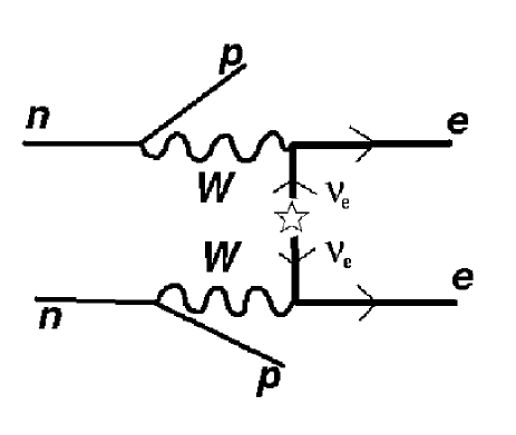
Figure 5: Diagram for neutrinoless-$2\beta$ decay at level of nucleons ($n,$ $p$ are neutrons and protons). Note the clashing arrows in the the neutrino lines, that are characteristic of the Majorana mass of neutrinos, and signal the violation of the lepton number.

However, even in the optimistic assumption all the unknown quantities we discussed will be measured, it is evident that one of the parameters of the neutrino mass matrix will remain unmeasured ($5-4=1$).

2.2 A kind way to massive neutrinos

Now, we discuss some (theoretically) respectable extensions of the standard model, with massive neutrinos and in general with new physics.

2.2.1 Adding new particles

We start considering the Higgs boson $H$ and the left-leptons $l_{L}$, that have the same gauge numbers, $|1,2,-1/2|$ (notation as in table 1). An admitted interaction must be invariant, so the product $l_{L}H^{*}$ seems to be OK. But it is the space-time structure that is not OK, since combining a spinor and a scalar we do not obtain an invariant. One simple solution is to introduce a new fermion $\nu_{R},$ with no gauge numbers, and construct $l_{L}H^{*}\overline{\nu_{R}}.$ The answer we get is rather obvious: we just introduced something that must be called “right-handed” neutrino, and we obtained a Yukawa interaction completely analogous with quark or charged leptons Yukawa terms (this term alone would originate what is called a Dirac mass for neutrinos). But we learned that $\nu_{R}$ has no gauge interactions, so for consistence we must consider the invariant $\nu_{R}\nu_{R},$ too (=Majorana mass for the right-handed neutrino). These two elements give rise to the famous “see-saw” model for the masses of the left-neutrinos [21] (which is Majorana in type; the name comes from the fact that, the more the right-handed neutrino masses go up, the more the left-neutrino masses go down): see fig. 6.

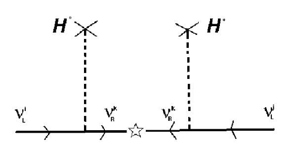
Figure 6: Diagram for the see-saw neutrino masses. The right-handed neutrinos are supposed to be heavy, and act only as quantum fluctuations. However, they introduce a new ingredient, the violation of the lepton number (testified by the clashing arrows). Instead, the U(1)_Y charge flows in the vacuum through the Higgs boson lines.

It should be noted that, even if the right-handed neutrino has super-heavy mass and cannot be produced at accelerators, it still leaves its footprints in the masses of left-neutrinos. The generated mass can be regarded effectively as a $(l_{L}H^{*})^{2}$ term; it reveals its non-fundamental nature from the fact that it is not renormalizable (one can draw here a very close analogy with the 4 fermion weak interactions). Note that the number of parameters is still enlarged! However, some of these parameters might have some interesting manifestations, for instance they can generate a leptonic asymmetry in the early Universe [22].

There is at least one alternative possibility that we feel should be mentioned: if, in order to obtain Majorana masses for neutrinos, we directly multiply two leptonic doublets, we find the quantum numbers $|1,3+1,-1|.$ Thence, by postulating a triplet scalar $\Delta$ with U(1)_Y charge $-1,$ we can construct the invariant term $l_{L}l_{L}\Delta;$ and if we give a tiny (see eq. 5 and discussion therein) vacuum expectation value to the neutral component of the triplet, we find again Majorana masses. So, the question arises, which of these (or other) mechanism for massive neutrinos is the correct one? This is very difficult to answer convincingly, and it could be considered a frontier of the “theory beyond the SM”!

2.2.2 Larger gauge groups

We proceed in the presentation of promising ideas, and pass to the concept of grand unification [23]. The existence of right-handed neutrinos–whose interest has been already discussed–can be argued on the basis of quark-lepton symmetric spectrum (even if the Majorana mass of the right-handed neutrinos is by itself a point of asymmetry). This hypothesis becomes compulsory if we assume that the SM is a group of residual symmetry of certain “unification groups.” We just present few examples and limit ourselves to illustrate how the matter fermions (and the right-handed neutrinos) fit in the representations of larger groups:
SU(5). (Georgi-Glashow) This group of $5\times 5$ matrices obviously includes SU(3)_c and SU(2)_L as the upper $3\times 3$ and lower $2\times 2$ blocks, while U(1)_Y is in the diagonal. The representations where the matter fermions sit are:

$${\bf 10=}\left|\begin{array}[]{ccccc}0&\overline{u_{R3}}&-\overline{u_{R2}}&{u_{L1}}&d_{L1}\\ &0&\overline{u_{R1}}&{u_{L2}}&d_{L2}\\ &&0&{u_{L3}}&d_{L3}\\ &&&0&\overline{{\rm e}_{R}}\\ &&&&0\end{array}\right|\ \ \ \ \ {\bf\bar{5}=}\left|\begin{array}[]{c}\overline{d_{R1}}\\ \overline{d_{R2}}\\ \overline{d_{R3}}\\ \nu_{L}\\ {\rm e}_{L}\end{array}\right|\ \ \ \ \ {\bf 1=}\ \nu_{R}$$ (8)

(1,2,3 are the index of SU(3)${}_{c};$ the 10 matrix is antisymmetric). In this context, the right-handed neutrino has the same status as in the SM.
SU(4)$\times$SU(2)${}_{L}\times$SU(2)_R (Pati-Salam). This group is very satisfying as for the quark-lepton symmetry. The fermions are assigned to:

$${\bf|4,2,1|=}\left|\begin{array}[]{cccc}u_{L1}&u_{L2}&u_{L3}&\nu_{L}\\ d_{L1}&d_{L2}&d_{L3}&{\rm e}_{L}\end{array}\right|\ \ \ \ \ \ {\bf|4,1,2|=}\left|\begin{array}[]{cccc}u_{R1}&u_{R2}&u_{R3}&\nu_{R}\\ d_{R1}&d_{R2}&d_{R3}&{\rm e}_{R}\end{array}\right|$$ (9)

(note the presence of right-handed neutrinos). Leptons, in a sense, are just the fourth type of quarks. For us is difficult to see this, and maintain the opinion that it has no meaning. One could consider a weak point of this assumption the fact that there are three different (non-unified) gauge subgroups (however, by imposing a parity that relates $L$- and $R$-subgroups this improves).
SO(10) (Georgi, Fritzsch-Minkowski). This group includes SU(5) (since a complex 5 vector can be obviously mapped in a real 10 vector) but also the Pati-Salam group (since SO(6)$\sim$SU(4)). Each family of matter fermions sits in a single representation:

$${\bf 16=10+\bar{5}+1=|4,2,1|+|4,1,2|}$$ (10)

Like SU(5), this group has an unique coupling. However, the breaking of SO(10) down to the SM might take place in several steps (with several “intermediate” scales).

Whatever the gauge group, it is needed that the large gauge symmetries are broken (and also that the fermion masses are generated). This calls for scalars, and opens up many possibilities (and troubles, see section 2.3). We mention only one specific point here [24]. As we saw, the SO(10) or Pati-Salam group naturally includes right-handed neutrinos, which is certainly a good thing. However, the reduction of SU(2)_R symmetry typically requires the existence of scalar “right” triplets; the symmetry forces the existence of “left” triplets; so that, there are two competing sources for massive neutrinos: see-saw and “left” triplet.

Apart from neutrino masses, the unification groups have (some) predictivity on the unification of gauge couplings, of fermion masses, and also on proton decay. From the experimental point of view, the last aspect is surely the most interesting. Proton decay could be due to the new gauge bosons of the grand unified group, that permit communication between quarks and leptons; however there are also other possibilities, e.g. new scalar particles might have an important role (this happens commonly in supersymmetric models). Trying to summarise in a few words the present situation: proton decay is not experimentally found (strongest limits come from the Super-Kamiokande experiment) but there are some theoretical models that offer hopes of detection for future detectors (new detectors like ICARUS have superior properties, but its mass might limit its discovery potential … should a Mega-Kamiokande be built?). Experimental and theoretical proposals, however, are still at a stage of discussion; the “future” seems not close.

2.2.3 Use of quark-lepton symmetry

Here, we present an ansatz for massive neutrinos, that we consider quite reasonable since it is based on a principle: quark-lepton symmetry (or more precisely, quark-lepton correspondence). One starts to note that the masses of up-type quarks increase strongly changing family, in comparison with what happens for down type quarks, or also for charged leptons. This difference of hierarchies motivate the assumption that neutrinos have still weaker differences among them. An actual implementation of this idea, due to Sato and Yanagida [25], is the assumption that the neutrino mass has the structure:

$${\cal M}\propto\left|\begin{array}[]{ccc}\varepsilon^{2}&\varepsilon&\varepsilon\\ &1&1\\ &&1\end{array}\right|\ \ \ \ \ \varepsilon=1/20\sim\sin^{2}\!\theta_{C}\sim m_{\mu}/m_{\tau}$$ (11)

(where the Cabibbo angle $\theta_{C}$ is a parameter of the CKM matrix). To make the statement sufficiently vague (or equivalently, sufficiently precise) one postulates that the elements of the matrix include also coefficients order unity (these are in fact are essential in order to generate three different neutrino masses).
The weak points of this assumption are that:
(1) the overall scale is not predicted;
(2) the hierarchy of masses between the two heavier neutrinos tends to be rather weak.
The advantages (after the weak points are made up, by adjusting the unknown “coefficients” and the overall scale) are that:
(1) a large mixing for atmospheric neutrinos is automatic;
(2) there is a prediction of “large angle Mikheyev-Smirnov-Wolfenstein” solution (with the correct type of mass hierarchy);
(3) the value of $U_{{\rm e}3}$ is predicted to be small.
Note, incidentally, that also neutrinoless $2\beta$ transitions are predicted to be suppressed, since $|{\cal M}_{\rm ee}|^{2}\sim\Delta m^{2}_{atm}\times\epsilon^{4}.$ This is essentially a manifestation of the fact that neutrinos are supposed to obey a sort of family hierarchy, and is tightly related to the suppression of $U_{{\rm e}3},$ since $U_{{\rm e}3}\sim\epsilon.$

2.3 Troubles with fundamental scalars, and supersymmetry as solution

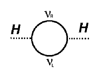
Figure 7: An example of quantum communication (loop diagram) between hypothetical heavy mass scales–right-handed neutrino in this example–and the electroweak–Higgs–mass scale.

Here we come to one trouble of the SM (even more severe in the unified theories). This is, in essence, a problem of hierarchy of scales [26]. One can say that, due to quantum fluctuations, heavy masses creep in the Higgs boson ($\sim$ weak boson) scale and want to destabilise it. For instance, the diagram in the fig. 7 changes the coefficient of the bilinear term $\mu^{2}\times|H|^{2}$ by an amount of the order of

$$\delta\mu^{2}\sim\frac{Y^{2}}{(4\pi)^{2}}\times M_{\nu_{R}}^{2}\ \ \ \ \mbox{ where }\ \ \ \ \left\{\begin{array}[]{l}Y=\mbox{{\sc Yukawa} coupling of neutrinos,}\\ M_{\nu_{R}}=\mbox{Mass of right-neutrinos.}\end{array}\right.$$ (12)

which (apart for the loop pre-factor) seems to produce a huge scale, comparable to $M_{\nu_{R}}$ (not of the order of the electroweak scale as we need). To be picky, one can say that the individual contributions to $\mu^{2}$ are not separately measured; that only their sum has physical meaning; and that we should not ask the theory to say more than it can. However, in this manner we would most probably give up any chance of predicting these fundamental parameters, since a hypothetical (more complete) theory would be forced to explain a very precise fine-tuning. This situation motivated several extensions of the SM, and all of them have new physics (close) at the electroweak scale; for instance, it was postulated that the Higgs particle is not fundamental—but instead a pion-like object (technicolor).

We will concentrate the discussion on supersymmetric models [27]. Supersymmetry is an extension of the space-time group, which relates fermions and bosons by a symmetry transformation. In the models that could be possibly relevant for electroweak scale physics, supersymmetry commutes (=is unrelated) with the gauge group; so that any ordinary particle obtains a “partner”, and we have scalar electrons (sleptons), fermionic gluon (gluino), etc. Actually, it is necessary that the number of Higgs doublets is at least two. We recommend to make reference to the contributions of Ganis and Denegri for a more detailed description of these models, and discussion of the perspectives of confirmation. The connection with the “hierarchy problem” is due to an amazing property of supersymmetry as a quantum field theory: that the “loops” involving bosons and fermions compensate each other, and contributions like those in eq. 12 do not arise. At this point, however, we have to recall that an extension of the SM should have broken supersymmetry in order to be realistic (otherwise, for instance, the “partners” would have the same mass of the ordinary particles). The actual mechanism for supersymmetry breaking is an open question at present, which surely is not a nice feature, even if there are reasonable proposals. However, if one assumes that the breaking scale is order of the TeV, and restricts the allowed breaking terms to so-called “soft-breaking”, the quantum properties are maintained and the hierarchy problem is under control. In this paragraph, we presented an instant summary of the idea of “supersymmetry at the weak scale”. Much more could be said, however, the key question that we have to answer is: Do these considerations have any relevance to the description of Nature? Let us list three considerations that suggest (but not “imply”) an affirmative answer:

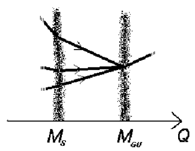
Figure 8: Sketchy plot of the unification of SM gauge couplings in supersymmetric context. The two vertical bands indicate where supersymmetry begins (scale $M_{S}$) and where the unified dynamics begins (scale $M_{GU}$); they are sources of uncertainties for the predictions.

• Electroweak precision measurements suggest the existence of a light Higgs particle as predicted in (minimal) supersymmetric extensions of the standard model.
  The prediction is mainly due to the fact that the Higgs boson self-coupling $\lambda$ in eq. 3 turns out to be a combination of the (measured) electroweak gauge constants (the scalar potential is quite constrained in these models). This prediction can be tested at future colliders (… or if we are really lucky, even before; see Denegri, these Proceedings).

• Gauge couplings unify in the context of low energy supersymmetric model.
  Here we mean that: the extrapolation of the couplings is compatible with the hypothesis of grand unified dynamics (broken below a certain scale $M_{GU},$ see fig. 8) [28]. This does not happen in the ordinary SM (not within a model with a single scale of breaking). It is rather remarkable that the large unification scale, $M_{GU}\sim 2\times 10^{16}$ GeV, is comparable with what is suggested by a see-saw mechanism for massive neutrinos. Can proton decay provide the crucial confirmation of this indication? Specific channels exist [29], like

  $$p\to K^{+}\bar{\nu};$$ (13)

  the presence of a kaon (the characteristic aspect) results from the fact that proton decay is expected to be due to Yukawa type interactions, and to observe for this reason the family hierarchy (see fig. 9). However, the dependence on the unknown aspects of the model is strong (and no doubt that the usual Yukawa sector already challenges our understanding), and, theoretically, it is not excluded that the proton decay process is rather suppressed.

  

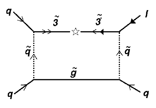
  Figure 9: One diagram for supersymmetric proton decay. $\tilde{q}$ and $\tilde{g}$ are the supersymmetric partners of the quarks and gluons; instead, the SU(3)_c triplets $\tilde{\em 3}$ and $\tilde{\em 3}^{c}$ are fermions, that are paired by grand unification with the supersymmetric partners of the Higgs particles. The open arrows indicate the flow of baryon number, the closed ones the flow of lepton number; the star is the point of clash.

• A cold dark matter candidate exists.
  The lightest supersymmetric particle (LSP) is stable due a discrete symmetry that can be incorporated in the model (which, for the record, is called R parity). Is the galactic “LSP cloud” [30] responsible of the modulated signal seen in the DAMA experiment shown by Incichitti at this Conference? If this were true, this result would be of enormous importance, not only for the direct detection of dark matter but also as a first signal of “supersymmetry at the electroweak scale”; and it would also open quite interesting perspectives for future collider searches, as discussed by Ganis. Further studies and confirmations are of essential importance (Incichitti).

We would like to add a comment on the Higgs boson mass. A value on the large side (say, $>120$ GeV) would indicate in a supersymmetric context a rather strong hierarchy between the vacuum expectation values of the two Higgs doublets, $\langle H_{up}^{0}\rangle\gg\langle H_{down}^{0}\rangle.$ This would suggest an entire series of theoretical and phenomenological questions; for example, the (Yukawa type) proton decay is expected to be enhanced in this regime. Instead, if the Higgs boson mass turns out to be really large (say, $>150$ GeV) it seems not easy to avoid the conclusion that “supersymmetry at the electroweak scale” is in trouble; this will be the crucial test of the model. Finally, we remind that in the SM there is a limit on the Higgs boson mass suggested by the consideration that the self-coupling $\lambda$ should be not driven negative as an effect of the quantum fluctuations, (“vacuum stability” [31]) at least up to the Planck scale where new effects most probably appear. It is rather funny, but this lower limit almost coincides with the upper limit in the (minimal) supersymmetric extension of the standard model. So (if a joke is permitted) we present a prediction for LHC:

$$m_{H}=135\pm 5\mbox{\ GeV}$$ (14)

the reason is that this value will increase the entropy in the minds of several theorists. Note, however, that the decay of a standard and supersymmetric Higgs particles with the same mass (or also the production rate–“cross-sections”) could be rather different; thence, these measurements would offer a possibility to distinguish between the SM and its supersymmetric extension even in this tricky case.

3 (Not quite a) conclusion

We would like to close this pages by spending few words of caution, to remind that failures of the standard model have been often claimed in the past years (today, several of them are considered dubious or simply wrong tracks). Here is an arbitrary selection:

$$\begin{array}[]{lcl}\mbox{\sc THEORETICAL}&&\mbox{\sc EXPERIMENTAL}\\ \mbox{\sc INTERPRETATION}&&\mbox{\sc ANOMALY}\\ &&\\ \mbox{leptoquark}&................................&\mbox{High $x$ and $Q^{2}$ events at {\sc HERA}}\\ \mbox{compositeness}&................................&\mbox{Excess of 4-jet events at {\sc ALEPH}}\\ \mbox{light gravitino}&................................&\mbox{${\rm ee}\gamma\gamma E\!\!\!\!/$\ \ event at {\sc CDF}}\\ \mbox{17 keV neutrino}&................................&\mbox{bump in $\beta$ spectra ({\sc Simpson, ...})}\\ \mbox{monopole}&................................&\mbox{induced currents ({\sc Cabrera})}\\ \mbox{proton decay}&................................&\mbox{contained multitrack events at {\sc KGF}}\\ \mbox{...}&................................&\mbox{...}\end{array}$$

Is there any moral behind these stories? Maybe not; however:
1) they suggest to go slowly and carefully from data to theories and back (because of possible pitfalls of interpretation, of suggestion, etc.);
2) they witness how hard is to reach the frontiers of standard model; and, also, how strong is the desire of particle physicists to find them!

I am grateful to the Organizers and Partecipants (in particular to B. Alessandro, R. Bandiera, P. Blasi, S. Colafrancesco, F. Giovannelli, A. Grillo, G. Mannocchi, R. Ramelli, P.G. Rancoita, E. Scapparone, A. Stamerra, A. Surdo) for the most pleasant and informative discussions, and to F. Cavanna for a careful reading of the manuscript. I would like to take this occasion to thank R. Barbieri, V. Berezinksy, S. Bertolini, W. Buchmüller, A. Di Giacomo, A. Masiero, N. Paver, S. Petcov, E. Roulet, G. Senjanović, A.Yu. Smirnov, M. Veltman and T. Yanagida to whom I owe what I know on the SM and its extensions, and who largely deserve the credit for niceties in the presentation; errors and misinterpretations of course are mine.

References

- [1] S.L. Glashow, Nucl. Phys. 22, 579 (1961); S. Weinberg, Phys. Rev. Lett. 19, 1264 (1967); A. Salam, Proceedings of the Nobel symposium held 1968 at Lerum, Sweden, Stockholm 1968, 367-377 (Nobel prize 1979 for physics).
- [2] Some reference texts: L.B. Okun, “Leptons and quarks,” Amsterdam, Netherlands: North-Holland ( 1982) and F. Halzen and A.D. Martin, “Quarks and leptons: An introductory course in modern particle physics,” New York, Usa: Wiley ( 1984) they are complemented well by L.H. Ryder, “Quantum Field Theory,” Cambridge, UK: Univ. Press ( 1985). A recent useful review: Zoltan Kunszt, “Bread and butter standard model,” hep-ph/0004103.
- [3] Historical and conceptual accounts are presented in the book “The rise of the standard model” edited by L.M. Hoddeson, L. Brown, M. Riordan and M. Dresden (based on a conference held in 92 in Stanford). See also G. ’t Hooft, “The glorious days of physics: Renormalization of gauge theories,” hep-th/9812203.
- [4] Most recent item is: C. Caso et al, The European Physical Journal C3 1 (1998); the material is updated at the web site: http://pdg.lbl.gov/. This is a repository of data and informations of primary importance, and includes reviews for several relevant topics.
- [5] C.N. Yang and R.L. Mills, Phys. Rev. 96, 191 (1954); Phys. Rev. 95 (1954) 631. See also the recent review work L. O’Raifeartaigh and N. Straumann, “Gauge theory: Historical origins and some modern developments,” Rev. Mod. Phys. 72, 1 (2000).
- [6] P.W. Higgs, Phys. Rev. Lett. 13, 508 (1964); Phys. Lett. 12, 132 (1964); Phys. Rev. 145, 1156 (1966).
- [7] Y. Nambu, Phys. Rev. Lett. 4, 380 (1960); Y. Nambu and G. Jona-Lasinio, Phys. Rev. 122, 345 (1961); Phys. Rev. 124, 246 (1961).
- [8] N. Cabibbo, Phys. Rev. Lett. 10, 531 (1963) and ref’s therein; M. Kobayashi and T. Maskawa, Prog. Theor. Phys. 49, 652 (1973).
- [9] C.G. Callan, R.F. Dashen and D.J. Gross, Phys. Lett. B63, 334 (1976); R. Jackiw and C. Rebbi, Phys. Rev. Lett. 37, 172 (1976).
- [10] M. Veltman, Nucl. Phys. B7, 637 (1968); G. ’t Hooft, ibidem, B35, 167 (1971); G. ’t Hooft and M. Veltman, ibidem, B44, 189 (1972) and ibidem, B50, 318 (1972) (Nobel prize 1999 for physics).
- [11] M. Veltman, Nucl. Phys. B123, 89 (1977); Acta Phys. Polon. B8, 475 (1977).
- [12] E.P. Shabalin, Sov. J. Nucl. Phys. 32, 129 (1980); T. Inami and C.S. Lim, Prog. Theor. Phys. 65, 297 (1981); Erratum ibidem, page 1772.
- [13] The large size of the gluonic corrections was first estimated in: S. Bertolini, F. Borzumati and A. Masiero, Phys. Rev. Lett. 59, 180 (1987) and N.G. Deshpande, P. Lo, J. Trampetic, G. Eilam and P. Singer, Phys. Rev. Lett. 59, 183 (1987) The experimental confirmations of the predictions were obtained by the CLEO Collaboration (see [4]).
- [14] We recommend to make reference to the talks of Kajita, Satta, Scapparone, Stanev, Surdo and to [4]. Since neutrino physics is in rather rapid evolution, we believe that it could be convenient to use internet facilities like “The neutrino oscillation industry” (http://www.hep.anl.gov/ndk/hypertext/nuindustry.html). There, it is possible to find informations on many relevant experiments, and other useful “links”.
- [15] G. ’t Hooft, Phys. Rev. Lett. 37, 8 (1976).
- [16] Z. Maki, M. Nakagawa and S. Sakata, Prog. Theor. Phys. 28 870 (1962).
- [17] B. Pontecorvo, Zh. Eksp. Teor. Fiz. 33 549 (1957), where the concept of neutrino oscillations was introduced, by analogy with kaon oscillations. See also [16] and V.N. Gribov and B. Pontecorvo, Phys. Lett. B28 493 (1969).
- [18] A.S. Dighe and A.Yu. Smirnov, “Identifying the neutrino mass spectrum from the neutrino burst from a supernova,” hep-ph/9907423.
- [19] L. Wolfenstein, Phys. Rev. D17 (1978) 2369; S. Mikheyev and A.Yu. Smirnov, Yad. Fiz. 42 (1985) 913, Nuovo Cimento 9C (1986) 17.
- [20] S. Weinberg, Phys. Rev. Lett. 43, 1566 (1979).
- [21] T. Yanagida, in “Proceeding of the workshop on unified theory and baryon number in the Universe”, KEK, March 1979, eds. O. Sawada and A. Sugamoto; M. Gell-Mann, P. Ramond and R. Slansky, in “Supergravity”, Stony Brook, Sept 1979, eds. D. Freedman and P. van Nieuwenhuizen. See also [20] and Georgi and Nanopoulos, as quoted there.
- [22] M. Fukugita and T. Yanagida, Phys. Lett. B174, 45 (1986).
- [23] H. Georgi and S.L. Glashow, Phys. Rev. Lett. 32, 438 (1974); J.C. Pati and A. Salam, Phys. Rev. D10, 275 (1974); H. Georgi, In Coral Gables 1975, proceedings, Theories and experiments in high energy physics, New York 1975, 329-339 and H. Fritzsch and P. Minkowski, Annals Phys. 93, 193 (1975).
- [24] R.N. Mohapatra and G. Senjanović, Phys. Rev. D23, 165 (1981), C.S. Aulakh, B. Bajc, A. Melfo, A. Rašin and G. Senjanović, “SO(10) theory of R-parity and neutrino mass,” hep-ph/0004031 and ref’s therein.
- [25] J. Sato and T. Yanagida, Phys. Lett. B430, 127 (1998); a more accurate discussion of the phenomenology and predictions is in F. Vissani, JHEP 9811, 025 (1998). See also W. Buchmuller and T. Yanagida, Phys. Lett. B445, 399 (1999).
- [26] E. Gildener, Phys. Rev. D14, 1667 (1976); G. ’t Hooft, Lecture given at Cargese Summer Inst., Cargese, France, Aug 26 - Sep 8, 1979; R. Barbieri, Riv. Nuovo Cim. 11, 1 (1988).
- [27] H.P. Nilles, Phys. Rept. 110, 1 (1984); M.F. Sohnius, Phys. Rept. 128, 39 (1985); H.J. Müller-Kirsten and A. Wiedemann, “Supersymmetry: An introduction with conceptual and calculational details,” Print-86-0955 (Kaiserslautern).
- [28] M.B. Einhorn and D.R. Jones, Nucl. Phys. B196, 475 (1982); W.J. Marciano and G. Senjanović, Phys. Rev. D25, 3092 (1982).
- [29] S. Weinberg, Phys. Rev. D26, 287 (1982); N. Sakai and T. Yanagida, Nucl. Phys. B197, 533 (1982); S. Dimopoulos, S. Raby and F. Wilczek, Phys. Lett. B112, 133 (1982).
- [30] J. Ellis, J.S. Hagelin, D.V. Nanopoulos, K. Olive and M. Srednicki, Nucl. Phys. B238, 453 (1984).
- [31] N. Cabibbo, L. Maiani, G. Parisi and R. Petronzio, Nucl. Phys. B158, 295 (1979); G. Altarelli and G. Isidori, Phys. Lett. B337, 141 (1994).