UFIFT-HEP-00-17

hep-ph/0007019

Analyzing the ’t Hooft Model on an $x^{+}$-$p^{+}$ Lattice

Joel S. Rozowsky and Charles B. Thorn

Institute for Fundamental Theory
Department of Physics, University of Florida, Gainesville, FL 32611

()

We study the ’t Hooft model (large $N_{c}$ QCD in 2 space-time dimensions) using an improved approach to digitizing the sum of gauge theory Feynman diagrams based on light-cone gauge $A^{+}=0$ and discretized $p^{+}$ and $ix^{+}$. Our purpose is to test the new formalism in a solvable case, with the hope to gain some insight into how it might be usefully applied to the physically interesting case of $4$ dimensional QCD.

1 Introduction

Last year, with Bering we proposed [1] a new method to digitize the sum of planar diagrams selected by ’t Hooft’s $N_{c}\rightarrow\infty$ limit of $SU(N_{c})$ gauge theories [2]. The proposal, based on the light-cone or infinite momentum frame description of the dynamics, involved discretization of both the $p^{+}$ carried by each line of the diagram and the propagation time $\tau=ix^{+}$, as in [3, 4, 5]. But the main advantage of the new version was a coherent prescription for resolving most of the ambiguities due to $p^{+}=0$ divergences that typically plague the light-cone description.

We hope that our formalism will eventually allow an improved understanding of QCD in 4 dimensional space-time. But in this article, we merely wish to test the proposal in the context of the well-understood case of large $N_{c}$ gauge theories in two space-time dimensions, namely the ’t Hooft model [6]. Our purpose is not to unearth new aspects of the model, but rather to see how its well known properties can be obtained from our new discretization.

The physical content of the ’t Hooft model boils down to an integral equation, essentially a Bethe-Salpeter equation [9], that determines the mass spectrum of $q\bar{q}$ mesons. The reason the limit $N_{c}\rightarrow\infty$ reduces to ladder diagrams (albeit with self-energy corrected quark propagators), is that the 2 dimensional gluon is not dynamical (there are no transverse polarizations). Thus, as with any axial gauge, the light-cone gauge $A_{-}=0$ eliminates all gluon self-interactions, so $A_{+}$ can be integrated out inducing an instantaneous Coulomb potential. But the ’t Hooft limit $N_{c}\rightarrow\infty$ further eliminates all quark loops and all non-planar diagrams, leaving only the planar self energy corrections to the quark propagator, and the ladder bare gluon exchanges (Coulomb interaction) between quark anti-quark lines in the singlet $q\bar{q}$ channel. In light-cone parameters the Bethe-Salpeter equation summing these ladder $q\bar{q}$ diagrams simplifies to the single variable ’t Hooft integral equation [6].

$${\cal M}^{2}\varphi(x)=\left({1\over x}+{1\over 1-x}\right)\mu^{2}\varphi(x)-{g_{s}^{2}N_{c}\over 2\pi}P\int_{0}^{1}dy{\varphi(y)-\varphi(x)\over(y-x)^{2}},$$ (1.1)

where the integral is understood to be evaluated by the principal value prescription. The variable $x$ is the fraction carried by the quark of the total $P^{+}$ of the system (the anti-quark carries $P^{+}$ fraction $1-x$). Also ${\cal M}$ is the mass of the meson bound state and $\varphi$ satisfies the boundary conditions, $\varphi(0)=\varphi(1)=0$.

Since the new formalism discretizes $\tau\equiv ix^{+}=ka$ in addition to $p^{+}=lm$, the corresponding simplifications lead to an equation that is not a straightforward discretization of this integral equation. In particular, the continuum limit can be taken in different ways depending on the ratio $T_{0}=m/a$ (which would be infinite for continuous $\tau$), and we want to explore to what extent these different continuum limits lead to the same physics. We shall find that some care must be taken with the setup of the discrete $\tau$ dynamics in order for this to be true. Indeed, a numerical study shows that the most simple-minded treatment leads to a ground state that becomes unstable at moderate ’t Hooft coupling even with relatively small $P^{+}/m\equiv M$ unless the ratio $a/m=1/T_{0}$ is tuned to be sufficiently small (perhaps infinitesimal for large $M$). If this feature were robust, it would cast doubt on any potential utility of the discretization of $\tau$.

To overcome this difficulty, we find it necessary to veto some of the “densest” discretized Feynman diagrams: a quark must be forbidden to emit 2 gluons at immediately successive time steps, with a similar veto on two successive absorptions. With this simple veto (which is prescribed locally in time), we shall show that the continuum limit reduces to the ’t Hooft model provided only that the total $P^{+}$ of the $q\bar{q}$ system is large compared to the discretization unit $m$. In particular it is not necessary that the ratio $T_{0}=m/a$ be large. Keeping $T_{0}$ finite in the continuum limit leads to the ’t Hooft equation with a non-trivial renormalization of the coupling. Because of this effect, it turns out that the effective (renormalized) coupling is small for both large and small bare coupling, reminiscent of strong/weak coupling duality. The strong coupling limit favors the densest diagrams, so vetoing some of the densest ones has a dramatic effect on the strong coupling behavior of the theory. This possibility was anticipated and discussed in [1] in connection with the nature of the fishnet diagrams in higher dimensional space-time.

The rest of the paper is organized as follows. In Section 2 we set up the discretized ’t Hooft model. We analyze it using a single time-step transfer matrix in Section 3 and using a Bethe-Salpeter approach in Section 4. In Section 5 we discuss and implement the veto which allows a satisfactory continuum limit at fixed $T_{0}$. Discussion and concluding remarks are the subject of the final Section.

2 Discretized ’t Hooft Model

The Lagrange density for $SU(N_{c})$ gauge fields coupled to quarks in the fundamental representation is given by

$${\cal L}=-{1\over 4}{\rm Tr}F^{\mu\nu}F_{\mu\nu}+\bar{q}\left[i\gamma\cdot(\partial-igA)-\mu_{0}\right]q,$$ (2.1)

where $F_{\mu\nu}=\partial_{\mu}A_{\nu}-\partial_{\nu}A_{\mu}-ig[A_{\mu},A_{\nu}]$. We remind the reader that the normalization of gauge fields appropriate for matrix fields and dictated by the gluon kinetic term differs by a factor $1/\sqrt{2}$ from the more standard one:

$$-{1\over 4}\sum_{a}F_{a}^{\mu\nu}F_{a\mu\nu}=-{1\over 2}{\rm Tr}F_{s}^{\mu\nu}F_{s\mu\nu},$$

with $F_{s}\equiv\sum_{a}{\lambda_{a}\over 2}F_{a}$. Thus $A_{s}=A/\sqrt{2}$, and we conclude that $g=g_{s}/\sqrt{2}$. In 2 space-time dimensions we choose the representation of $\gamma$ matrices for which the light-like components are

$$\gamma^{+}=\sqrt{2}\left(\begin{array}[]{cc}0&1\\ 0&0\end{array}\right)\qquad\gamma^{-}=\sqrt{2}\left(\begin{array}[]{cc}0&0\\ 1&0\end{array}\right).$$ (2.6)

With this choice the field equation for the upper component of the quark spinor does not involve the “time” derivative and is an equation of constraint relating the upper component, $q_{1}$, to the lower component, $q_{2}$. Working in light-cone gauge ($A_{-}=A^{+}=0$), we can eliminate the upper component in favor of the lower component yielding the light-cone gauge Lagrange density

$${\cal L}=+{1\over 2}{\rm Tr}(\partial_{-}A_{+})^{2}+i{\psi}^{\dagger}\left[\partial_{+}-igA_{+}+{\mu_{0}^{2}\over 2\partial_{-}}\right]\psi,$$ (2.7)

where $\psi=2^{1/4}q_{2}$.

Our discretization of Feynman diagrams is based on the $x^{+}$ representation of each bare propagator

$$D(p^{+},x^{+})=\int{dp^{-}\over 2\pi}\tilde{D}(p^{+},p^{-})e^{-ix^{+}p^{-}}.$$ (2.8)

Performing the $p^{-}$ integral gives the following Feynman rules for the continuum theory

$$D_{\psi}(p^{+},x^{+}) = e^{-ix^{+}\mu_{0}^{2}/2p^{+}}\rightarrow e^{-\tau\mu_{0}^{2}/2p^{+}}$$

$$D_{A}(p^{+},x^{+}) = i{\delta(x^{+})\over{p^{+}}^{2}}\rightarrow-{\delta(\tau)\over{p^{+}}^{2}}$$ (2.9)

$$V_{\psi^{\dagger}\psi A} = ig\rightarrow g,$$

where the arrows indicate the rules to use with imaginary time.

One way to digitize the ’t Hooft equation (1.1) is to put the variables $x,y$ on a grid, which amounts to discrete light-cone quantization [7, 3], where one discretizes the amount of $P^{+}$ each line of the ladder diagram carries in quanta of $m$

$$p^{+}=lm\qquad l=1,2,3,\ldots.$$

One can then focus on a state of the system of interest (in our case a $q\bar{q}$ system) with total $P^{+}=Mm$. The continuum theory is recovered by taking the combined limits $m\rightarrow 0$ and $M\rightarrow\infty$ while keeping $P^{+}=Mm$ fixed. Following [3, 1], in addition to discretizing the $p^{+}$ of each particle, we also discretize imaginary light-cone time, $\tau=ix^{+}=ka$ ($k=1,2,3,\ldots$). This discretization (which also serves as an ultraviolet cutoff) allows the continuum limit to be reached by keeping $T_{0}\equiv m/a$ fixed and taking both $m,a\rightarrow 0$ and $M\rightarrow\infty$ simultaneously. Actually, since the physics of the discretized model depends only on the ratio $m/a$, the continuum limit is nothing but the large $M$ limit, where $M$ measures the total $P^{+}$ of the system state. The conventional continuous time DLCQ approach (see [8] and references therein) corresponds to the special case $T_{0}\rightarrow\infty$.

Discretization of the quark propagator poses no difficulty. However, for the instantaneous interaction induced by integrating out $A_{+}$, we allow for ambiguities as in [1]. The only constraint is that the discretized propagator become that of Eq. 2.9 in the continuum limit. This allows us to spread out the instantaneous interaction away from $\tau=0$ (see [1] for further discussion). Thus the gauge propagator can be expressed as

$$D_{A}(Mm,-ika)=-f_{k}{T_{0}\over M^{2}}\qquad{\rm where}\qquad\sum_{k=1}^{\infty}f_{k}=1.$$ (2.10)

We require that these arbitrary parameters $f_{k}$ rapidly vanish with increasing $k$. Using this discretization, the Feynman rules for the discrete theory are summarized in Fig. 1.

$\begin{array}[c]{c}\psfig{height=36.135pt}\end{array}$	$e^{-k\mu_{0}^{2}/2MT_{0}}$	$\begin{array}[c]{c}\psfig{height=36.135pt}\end{array}$	$-e^{-k\mu_{0}^{2}/2MT_{0}}$	$\begin{array}[c]{c}\psfig{height=36.135pt}\end{array}$	$-f_{k}{T_{0}\over M^{2}}$
$\begin{array}[c]{c}\psfig{height=36.135pt}\quad\psfig{height=36.135pt}\end{array}$		${g\over T_{0}\sqrt{2\pi}}$	$\begin{array}[c]{c}\psfig{height=36.135pt}\quad\psfig{height=36.135pt}\end{array}$		${g\over T_{0}\sqrt{2\pi}}$

Figure 1: Feynman rules for the discretized ’t Hooft model. Discrete light-cone time flows up the page.

For the purposes of this paper we shall not exploit the full generality of the set of $\{f_{k}\}$’s. We restrict attention to the simplest version where the spread out interaction propagates only one unit in light-cone time, this corresponds to setting $f_{1}=1,f_{k>1}=0$. The Feynman rules of Fig. 1 can be further simplified if we absorb the negative sign from the anti-quark propagator into the corresponding vertex factor. We define new parameters

$$\alpha\equiv e^{-\mu_{0}^{2}/2T_{0}}\quad{\rm and}\quad\kappa\equiv{\sqrt{g^{2}N_{c}\over 2\pi T_{0}}}.$$ (2.11)

We also recall that in ’t Hooft’s large $N_{c}$ limit every additional pair of cubic vertices in the ladder sum corresponds to a completed color index loop, which produces a factor $N_{c}$. Thus we shall also absorb a factor of $\sqrt{N_{c}}$ into each vertex. Simply put, all terms in the ladder sum are only dependent on the ’t Hooft coupling $g^{2}N_{c}$. The simplified Feynman rules are presented in Fig. 2.

$\begin{array}[c]{c}\psfig{height=36.135pt}\end{array}$	$\alpha^{k/M}$	$\begin{array}[c]{c}\psfig{height=36.135pt}\end{array}$	$\alpha^{k/M}$	$\begin{array}[c]{c}\psfig{height=36.135pt}\end{array}$	$-{1\over M^{2}}$
$\begin{array}[c]{c}\psfig{height=36.135pt}\quad\psfig{height=36.135pt}\end{array}$		${\kappa}$	$\begin{array}[c]{c}\psfig{height=36.135pt}\quad\psfig{height=36.135pt}\end{array}$		$-{\kappa}$

Figure 2: Simplified discretized Feynman Rules for ’t Hooft model.

3 Single Time-Step Transfer Matrix

Using the Feynman rules of Fig. 2 we can now proceed to set up a transfer matrix which evolves a singlet $q\bar{q}$ system one step forward in $x^{+}$-time. Once the matrix has been determined as a function of the coupling, $\kappa$, solving the eigenvalue problem will yield the bound state energies as functions of coupling. Since the scalar particle which mediates the Coulomb interaction only lives one time-step, any state can have at most two intermediate scalars. Thus for the simplest systems with $P^{+}/m\equiv M=3,4,5,6$ the number of states are $3,7,14,25$ (the number of states is $(M-1)(M^{2}-2M+6)/6$ for general $M$). For illustrative purposes we shall explicitly present the transfer matrix for $M=4$.

For $M=4$ there are 7 states namely:

$$\begin{array}[]{ccccc}|3,1\rangle=b^{\dagger}_{3}d^{\dagger}_{1}|0\rangle,&&|2,2\rangle=b^{\dagger}_{2}d^{\dagger}_{2}|0\rangle,&&|1,3\rangle=b^{\dagger}_{1}d^{\dagger}_{3}|0\rangle,\\[2.84544pt] |2,1,1\rangle=b^{\dagger}_{2}a^{\dagger}_{1}d^{\dagger}_{1}|0\rangle,&&|1,2,1\rangle=b^{\dagger}_{1}a^{\dagger}_{2}d^{\dagger}_{1}|0\rangle,&&|1,1,2\rangle=b^{\dagger}_{1}a^{\dagger}_{1}d^{\dagger}_{2}|0\rangle,\\[2.84544pt] &&|1,1,1,1\rangle=b^{\dagger}_{1}{a^{\dagger}_{1}}^{2}d^{\dagger}_{1}|0\rangle,&&\end{array}$$ (3.4)

where $b^{\dagger}$, $d^{\dagger}$, and $a^{\dagger}$ are creation operators for the quark, anti-quark and intermediate gauge particle states (the subscript on these operators denotes $p^{+}/m$).

By construction each of the quark and anti-quark states has at least one unit of $p^{+}/m$. The matrix that evolves the system forward in $x^{+}$ can be factored into a matrix $A$ that involves only propagators and a matrix $V$ that involves vertices. Writing the state of the system as a column vector, $\Upsilon$, with 7 components corresponding to the seven states in Eq. 3.4, the transfer matrix equation is

$$t\Upsilon=AV\Upsilon,$$ (3.5)

where

$$A = {\rm diag}\left[\alpha^{4/3},\alpha,\alpha^{4/3},-\alpha^{3/2}-\alpha^{2}/4,-\alpha^{3/2},\alpha^{2}\right],$$ (3.6)

$$V = \left(\begin{array}[]{ccccccc}1&0&0&\kappa&\kappa&0&0\\ 0&1&0&-\kappa&0&\kappa&-\kappa^{2}\\ 0&0&1&0&-\kappa&-\kappa&0\\ \kappa&-\kappa&0&0&0&-\kappa^{2}&0\\ \kappa&0&-\kappa&0&0&0&0\\ 0&\kappa&-\kappa&-\kappa^{2}&0&0&0\\ 0&-\kappa^{2}&0&0&0&0&0\end{array}\right),$$ (3.14)

and the eigenvalue is $t=e^{-aE}$. Solving this eigenvalue problem will yield energy eigenvalues as a function of the coupling $\kappa$. Note that the matrix $AV$ is not hermitian, and because of the negative diagonal entries in $A$, the equivalent matrix $\sqrt{A}V\sqrt{A}$ is not hermitian either. Thus there will, in general be complex eigenvalues $t$. The best one can hope for is that the lowest lying energy eigenvalues (highest lying positive real part for $t$) are real. A satisfactory outcome for the continuum limit $M\rightarrow\infty$ would be that the ground state energy and all the energy values with real parts of order $1/M$ above the ground state energy are real. Then the complex eigenvalues would be strict lattice artifacts.

The existence of complex $t$ eigenvalues is already evident at $M=4$ as shown in Fig. 3, where we have chosen $\alpha=0.5$ which for definiteness we use in subsequent graphs unless otherwise indicated. The ground state (highest value) of $t$ stays real and positive for all coupling. However the next 2 excited states stay real only for $\kappa<\kappa_{c}$ when they collide with eigenvalues that have emerged from $t=0$ (infinite energy) after which the eigenvalues become complex conjugate pairs. The hope is that for increasing $M$ the number of lowest lying energy levels that remain real all the way to strong coupling should increase. For $M=4$ analysis shows that the lowest energy eigenvalue (that of the ground state) stays well-separated from the other states (real and complex) for all couplings, see Fig. 3.

Figure 3: Plot of the real solutions of $t$ as a function of $\kappa^{2}$ for the $M=4$ single time-step transfer matrix. It is convenient to plot $t$ rather than energy since then infinite energy corresponds to $t=0$. Also note that the lowest lying states are those with the largest value of $t$.

We also see the eigenvalue solutions (again see Fig. 3) which are well behaved at weak coupling can merge with $t=0$ solutions (solutions which have $t=0$ at zero coupling correspond to infinite energy lattice artifacts) and become complex. Complex $t$ solutions are not physical as they correspond to complex energies. This behavior is generic for our discretization, but as we shall see later, when the problem has been set up correctly, we can separate the lowest lying states which survive the continuum limit from the lattice artifacts.

Figure 4: Plot of the lowest energy real solutions of $E=-\ln(t)/a$ as a function of $\kappa^{2}$ for the $M=5$ and $M=6$ single time-step transfer matrices. We see the appearance of additional real solutions at lower energies than the weak coupling ground state for $\kappa>\kappa_{c}$.

However, when one performs a similar analysis for the $M=5$ and $M=6$ systems the lowest eigenstate at weak coupling does not remain the ground state for all coupling. In both cases a complex solution at weaker coupling becomes real at larger coupling with a lower energy than the weak coupling ground state. Comparing this behavior for $M=5$ and $M=6$ suggests that for increasing $M$ this probably occurs at weaker coupling. Thus for large $M$ the weak coupling ground state might only be valid for extremely weak (perhaps only infinitesimal) coupling.

Conventional continuous time DLCQ corresponds in our discretization to $\kappa^{2}\rightarrow 0$ since then $T_{0}\rightarrow\infty$. In order for our light-cone time discretization to be useful, the solution should work for all coupling (corresponding to all values of $T_{0}$). Here, in this single time-step analysis, we see that our most naive discretization does not satisfy this requirement. We shall have to modify the discretization in order to fix this.

Since the continuum limit requires $M\rightarrow\infty$ the single time-step analysis is also inefficient because the rank of the matrix to diagonalize is of ${\cal O}(M^{3})$. However, as we shall show in the following section, writing the ladder equation in the form of a Bethe-Salpeter equation (exchange-to-exchange rather than single time-step) will reduce the complexity of the eigenvalue problem to a matrix of rank of ${\cal O}(M)$.

4 Bethe-Salpeter equation

A more efficient way to solve the discretized ’t Hooft model is by setting up a Bethe-Salpeter equation [9]. Instead of a matrix equation that evolves the $q\bar{q}$ system one step forward in time, we can write down a system of equations (also a matrix equation) which evolves the system exchange to exchange. The simplification is that the intermediate state involves two (dressed) particles ($M-1$ possible states for general $M$) rather than two, three, and four bare particles as in the case of the single time-step transfer matrix. The trade-off is that the equations become more complicated because of the dressed propagators.

In order to set up the Bethe-Salpeter equation it is necessary to work out the dressed quark propagator. In the context of this discretization the dressed quark propagator is just the sum of all possible iterated bubbles. There is no room for nested bubbles because $f_{k>1}=0$. While the bubbles extend only one time-step in $x^{+}$, we must still allow for all possible $P^{+}$ routings through each bubble.

Figure 5: Iterated bubbles which contribute to the quark propagator.

The energy representation of the bare quark propagator carrying $p^{+}/m=l$ (without bubbles), obtained by multiplying by $u^{k}$ and summing over all $k>0$, is given by

$$D_{q}(l)=\sum_{k=1}^{\infty}\left(u\alpha^{1/l}\right)^{k}={u\alpha^{1/l}\over 1-u\alpha^{1/l}},$$ (4.1)

where $u\equiv 1/t=e^{aE}$. The contribution of a single bubble is

$$-\kappa^{2}\Sigma_{l}\equiv-\kappa^{2}\sum_{r=1}^{l-1}{1\over r^{2}}\alpha^{1/(l-r)}.$$ (4.2)

The full propagator is given by iterations of Eq. 4.1 and Eq. 4.2 as displayed in Fig. 5

$$D^{\rm full}_{q}(l)=D_{q}(l)\sum_{k=0}^{\infty}\left(-u\kappa^{2}\Sigma_{l}D_{q}(l)\right)^{k}={t\alpha^{1/l}\over t^{2}-t\alpha^{1/l}+\alpha^{1/l}\kappa^{2}\Sigma_{l}}.$$ (4.3)

The denominator of the full propagator can be factored in two roots so that

$$D^{\rm full}_{q}(l)={t\alpha^{1/l}\over(t-t_{+})(t-t_{-})},$$ (4.4)

where

$$t_{\pm}={\alpha^{1/l}\over 2}\left[1\pm\sqrt{1-4\alpha^{-1/l}\kappa^{2}\Sigma_{l}}\right].$$ (4.5)

We can now partial fraction the full propagator

$$D^{\rm full}_{q}(l) = {\alpha^{1/l}\over(t_{+}-t_{-})}\left[{t_{+}\over(t-t_{+})}-{t_{-}\over(t-t_{-})}\right]$$ (4.6)

$$= {\alpha^{1/l}\over(t_{+}-t_{-})}\sum_{k=1}^{\infty}u^{k}\left(t_{+}^{k}-t_{-}^{k}\right).$$

Expressing the full quark propagator as the sum in Eq. 4.6 allows us to read off the time representation of the full quark propagator for discrete $\tau=ka$.

What we really need in order to set up the Bethe-Salpeter equation is a ‘propagator’ which propagates the $q\bar{q}$ system, including bubbles, between exchanges between the quark and anti-quark, see Fig. 6.

Figure 6: Here is a section of the ladder sum between two exchanges. The quark on the left carries $p^{+}/m=l$ and the anti-quark on the right carries $p^{+}/m=M-l$.

The ‘propagator’ which evolves the system forward between exchanges is then

$${\cal D}_{q\bar{q}}(l)={\alpha^{M/l(M-l)}\over(t_{+}-t_{-})(s_{+}-s_{-})}\sum_{k=1}^{\infty}u^{k}\left(t_{+}^{k}-t_{-}^{k}\right)\left(s_{+}^{k}-s_{-}^{k}\right),$$ (4.7)

where $s_{\pm}$ are the roots for the anti-quark (obtained simply by replacing $l$ in Eq. 4.5 by $M-l$). With some manipulation this can be simplified to

$${\cal D}_{q\bar{q}}(l)={u\alpha^{M/l(M-l)}\left(1-u^{2}\kappa^{4}\Sigma_{l}^{\prime}\Sigma_{M-l}^{\prime}\right)\over\left(1-u^{2}\kappa^{4}\Sigma_{l}^{\prime}\Sigma_{M-l}^{\prime}\right)^{2}-u\alpha^{M/l(M-l)}\left(1-u\kappa^{2}\Sigma_{M-l}^{\prime}\right)\left(1-u\kappa^{2}\Sigma_{l}^{\prime}\right)},$$ (4.8)

where for brevity, we have defined

$$\Sigma_{l}^{\prime}\equiv\alpha^{1/(M-l)}\Sigma_{l}.$$ (4.9)

We can now now set up the Bethe-Salpeter equations

$$\Psi_{\,\psfig{height=5.42003pt}\,}(l) = \sum_{r=1}^{M-l-2}{\kappa^{2}\over r^{2}}{\cal D}_{\,\psfig{height=10.84006pt}}(l+r)\Psi_{\,\psfig{height=5.42003pt}\,}(l+r)+\sum_{r=1}^{M-l-1}{\kappa^{2}\over r^{2}}{\cal D}_{\,\psfig{height=10.84006pt}}(l+r)\Psi_{\,\psfig{height=5.42003pt}\,}(l+r)$$

$$\Psi_{\,\psfig{height=5.42003pt}\,}(l) = \sum_{r=1}^{l-1}{\kappa^{2}\over r^{2}}{\cal D}_{\,\psfig{height=10.84006pt}}(l-r)\Psi_{\,\psfig{height=5.42003pt}\,}(l-r)+\sum_{r=1}^{l-2}{\kappa^{2}\over r^{2}}{\cal D}_{\,\psfig{height=10.84006pt}}(l-r)\Psi_{\,\psfig{height=5.42003pt}\,}(l-r).$$ (4.10)

$\Psi_{\,\psfig{height=5.42003pt}\,}$, $\Psi_{\,\psfig{height=5.42003pt}\,}$ label two-particle states where the last ladder rung propagated forward in time from left to right or right to left, respectively. The first equation is graphically portrayed in Fig. 7.

                 

Figure 7: Parallelogram and trapezoid sections of the ladder sum. Internal variables label the number of units of $p^{+}/m$ carried by each leg. The quark and anti-quark propagators include self-energy corrections.

Since each of the quark/anti-quark propagators must carry a minimum of one unit of $p^{+}/m$ there are only $2(M-2)$ possible states

$$\Psi_{\,\psfig{height=5.42003pt}\,}(l)\quad:\quad 1\leq l\leq M-2,\qquad\quad\Psi_{\,\psfig{height=5.42003pt}\,}(l)\quad:\quad 2\leq l\leq M-1.$$ (4.11)

Eq. 4.10 is constructed by evolving the system from a state just after one exchange in the ladder sum to just after the next. The various ${\cal D}$’s in Eq. 4.10 correspond to the Feynman diagram contributions which are either parallelogram or trapezoidal sections which take a $\Psi_{\,\psfig{height=5.42003pt}\,}$ or $\Psi_{\,\psfig{height=5.42003pt}\,}$ to a $\Psi_{\,\psfig{height=5.42003pt}\,}$ or $\Psi_{\,\psfig{height=5.42003pt}\,}$. The parallelogram propagator sections are simply related to Eq. 4.8,

$${\cal D}_{\,\psfig{height=10.84006pt}}(l) = {\cal D}_{q\bar{q}}(l)$$

$${\cal D}_{\,\psfig{height=10.84006pt}}(l) = {\cal D}_{q\bar{q}}(M-l)={\cal D}_{q\bar{q}}(l).$$ (4.12)

However, the trapezoidal segments must be independently determined

$${\cal D}_{\,\psfig{height=10.84006pt}}(l) = \bar{\cal D}_{q\bar{q}}(l)$$

$${\cal D}_{\,\psfig{height=10.84006pt}}(l) = \bar{\cal D}_{q\bar{q}}(M-l),$$ (4.13)

where

$$\bar{\cal D}_{q\bar{q}}(l) = {\alpha^{M/l(M-l)}\over(t_{+}-t_{-})(s_{+}-s_{-})}\sum_{k=1}^{\infty}u^{k+1}\left(t_{+}^{k}-t_{-}^{k}\right)\left(s_{+}^{k+2}-s_{-}^{k+2}\right)$$ (4.14)

$$= {u\alpha^{2/(M-l)}\left[u\alpha^{M/l(M-l)}\left(1-u\kappa^{2}\Sigma_{M-l}^{\prime}\right)-\kappa^{2}\Sigma_{M-l}^{\prime}\left(1-u^{2}\kappa^{4}\Sigma_{l}^{\prime}\Sigma_{M-l}^{\prime}\right)\right]\over\left(1-u^{2}\kappa^{4}\Sigma_{l}^{\prime}\Sigma_{M-l}^{\prime}\right)^{2}-u\alpha^{M/l(M-l)}\left(1-u\kappa^{2}\Sigma_{M-l}^{\prime}\right)\left(1-u\kappa^{2}\Sigma_{l}^{\prime}\right)}.$$

In order to solve the matrix equation in Eq. 4.10 we would like to write it in the form of an eigenvalue problem yielding $t=1/u$ as a function of $\kappa^{2}$. This is slightly complicated since the propagator segments involve $\Sigma^{\prime}$’s which appear together with factors of $\kappa^{2}$. By setting $\chi=u\kappa^{2}$ we can manipulate the equation to isolate $t$ as the eigenvalue, with solutions $t_{n}(\chi)$. This is achieved by rescaling $\Psi_{\,\psfig{height=5.42003pt}\,}$, $\Psi_{\,\psfig{height=5.42003pt}\,}$ by the denominator factor common to all ${\cal D}$’s, yielding

$$\alpha_{l}\left(1-\chi\Sigma_{l}^{\prime}\right)\left(1-\chi\Sigma_{M-l}^{\prime}\right)\Psi_{\,\psfig{height=5.42003pt}\,}^{\prime}(l)+\sum_{r=1}^{M-l-1}{\chi\over r^{2}}\alpha_{l+r}\alpha^{2/(M-l-r)}\left(1-\chi\Sigma_{M-l-r}^{\prime}\right)\Psi_{\,\psfig{height=5.42003pt}\,}^{\prime}(l+r)$$

$$\hskip 28.45274pt=t\left[\left(1-\chi^{2}\Sigma_{l}^{\prime}\Sigma_{M-l}^{\prime}\right)^{2}\Psi_{\,\psfig{height=5.42003pt}\,}^{\prime}(l)-\sum_{r=1}^{M-l-2}{\chi\over r^{2}}\alpha_{l+r}\left(1-\chi^{2}\Sigma_{l+r}^{\prime}\Sigma_{M-l-r}^{\prime}\right)\Psi_{\,\psfig{height=5.42003pt}\,}^{\prime}(l+r)\right.$$

$$\hskip 56.9055pt\left.+\sum_{r=1}^{M-l-1}{\chi^{2}\over r^{2}}\alpha^{2/(M-l-r)}\left(1-\chi^{2}\Sigma_{l+r}^{\prime}\Sigma_{M-l-r}^{\prime}\right)\Psi_{\,\psfig{height=5.42003pt}\,}^{\prime}(l+r)\right]$$

$$\alpha_{l}\left(1-\chi\Sigma_{l}^{\prime}\right)\left(1-\chi\Sigma_{M-l}^{\prime}\right)\Psi_{\,\psfig{height=5.42003pt}\,}^{\prime}(l)+\sum_{r=1}^{l-1}{\chi\over r^{2}}\alpha_{l-r}\alpha^{2/(l-r)}\left(1-\chi\Sigma_{l-r}^{\prime}\right)\Psi_{\,\psfig{height=5.42003pt}\,}^{\prime}(l-r)$$

$$\hskip 28.45274pt=t\left[\left(1-\chi^{2}\Sigma_{l}^{\prime}\Sigma_{M-l}^{\prime}\right)^{2}\Psi_{\,\psfig{height=5.42003pt}\,}^{\prime}(l)-\sum_{r=1}^{l-2}{\chi\over r^{2}}\alpha_{l-r}\left(1-\chi^{2}\Sigma_{l-r}^{\prime}\Sigma_{M-l+r}^{\prime}\right)\Psi_{\,\psfig{height=5.42003pt}\,}^{\prime}(l-r)\right.$$

$$\hskip 56.9055pt\left.+\sum_{r=1}^{l-1}{\chi^{2}\over r^{2}}\alpha^{2/(l-r)}\left(1-\chi^{2}\Sigma_{l-r}^{\prime}\Sigma_{M-l+r}^{\prime}\right)\Psi_{\,\psfig{height=5.42003pt}\,}^{\prime}(l-r)\right],$$ (4.15)

where $\alpha_{l}\equiv\alpha^{M/l(M-l)}$.

This discretized equation has roughly twice the complexity of a straightforward discretization of the ’t Hooft equation. The reason is that a rung propagating forward from left to right can couple to subsequent evolutions forbidden to a rung from right to left (and vice versa). See Fig. 8, for the graphs responsible for this asymmetry.

$\begin{array}[c]{c}\psfig{height=144.54pt}\end{array}\quad\Longrightarrow\quad\begin{array}[c]{c}\psfig{height=144.54pt}\end{array}$

Figure 8: Asymmetry in the densest configuration of exchanges in the same sense and opposite sense. The double arrow points to the effect of implementing the veto.

This is the reason we had to introduce a two-component Bethe-Salpeter wave function. An immediate consequence is that at $\kappa=0$ each energy value is at least doubly degenerate, including the ground state. This feature is evident in Fig. 9 where the solutions of the BS equation are displayed for $M=4,5$.

Figure 9: Real eigenvalues using the Bethe-Salpeter method for $M=4,5$. All solutions of the single time step method, see Fig. 3, are reproduced, but additional spurious solutions are present.

All of the solutions seen in Fig. 3 are present, but in addition there are extra spurious solutions. For example, with $M=4$, there is a second curve emerging from the $\kappa=0$ ground state eigenvalue. For $\kappa>0$ this extra eigenvalue curve lies below (in $t$) and well separated from the true ground level curve for all coupling. Similarly, for other values of $M$ the Bethe-Salpeter method consistently reproduces all the solutions of the transfer matrix method, but it also adds spurious solutions due to the two-component nature of the wave function.

One way to avoid these unwanted solutions is to slightly modify the discretized Feynman rules so that the rung will attach to the same lines whichever way the exchanged gluon propagates. As seen in Fig. 8, the asymmetry stems from the possibility of consecutive gluon emissions (absorptions) on immediately successive time steps. If this possibility is disallowed, the basic exchange rung can be taken to be the sum of the two different exchanges as in Fig. 10. In addition to removing unwanted solutions this veto rule also leads to simpler equations, with a more transparent continuum limit. As we shall see in the next section, it also produces a more physical strong coupling behavior than our original discretization.

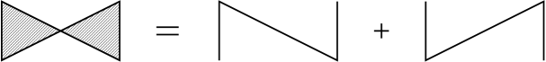
Figure 10: With successive emissions and absorptions vetoed, the two types of exchanges can be combined in a single rung.

5 Bethe-Salpeter with Veto

The Bethe-Salpeter equation for the discretized ’t Hooft model, with the veto imposed as described at the end of the previous section, is

$$\Psi(l) = \sum_{r=1}^{M-l-1}{\kappa^{2}\over r^{2}}u\alpha^{1/l+1/(M-l-r)}{\cal D}_{q\bar{q}}(l+r)\Psi(l+r)$$ (5.1)

$$\qquad\qquad+\sum_{r=1}^{l-1}{\kappa^{2}\over r^{2}}u\alpha^{1/(l-r)+1/(M-l)}{\cal D}_{q\bar{q}}(l-r)\Psi(l-r),$$

where ${\cal D}_{q\bar{q}}$ is defined in Eq. 4.8. After re-indexing both sums the equation can be written as

$$\Psi(l)=\sum_{r=l+1}^{M-1}{u\kappa^{2}\over(l-r)^{2}}\alpha^{1/l+1/(M-r)}{\cal D}_{q\bar{q}}(r)\Psi(r)+\sum_{r=1}^{l-1}{u\kappa^{2}\over(l-r)^{2}}\alpha^{1/r+1/(M-l)}{\cal D}_{q\bar{q}}(r)\Psi(r).$$ (5.2)

By imposing the veto we have reduced the rank of the eigenvalue problem from $2(M-2)$ to $M-1$.

The new discretized equation is much easier to analyze in the formal continuum limit $M\rightarrow\infty$ than the original. First define $\Phi(r)\equiv{\cal D}_{q\bar{q}}(r)\Psi(r)$, and rearrange Eq. 5.2 to read

$$K(l)\Phi(l) \equiv \left({1\over u{\cal D}_{q\bar{q}}(l)}-\kappa^{2}(\Sigma^{\prime}_{l}+\Sigma^{\prime}_{M-l})\right)\Phi(l)$$

$$= \sum_{r=l+1}^{M-1}{\kappa^{2}\over(l-r)^{2}}\alpha^{1/l+1/(M-r)}(\Phi(r)-\Phi(l))+\sum_{r=1}^{l-1}{\kappa^{2}\over(l-r)^{2}}\alpha^{1/r+1/(M-l)}(\Phi(r)-\Phi(l)).$$

To formally examine the continuum limit we suppose that each discrete $p^{+}$ variable is large putting each $l\rightarrow xM$, and take $M\rightarrow\infty$ at fixed $x$. Then the right hand side of Eq. 5 is set up to go to $1/M$ times the r.h.s. of the continuum ’t Hooft equation:

$$\hskip-56.9055pt\sum_{r=l+1}^{M-1}{\kappa^{2}\over(l-r)^{2}}\alpha^{1/l+1/(M-r)}(\Phi(r)-\Phi(l))+\sum_{r=1}^{l-1}{\kappa^{2}\over(l-r)^{2}}\alpha^{1/r+1/(M-l)}(\Phi(r)-\Phi(l))$$

$$\hskip 56.9055pt\rightarrow{\kappa^{2}\over M}P\int_{0}^{1}dy{\Phi(y)-\Phi(x)\over(y-x)^{2}}.$$ (5.4)

Clearly, $u$ must be chosen so that the l.h.s. is also of order $1/M$. Next, it is easy to verify that $\Sigma^{\prime}_{l}=\alpha^{1/l+1/(M-l)}(\pi^{2}/6-1/l+{\cal O}(\ln l/l^{2}))$, so that the inverse propagator can be simplified, neglecting terms of order $\ln M/M^{2}$,

$${1\over u_{l}{\cal D}_{q\bar{q}}(l)}\sim{1\over u_{l}^{2}}-\kappa^{4}\left({\pi^{2}\over 6}-{M\over 2l(M-l)}\right)^{2}-{1\over u_{l}}{1-u_{l}\kappa^{2}(\pi^{2}/6-M/2l(M-l))\over 1+u_{l}\kappa^{2}(\pi^{2}/6-M/2l(M-l))},$$ (5.5)

where we have defined $u_{l}=u\alpha^{M/l(M-l)}$. The factor $K$ multiplying $\Phi$ on the l.h.s. of Eq. 5 can now be simplified to

$$K(l) \sim \alpha^{M/l(M-l)}\left[{1\over u_{l}^{2}}-{\kappa^{4}\pi^{4}\over 36}-{1\over u_{l}}{1-u_{l}\kappa^{2}(\pi^{2}/6-M/2l(M-l))\over 1+u_{l}\kappa^{2}(\pi^{2}/6-M/2l(M-l))}-{\kappa^{2}\pi^{2}\over 3}\right.$$ (5.6)

$$\hskip 198.7425pt\mbox{}\left.+{\kappa^{4}\pi^{2}\over 6}{M\over l(M-l)}+\kappa^{2}{M\over l(M-l)}\right]$$

$$\sim \alpha^{M/l(M-l)}\left[{1\over u_{l}^{2}}-{\kappa^{4}\pi^{4}\over 36}-{1\over u_{l}}{1-u_{l}\kappa^{2}\pi^{2}/6\over 1+u_{l}\kappa^{2}\pi^{2}/6}-{\kappa^{2}\pi^{2}\over 3}\right.$$

$$\mbox{}\hskip 144.54pt\left.+{M\over l(M-l)}\left[{\kappa^{4}\pi^{2}\over 6}+\kappa^{2}-{\kappa^{2}\over(1+u_{l}\kappa^{2}\pi^{2}/6)^{2}}\right]\right]$$

Now write $u=u_{0}e^{a\Delta}$, where $a\Delta$ will be determined to be of order $1/M$, so that $u_{l}=u_{0}(1+a\Delta+(M/l(M-l))\ln\alpha)$ to order $1/M$. Then $u_{0}$ must satisfy

$$f(u_{0})\equiv{1\over u_{0}^{2}}-{\kappa^{4}\pi^{4}\over 36}-{1\over u_{0}}{1-u_{0}\kappa^{2}\pi^{2}/6\over 1+u_{0}\kappa^{2}\pi^{2}/6}-{\kappa^{2}\pi^{2}\over 3}=0.$$ (5.7)

Then the continuum limit reads

$$\left[a\Delta+{1\over Mx(1-x)}\left\{\ln\alpha+{1\over u_{0}f^{\prime}(u_{0})}\left[{\kappa^{4}\pi^{2}\over 6}+\kappa^{2}-{\kappa^{2}\over(1+u_{0}\kappa^{2}\pi^{2}/6)^{2}}\right]\right\}\right]\Phi(x)$$

$$\hskip-108.405pt=\quad{\kappa^{2}\over Mu_{0}f^{\prime}(u_{0})}P\int_{0}^{1}dy{\Phi(y)-\Phi(x)\over(y-x)^{2}}.\hskip 0.0pt$$

The energy of the system is $E=(\ln u_{0})/a+\Delta$, but the divergent first term is simply a physically irrelevant $M$ independent constant, so it is consistent to identify $P^{-}=\Delta$. Then ${\cal M}^{2}=2P^{+}P^{-}=2Mm\Delta=2MT_{0}a\Delta$. We also identify

$$\mu^{2}=-2T_{0}\left\{\ln\alpha+{1\over u_{0}f^{\prime}(u_{0})}\left[{\kappa^{4}\pi^{2}\over 6}+\kappa^{2}-{\kappa^{2}\over(1+u_{0}\kappa^{2}\pi^{2}/6)^{2}}\right]\right\},$$

and we obtain the continuum ’t Hooft equation

$$\left[{\cal M}^{2}-\mu^{2}{1\over x(1-x)}\right]\Phi(x) = {2T_{0}\kappa^{2}\over u_{0}f^{\prime}(u_{0})}P\int_{0}^{1}dy{\Phi(y)-\Phi(x)\over(y-x)^{2}}$$ (5.9)

$$= {g_{s}^{2}N_{c}\over 2\pi u_{0}f^{\prime}(u_{0})}P\int_{0}^{1}dy{\Phi(y)-\Phi(x)\over(y-x)^{2}}.$$

Comparing with Eq. 1.1, we see that the only effect on the continuum limit of keeping $T_{0}$ finite is a finite renormalization of the gauge coupling $g^{2}\rightarrow-g^{2}/u_{0}f^{\prime}(u_{0})$, and a coupling constant dependent shift in $\mu^{2}$. Thus, the only requirement for identical continuum physics is that $u_{0}f^{\prime}(u_{0})$ be negative. Since $\alpha$ is a free parameter, we can access all positive values of $\mu^{2}$ by tuning it.

Eq. 5.7 implicitly relates $u_{0}$ to $\kappa$ via a cubic equation. Instead of solving this equation, it is more illuminating to use it to relate $u_{0}$ to the combination $\eta\equiv u_{0}\kappa^{2}\pi^{2}/6$

$$u_{0}={(1-\eta^{2})(1+\eta)\over 1+\eta+2\eta^{2}},\qquad\kappa^{2}={6\eta\over u_{0}\pi^{2}}={6\eta(1+\eta+2\eta^{2})\over(1-\eta^{2})(1+\eta)\pi^{2}}.$$ (5.10)

We can also obtain the charge renormalization factor $u_{0}f^{\prime}(u_{0})$ in terms of $\eta$:

$$u_{0}f^{\prime}(u_{0})=-{(1+\eta+2\eta^{2})(1+\eta+7\eta^{2}-\eta^{3})\over(1-\eta^{2})^{2}(1+\eta)^{2}},$$ (5.11)

the effective coupling in the ’t Hooft equation

$${g_{\rm eff}^{2}N_{c}\over\pi}=-{2\kappa^{2}T_{0}\over u_{0}f^{\prime}(u_{0})}={12\eta(1-\eta^{2})(1+\eta)T_{0}\over\pi^{2}(1+\eta+7\eta^{2}-\eta^{3})},$$ (5.12)

and the renormalized mass parameter

$$\mu^{2}=\mu_{0}^{2}+{12\eta^{2}(3+\eta^{2})T_{0}\over\pi^{2}(1+\eta+7\eta^{2}-\eta^{3})},$$ (5.13)

where we have used $\alpha=e^{-\mu_{0}^{2}/2T_{0}}$.

As a check, note that the continuous time limit corresponds to $T_{0}\rightarrow\infty$ or $\kappa^{2}\rightarrow 0$, whence $u_{0}\rightarrow 1$ and $\eta\rightarrow 0$. Then the effective coupling Eq. 5.12 goes to $12T_{0}\eta/\pi^{2}=2T_{0}\kappa^{2}=g^{2}N_{c}/\pi=g_{s}^{2}N_{c}/2\pi$ as it should. Next, with discrete time, we see that, in order to have real energy and $\kappa$ ($u_{0}>0$ and $\kappa^{2}>0$), we must place the restriction $0<\eta<1$. Small $\kappa$ corresponds to small $\eta$, and large $\kappa$ corresponds to $\eta$ near unity. Interestingly, we note that the effective coupling in the ’t Hooft equation is small in both the small and large $\kappa$ regimes.

It is easy to understand the small effective coupling at large $\kappa$ in terms of our discrete time Feynman diagrams. With discrete time, $\kappa^{2}\rightarrow\infty$ causes the diagrams with a maximal number of powers of $\kappa^{2}$ per time step to dominate. For example the $q\bar{q}$ propagator ${\cal D}_{q\bar{q}}$ behaves in this limit as

$${\cal D}_{q\bar{q}}(l)\sim{u\alpha^{M/l(M-l)}\over 1-u^{2}\kappa^{4}\Sigma_{l}^{\prime}\Sigma_{M-l}^{\prime}}=u\alpha^{M/l(M-l)}\sum_{k=1}^{\infty}(u\kappa^{2})^{2k}(\Sigma_{l}^{\prime}\Sigma_{M-l}^{\prime})^{k},$$ (5.14)

so that the propagator for $2k+1$ time steps is $\alpha^{M/l(M-l)}(\kappa^{4}\Sigma_{l}^{\prime}\Sigma_{M-l}^{\prime})^{k}\rightarrow(\kappa^{2}\pi^{2}/6)^{2k}$ in the continuum limit. We see that away from the endpoints there is a factor of $\kappa^{2}\pi^{2}/6$ per time step in the continuum limit, which corresponds to each quark propagating exactly one time unit between interactions. Since this is the eigenvalue of the transfer matrix, we immediately infer the strong coupling value of $u_{0}=6/\kappa^{2}\pi^{2}$. Because of our veto, every exchange between quark lines occupies precisely two time steps and contributes only a single factor of $\kappa^{2}$. Thus each exchange costs a relative factor of $1/\kappa^{2}$ in the strong coupling limit, and this relative factor is proportional to the effective coupling in the ’t Hooft equation. More precisely, separating out the factor corresponding to the strong coupling propagation of the quark and anti-quark for two time steps, we have $\kappa^{2}=(\kappa^{2}\pi^{2}/6)^{2}(36/\kappa^{2}\pi^{4})$, so the effective coupling for a single exchange is $36/\kappa^{2}\pi^{4}$ for large $\kappa$, in accord with the $\eta\rightarrow 1$ limit of Eqs. 5.10, 5.12.

Now we turn to a numerical analysis of our discretized dynamics in order to understand how the continuum limit is approached in practice. As with the no-veto case in section 4 we can write this equation as an eigenvalue problem by rescaling $\Psi$ and isolating the eigenvalue $t$ as a function of $\chi\equiv u\kappa^{2}$. The resulting eigenvalue problem to solve is

$$t\Phi(l) = {\alpha_{l}\over\left(1-\chi^{2}\Sigma_{l}^{\prime}\Sigma_{M-l}^{\prime}\right)}\left[{\left(1-\chi\Sigma_{l}^{\prime}\right)\left(1-\chi\Sigma_{M-l}^{\prime}\right)\over\left(1-\chi^{2}\Sigma_{l}^{\prime}\Sigma_{M-l}^{\prime}\right)}\Phi(l)+\chi\sum_{r=1}^{l-1}{\alpha^{1/r+1/(M-l)}\over(l-r)^{2}}\Phi(r)\right.$$ (5.15)

$$\hskip 180.67499pt\left.+\chi\sum_{r=l+1}^{M-1}{\alpha^{1/l+1/(M-r)}\over(l-r)^{2}}\Phi(r)\right].$$

We use numerical procedures in MAPLE and MATLAB to find the eigenvalues $t_{n}(\chi)$ of the matrix on the right hand side of this equation as a function of $\chi$. The value of $\kappa^{2}$ is different for each $t_{n}$ since $\kappa^{2}=\chi t_{n}$. However by varying $0\leq\chi\leq\infty$ we can generate the real solutions, $t_{n}$, for all $\kappa^{2}$. In order to solve for complex $t_{n}$’s we would need to vary $\chi$ in the complex plane rather than just over positive real numbers.

  

  

Figure 11: Plots of the lowest lying energy eigenstates of the Bethe-Salpeter equation with the veto for $M=6,16,32,64$. Other states which occur at higher energies than those displayed have been omitted.

The problem of contamination of the lowest lying states by complex solutions has been solved by our veto prescription: The lowest lying state for $M=6$ for Eq. 5.15 remains intact for all coupling $\kappa^{2}$, see Fig. 11, which should be compared against Fig. 4 where the lowest lying state was only the ground state for $\kappa^{2}\lesssim 3$. When we analyze Eq. 5.15 for increasing $M$ (see Fig. 11 for $M=16,32,64$) we see that the number of low lying states that remain uncrossed for all couplings increases with increasing $M$. We also see that the spacing between these states decreases as $M$ increases. Recall that the solutions in Fig. 11 have been generated for $\alpha=0.5$.

In order to compare our numerical results for large values of $M$ (hopefully close to the continuum limit) with the numerical results of ’t Hooft [6] we solve the Bethe-Salpeter equation in Eq. 5.15 for $\kappa^{2}=0.5$ and

$$\alpha=1.16433\qquad\alpha=1.04167\qquad\alpha=0.70930.$$ (5.16)

These three choices of $\alpha$ correspond to values of ’t Hooft parameter, $\tilde{\mu}^{2}\equiv\pi\mu^{2}/g_{\rm eff}^{2}N_{c}$, taken to be $0$, $1$ and $2.11^{2}$ respectively. These values of $\tilde{\mu}$ were used in [6]. Fixing $\kappa^{2}$ is equivalent to fixing $\eta$, $u_{0}$ and $g_{\rm eff}^{2}N_{c}/\pi$, thus choosing a value for $\tilde{\mu}$ determines $\alpha$ in Eq. 5.13.

  

Figure 12: Plots of the three lowest lying states against $1/M$. The three graphs correspond to choices of $\alpha$ and $\kappa^{2}$ such that the continuum limit of $\tilde{\mu}^{2}\equiv\pi\mu^{2}/g_{\rm eff}^{2}N_{c}=0,1,(2.11)^{2}$ so that we can compare these results against those of ’t Hooft [6].

As we can see in Fig. 12 plots of the three lowest lying energy levels against $1/M$ show curves that become linear with increasing $M$. These results can be fitted to the functional form

$$aE=\ln(u_{0})+{c_{1}\over M}\exp\left({c_{2}\over M}+{c_{3}\over M^{2}}\right),$$ (5.17)

where $c_{2}$ and $c_{3}$ parameterize the departure from $1/M$ behaviour away from large $M$. We used the data of Fig. 12 in the range $128\leq M\leq 2048$ to fit this equation. With the fitted value of $c_{1}$ we can calculate the mass square of the corresponding bound state. As discussed previously, the $M$ independent term in Eq. 5.17 is dropped in identifying $P^{-}$. Since

$${\cal M}^{2}=2P^{+}P^{-}=2MT_{0}(aE-\ln{u_{0}}),$$ (5.18)

we have, for $\kappa^{2}=0.5$,

$${\cal M}^{2}={2c_{1}\over 0.22265}+\ldots,$$ (5.19)

in units of $g_{\rm eff}^{2}N_{c}/\pi$. The results of the fits are tabulated in Table 1 against the results of ’t Hooft [6].

	$\tilde{\mu}=0$	’t Hooft	$\tilde{\mu}=1$	’t Hooft	$\tilde{\mu}=2.11$	’t Hooft
ground state	0.72	0	7.25	7.2	24.23	24.1
1st	7.57	5.9	17.26	17.3	38.17	38.1
2nd	16.21	14.3	27.06	27.2	49.98	49.8

Table 1: Comparison of numerical fits for $128\leq M\leq 2048$ (for $\tilde{\mu}=0$ we used $128\leq M\leq 4096$) in order to determine the bound state mass squared in units of $g_{\rm eff}^{2}N_{c}/\pi$ for our discretized theory compared against the numerical results of the conventional continuous time approach of ’t Hooft.

We see that for $\tilde{\mu}=1$ and $2.11$, the results of our discretization match quite well those of [6]. However, for $\tilde{\mu}=0$ we increased the range of $M$ to 4096, which still yielded a poor match. What we did note was that even for these sizable values of $M$, convergence for $\tilde{\mu}=0$ is slow. When fitting the data for $\tilde{\mu}=0$ for the ground state to Eq. 5.17 we are trying to force it to fit a coefficient to a $1/M$ term which is not supposed to be there. It is more appropriate to use the form

$$aE=\ln(u_{0})+{c_{1}\over M^{\beta}}\exp\left({c_{2}\over M}+{c_{3}\over M^{2}}\right),$$ (5.20)

where the power $\beta$ of the leading behavior is fitted dynamically. We performed this refined fit to the three lowest lying states for $\tilde{\mu}=0$ which yielded the results assembled in Table 2.

	this$\beta$this
ground state	1.108
1st	1.025
2nd	1.015

Table 2: Table of fits to $\beta$ in Eq. 5.20 for $\tilde{\mu}=0$.

These results provide numerical evidence that for $\tilde{\mu}=0$, the 1st and 2nd excited states do have a nonzero meson mass (i.e. the leading behavior is $1/M$). However, the leading behavior for the ground state decreases more rapidly than $1/M$ and is consistent with zero meson mass.

We next address the issue of slow convergence for $\tilde{\mu}=0$ by examining the form of the ground energy eigenvector for increasing values of $M$. It is well known that the solutions of Eq. 1.1 for $\mu=0$ do not vanish at the endpoints $x=0,1$; indeed the exact ground state is simply a constant. As we can see in Fig. 13, at finite large $M$ the ground state solution of our discretized equation is ever smaller at the endpoints, and the progression of shapes is toward a more square profile. But even for $M=4096$ the eigenvector has not yet converged to its limiting form. This should be compared with the solution for $\tilde{\mu}=1$ which rapidly approaches it’s limiting form (see r.h.s. of Fig. 13). We see that, for our discretized equation, the solution for the ground state decreases more rapidly near the endpoints ($x=0$ and $x=1$) as $M$ increases, consistently with the shape eventually approaching a square profile at $M\rightarrow\infty$. However, it is not hard to show that consistency of the continuum limit requires that the range in $x$ over which the fall-off occurs must decrease less rapidly than $1/\sqrt{M}$. This still allows an approach to a square profile but convergence is necessarily slower than one might have expected. In fact all solutions of the continuum ’t Hooft equation with $\tilde{\mu}=0$ have non-zero values at the end points. Thus we should expect slow convergence for all solutions of the ${\tilde{\mu}}=0$ equation because the discrete solution tends to vanish at the endpoints but the limiting form does not. This effect does not occur for $\tilde{\mu}>0$ because then the continuum solution vanishes at the endpoints, so a decent approximation to it can be achieved with relatively smaller $M$.

  

Figure 13: Plot of the ground state eigenvector against $x=l/M$ for increasing $M$ for the cases $\tilde{\mu}=0$ and $1$. Each eigenvector is plotted for the range of $M$ indicated in powers of $2$.

6 Discussion and Conclusion

In this paper we have explored the efficacy of the discretization of large $N_{c}$ QCD proposed in [1] by applying it to the well-understood ’t Hooft model. For a smooth continuum limit over the whole range of bare coupling $\kappa$, we had to introduce a refinement of the discrete time gluon emission vertex. This amounted to insisting that after an emission, at least 2 time steps had to intervene before the next emission, with a similar restriction on consecutive absorptions. In contrast, an absorption is allowed to immediately follow an emission and vice versa. With this refinement in place we found that the continuum ’t Hooft equation describes the mass spectrum for all real $\kappa$. However, the parameters that occur in the equation are renormalized from their bare values, as summarized in Eqs. 5.10, 5.12, 5.13.

An amusing outcome of this renormalization phenomenon is that the effective coupling goes to zero in both the small and large $\kappa$ limits. Perhaps this feature is a version of weak/strong coupling duality, much celebrated in recent developments in string/M theory. However, we must concede that 2 dimensional QCD may be too trivial to expect anything other than the usual continuum theory to emerge from any continuum limit. Another caveat against attributing much significance to this “duality” phenomenon, is that the physics of the continuum limit really only depends on the ratio $\mu^{2}/N_{c}g^{2}$. This is because one can always choose the effective coupling as the fundamental unit of energy. Then the theories at different coupling but with the same value of this ratio (0 for example) are physically identical: any differences in description can be removed by a change of units.

At any rate, we conclude that the discretization of [1] can be meaningfully applied to QCD in 2 space-time dimensions, with some intriguing hints about the nature of weak/strong coupling duality. An obvious and important limitation of the 2 dimensional case, however, is that the gluon has no dynamical degrees of freedom. Thus there is no opportunity for the $P^{+}$ of the system to be shared amongst an infinite number of gluons. This must occur for the fishnet diagrams to be relevant, and is allowed in higher dimensional space-time. The next step is to study the three dimensional case, the simplest gauge theory where fishnet diagrams can be relevant.

Acknowledgements: We thank Klaus Bering for his helpful contributions in the early stages of this project.

References

[1]
K. Bering, J. S. Rozowsky and C. B. Thorn, Phys. Rev.D61 (2000)
045007, hep-th/9909141.
[2]
G. ’t Hooft, Nucl. Phys.B72 (1974) 461.
[3]
C. B. Thorn, Phys. Lett.70B (1977) 85; Phys. Rev.D17
(1978) 1073.
[4]
R. Giles, L. McLerran, and C. B. Thorn, Phys. Rev.D17 (1978) 2058.
[5]
R. Brower, R. Giles, and C. Thorn, Phys. Rev.D18 (1978) 484.
[6]
G. ’t Hooft, Nucl. Phys.B75 (1974) 461.
[7]
T. Maskawa and K. Yamawaki, Prog. Theor. Phys. 56 (1976) 270; A. Casher,
Phys. Rev. D14 (1976) 452.
[8]
S. J. Brodsky, H-C. Pauli, and S. J. Pinsky, Phys. Rept 301, (1998)
299; hep-ph/9705477.
[9]
E. E. Salpeter and H. A. Bethe, Phys. Rev.84 (1951) 1232.