Equation of state of cosmic strings with fermionic current-carriers

Abstract

The relevant characteristic features, including energy per unit length and tension, of a cosmic string carrying massless fermionic currents in the framework of the Witten model in the neutral limit are derived through quantization of the spinor fields along the string. The construction of a Fock space is performed by means of a separation between longitudinal modes and the so-called transverse zero energy solutions of the Dirac equation in the vortex. As a result, quantization leads to a set of naturally defined state parameters which are the number densities of particles and anti-particles trapped in the cosmic string. It is seen that the usual one-parameter formalism for describing the macroscopic dynamics of current-carrying vortices is not sufficient in the case of fermionic carriers.

I Introduction

The mechanism of spontaneous symmetry breaking involved in early universe phase transitions in some Grand Unified Theories (GUT) might lead to the formation of topological defects [1]. Among them, only cosmic strings happen to be compatible with observational cosmology if they form at the GUT scale. It was shown however by Witten [2] that, depending on the explicit realization of the symmetry breaking scheme as well as on the various particle couplings, a current could build along the strings, thereby effectively turning them into superconducting wires. Such wires were originally considered in the case the current couples to the electromagnetic field so they may be responsible for a variety of new effects, including an explosive scenario for large scale structure formation for which an enormous energy release was realized in the form of an expanding shell of non propagating photons in the surrounding plasma [3].

The cosmology of strings has been the subject of intense work in the last twenty years or so [4], mainly based on ordinary strings, global or local, aiming at deriving the large scale structure properties stemming from their distribution as well as their imprint in the microwave background [5]. It was even shown [6] that the most recent data [7] might support a non negligible contribution of such defects. As such a result requires ordinary strings, it turns out to be of uttermost importance to understand the influence of currents in the cosmological context.

Indeed, it can be argued that currents might drastically modify the cosmological evolution of a string network: The most clearly defined consequence of the existence of a current flowing along a vortex is the breaking of the boost invariance, since the current itself defines a privileged frame. In other words, the energy per unit length $U$ and the tension $T$ become two different numbers, contrary to the ordinary (Goto-Nambu [8]) case. As a result, string loops become endowed with the capability of rotation (the latter being meaningless for $U=T$), and the induced centrifugal force permits equilibrium configurations, called vortons [9]. They would very rapidly reach a regime where they would scale as ordinary non relativistic matter, until they come to completely dominate the Universe [10].

In the original Witten model [2], currents could form by means of two different mechanisms. Scalar fields, directly coupled with the string forming Higgs field, could feel a localized potential into which they could accumulate in the form of bound states, while fermions could be trapped along the string, propagating at the speed of light, as zero energy solutions of the two dimensional Dirac equation around the vortex. Other models were proposed where fermions could also propagate in the string core at lower velocities in the form of massive modes [11], or (possibly charged) vector fields could also condense [12]. All these models have essentially made clear that the existence of currents in string is much more than a mere possibility but rather an almost unavoidable fact in realistic particle physics theories.

For scalar as well as vector carriers, the task of understanding the microphysics is made simple thanks to their bosonic nature: all the trapped particles go into the same lowest accessible energy state and the field can be treated classically [13, 14]. Even the surrounding electromagnetic [15] and gravitational [16, 17] fields generated by the current can be treated this way and the backreaction can be included easily [18].

Meanwhile, a general formalism was set up by Carter [19] to describe current-carrying string dynamics. The formalism is based on a single so-called state parameter, $w$ say, of which the energy per unit length, the tension and the current itself are functions. Such a formalism relied heavily on the fact that for a bosonic carrier, the relevant quantity whose variation along the string leads to a current is its phase, and the state parameter is essentially identifiable to this phase gradient. Various equations of state relating the tension to the energy per unit length were then derived [20], based on numerical results and the existence of a phase frequency threshold [14]. It even includes the special case of a chiral current [21], although the latter originates in principle only for a purely fermionic current. Therefore, it was until now implicitly assumed that such a formalism would be sufficient to describe whatever current-carrying string configuration. It will be shown in this paper that this is in fact not true and an extended version, including more than one parameter, is needed [22].

The state parameter formalism, apart from being irrelevant for fermionic current-carrying strings, can only provide a purely classical description of their dynamics. This is unfortunate since the most relevant prediction of superconducting cosmic string models in cosmology is the existence of the vorton states discussed above. These equilibrium configurations of rotating loops are not necessarily stable, and in fact, this is perhaps the most important question to be answered on this topic. Indeed, any theory leading to the the existence of absolutely stable vortons predicts a cosmological catastrophe [10] and must be ruled out. One may therefore end up with a very stringent constraint on particle physics extension of the standard model of electroweak and strong interactions. To decide clearly on this point requires to investigate both the classical and the quantum stability of vortons.

Classical stability has already been established in the case of bosonic carriers [23] for whatever equation of state [24] on the basis of the one parameter formalism. Yet it will also have to be addressed in the more general context that will be discussed below. In the meantime it was believed that a quantum treatment was necessary in order to decide on the quantum stability: as one wants to compare the characteristic life-time of a vorton with the age of the Universe, quantum effects can turn out to be relevant; hence the following work in which the simplest of all fermionic Witten models is detailed [2] that can give rise to both spacelike as well as timelike charge currents, generalizing the usual point of view [25].

Let us sketch the lines along which this work is made.

A two-dimensional quantization of the spinor fields involved along a string is performed. Owing to anti-particle exitation states, one can derive the conditions under which the current is of arbitrary kind. Moreover, an equation of state giving the energy per unit length and the tension is obtained that involves four different state parameters which are found to be the number densities of fermions, although three of them only happen to be independent.

In section II, the model is presented and motivated, and the equations of motion are derived. Then in section III, we obtain plane wave solutions along the string by separating transverse and longitudinal dependencies of spinor fields in the vortex. The zero mode transverse solutions are then constraints to be normalizable in order to represent well defined wave functions. The quantization restricted to massless longitudinal modes is performed in section IV. As a result, the classical conserved currents obtained from Noether theorem, like energy-momentum tensor and fermionic currents, are expressed in their quantum form. All these quantum operators end up being functions of the fermionic occupation numbers only. In the last section (section V), the classical expressions for the energy per unit length and the tension are derived and discussed from computation of quantum observable values of the stress tensor operator in the classical limit. Contrary to the bosonic current-carrier case where there is only one state parameter [14], the classical limit of the model involves four state parameters in order to fully determine the energy per unit length and the tension. The cosmological consequences of this new analysis are briefly discussed in the concluding section.

II Equations of motion

We are going to be interested in the purely dynamical effects a fermionic current flowing along a cosmic string may have. The model we will be dealing with here is a simplified version of that proposed by Witten [2] which involves two kinds of fermions, in the neutral limit. This limit, for which the coupling between fermions and electromagnetic-like external fields is made to vanish, permits an easy recognition of the dynamical effects of the existence of an internal structure as in Ref. [14].

A Particle content

The model we shall consider involves a complex scalar Higgs field, $\Phi$ say, with conserved charge $qc_{\Phi}$ under a local $U(1)$ symmetry, together with the associated gauge vector field $B^{\mu}$. In this simple Abelian Higgs model [26], vortices can form after spontaneous breaking of the $U(1)$ symmetry. The minimal anomaly free model [2] with spinor fields requires two Dirac fermions denoted $\Psi$ and ${\mathcal{X}}$, with opposite electromagnetic-like charges, getting their masses from chiral coupling with the Higgs field and its complex conjugate. They also have conserved gauge charges from invariance under the broken $U(1)$ symmetry, $qc_{\psi_{R}}$, $qc_{\psi_{L}}$, $qc_{\chi_{R}}$, and $qc_{\chi_{L}}$, for the right- and left-handed parts of the two fermions respectively. The Lagrangian of the model therefore reads

$${\mathcal{L}}={\mathcal{L}}_{h}+{\mathcal{L}}_{g}+{\mathcal{L}}_{\psi}+{\mathcal{L}}_{\chi}$$ (1)

with ${\mathcal{L}}_{h}$, ${\mathcal{L}}_{g}$ and ${\mathcal{L}}_{\psi}$, ${\mathcal{L}}_{\chi}$, respectively the Lagrangian in the Higgs, gauge, and fermionic sectors. In terms of the underlying fields, they are

$${\mathcal{L}}_{h} = \frac{1}{2}(D_{\mu}\Phi)^{{\dagger}}(D^{\mu}\Phi)-V(\Phi),$$ (2)

$${\mathcal{L}}_{g} = -\frac{1}{4}H_{\mu\nu}H^{\mu\nu},$$ (3)

$${\mathcal{L}}_{\psi} = \frac{i}{2}\left[\overline{\Psi}\gamma^{\mu}D_{\mu}\Psi-(\overline{D_{\mu}\Psi})\gamma^{\mu}\Psi\right]-g\overline{\Psi}\frac{1+\gamma_{5}}{2}\Psi\Phi-g\overline{\Psi}\frac{1-\gamma_{5}}{2}\Psi\Phi^{\ast},$$ (4)

$${\mathcal{L}}_{\chi} = \frac{i}{2}\left[\overline{{{\mathcal{X}}}}\gamma^{\mu}D_{\mu}{{\mathcal{X}}}-(\overline{D_{\mu}{{\mathcal{X}}}})\gamma^{\mu}{{\mathcal{X}}}\right]-g\overline{{{\mathcal{X}}}}\frac{1+\gamma_{5}}{2}{{\mathcal{X}}}\Phi^{\ast}-g\overline{{{\mathcal{X}}}}\frac{1-\gamma_{5}}{2}{{\mathcal{X}}}\Phi,$$ (5)

where we have used the notation

$$D_{\mu}\Phi = (\nabla_{\mu}+iqc_{\phi}B_{\mu})\Phi,$$ (6)

$$D_{\mu}\Psi = (\nabla_{\mu}+iq\frac{c_{\psi_{R}}+c_{\psi_{L}}}{2}B_{\mu}+iq\frac{c_{\psi_{R}}-c_{\psi_{L}}}{2}\gamma_{5}B_{\mu})\Psi,$$ (7)

$$D_{\mu}{{\mathcal{X}}} = (\nabla_{\mu}+iq\frac{c_{\chi_{R}}+c_{\chi_{L}}}{2}B_{\mu}+iq\frac{c_{\chi_{R}}-c_{\chi_{L}}}{2}\gamma_{5}B_{\mu}){{\mathcal{X}}},$$ (8)

$$H_{\mu\nu} = \nabla_{\mu}B_{\nu}-\nabla_{\nu}B_{\mu},$$ (9)

$$V(\Phi) = \frac{\lambda}{8}(|\Phi|^{2}-\eta^{2})^{2}.$$ (10)

The equivalence with the Witten model [2] appears through a separation into left- and right-handed spinors. Let us define $\Psi_{R}$ and $\Psi_{L}$, respectively the right- and left-handed parts of the Dirac spinor field $\Psi$ (and the same for ${{\mathcal{X}}}$), eigenvectors of $\gamma_{5}$,

$$\Psi_{R}=\frac{1+\gamma_{5}}{2}\Psi, \Psi_{L}=\frac{1-\gamma_{5}}{2}\Psi.$$ and (11)

The Lagrangian for the spinor field $\Psi$ now reads

$${\mathcal{L}}_{\psi} = \frac{i}{2}\left[\overline{\Psi}_{R}\gamma^{\mu}D_{\mu}\Psi_{R}-(\overline{D_{\mu}\Psi}_{R})\gamma^{\mu}\Psi_{R}\right]+\frac{i}{2}\left[\overline{\Psi}_{L}\gamma^{\mu}D_{\mu}\Psi_{L}-(\overline{D_{\mu}\Psi}_{L})\gamma^{\mu}\Psi_{L}\right]-g\overline{\Psi}_{L}\Psi_{R}\Phi-g\overline{\Psi}_{R}\Psi_{L}\Phi^{\ast},$$ (12)

with the associated covariant derivatives

$$D_{\mu}\Psi_{R(L)}=(\nabla_{\mu}+iqc_{\psi_{R(L)}}B_{\mu})\Psi_{R(L)}.$$ (13)

It is clear with the Lagrangian expressed in this way that the invariance of the action under $U(1)$ transformations requires

$$c_{\psi_{L}}-c_{\psi_{R}}=c_{\phi}=c_{\chi_{R}}-c_{\chi_{L}}.$$ (14)

B Equations of motion

As we wish to deal with a cosmic string, the Higgs and gauge fields can be set as a vortex-like Nielsen–Olesen solution and they can be written in cylindrical coordinates as follows [30]

$$\begin{array}[]{ccc}\Phi=\varphi(r){\mathrm{e}}^{i\alpha(\theta)},&&B_{\mu}=B(r)\delta_{\mu\theta}.\end{array}$$ (15)

In order for the Higgs field to be well defined by rotation around the string, its phase has to be proportional to the orthoradial coordinate, $\alpha(\theta)=n\theta$, where the integer $n$ is the winding number. The new fields $\varphi$ and $\alpha$ are now real scalar fields and are solutions of the equations of motion

$$\nabla_{\mu}\nabla^{\mu}\varphi = \varphi Q_{\mu}Q^{\mu}-\frac{{\mathrm{d}}V(\varphi)}{{\mathrm{d}}\varphi}-\overline{\Psi}\frac{\partial m_{\psi}}{\partial\varphi}\Psi-\overline{{{\mathcal{X}}}}\frac{\partial m_{\chi}}{\partial\varphi}{{\mathcal{X}}},$$ (16)

$$\nabla_{\mu}\left(\varphi^{2}Q^{\mu}\right) = -\overline{\Psi}\frac{\partial m_{\psi}}{\partial\alpha}\Psi-\overline{{{\mathcal{X}}}}\frac{\partial m_{\chi}}{\partial\alpha}{{\mathcal{X}}},$$ (17)

where

$$Q_{\mu} = \nabla_{\mu}\alpha+qc_{\phi}B_{\mu},$$ (18)

$$m_{\psi} = g\varphi\cos{\alpha}+ig\varphi\gamma_{5}\sin{\alpha},$$ (19)

$$m_{\chi} = g\varphi\cos{\alpha}-ig\varphi\gamma_{5}\sin{\alpha}.$$ (20)

In the same way, the equations of motion for the gauge and spinor fields are

$$\nabla_{\mu}H^{\mu\nu} = j^{\nu}_{\psi}+j^{\nu}_{\chi}-qc_{\phi}\varphi^{2}Q^{\nu},$$ (21)

$$i\gamma^{\mu}\nabla_{\mu}\Psi = \frac{\partial j^{\mu}_{\psi}}{\partial\overline{\Psi}}B_{\mu}+m_{\psi}\Psi,$$ (22)

$$i\left(\nabla_{\mu}\overline{\Psi}\right)\gamma^{\mu} = -\frac{\partial j^{\mu}_{\psi}}{\partial\Psi}B_{\mu}-\overline{\Psi}m_{\psi},$$ (23)

$$i\gamma^{\mu}\nabla_{\mu}{{\mathcal{X}}} = \frac{\partial j^{\mu}_{\chi}}{\partial\overline{{{\mathcal{X}}}}}B_{\mu}+m_{\chi}{{\mathcal{X}}},$$ (24)

$$i\left(\nabla_{\mu}\overline{{{\mathcal{X}}}}\right)\gamma^{\mu} = -\frac{\partial j^{\mu}_{\chi}}{\partial{{\mathcal{X}}}}B_{\mu}-\overline{{{\mathcal{X}}}}m_{\chi}.$$ (25)

The fermionic currents $j^{\mu}_{\psi(\chi)}$ have axial and vectorial components due to the different coupling between left- and right-handed spinors to the gauge field. The two kinds of current are required to respect gauge invariance of the Lagrangian. In terms of spinor fields, they read

$$j^{\mu}_{\psi(\chi)}=j^{\mu}_{\psi_{V}(\chi_{V})}+j^{\mu}_{\psi_{A}(\chi_{A})},$$ (26)

with

$$\begin{array}[]{ccccccclll}j^{\mu}_{\psi_{V}}&=&q\displaystyle{\frac{c_{\psi_{R}}+c_{\psi_{L}}}{2}}\overline{\Psi}\gamma^{\mu}\Psi,&&j^{\mu}_{\chi_{V}}&=&q\displaystyle{\frac{c_{\chi_{R}}+c_{\chi_{L}}}{2}}\overline{{{\mathcal{X}}}}\gamma^{\mu}{{\mathcal{X}}},\\ \\ j^{\mu}_{\psi_{A}}&=&q\displaystyle{\frac{c_{\psi_{R}}-c_{\psi_{L}}}{2}}\overline{\Psi}\gamma^{\mu}\gamma_{5}\Psi,&&j^{\mu}_{\chi_{A}}&=&q\displaystyle{\frac{c_{\chi_{R}}-c_{\chi_{L}}}{2}}\overline{{{\mathcal{X}}}}\gamma^{\mu}\gamma_{5}{{\mathcal{X}}}.\end{array}$$ (27)

III Transverse solutions as Zero Modes

A Plane wave solutions

The study of the fermionic fields trapped along the string can be performed by separating the longitudinal and transverse solutions of the equations of motion. The plane wave solutions are therefore expressed in the generic form

$$\begin{array}[]{lll}\Psi_{p}^{(\pm)}={\mathrm{e}}^{\pm i(\omega t-kz)}\left(\begin{array}[]{l}\xi_{1}(r){\mathrm{e}}^{-im_{1}\theta}\\ \xi_{2}(r){\mathrm{e}}^{-im_{2}\theta}\\ \xi_{3}(r){\mathrm{e}}^{-im_{3}\theta}\\ \xi_{4}(r){\mathrm{e}}^{-im_{4}\theta}\end{array}\right),&&{{\mathcal{X}}}_{p}^{(\pm)}={\mathrm{e}}^{\pm i(\omega t-kz)}\left(\begin{array}[]{l}\zeta_{1}(r){\mathrm{e}}^{-il_{1}\theta}\\ \zeta_{2}(r){\mathrm{e}}^{-il_{2}\theta}\\ \zeta_{3}(r){\mathrm{e}}^{-il_{3}\theta}\\ \zeta_{4}(r){\mathrm{e}}^{-il_{4}\theta}\end{array}\right).\end{array}$$ (28)

Inside the vortex, the numbers $m_{i}$ and $l_{i}$ have to be integers in order to produce well defined spinors by rotation around the string. In the following, the Dirac spinors will be expressed in the chiral representation, and the metric is assumed to have the signature $(+,-,-,-)$. Plugging the expression (28) into the equations of motion (22) and (24) yields the differential system

$$\left\{\begin{array}[]{lll}\vspace{4pt}\displaystyle\left(\frac{{\mathrm{d}}\xi_{1}}{{\mathrm{d}}r}+\frac{1}{r}\left[-qc_{\psi_{R}}B(r)+m_{1}\right]\xi_{1}(r)\right){\mathrm{e}}^{-i(m_{1}-1)\theta}-ig\varphi(r){\mathrm{e}}^{-i(m_{4}+n)\theta}\xi_{4}(r)&=&\mp i(k+\omega)\xi_{2}(r){\mathrm{e}}^{-im_{2}\theta},\\ \vspace{4pt}\displaystyle\left(\frac{{\mathrm{d}}\xi_{2}}{{\mathrm{d}}r}+\frac{1}{r}\left[qc_{\psi_{R}}B(r)-m_{2}\right]\xi_{2}(r)\right){\mathrm{e}}^{-i(m_{2}+1)\theta}-ig\varphi(r){\mathrm{e}}^{-i(m_{3}+n)\theta}\xi_{3}(r)&=&\pm i(k-\omega)\xi_{1}(r){\mathrm{e}}^{-im_{1}\theta},\\ \vspace{4pt}\displaystyle\left(\frac{{\mathrm{d}}\xi_{3}}{{\mathrm{d}}r}+\frac{1}{r}\left[-qc_{\psi_{L}}B(r)+m_{3}\right]\xi_{3}(r)\right){\mathrm{e}}^{-i(m_{3}-1)\theta}+ig\varphi(r){\mathrm{e}}^{-i(m_{2}-n)\theta}\xi_{2}(r)&=&\mp i(k-\omega)\xi_{4}(r){\mathrm{e}}^{-im_{4}\theta},\\ \displaystyle\left(\frac{{\mathrm{d}}\xi_{4}}{{\mathrm{d}}r}+\frac{1}{r}\left[qc_{\psi_{L}}B(r)-m_{4}\right]\xi_{4}(r)\right){\mathrm{e}}^{-i(m_{4}+1)\theta}+ig\varphi(r){\mathrm{e}}^{-i(m_{1}-n)\theta}\xi_{1}(r)&=&\pm i(k+\omega)\xi_{3}(r){\mathrm{e}}^{-im_{3}\theta}.\end{array}\right.$$ (29)

Similar equations are obtained for the field ${{\mathcal{X}}}$ with the following transformations, $\xi\rightarrow\zeta$, $c_{\psi_{R(L)}}\rightarrow c_{\chi_{R(L)}}$, and $n\rightarrow-n$, because of its coupling to the anti-vortex instead of the vortex. Note that if, instead of the vectorial phases ansatz (28), we had chosen a matricial phases ansatz in the form

$$\Psi_{p}^{(\pm)}={\mathrm{e}}^{\pm i(\omega t-kz)}\left(\begin{array}[]{llll}\xi_{11}(r){\mathrm{e}}^{-im_{11}\theta}+\ldots+\xi_{14}(r){\mathrm{e}}^{-im_{14}\theta}\\ \xi_{21}(r){\mathrm{e}}^{-im_{21}\theta}+\ldots+\xi_{24}(r){\mathrm{e}}^{-im_{24}\theta}\\ \xi_{31}(r){\mathrm{e}}^{-im_{31}\theta}+\ldots+\xi_{34}(r){\mathrm{e}}^{-im_{34}\theta}\\ \xi_{41}(r){\mathrm{e}}^{-im_{41}\theta}+\ldots+\xi_{44}(r){\mathrm{e}}^{-im_{44}\theta}\end{array}\right),$$ (30)

we would have found, from the requirement of having at most four independent phases in the equations of motion, that the matrix $m_{ij}$ has to verify for all $i$, $m_{ij}=m_{ik}$, for all $(j,k)$. Consequently, the vectorial ansatz (28) is the most general for solutions with separated variables.

B Transverse solutions

From the differential system (29), it is obvious that the four phases $m_{i}$ cannot be independent parameters if the spinors fields are not identically zero. It is also impossible to find three independent phase parameters since each equation involves precisely three different angular dependencies. The only allowed angular separation requires two degrees of freedom in $\theta$, and the only relevant relation for trapped modes in the string reads from Eq. (29)

$$m_{1}-1=m_{4}+n, m_{2}+1=m_{3}+n.$$ (31)

1 Zero modes

Introducing the two integer parameters $p=m_{1}$ and $q=m_{3}$, and using equation (31), for $p\neq q+n$, the system (29) reduces to the set

$$\left\{\begin{array}[]{l}\vspace{4pt}\displaystyle\frac{{\mathrm{d}}\xi_{2}}{{\mathrm{d}}r}+\frac{1}{r}\left[qc_{\psi_{R}}B(r)-(q+n-1)\right]\xi_{2}(r)-ig\varphi(r)\xi_{3}(r)=0,\\ \vspace{4pt}\displaystyle\frac{{\mathrm{d}}\xi_{3}}{{\mathrm{d}}r}+\frac{1}{r}\left[-qc_{\psi_{L}}B(r)+q\right]\xi_{3}(r)+ig\varphi(r)\xi_{2}(r)=0,\\ \vspace{4pt}\displaystyle(k+\omega)\xi_{2}(r)=0,\\ \displaystyle(k+\omega)\xi_{3}(r)=0,\end{array}\right.$$ (32)

$$\left\{\begin{array}[]{l}\vspace{4pt}\displaystyle\frac{{\mathrm{d}}\xi_{1}}{{\mathrm{d}}r}+\frac{1}{r}\left[-qc_{\psi_{R}}B(r)+p\right]\xi_{1}(r)-ig\varphi(r)\xi_{4}(r)=0,\\ \vspace{4pt}\displaystyle\frac{{\mathrm{d}}\xi_{4}}{{\mathrm{d}}r}+\frac{1}{r}\left[qc_{\psi_{L}}B(r)-(p-n-1)\right]\xi_{4}(r)+ig\varphi(r)\xi_{1}(r)=0,\\ \vspace{4pt}\displaystyle(k-\omega)\xi_{1}(r)=0,\\ \displaystyle(k-\omega)\xi_{4}(r)=0.\end{array}\right.$$ (33)

There are two kinds of solutions which propagate along the two directions of the string at the speed of light and which were originally found by Witten [2]: Either $k=\omega$ and $\xi_{2}=\xi_{3}=0$, or $k=-\omega$ and $\xi_{1}=\xi_{4}=0$. These zero modes must also be normalizable in the transverse plane of the string in order to be acceptable as wave functions.

2 Index theorem

In the two cases $k=\omega$ and $k=-\omega$, we will call the corresponding zero modes, $X_{\psi}(r,\theta)$ and $Y_{\psi}(r,\theta)$, the solutions of the systems (32) and (33), respectively, i.e.,

$$\begin{array}[]{lll}X_{\psi}=\left(\begin{array}[]{l}0\\ \xi_{2}(r){\mathrm{e}}^{-i(q+n-1)\theta}\\ \xi_{3}(r){\mathrm{e}}^{-iq\theta}\\ 0\end{array}\right),&&Y_{\psi}=\left(\begin{array}[]{l}\xi_{1}(r){\mathrm{e}}^{-ip\theta}\\ 0\\ 0\\ \xi_{4}(r){\mathrm{e}}^{-i(p-n-1)\theta}\end{array}\right).\end{array}$$ (34)

These have to be normalizable in the sense that $\int{|X_{\psi}|^{2}r\,{\mathrm{d}}r\,{\mathrm{d}}\theta}$ and $\int{|Y_{\psi}|^{2}r\,{\mathrm{d}}r\,{\mathrm{d}}\theta}$ must be finite. Thanks to the regularity of the vortex background, the divergences in these integrals can only arise close to the string core or asymptotically far away from it. As a result, it is sufficient to study asymptotic behaviors of the solutions to decide on their normalizability [27].
Let us focus on the zero mode $X_{\psi}$ solution of Eq. (32), keeping in mind that $Y_{\psi}$ can be dealt with in the same way. The asymptotic behaviors at infinity are easily found as solutions of the limit at infinity of the differential system (32). Note that the identification between the equivalent solutions and the solutions of the equivalent system is only allowed by the absence of singular point for the system at infinity, and it will not be so near the string since $r=0$ is a singular point, so that the Cauchy theorem does no longer apply. From Eq. (32), the eigensolutions of the equivalent system at infinity are in the form $\exp{(\pm g\eta r)}$, and thus, there is only one normalizable solution at infinity.

Near the string, i.e., where $r\rightarrow 0$, the system is no longer well defined, the origin being a singular point. Approximate solutions can however be found by looking at the leading term of a power-law expansion of both system and functions, as originally suggested by Jackiw and Rossi [27]. Because the Cauchy theorem does no longer apply, many singular solutions might be found at the origin, and among them, the two generic ones which match with the two exponentials at infinity. Near the origin, the Higgs and gauge fields are known to behave like [30]

$$\begin{array}[]{lll}\varphi(r)\sim\varphi_{o}r^{|n|},&&B(r)\propto r^{2},\end{array}$$ (35)

so that the leading contribution near the string of the zero modes can be found as

$$\xi_{2}(r) \sim a_{2}r^{\alpha_{2}},$$ (36)

$$\xi_{3}(r) \sim a_{3}r^{\alpha_{3}},$$ (37)

with $a_{i}$ and $\alpha_{i}$ real parameters to be determined. The values of the exponents $\alpha_{i}$ are therefore given by the leading order terms in system (32), and one obtains three solutions, the first one of which being singular,

$$\begin{array}[]{lllll}\left(\begin{array}[]{l}\xi_{2}\\ \xi_{3}\end{array}\right)_{s}=\left(\begin{array}[]{l}a_{2}r^{q+n-1}\\ a_{3}r^{-q}\end{array}\right),&&\textrm{provided}&&\displaystyle-\frac{|n|+n}{2}<q<1+\frac{|n|-n}{2}.\end{array}$$ (38)

The two other solutions are the generic ones which have to match with the solutions at infinity

$$\begin{array}[]{lllllllll}\left(\begin{array}[]{l}\xi_{2}\\ \xi_{3}\end{array}\right)_{g1}&=&\left(\begin{array}[]{l}a_{2}(a_{3})r^{-q+|n|+1}\\ a_{3}r^{-q}\end{array}\right),&&\textrm{and}&&\left(\begin{array}[]{l}\xi_{2}\\ \xi_{3}\end{array}\right)_{g2}&=&\left(\begin{array}[]{l}a_{2}(a_{3})r^{q+n-1}\\ a_{3}r^{q+|n|+n}\end{array}\right),\end{array}$$ (39)

where the relationships between the parameters $a_{i}$ have not been written, since they are clearly obtained from Eq. (32). Normalizability near the origin requires that the integrals $\int{|\xi_{2}|^{2}\,r\,{\mathrm{d}}r}$ and $\int{|\xi_{3}|^{2}\,r\,{\mathrm{d}}r}$ converge, and this yields

$$-n<q<1.$$ (40)

Analogous considerations for the system (33) show the convergence criterion in this case to be

$$n<p<1.$$ (41)

The number of sets of parameters $p$ and $q$ satisfying the previous inequalities is precisely the number of well defined zero modes, respectively $Y_{\psi}$ and $X_{\psi}$, which are also normalizable. In order to match with the single well behaved solution at infinity, the two independent solutions near the string have to be integrable. Therefore, for a vortex solution with a positive winding number $n$, there are only $n$ normalizable zero modes, which are the $X_{\psi}$ ones. Similarly in the case of an anti-vortex with negative winding number $-|n|$, one finds also $|n|$ zero modes $Y_{\psi}$. This is the index theorem found by Jackiw and Rossi [27]. Recall that the model involves two kinds of fermions, and all the previous considerations apply as well for the field ${{\mathcal{X}}}$ with the simple transformation $n\rightarrow-n$. Therefore, the normalizable zero modes are swapped compared to those of the field $\Psi$.

Finally, for a vortex with positive winding number $n$, there are always $n$ massless plane wave solutions for both spinor fields, which read

$$\Psi_{p}^{(\pm)}={\mathrm{e}}^{\pm ik(t+z)}\left(\begin{array}[]{llll}0\\ \xi_{2}(r){\mathrm{e}}^{-i(q+n-1)\theta}\\ \xi_{3}(r){\mathrm{e}}^{-iq\theta}\\ 0\end{array}\right)={\mathrm{e}}^{\pm ik(t+z)}X_{\psi}(r,\theta),$$ (42)

$${{\mathcal{X}}}_{p}^{(\pm)}={\mathrm{e}}^{\pm ik(t-z)}\left(\begin{array}[]{llll}\zeta_{1}(r){\mathrm{e}}^{-ip\theta}\\ 0\\ 0\\ \zeta_{4}(r){\mathrm{e}}^{-i(p+n-1)\theta}\end{array}\right)={\mathrm{e}}^{\pm ik(t-z)}Y_{\chi}(r,\theta),$$ (43)

with now $q=m_{3}$ and $p=l_{1}$ which satisfy

$$\begin{array}[]{ccccc}-n<q<1,&&\textrm{and}&&-n<p<1.\end{array}$$ (44)

Note that they are eigenvectors of the $\gamma^{0}\gamma^{3}$ operator, and they basically verify

$$\begin{array}[]{llllllllllllllllll}\overline{X_{\psi}}\gamma^{0}X_{\psi}&=&|X_{\psi}|^{2},&&\overline{X_{\psi}}\gamma_{5}\gamma^{0}X_{\psi}&=&-|\xi_{2}|^{2}+|\xi_{3}|^{2},&&\overline{X_{\psi}}\gamma^{3}X_{\psi}&=&-|X_{\psi}|^{2},\\ \\ \overline{X_{\psi}}\gamma^{1(2)}X_{\psi}&=&0,&&\overline{X_{\psi}}\gamma_{5}\gamma^{3}X_{\psi}&=&|\xi_{2}|^{2}-|\xi_{3}|^{2},&&\overline{X_{\psi}}\gamma_{5}\gamma^{1(2)}X_{\psi}&=&0,\\ \\ \overline{Y_{\psi}}\gamma^{0}Y_{\psi}&=&|Y_{\psi}|^{2},&&\overline{Y_{\psi}}\gamma_{5}\gamma^{0}Y_{\psi}&=&-|\xi_{1}|^{2}+|\xi_{4}|^{2},&&\overline{Y_{\psi}}\gamma^{3}Y_{\psi}&=&|Y_{\psi}|^{2},\\ \\ \overline{Y_{\psi}}\gamma^{1(2)}Y_{\psi}&=&0,&&\overline{Y_{\psi}}\gamma_{5}\gamma^{3}Y_{\psi}&=&-|\xi_{1}|^{2}+|\xi_{4}|^{2},&&\overline{Y_{\psi}}\gamma_{5}\gamma^{1(2)}Y_{\psi}&=&0.\end{array}$$ (45)

The ${{\mathcal{X}}}$ zero modes $X_{\chi}$ and $Y_{\chi}$ verify the same relationships with $\xi_{i}$ replaced by $\zeta_{i}$.

3 Massive modes

The case $m_{1}=m_{3}+n$ allows four-dimensional solutions of the system (29). In Particular, these solutions do no longer require $\omega=\pm k$ and therefore represent massive modes. As before, the interesting behaviors of these modes are found by studying the solutions of the equivalent system asymptotically and by looking for the leading term of a power-law expansion of both system and solution near the string core.

At infinity, the system is well defined and there are two twice degenerate eigensolutions $\exp{(\pm\Omega r)}$ out of which two are normalizable, with

$$\Omega=\sqrt{g^{2}\eta^{2}-(\omega^{2}-k^{2})}.$$ (46)

Near the origin, at $r=0$, the system is singular, and because of its four dimensions there are much more singular solutions than the previous two dimensional case, and among them the four generic ones which match with the four ones at infinity. The leading term in asymptotic expansion can be written in a standard way

$$\xi_{i}(r)\sim a_{i}r^{\alpha_{i}}.$$ (47)

Plugging these expressions in the system (29) with Eq. (35), and keeping only leading terms at $r=0$ gives, after some algebra, the four generic solutions

$$\begin{array}[]{lllllll}\left(\begin{array}[]{l}\xi_{1}\\ \xi_{2}\\ \xi_{3}\\ \xi_{4}\end{array}\right)_{g1}&=&\left(\begin{array}[]{l}a_{1}r^{-m}\\ a_{2}(a_{1})r^{-m+1}\\ a_{3}(a_{1})r^{-m+|n|+2}\\ a_{4}(a_{1})r^{-m+|n|+1}\end{array}\right),&&\left(\begin{array}[]{l}\xi_{1}\\ \xi_{2}\\ \xi_{3}\\ \xi_{4}\end{array}\right)_{g2}&=&\left(\begin{array}[]{l}a_{1}r^{m+|n|-n}\\ a_{2}(a_{1})r^{m+|n|-n+1}\\ a_{3}(a_{1})r^{m-n}\\ a_{4}(a_{1})r^{m-n-1}\end{array}\right),\\ \\ \left(\begin{array}[]{l}\xi_{1}\\ \xi_{2}\\ \xi_{3}\\ \xi_{4}\end{array}\right)_{g3}&=&\left(\begin{array}[]{l}a_{1}r^{m}\\ a_{2}(a_{1})r^{m-1}\\ a_{3}(a_{1})r^{m+|n|}\\ a_{4}(a_{1})r^{m+|n|+1}\end{array}\right),&&\left(\begin{array}[]{l}\xi_{1}\\ \xi_{2}\\ \xi_{3}\\ \xi_{4}\end{array}\right)_{g4}&=&\left(\begin{array}[]{l}a_{1}r^{-m+|n|+n+2}\\ a_{2}(a_{1})r^{-m+|n|+n+1}\\ a_{3}(a_{1})r^{-m+n}\\ a_{4}(a_{1})r^{-m+n+1}\end{array}\right),\end{array}$$ (48)

with $m=m_{1}$, and where the relationships between the coefficients $a_{i}$ have not been written as they are essentially given by a linear system in $a_{i}$ given by Eq. (29). The solutions (48) will be normalizable near the string if, for all $i$, $\int{|\xi_{i}|^{2}\,r\,{\mathrm{d}}r}$ is finite. Moreover there will be, at least, always one massive bound state if there are at least three normalizable eigensolutions to match with the well-defined ones at infinity. This is only allowed if the parameter $m$ verifies simultaneously three of the following conditions

$$\sup{(0,n)}<m<\inf{(1,1+n)}.$$ (49)

Because $m$ is necessary an integer, this condition cannot be achieved. This criterion, originally derived and used by Jackiw and Rossi in order to enumerate the number of zero modes in a vortex-fermion system [27], is only sufficient and thus, normalizable massive bound states may exist, but are model dependent since it is necessary that a particular combination of the two normalizable eigenmodes near the string core match exactly with a particular combination of the two well-defined ones at infinity.

Such massive bound states depend therefore of the particular values of the model parameters. Recently, it was shown numerically [25] that the Abelian Higgs model with one Weyl fermion admits always at least two massive bound states, as a result, the present toy model also may have such states. However, in order to simplify the quantization, we will only consider the generic zero modes, and consequently, the following results will be relevant for cosmic string only when the occupancy of the massive bound states can be neglected compared to the occupancy of the zero mode states. Such physical situations are likely to occur far below the energy scale where the string was formed, since the massive states are generally expected to decay much more rapidly than the massless ones [25].

The generic massless normalizable transverse solutions of the fermionic equations of motion in the string with winding number $n$ are the $n$ zero modes. For the spinor field $\Psi$ coupled with the vortex, we find that the particles and the anti-particles can only propagate at the speed of light in one direction, “$-z$” say direction along the string, whereas the spinor field ${{\mathcal{X}}}$ propagates in the opposite, “$+z$” direction. The existence of such plane waves allows us to quantize the spinor fields along the string. The zero modes themselves will therefore be transverse wave functions giving the probability density for finding a trapped mode at a chosen distance from the string core.

IV Fock space along the string

The spinor fields can be expanded on the basis of the plane wave solutions computed above. A canonical quantization can then be performed along the $z$-axis which provides analytical expressions for these fields in two dimensions once the transverse degrees of freedom have been integrated over. It is therefore possible to compute the current operators as well as their observable values given by their averages in a particular Fock state. In the following we shall take a vortex with a unit winding number $n=1$ and the subscript of the zero modes $X_{\psi}$ and $Y_{\chi}$ will be forgotten since there is not possible confusion.

A Canonical quantization

We shall first be looking for a physical expansion of the spinor fields in plane waves, in the sense that creation and annihilation operators are well defined. The Hamiltonian is then calculable as a function of these and will be required to be positive to yield a reasonable theory.

1 Quantum fields

As shown above, the spinor fields $\Psi$ and ${{\mathcal{X}}}$ propagate in only one direction, therefore in expressions (42) and (43) the momentum $k$ can be chosen positive definite. Let us, once again, focus on the spinor field $\Psi$. The natural way to expand it in plane waves of positive and negative energies is

$$\Psi=\int_{0}^{\infty}{\frac{{\mathrm{d}}k}{2\pi 2k}\left[b^{{\dagger}}(-k){\mathrm{e}}^{ik(t+z)}+\underline{b}(-k){\mathrm{e}}^{-ik(t+z)}\right]X}.$$ (50)

The Fourier transform of $\Psi$ on positive and negative energies has been written with similar notation $b^{\dagger}$ and $\underline{b}$ unlike in the free spinor case. Indeed, note that, in the string, the zero modes are the same for both positive and negative energy waves, so that the only way to distinguish particles from anti-particles is in the sign of the energy. The integration measure ${\mathrm{d}}k/(2\pi 2k)$ is the usual Lorentz invariant measure in two dimensions. Note that $k$ is chosen always positive in order to represent physical energy and momentum actually carried by the field along the string; hence the negative sign in $b^{\dagger}(-k)$ and $\underline{b}(-k)$, which is a reminder that the spinor field $\Psi$ propagates in the “$-z$” direction. In the same way, the field ${{\mathcal{X}}}$ is expanded as

$${{\mathcal{X}}}=\int_{0}^{\infty}{\frac{{\mathrm{d}}k}{2\pi 2k}\left[d^{{\dagger}}(k){\mathrm{e}}^{ik(t-z)}+\underline{d}(k){\mathrm{e}}^{-ik(t-z)}\right]Y}.$$ (51)

The Fourier transform will be written with the normalization convention

$$\int{{\mathrm{d}}z\,{\mathrm{e}}^{i(k-k^{\prime})z}}=2\pi\delta(k-k^{\prime}).$$ (52)

2 Creation and annihilation operators

The Fourier coefficients can be expressed as functions of the spinor field $\Psi$ or $\Psi^{\dagger}$. With equation (50) and (52), let us compute the following integral

$$\int{r\,{\mathrm{d}}r\,{\mathrm{d}}\theta\,{\mathrm{d}}z\,{\mathrm{e}}^{ik(t+z)}X^{\dagger}\Psi}=\int{\frac{{\mathrm{d}}k^{\prime}}{2k^{\prime}}\left[b^{\dagger}(-k^{\prime})\delta(k+k^{\prime})+b(-k^{\prime})\delta(k-k^{\prime})\right]}\|X\|^{2}=\frac{\|X\|^{2}}{2k}b(-k),$$ (53)

where we have defined

$$\|X\|^{2}\equiv\int{r\,{\mathrm{d}}r\,{\mathrm{d}}\theta\,|X|^{2}}.$$ (54)

Note that the separation between $b$ and $b^{\dagger}$ only arises from the chirality of the spinor field because the integration is performed only over positive values of the momentum $k$; this is why the $\delta(k+k^{\prime})$ term vanishes. In the following we will assume that the zero modes are normalized to unity, $\|X\|^{2}=1$, and $\|Y\|^{2}=1$. Playing with similar integrals gives us the other expansion coefficients

$$\begin{array}[]{ccccccclll}\underline{b}(-k)&=&2k\displaystyle\int{r\,{\mathrm{d}}r\,{\mathrm{d}}\theta\,{\mathrm{d}}z\,{\mathrm{e}}^{ik(t+z)}X^{\dagger}\Psi},&&\underline{b}^{\dagger}(-k)&=&2k\displaystyle\int{r\,{\mathrm{d}}r\,{\mathrm{d}}\theta\,{\mathrm{d}}z\,{\mathrm{e}}^{-ik(t+z)}\Psi^{\dagger}X},\\ \\ b^{\dagger}(-k)&=&2k\displaystyle\int{r\,{\mathrm{d}}r\,{\mathrm{d}}\theta\,{\mathrm{d}}z\,{\mathrm{e}}^{-ik(t+z)}X^{\dagger}\Psi},&&b(-k)&=&2k\displaystyle\int{r\,{\mathrm{d}}r\,{\mathrm{d}}\theta\,{\mathrm{d}}z\,{\mathrm{e}}^{ik(t+z)}\Psi^{\dagger}X},\end{array}$$ (55)

and the corresponding relations for the spinor field ${{\mathcal{X}}}$

$$\begin{array}[]{ccccccclll}d^{\dagger}(k)&=&2k\displaystyle\int{r\,{\mathrm{d}}r\,{\mathrm{d}}\theta\,{\mathrm{d}}z\,{\mathrm{e}}^{-ik(t-z)}Y^{\dagger}{{\mathcal{X}}}},&&d(k)&=&2k\displaystyle\int{r\,{\mathrm{d}}r\,{\mathrm{d}}\theta\,{\mathrm{d}}z\,{\mathrm{e}}^{ik(t-z)}{{\mathcal{X}}}^{\dagger}Y},\\ \\ \underline{d}(k)&=&2k\displaystyle\int{r\,{\mathrm{d}}r\,{\mathrm{d}}\theta\,{\mathrm{d}}z\,{\mathrm{e}}^{ik(t-z)}Y^{\dagger}{{\mathcal{X}}}},&&\underline{d}^{\dagger}(k)&=&2k\displaystyle\int{r\,{\mathrm{d}}r\,{\mathrm{d}}\theta\,{\mathrm{d}}z\,{\mathrm{e}}^{-ik(t-z)}{{\mathcal{X}}}^{\dagger}Y}.\end{array}$$ (56)

From these, one gets the necessary relations to define creation and annihilation operators

$$\begin{array}[]{ccccclll}\underline{b}^{\dagger}(-k)=\left[\underline{b}(-k)\right]^{\dagger},&&\textrm{and}&&b^{\dagger}(-k)=\left[b(-k)\right]^{\dagger},\\ \\ d^{\dagger}(k)=\left[d(k)\right]^{\dagger},&&\textrm{and}&&\underline{d}^{\dagger}(k)=\left[\underline{d}(k)\right]^{\dagger}.\end{array}$$ (57)

3 Commutation relations

The canonical quantization is performed by the transformation of Poisson brackets into anticommutators. Here, we want to quantize the spinor fields only along the string, and therefore let us postulate the anticommutation rules at equal times for the quantum fields

$$\left\{\Psi_{\alpha}(t,\vec{x}),\Psi^{{\dagger}\beta}(t,\vec{x}^{\prime})\right\} = \delta(z-z^{\prime})X_{\alpha}(r,\theta)X^{{\dagger}\beta}(r^{\prime},\theta^{\prime}),$$ (58)

$$\left\{{{\mathcal{X}}}_{\alpha}(t,\vec{x}),{{\mathcal{X}}}^{{\dagger}\beta}(t,\vec{x}^{\prime})\right\} = \delta(z-z^{\prime})Y_{\alpha}(r,\theta)Y^{{\dagger}\beta}(r^{\prime},\theta^{\prime}),$$ (59)

with $\alpha$ and $\beta$ the spinorial indices, and all the other anticommutators vanishing. With equation (55) and these anticommutation rules, it follows immediately, for creation and annihilation operators, that

$$\begin{array}[]{ccccclll}\left\{b(-k),b^{\dagger}(-k^{\prime})\right\}&=&\left\{\underline{b}(-k),\underline{b}^{\dagger}(-k^{\prime})\right\}&=&2\pi 2k2k^{\prime}\delta(k-k^{\prime}),\\ \\ \left\{\underline{d}(k),\underline{d}^{\dagger}(k^{\prime})\right\}&=&\left\{d(k),d^{\dagger}(k^{\prime})\right\}&=&2\pi 2k2k^{\prime}\delta(k-k^{\prime}),\end{array}$$ (60)

with all other anticommutators vanishing. From the expressions (50) and (51) and with the anticommutation rules (60), it is possible to derive the anticommutator between two quantum field operators at any time. For instance, the anticommutator between $\Psi$ and $\Psi^{\dagger}$ reads

$$\left\{\Psi_{\alpha}({\mathbb{x}}),\Psi^{{\dagger}\beta}({\mathbb{x}}^{\prime})\right\} = \int{\frac{{\mathrm{d}}k\,{\mathrm{d}}k^{\prime}}{(2\pi)^{2}2k2k^{\prime}}\left\{b^{\dagger}(-k){\mathrm{e}}^{ik(t+z)}+\underline{b}(-k){\mathrm{e}}^{-ik(t+z)},b(-k^{\prime}){\mathrm{e}}^{-ik^{\prime}(t^{\prime}+z^{\prime})}\right.}+$$ (61)

$$+ \left.\underline{b}^{\dagger}(-k^{\prime}){\mathrm{e}}^{ik^{\prime}(t^{\prime}+z^{\prime})}\right\}X_{\alpha}(r,\theta)X^{{\dagger}\beta}(r^{\prime},\theta^{\prime}).$$ (62)

Thanks to the delta function coming from the anticommutators between the $b$ and $b^{\dagger}$, this expression reduces to

$$\left\{\Psi_{\alpha}({\mathbb{x}}),\Psi^{{\dagger}\beta}({\mathbb{x}}^{\prime})\right\} = i\partial_{t}\Delta(t-t^{\prime}+z-z^{\prime})X_{\alpha}(r,\theta)X^{{\dagger}\beta}(r^{\prime},\theta^{\prime}),$$ (63)

with $\Delta({\mathbb{x}})$ the well known Pauli-Jordan function which vanishes for spacelike separation, so the spinor fields indeed respect micro-causality along the string.

4 Fock states

The Fock space can be built by application of the creation operators on the vacuum state $|\emptyset\rangle$ which by definition has to satisfy

$$\underline{b}(-k)|\emptyset\rangle=b(-k)|\emptyset\rangle=d(k)|\emptyset\rangle=\underline{d}(k)|\emptyset\rangle=0,$$ (64)

and is normalized to unity, i.e., $\langle\emptyset|\emptyset\rangle=1$. Each Fock state represents one possible combination of the fields exitation levels. Let $|{\mathcal{P}}\rangle$ be a Fock state representing $N_{\psi}$ particles labeled by $i$ and $\overline{N}_{\psi}$ anti-particles labeled by $j$, of kind $\Psi$, with respective momenta $k_{i}$ and $l_{j}$, and, $N_{\chi}$ particles labeled by $p$ and $\overline{N}_{\chi}$ anti-particles labeled by $q$, of kind ${{\mathcal{X}}}$, with respective momenta $r_{p}$ and $s_{q}$. By construction the state is

$$|{\mathcal{P}}\rangle = b^{\dagger}(-k_{1})\ldots b^{\dagger}(-k_{i})\ldots b^{\dagger}(-k_{N_{\psi}})\underline{b}^{\dagger}(-l_{1})\ldots\underline{b}^{\dagger}(-l_{j})\ldots\underline{b}^{\dagger}(-l_{\overline{N}_{\psi}})d^{\dagger}(r_{1})\ldots$$ (65)

$$\ldots d^{\dagger}(r_{p})\ldots d^{\dagger}(r_{N_{\chi}})\underline{d}^{\dagger}(s_{1})\ldots\underline{d}^{\dagger}(s_{q})\ldots\underline{d}^{\dagger}(s_{\overline{N}_{\chi}})|\emptyset\rangle.$$ (66)

Normalizing such a state is done thanks to the anticommutators (60). For instance, for a one particle $\Psi$ state with $k$ momentum, using Eq. (64), the orthonormalization of the corresponding states reads

$$\langle k^{\prime}|k\rangle=2\pi 2k2k^{\prime}\delta(k-k^{\prime}).$$ (67)

Obviously similar relations apply to all the other particle and anti-particle states. Keeping in mind that the observable values of quantum operators are their eigenvalues in a given quantum state, let us compute the average of the occupation number operator involved in many quantum operators, as will be shown. For $\Psi$ particles it is

$$\frac{\langle{\mathcal{P}}|b^{\dagger}(-k)b(-k^{\prime})|{\mathcal{P}}\rangle}{\langle{\mathcal{P}}|{\mathcal{P}}\rangle}=\frac{2\pi}{\delta(0)}2k2k^{\prime}\sum_{i}\delta(k-k_{i})\delta(k^{\prime}-k_{i})$$ (68)

and analogous relations for the other particle and anti-particle states. By definition of the Fourier transform (52), the infinite factor $\delta(0)$ is simply an artifact related to the length of the string $L$ by

$$L=2\pi\delta(0),$$ (69)

in the limit where this string length $L\to\infty$. Note that using periodic boundary conditions on $L$ allows to consider large loops with negligible radius of curvature.

B Fermionic energy momentum tensor

The simplest way to derive an energy momentum tensor already symmetrized is basically from the variation of the action with respect to the metric. Moreover, the Hamiltonian density of the fermion $\Psi$,

$${\mathcal{H}}_{\psi}=\partial_{t}\Pi_{\psi}\Psi+\partial_{t}\overline{\Psi}\overline{\Pi}_{\psi}-{\mathcal{L}}_{\psi},$$ (70)

with $\Pi$ the conjugate field $\Pi=i\overline{\Psi}\gamma^{0}$, is also equal to the $T_{\psi}^{tt}$ component of the stress tensor. In our case the metric is cylindrical and we assume a flat Minkowski space-time background, thus in the fermionic sector the stress tensor reads

$$T_{\psi}^{\mu\nu}=2\frac{\delta{\mathcal{L}}_{\psi}}{\delta g_{\mu\nu}}-g^{\mu\nu}{\mathcal{L}}_{\psi}\quad \quad T_{\chi}^{\mu\nu}=2\frac{\delta{\mathcal{L}}_{\chi}}{\delta g_{\mu\nu}}-g^{\mu\nu}{\mathcal{L}}_{\chi}.$$ and (71)

Once again, let us focus on $\Psi$. Plugging Eq. (4) into Eq. (71) gives

$$T_{\psi}^{\mu\nu}=\frac{i}{2}\overline{\Psi}\gamma^{(\mu}\partial^{\nu)}\Psi-\frac{i}{2}\left(\partial^{(\mu}\overline{\Psi}\right)\gamma^{\nu)}\Psi-B^{(\mu}j^{\nu)}_{{}_{\psi}}.$$ (72)

1 Symmetrized Hamiltonian

From Noether theorem, the Hamiltonian $P^{t}$ is also given by the conserved charge associated with the time component of the energy momentum tensor

$$T^{tt}_{\psi}=i\overline{\Psi}\gamma^{0}\partial_{t}\Psi-i\left(\partial_{t}\overline{\Psi}\right)\gamma^{0}\Psi.$$ (73)

Thanks to the expression of the quantum fields in equations (50) and (51), and using the properties of the zero modes from Eq. (45), the quantum operator associated to $T_{\psi}^{tt}$ reads

$$T_{\psi}^{tt} = \frac{1}{2}\int{\frac{{\mathrm{d}}k\,{\mathrm{d}}k^{\prime}}{(2\pi)^{2}2k}}\left[\left(-b(-k)b^{\dagger}(-k^{\prime})+\underline{b}^{\dagger}(-k^{\prime})\underline{b}(-k)\right){\mathrm{e}}^{i(k^{\prime}-k)(t+z)}\right.$$ (74)

$$+ \left.\left(\underline{b}^{\dagger}(-k)\underline{b}(-k^{\prime})-b(-k^{\prime})b^{\dagger}(-k)\right){\mathrm{e}}^{-i(k^{\prime}-k)(t+z)}\right.$$ (75)

$$+ \left.\left(b(-k)\underline{b}(-k^{\prime})-b(-k^{\prime})\underline{b}(-k)\right){\mathrm{e}}^{-i(k^{\prime}+k)(t+z)}\right.$$ (76)

$$+ \left.\left(-\underline{b}^{\dagger}(-k)b^{\dagger}(-k^{\prime})+\underline{b}^{\dagger}(-k^{\prime})b^{\dagger}(-k)\right){\mathrm{e}}^{i(k^{\prime}+k)(t+z)}\right]|X|^{2}.$$ (77)

The Hamiltonian is given by spatial integration of the Hamiltonian density, or similarly from Eq. (74),

$$P^{t}_{\psi}=\int{\frac{{\mathrm{d}}k}{2\pi 2k}\left[-b(-k)b^{\dagger}(-k)+\underline{b}^{\dagger}(-k)\underline{b}(-k)\right]}.$$ (78)

Note, once again, that all the terms in the form $b^{\dagger}b^{\dagger}$ or $b{}b$ vanish as a consequence of the chiral nature of the spinor fields which only allows $k>0$. The average value of this Hamiltonian in the vacuum is not at all positive, but a simple renormalization shift is sufficient to produce a reasonable Hamiltonian provided one uses fermionic creation and annihilation operators with the corresponding definition for the normal ordered product (antisymmetric form). The normal ordered Hamiltonian is therefore well behaved and reads

$$:P^{t}_{\psi}: = \int{\frac{{\mathrm{d}}k}{2\pi 2k}\left[b^{\dagger}(-k)b(-k)+\underline{b}^{\dagger}(-k)\underline{b}(-k)\right]}.$$ (79)

However, note that such a normal ordering prescription overlooks the differences between the vacuum energy of empty space, and that in the presence of the string for the massless fermions. Formally, from Eq. (74), the normal ordered Hamiltonian is also obtained by adding the operator $\int{{\mathrm{d}}\vec{x}\,{\mathrm{V}}_{\psi}}$ to the infinite Hamiltonian in Eq. (78), with

$${\mathrm{V}}_{\psi}=:T^{tt}_{\psi}:\,-\,T^{tt}_{\psi} = \frac{1}{2}\int{\frac{{\mathrm{d}}k\,{\mathrm{d}}k^{\prime}}{(2\pi)^{2}2k}}\left[\left\{b(-k),b^{\dagger}(-k^{\prime})\right\}{\mathrm{e}}^{i(k^{\prime}-k)(t+z)}\right.$$ (80)

$$+ \left.\left\{b(-k^{\prime}),b^{\dagger}(-k)\right\}{\mathrm{e}}^{-i(k^{\prime}-k)(t+z)}\right]|X|^{2}.$$ (81)

Owing to the anticommutation rules in Eq. (58), this expression reduces to

$${\mathrm{V}}_{\psi}=\int{\frac{{\mathrm{d}}k}{\pi}\,k\,|X|^{2}}.$$ (82)

This infinite renormalizing term of the vacuum associated with the zero modes on the string comes from the contribution of the infinite renormalization of the usual empty space together with a finite term representing the difference between the two kinds of vacua. The previous expression (82) emphasizes the structure of the divergence, and it can be conjectured that the finite part is simply obtained by a cut-off $\Lambda$ in momentum values. The finite vacuum contribution to the stress tensor can therefore be represented from Eq. (82), up to the sign, by the energy density

$$\frac{\Lambda^{2}}{2\pi}|X|^{2}=\frac{2\pi}{L_{v}^{2}}|X|^{2}, L_{v}=\frac{2\pi}{\Lambda}.$$ with (83)

The precise determination of the value of $L_{v}$ is outside the scope of this simple model. It is well known however, that the vacuum effects generally involve energies smaller than the first quantum energy level and consequently it seems reasonable to consider that $L_{v}>L$. For a large loop, $L_{v}$ can be roughly estimated using the discretization of the momentum values. With $k_{n}=2\pi n/L$, ${\mathrm{V}}_{\psi}$ therefore reads

$${\mathrm{V}}_{\psi}=\frac{4\pi}{L^{2}}|X|^{2}\sum_{n=0}^{\infty}n.$$ (84)

Assuming that the vacuum associated with the fermionic zero modes on the string matches the Minkowski one associated with massless fermionic modes, in the infinite string limit [31, 32], $L_{v}$ can be obtained by substracting the two respective values of ${\mathrm{V}}_{\psi}$, once the transverse coordinates have been integrated over. The infinite sum over $n$ can be regularized by a cut-off factor ${\mathrm{e}}^{-\varepsilon k_{n}}$, letting $\varepsilon$ equal to zero at the end of the calculation [33]. The regularized expression of ${\mathrm{V}}_{\psi}$ finally reads

$${\mathrm{V}}_{\psi}=\frac{4\pi}{L^{2}}|X^{2}|\sum_{n=0}^{\infty}n{\mathrm{e}}^{-\varepsilon\frac{2\pi}{L}n},$$ (85)

and expanded asymptotically around $\varepsilon=0$, it yields, once the transverse coordinates have been integrated,

$$\int{r\,{\mathrm{d}}r\,{\mathrm{d}}\theta\,{\mathrm{V}}_{\psi}}\sim\frac{1}{\pi\varepsilon^{2}}-\frac{\pi}{3L^{2}}.$$ (86)

As a result, the infinite renormalizing term relevant with the usual vacuum associated with two dimensional chiral waves is just $1/\pi\varepsilon^{2}$ whereas the relevant vacuum associated with the zero modes along the string is exactly renormalized by $\int{r\,{\mathrm{d}}r\,{\mathrm{d}}\theta\,{\mathrm{V}}_{\psi}}$ given in Eq. (86), and therefore involves the finite term $\pi/3L^{2}$ with a minus sign. As a result, the string zero mode vacuum appears as an exited state in the Minkowski vacuum associated with two dimensional chiral modes, with positive energy density $\pi/3L^{2}$. In this case, the short distance cut-off therefore reads

$$L_{v}^{2}=6L^{2}.$$ (87)

It is therefore necessary to add the $2\pi L/L_{v}^{2}$ term to the canonical normal ordered prescription, in Eq. (79), in order to obtained an Hamiltonian with zero energy for the Minkowski vacuum associated with two dimensional chiral modes.

It is important to note that, in order to be consistent, the previous calculations can only involve the vacuum associated with the corresponding quantized modes, i.e. in this case the zero modes. Therefore this does not take care of the massive modes. In fact, even for zero occupancy of the massive bound states, the physical vacuum along the string must involve a similar dependence in the vacuum associated with the massive modes. The influence of the two dimensional massive vacuum on the equation of state will be more discussed in section V B.

2 Stress tensor

All the other terms of the energy momentum tensor can be derived from equation (71). From the relationships verified by the zero modes currents in Eq. (45), all the transverse kinetic terms vanish. Moreover, the only non-vanishing components of the axial and vectorial currents (27) are $j^{t}_{\psi}$ and $j^{z}_{\psi}$. Finally, the energy momentum tensor reads

$$T^{\mu\nu}_{\psi}=\left(\begin{array}[]{ccccllll}T_{\psi}^{tt}&0&T^{t\theta}_{\psi}&T^{tz}_{\psi}\\ 0&0&0&0\\ T^{t\theta}_{\psi}&0&0&T^{z\theta}_{\psi}\\ T^{tz}_{\psi}&0&T^{z\theta}_{\psi}&T^{zz}_{\psi}\end{array}\right).$$ (88)

Because the zero modes are eigenvectors of $\gamma^{0}\gamma^{3}$, the operators $\gamma^{0}\partial^{0}$ and $\gamma^{3}\partial^{3}$ are formally identical for each spinor field, and therefore the diagonal terms of the stress tensor are identical

$$T^{zz}_{\psi}=T^{tt}_{\psi}.$$ (89)

From equation (71), we find the transverse terms to be $T^{t\theta}_{\psi}=-B^{\theta}j^{t}_{\psi}$, and $T^{z\theta}_{\psi}=-B^{\theta}j^{z}_{\psi}$. In a Cartesian basis, these components yield the transverse terms $T^{tx}_{\psi}$, $T^{ty}_{\psi}$, $T^{zx}_{\psi}$, and $T^{zy}_{\psi}$, which vanish once the transverse degrees of freedom have been integrated over. The only non-vanishing non-diagonal part of the stress tensor comes from the lightlike nature of each fermion current and reads

$$T^{tz}_{\psi}=-2i\overline{\Psi}\gamma^{0}\partial_{t}\Psi,$$ (90)

while the counterpart of the field ${\mathcal{X}}$ gets a minus sign because of its propagation in the “$+z$”-direction,

$$T^{tz}_{\chi}=2i\overline{{\mathcal{X}}}\gamma^{0}\partial_{t}{\mathcal{X}}.$$ (91)

In the above expressions, the backreaction is neglected, but the fermionic current, $j^{\mu}=j^{\mu}_{\psi}+j^{\mu}_{\chi}$, generates, from Eq. (21), new gauge field components, $B_{t}$ and $B_{z}$, which have to be small, compared to the orthoradial component, $B_{\theta}$, in order to avoid significant change in the vortex background. However, up to first order, they provide corrections to the energy momentum tensor whose effects on energy per unit length and tension will be detailed, in the classical limit, in section V. The backreaction correction to the two-dimensional stress tensor then reads

$$T^{\alpha\beta}_{b.r.}=\left(\begin{array}[]{ccccllll}\displaystyle{-2B_{t}j^{t}+\frac{1}{2}(\partial_{r}B_{t})^{2}+\frac{1}{2}(\partial_{r}B_{z})^{2}}&\displaystyle{B_{z}j^{t}-B_{t}j^{z}-(\partial_{r}B_{t})(\partial_{r}B_{z})}\\ \displaystyle{B_{z}j^{t}-B_{t}j^{z}-(\partial_{r}B_{t})(\partial_{r}B_{z})}&\displaystyle{2B_{z}j^{z}+\frac{1}{2}(\partial_{r}B_{t})^{2}+\frac{1}{2}(\partial_{r}B_{z})^{2}}\end{array}\right).$$ (92)

C Axial and vectorial currents

From the expression of the spinor fields, the current operators are immediately found in the Fock space. Moreover, it is interesting to compute the electromagnetic-like fermionic current, its scalar analogue being involved in the equation of state for a cosmic string with bosonic current carriers [14]. From an additional global $U(1)$ invariance of the Lagrangian, the electromagnetic-like current takes similar form as the vectorial one coupled to the string gauge field. It physically represents the neutral limit of the full electromagnetic coupling.

1 Vectorial currents

Let $J^{\mu}$ be the electromagnetic current in the neutral limit. From Noether theorem with global $U(1)$ invariance, this is

$$J^{\mu}=J^{\mu}_{\psi}+J^{\mu}_{\chi}=-\overline{\Psi}\gamma^{\mu}\Psi+\overline{{{\mathcal{X}}}}\gamma^{\mu}{{\mathcal{X}}},$$ (93)

The fermions $\Psi$ and ${\mathcal{X}}$ carry opposite electromagnetic-like charges in order to cancel anomalies [2]. Using equation (50), their components read

$$\begin{array}[]{cccccll}:J^{t}_{\psi}:&=&-:J^{z}_{\psi}:&=&:{\mathcal{J}}_{\psi}:|X|^{2},\\ :J^{t}_{\chi}:&=&:J^{z}_{\chi}:&=&-:{\mathcal{J}}_{\chi}:|Y|^{2},\end{array}$$ (94)

with the quantum operators defined as

$$:{\mathcal{J}}_{\psi}: = \int{\frac{{\mathrm{d}}k\,{\mathrm{d}}k^{\prime}}{(2\pi)^{2}2k2k^{\prime}}}\left[-b^{\dagger}(-k^{\prime})b(-k){\mathrm{e}}^{i(k^{\prime}-k)(t+z)}+\underline{b}^{\dagger}(-k)\underline{b}(-k^{\prime}){\mathrm{e}}^{-i(k^{\prime}-k)(t+z)}+\right.$$ (95)

$$+ \left.b(-k)\underline{b}(-k^{\prime}){\mathrm{e}}^{-i(k+k^{\prime})(t+z)}+\underline{b}^{\dagger}(-k)b^{\dagger}(-k^{\prime}){\mathrm{e}}^{i(k+k^{\prime})(t+z)}\right]|X|^{2},$$ (96)

$$:{\mathcal{J}}_{\chi}: = \int{\frac{{\mathrm{d}}k\,{\mathrm{d}}k^{\prime}}{(2\pi)^{2}2k2k^{\prime}}}\left[-d^{\dagger}(k^{\prime})d(k){\mathrm{e}}^{i(k^{\prime}-k)(t-z)}+\underline{d}^{\dagger}(k)\underline{d}(k^{\prime}){\mathrm{e}}^{-i(k^{\prime}-k)(t-z)}+\right.$$ (97)

$$+ \left.d(k)\underline{d}(k^{\prime}){\mathrm{e}}^{-i(k+k^{\prime})(t-z)}+\underline{d}^{\dagger}(-k)d^{\dagger}(k^{\prime}){\mathrm{e}}^{i(k+k^{\prime})(t-z)}\right]|Y|^{2}.$$ (98)

The conserved charges carried by these currents are basically derived from spatial integration of the corresponding current densities, and are

$$:Q_{\psi}: = \int{\frac{{\mathrm{d}}k}{2\pi(2k)^{2}}\left[-b^{\dagger}(-k)b(-k)+\underline{b}^{\dagger}(-k)\underline{b}(-k)\right]},$$ (99)

$$:Q_{\chi}: = -\int{\frac{{\mathrm{d}}k}{2\pi(2k)^{2}}\left[-d^{\dagger}(k)d(k)+\underline{d}^{\dagger}(k)\underline{d}(k)\right]}.$$ (100)

As expected at the quantum level, the anti-particles carry charges that are opposite to that of the particles for both fields. This is again because the opposite chirality of the fields makes the $b{}b$ and $b^{\dagger}b^{\dagger}$ terms vanishing. The vectorial gauge currents are easily obtained from the neutral limit ones replacing the electromagnetic charge by the $U(1)$ gauge one, namely

$$\begin{array}[]{lllll}\vspace{4pt}\displaystyle:j^{t}_{\psi_{V}}:&=&:-j^{z}_{\psi_{V}}:&=&q\displaystyle{\frac{c_{\psi_{R}}+c_{\psi_{L}}}{2}}:{\mathcal{J}}_{\psi}:|X|^{2},\\ \displaystyle:j^{t}_{\chi_{V}}:&=&:j^{z}_{\chi_{V}}:&=&q\displaystyle{\frac{c_{\chi_{R}}+c_{\chi_{L}}}{2}}:{\mathcal{J}}_{\chi}:|Y|^{2}.\end{array}$$ (101)

2 Axial currents

In the same way, the axial currents are derived from their classical expressions as function of the quantum fields, from Eq. (45),

$$\begin{array}[]{lllll}\vspace{4pt}\displaystyle:j^{t}_{\psi_{A}}:&=&-:j^{z}_{\psi_{A}}:&=&q\displaystyle{\frac{c_{\psi_{R}}-c_{\psi_{L}}}{2}}:{\mathcal{J}}_{\psi}:\left(|\xi_{2}|^{2}-|\xi_{3}|^{2}\right),\\ \displaystyle:j^{t}_{\chi_{A}}:&=&:j^{z}_{\chi_{A}}:&=&q\displaystyle{\frac{c_{\chi_{R}}-c_{\chi_{L}}}{2}}:{\mathcal{J}}_{\chi}:\left(|\xi_{1}|^{2}-|\xi_{4}|^{2}\right).\end{array}$$ (102)

Thanks to the normalizable zero modes in the transverse plane of the string, it is possible to construct a Fock space along the string. The chirality of each spinor field being well defined, anti-particle states appear at quantum level as another mode propagating at the speed of light in the same direction than the particle mode, but carrying opposite gauge and electromagnetic-like charges. The observable values of the quantum operators previously defined are given by their average value in the corresponding Fock state. In particular, the energy per unit length, the tension, and the current per unit length, can now be derived from the previous expressions.

V Equation of state

In the case of a scalar condensate in a cosmic string, it was shown by Peter [14] that the classical formalism of Carter [19] with one single state parameter could apply and an equation of state for the bosonic cosmic string could be derived in the form

$$U-T=\sqrt{|w|}{\mathcal{C}},$$ (103)

where $U$ and $T$ are respectively the energy per unit length and the tension of the string, ${\mathcal{C}}$ is the current density along the string and $w$ a state parameter which appear as the conjugate parameter of ${\mathcal{C}}$ by a Legendre transformation. An analogous relation can be sought for our string with fermionic current-carriers from the classical energy per unit length, tension, and current density values.

Consider the fermionic cosmic string in the quantum state (65). The energy per unit length and tension in this state are basically given by the eigenvalues associated with timelike and spacelike eigenvectors, respectively, of the average value in $|{\mathcal{P}}\rangle$ of the energy momentum tensor, once the transverse coordinates have been integrated over. The stress tensor is obviously the total energy momentum tensor

$$T^{\mu\nu}=T^{\mu\nu}_{g}+T^{\mu\nu}_{h}+:T^{\mu\nu}_{\psi}:+:T^{\mu\nu}_{\chi}:,$$ (104)

where $T^{\mu\nu}_{g}$ and $T^{\mu\nu}_{h}$ are the gauge and Higgs contributions which describe the Goto-Nambu string and which integrated over the transverse plane provides only two opposite non-vanishing terms

$$\int{r\,{\mathrm{d}}r\,{\mathrm{d}}\theta\left(T^{tt}_{g}+T^{tt}_{h}\right)}=-\int{r\,{\mathrm{d}}r\,{\mathrm{d}}\theta\left(T^{zz}_{g}+T^{zz}_{h}\right)}\equiv M^{2},$$ (105)

thus defining the unit of mass $M$.

A Average values in the Fock state $|{\mathcal{P}}\rangle$

1 Two-dimensional energy momentum tensor

Now, let us define the energy momentum tensor operator in two dimensions, $\overline{T}^{\alpha\beta}$ say, once the transverse coordinates have been integrated over, and where we have suppressed the corresponding vanishing terms. Therefore, with $\alpha$ and $\beta$ equal to $t$ or $z$, and neglecting for the moment the backreaction, it reads

$$\overline{T}^{\alpha\beta}=\left(\begin{array}[]{ccll}M^{2}+\int{r\,{\mathrm{d}}r\,{\mathrm{d}}\theta\left(:T^{tt}_{\psi}:+:T^{tt}_{\chi}:\right)}&\int{r\,{\mathrm{d}}r\,{\mathrm{d}}\theta\left(:T^{tz}_{\psi}:+:T^{tz}_{\chi}:\right)}\\ \int{r\,{\mathrm{d}}r\,{\mathrm{d}}\theta\left(:T^{tz}_{\psi}:+:T^{tz}_{\chi}:\right)}&-M^{2}+\int{r\,{\mathrm{d}}r\,{\mathrm{d}}\theta\left(:T^{tt}_{\psi}:+:T^{tt}_{\chi}:\right)}\end{array}\right).$$ (106)

The average value in the Fock state $|{\mathcal{P}}\rangle$ of $\overline{T}^{\alpha\beta}$, is immediately obtained from equations (68) and (74)

$$\langle\overline{T}^{\alpha\beta}\rangle_{{\mathcal{P}}}=\frac{\langle{\mathcal{P}}|\overline{T}^{\alpha\beta}|{\mathcal{P}}\rangle}{\langle{\mathcal{P}}|{\mathcal{P}}\rangle}=\left(\begin{array}[]{ccll}M^{2}+E_{\chi_{\mathcal{P}}}+E_{\psi_{\mathcal{P}}}&E_{\chi_{\mathcal{P}}}-E_{\psi_{\mathcal{P}}}\\ E_{\chi_{\mathcal{P}}}-E_{\psi_{\mathcal{P}}}&-M^{2}+E_{\chi_{\mathcal{P}}}+E_{\psi_{\mathcal{P}}}\end{array}\right),$$ (107)

with the notations

$$E_{\chi_{\mathcal{P}}} = \int{r\,{\mathrm{d}}r\,{\mathrm{d}}\theta\langle:T^{tt}_{\chi}:\rangle_{{\mathcal{P}}}}=\frac{2}{L}\left(\sum_{i=1}^{N_{\psi}}k_{i}+\sum_{j=1}^{\overline{N}_{\psi}}l_{j}\right)_{\mathcal{P}},$$ (108)

$$E_{\psi_{\mathcal{P}}} = \int{r\,{\mathrm{d}}r\,{\mathrm{d}}\theta\langle:T^{tt}_{\psi}:\rangle_{{\mathcal{P}}}}=\frac{2}{L}\left(\sum_{p=1}^{N_{\chi}}r_{p}+\sum_{q=1}^{\overline{N}_{\chi}}s_{q}\right)_{\mathcal{P}}.$$ (109)

The summations are just over the momentum values taken in each particle and anti-particle exitation states, so that $E_{\chi_{\mathcal{P}}}$ and $E_{\psi_{\mathcal{P}}}$ depend on the quantum state $|{\mathcal{P}}\rangle$. The $2\pi\delta(0)$ factor has been replaced by the physical length $L$ in order to deal only with finite quantities. Moreover, from the integral expression of the normal ordering prescription in Eq. (83), the quantum zero mode vacuum effects appear simply as a shift of the previous expressions, and the corrected values of the parameters $E_{\psi_{\mathcal{P}}}$ and $E_{\chi_{\mathcal{P}}}$ therefore read

$$E_{{\psi_{\mathcal{P}}}_{v}}=E_{{\psi_{\mathcal{P}}}}+\frac{2\pi}{L^{2}_{v}}, E_{{\chi_{\mathcal{P}}}_{v}}=E_{{\chi_{\mathcal{P}}}}+\frac{2\pi}{L^{2}_{v}}.$$ and (110)

Note that, from equations (108), (109) and (110), if $L_{v}>L$, the vacuum contribution can be neglected for non-zero exitation states.

2 Current densities

In the same way, the average value of current operators in the Fock state $|{\mathcal{P}}\rangle$ are basically derived from the average of the operators $:{\mathcal{J}}_{\psi}:$ and $:{\mathcal{J}}_{\chi}:$

$$\begin{array}[]{ccc}\langle:{\mathcal{J}}_{\psi}:\rangle_{\mathcal{P}}=-N_{\psi}+\overline{N}_{\psi},&&\langle:{\mathcal{J}}_{\chi}:\rangle_{\mathcal{P}}=-N_{\chi}+\overline{N}_{\chi}.\end{array}$$ (111)

Therefore, the electromagnetic-like current per unit length in the neutral limit becomes, after transverse integration,

$$\langle\overline{J}^{t}\rangle_{\mathcal{P}} = \frac{1}{L}\left[\left(-N_{\psi}+\overline{N}_{\psi}\right)+\left(N_{\chi}-\overline{N}_{\chi}\right)\right],$$ (112)

$$\langle\overline{J}^{z}\rangle_{\mathcal{P}} = \frac{1}{L}\left[\left(N_{\psi}-\overline{N}_{\psi}\right)+\left(N_{\chi}-\overline{N}_{\chi}\right)\right].$$ (113)

Averaging the vectorial and axial gauge currents in equations (101) and (102) allows a derivation of the total fermionic gauge current density

$$\langle j^{t}\rangle_{\mathcal{P}} = \frac{1}{L}\left[f_{\psi}(r)\left(-N_{\psi}+\overline{N}_{\psi}\right)+f_{\chi}(r)\left(-N_{\chi}+\overline{N}_{\chi}\right)\right],$$ (114)

$$\langle j^{z}\rangle_{\mathcal{P}} = \frac{1}{L}\left[f_{\psi}(r)\left(N_{\psi}-\overline{N}_{\psi}\right)+f_{\chi}(r)\left(-N_{\chi}+\overline{N}_{\chi}\right)\right],$$ (115)

with the radial functions

$$f_{\chi}(r) = qc_{\chi_{R}}|\xi_{1}|^{2}+qc_{\chi_{L}}|\xi_{4}|^{2},$$ (116)

$$f_{\psi}(r) = qc_{\psi_{R}}|\xi_{2}|^{2}+qc_{\psi_{L}}|\xi_{3}|^{2}.$$ (117)

Moreover, note that these currents can be lightlike, spacelike or timelike according to the number of each particle species trapped in the string. For instance, the square magnitude of the electromagnetic-like line density current reads

$$\overline{{\mathcal{C}}}_{\mathcal{P}}^{2}=\langle\overline{J}^{t}\rangle_{\mathcal{P}}^{2}-\langle\overline{J}^{z}\rangle_{\mathcal{P}}^{2}=\left(\frac{2}{L}\right)^{2}\left(N_{\psi}N_{\chi}+\overline{N}_{\psi}\overline{N}_{\chi}-\overline{N}_{\psi}N_{\chi}-\overline{N}_{\chi}N_{\psi}\right).$$ (118)

As expected, if there is only one kind of fermion, $\Psi$ or ${{\mathcal{X}}}$, which respectively means $N_{\chi}=\overline{N}_{\chi}=0$ or $N_{\psi}=\overline{N}_{\psi}=0$, the current is lightlike. However spacelike currents are also allowed from the existence of anti-particles as they result from simultaneous exitations between particles of one kind and anti-particles of the other kind (as for instance $N_{\psi}\neq 0$ and $\overline{N}_{\chi}\neq 0$, or $N_{\chi}\neq 0$ and $\overline{N}_{\psi}\neq 0$). Finally, timelike currents are obtained from simultaneous exitation between particles or anti-particles of both kind ($N_{\chi}\neq 0$ and $N_{\psi}\neq 0$, or $\overline{N}_{\chi}\neq 0$ and $\overline{N}_{\psi}\neq 0$).

B Energy per unit length and tension

In the case of a string having a finite length $L$, periodic boundary conditions on spinor fields impose the discretization of the momentum exitation values

$$k_{i}=\frac{2\pi}{L}n_{\psi_{i}},\qquad l_{j}=\frac{2\pi}{L}\overline{n}_{\psi_{j}},\qquad r_{p}=\frac{2\pi}{L}n_{\chi_{p}},\qquad s_{q}=\frac{2\pi}{L}\overline{n}_{\chi_{q}},$$ (119)

where $n_{\psi_{i}}$, $\overline{n}_{\psi_{j}}$, $n_{\chi_{p}}$ and $\overline{n}_{\chi_{q}}$ are positive integers given by the particular choice of a Fock state. From Eq. (108) and Eq. (109), the parameters $E_{\chi_{\mathcal{P}}}$ and $E_{\psi_{\mathcal{P}}}$ therefore read

$$E_{\chi_{\mathcal{P}}}=\frac{4\pi}{L^{2}}\left(\sum_{p=1}^{N_{\chi}}n_{\chi_{p}}+\sum_{q=1}^{\overline{N}_{\chi}}\overline{n}_{\chi_{q}}\right), E_{\psi_{\mathcal{P}}}=\frac{4\pi}{L^{2}}\left(\sum_{i=1}^{N_{\psi}}n_{\psi_{i}}+\sum_{j=1}^{\overline{N}_{\psi}}\overline{n}_{\psi_{j}}\right).$$ and (120)

In the preferred frame where the two-dimensional energy momentum tensor is diagonal, the energy per unit length and the tension appear as the eigenvalues associated with the timelike and spacelike eigenvectors, respectively. By means of equation (107), they read

$$U_{\mathcal{P}} = M^{2}+2\sqrt{E_{\chi_{\mathcal{P}}}E_{\psi_{\mathcal{P}}}},$$ (121)

$$T_{\mathcal{P}} = M^{2}-2\sqrt{E_{\chi_{\mathcal{P}}}E_{\psi_{\mathcal{P}}}}.$$ (122)

Note, first that the line energy density and the tension always verify [22]

$$U+T=2M^{2}.$$ (123)

Moreover the zero mode vacuum effects just modify the parameters $E_{\chi_{\mathcal{P}}}$ and $E_{\psi_{\mathcal{P}}}$ as in Eq. (110), and therefore do not modify this relationship. On the other hand, massive modes, because they are not eigenstates of the $\gamma^{0}\gamma^{3}$ operator, yield vacuum effects which certainly do not modify the time and space part of the stress tensor in the same way, as was the case for the zero modes [see Eq. (89)]. As a result, it is reasonable to assume that the massive mode vacuum effects modify the equation (123) by just shifting the right hand side by a finite amount, of the order $1/L^{2}$.

1 Classical limit for excited strings

In order to derive classical values for the energy per unit length and tension, we do not want to specify in what exitation quantum states the system is. If the string is in thermal equilibrium with the external medium, it is necessary to perform quantum statistics. The number of accessible states in the string is precisely the total number of combinations between the integer $n_{\psi_{i}}$, $\overline{n}_{\psi_{j}}$, $n_{\chi_{p}}$, and $\overline{n}_{\chi_{q}}$, which satisfies equations (108) and (109) for fixed values of the stress tensor, or, similarly, at given $E_{\chi}$ and $E_{\psi}$. A possible representation of such equilibrium is naturally through the microcanonical entropy

$$S=k_{b}\ln{\Omega},$$ (124)

with $\Omega$ the number of accessible states and $k_{b}$ the Boltzmann constant. Let $Q(p,N)$ be the well known partition function $Q$ which gives the number of partitions of the integer $p$ into exactly $N$ distinct non-zero integers. With the following integers

$$K_{\chi}=\frac{L^{2}}{4\pi}E_{\chi}, K_{\psi}=\frac{L^{2}}{4\pi}E_{\psi},$$ and (125)

the number of accessible states $\Omega$ reads

$$\Omega = \sum_{n_{\chi}=\frac{N_{\chi}(N_{\chi}+1)}{2}}^{K_{\chi}-\frac{\overline{N}_{\chi}(\overline{N}_{\chi}+1)}{2}}Q(n_{\chi},N_{\chi})\sum_{\overline{n}_{\chi}=\frac{\overline{N}_{\chi}(\overline{N}_{\chi}+1)}{2}}^{K_{\chi}-n_{\chi}}Q(\overline{n}_{\chi},\overline{N}_{\chi})$$ (126)

$$\times \sum_{n_{\psi}=\frac{N_{\psi}(N_{\psi}+1)}{2}}^{K_{\psi}-\frac{\overline{N}_{\psi}(\overline{N}_{\psi}+1)}{2}}Q(n_{\psi},N_{\psi})\sum_{\overline{n}_{\psi}=\frac{\overline{N}_{\psi}(\overline{N}_{\psi}+1)}{2}}^{K_{\psi}-n_{\psi}}Q(\overline{n}_{\psi},\overline{N}_{\psi}).$$ (127)

The energy per unit length and tension of the string will therefore be the values of $U$ and $T$ which maximize the entropy at given $N_{\psi}$, $\overline{N}_{\psi}$, $N_{\chi}$ and $\overline{N}_{\chi}$. This formalism might be useful whenever one wants to investigate the dynamics of the string when the massless current forms, i.e., near the phase transition at high temperatures. In what follows, we shall assume that whatever the mechanism through which the fermions got trapped in the string, they had enough time to reach an equilibrium state with vanishing temperature. This can be due for instance by a small effective coupling with the electromagnetic field opening the possibility of radiative decay [22]. If no such effect is present, then one might argue that the string is frozen in an exited state, the temperature of which possibly playing the role of a state parameter [19] for a macroscopic description [36].

Note that for a given distribution such as those we will be considering later, the occupation numbers at zero temperature must be such that, owing to Pauli exclusion principle, the interaction terms implying for instance a $\Psi\bar{\Psi}$ decay into a pair ${\mathcal{X}}\bar{\mathcal{X}}$ through Higgs of $B_{\mu}$ exchange are forbidden (vanishing cross-section due to lack of phase space). In practice, this means that the following analysis is meaningful at least up to one loop order.

2 String at zero temperature

For weak coupling between fermions trapped in the string and external fields, as is to be expected far below the energy scale where the string was formed, the set of particles is assumed to fall in the ground state and because of anticommutation rules (60) it obeys Fermi-Dirac statistic at zero temperature. Consequently, the parameters $E_{\chi_{\mathcal{P}}}$ and $E_{\psi_{\mathcal{P}}}$ reads

$$E_{\psi}=\frac{2\pi}{L}\left[\rho_{\psi}(L\rho_{\psi}+1)+\overline{\rho}_{\psi}(L\overline{\rho}_{\psi}+1)\right], E_{\chi}=\frac{2\pi}{L}\left[\rho_{\chi}(L\rho_{\chi}+1)+\overline{\rho}_{\chi}(L\overline{\rho}_{\chi}+1)\right],$$ and (128)

where the new parameters $\rho=N/L$ are the line number densities of the corresponding particles and anti-particles trapped in the string. Strictly speaking, these are the four independent state parameters which fully determine the energy per unit length and the tension in Eq. (121) and Eq. (122), and so cosmic strings with fermionic current-carriers do not verify the same equation of state as the bosonic current-carrier case. This is all the more so manifest with another more intuitive set of state parameters, ${\mathcal{R}}$ and $\Theta$, defined for each fermion by

$${\mathcal{R}}^{2}=\left(\rho+\frac{1}{2L}\right)^{2}+\left(\overline{\rho}+\frac{1}{2L}\right)^{2}, \Theta=\arctan{\left(\frac{\overline{\rho}+\frac{1}{2L}}{\rho+\frac{1}{2L}}\right)}.$$ and (129)

These are simply polar coordinates in the two-dimensional space defined by the particle and anti-particle densities of each spinor field. The parameter ${\mathcal{R}}$ physically represents the fermion density trapped in the string regardless of the particle or anti-particle nature of the current carriers. It is therefore the parameter that we would expect to be relevant in a purely classical approach. On the other hand, $\Theta$ quantifies the asymmetry between particles and anti-particles since

$$\rho={\mathcal{R}}\cos{\Theta}-\frac{1}{2L}, \overline{\rho}={\mathcal{R}}\sin{\Theta}-\frac{1}{2L}.$$ and (130)

The energy per unit length, tension and line density current now read

$$U = M^{2}+4\pi\sqrt{\left({\mathcal{R}}_{\chi}^{2}-\frac{1}{2L^{2}}\right)\left({\mathcal{R}}_{\psi}^{2}-\frac{1}{2L^{2}}\right)},$$ (131)

$$T = M^{2}-4\pi\sqrt{\left({\mathcal{R}}_{\chi}^{2}-\frac{1}{2L^{2}}\right)\left({\mathcal{R}}_{\psi}^{2}-\frac{1}{2L^{2}}\right)},$$ (132)

$$\overline{{\mathcal{C}}}^{2} = 8{\mathcal{R}}_{\chi}{\mathcal{R}}_{\psi}\sin{\left(\Theta_{\chi}-\frac{\pi}{4}\right)}\sin{\left(\Theta_{\psi}-\frac{\pi}{4}\right)}.$$ (133)

There are always four independent state parameters but only two, ${\mathcal{R}}_{\chi}$ and ${\mathcal{R}}_{\psi}$, are relevant for line density energy and tension. Compared to the scalar case where only one kind of charge carrier propagates along the string, it is not surprising that we found two degrees of freedom with two kinds of charge carriers. On the other hand, the nature of the line density current is not relevant because it only appears through $\Theta_{\psi}$ and $\Theta_{\chi}$, which not modify $U$ and $T$, at least at the zeroth order. The energy per unit length and tension relative to $M^{2}$ are represented in Fig. 1 and Fig. 2 as function of ${\mathcal{R}}_{\chi}/M$ and ${\mathcal{R}}_{\psi}/M$, in the infinite string limit.

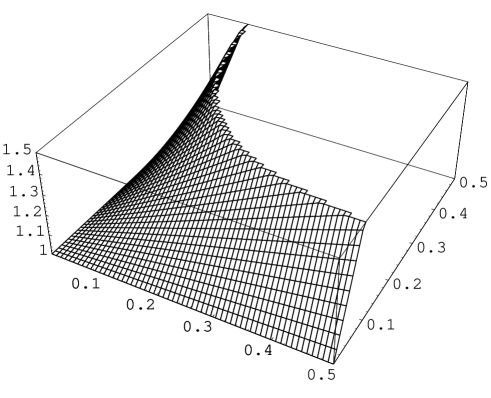
FIG. 1.: The energy per unit length, in unit of $M^{2}$ and at zeroth order, as function of ${\mathcal{X}}$ and $\Psi$ fermion densities plotted in unit of $M$, in the infinite string limit.

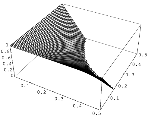
FIG. 2.: The tension, in unit of $M^{2}$ and at zeroth order, as function of ${\mathcal{X}}$ and $\Psi$ fermion densities plotted in unit of $M$, in the infinite string limit.

As expected from their analytical expressions in the infinite string limit, the energy per unit length is always positive and grows with both fermion densities, ${\mathcal{R}}_{\chi}$ and ${\mathcal{R}}_{\psi}$, whereas the tension always decreases and takes negatives values for large fermion densities. Obviously, in the case ${\mathcal{R}}_{\chi}={\mathcal{R}}_{\psi}=0$ there is no current along the string and we recover the Goto-Nambu case, $U=T=M^{2}$. The chiral case, where the fermionic current is lightlike, is obtained for ${\mathcal{R}}_{\chi}=0$, or ${\mathcal{R}}_{\psi}=0$, and also verifies $U=T=M^{2}$ as in the chiral scalar current case [28]. From Eq. (132), and in the infinite string limit, the densities for which the tension vanishes verify

$${\mathcal{R}}_{\chi}{\mathcal{R}}_{\psi}=\frac{M^{2}}{4\pi},$$ (134)

This curve separates the plane $({\mathcal{R}}_{\chi},{\mathcal{R}}_{\psi})$ in two regions where $T$ is positive near the origin, and negative on the other side (see Fig. 3). In the macroscopic formalism of Carter [19], the transverse perturbations propagation speed is given by $c_{T}^{2}=T/U$, and therefore the domains where $T<0$ correspond to strings which are always locally unstable with respect to transverse perturbations.

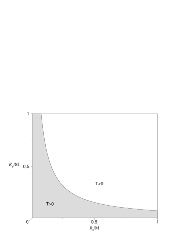
FIG. 3.: Sign of the tension in the $({\mathcal{R}}_{\chi}/M,{\mathcal{R}}_{\psi}/M)$ plane, in the infinite string limit. According to the macroscopic formalism, the string is unstable with respect to transverse perturbations for $T<0$.

The tension of the string becomes negative only for carrier densities close to the mass of the Goto-Nambu string $M$. For such currents, it is necessary to derive the backreaction in order to see how relevant it is for the energy per unit length and tension. Moreover, in a renormalizable model, the vacuum mass acquired by the fermions from their coupling to the Higgs field is less than the Goto-Nambu string mass, and thus, another quantum effects may take place before the negative tension is reached, like tunneling into massive states. Besides, note that $M$, the string unit of mass, arising from non-perturbative effects, may well be much larger than the Higgs mass, and so, it is expected that ${\mathcal{R}}_{\chi},{\mathcal{R}}_{\psi}\ll M$. Thus, the no-spring conjecture [18] proposed in the case of bosonic carrier presumably apply to the fermionic carrier case as well. Moreover, the zero mode vacuum effects on energy per unit length and tension appear clearly from Eq. (110) as additional string length. The corrected values of the equation of state are therefore obtained by replacing the physical length of the string, $L$, in Eq. (131) and Eq. (132), by an equivalent length, $L_{e}$ say, which verifies

$$\frac{1}{2L_{e}^{2}}=\frac{1}{2L^{2}}-\frac{1}{L_{v}^{2}}.$$ (135)

In the particular case where $L_{v}^{2}=6L^{2}$, it reads $L_{e}^{2}=(3/2)L^{2}$. On the other hand, the massive vacuum effects certainly shift in a different way $U$ and $T$ by a finite amount as previously discussed, but will not be considered in the following. In the next section, the backreaction is derived in the classical limit in order to find corrected values of energy per unit length and tension. Moreover we shall take care of the finite length of the string $L$, keeping in mind that its value, and consequently the value of $L_{e}$, have to be larger than $1/M$ since all physical values have been derived in the classical vortex background, i.e., the quantum effects of the Higgs field have been neglected.

C Backreaction

The existence of fermionic currents carrying gauge charge along the string gives rise to new gauge field components, $B_{t}$ and $B_{z}$, from the equations of motion (21). These, being coupled with the corresponding currents, provide additional terms in the energy momentum tensor (92). As a first step, the new gauge field components are computed numerically from the zero modes solutions of Eq. (32). The corrected equation of state is then analytically derived, the numerical dependencies having been isolated in model dependent coefficients.

1 Backreacted gauge fields

In order to compute the $B_{t}$ and $B_{z}$ fields at first order, we only need the zeroth order values of the zero modes and the vortex background. Let us introduce the dimensionless scaled fields and variables

$$\varphi=\eta H,\quad Q_{\theta}=Q\quad\textrm{and}\quad r=\frac{\varrho}{m_{h}},$$ (136)

with $m_{h}=\eta\sqrt{\lambda}$ the classical mass of the Higgs field. From the equation of motion (16), the orthoradial gauge field $Q$ and $H$ are solution of

$$\frac{d^{2}H}{d\varrho^{2}}+\frac{1}{\varrho}\frac{dH}{d\varrho} = \frac{HQ^{2}}{\varrho^{2}}+\frac{1}{2}H(H^{2}-1),$$ (137)

$$\frac{d^{2}Q}{d\varrho^{2}}-\frac{1}{\varrho}\ \frac{dQ}{d\varrho} = \frac{m_{b}^{2}}{m_{h}^{2}}H^{2}Q,$$ (138)

where $m_{b}=qc_{\phi}\eta$ is the classical mass of the gauge boson. The numerical solutions of these equations have been computed earlier by many people [13, 14] using relaxation methods [29]. They are presented in Fig. 4 for a specific (assumed generic) set of parameters.

FIG. 4.: The solutions of the field equations for the vortex background. The Higgs field, $H$, takes its vacuum expectation value at infinity and the gauge bosons condensate in the vortex.

In the same way, deriving Eq. (32) with respect to $\varrho$ yields the right component of the zero mode $Y$ as a solution of

$$\zeta_{1}^{\prime\prime}-\left(\frac{H^{\prime}}{H}+\frac{Q-n}{\varrho}\right)\zeta_{1}^{\prime} + \left(\frac{c_{\chi_{R}}}{c_{\phi}}\left[\frac{Q-n}{\varrho}\frac{H^{\prime}}{H}+\frac{Q-n}{\varrho^{2}}-\frac{Q^{\prime}}{\varrho}\right]\right.$$ (139)

$$- \left.\frac{c_{\chi_{L}}c_{\chi_{R}}}{c_{\phi}^{2}}\left(\frac{Q-n}{\varrho}\right)^{2}-\frac{m_{f}^{2}}{m_{h}^{2}}H^{2}\right)\zeta_{1}=0,$$ (140)

while the left one satisfies

$$i\frac{m_{f}}{m_{h}}H\zeta_{4} = \zeta_{1}^{\prime}-\frac{c_{\chi_{R}}}{c_{\phi}}\frac{Q-n}{\varrho}\zeta_{1},$$ (141)

where a prime indicates a derivation with respect to the dimensionless radial variable $\varrho$. The field $\Psi$ verifies similar equations with the transformation, $\zeta\rightarrow\xi$ and $c_{\chi}\rightarrow c_{\psi}$. The numerical integration has been performed with a relaxation method [29] and verified on the original system (32) with a shooting method. As a result, the normalized probability densities of the zero modes, $|X|^{2}$ and $|Y|^{2}$, are plotted in Fig. 5. The dimensionless radial functions $\tilde{f}_{\chi}$ and $\tilde{f}_{\psi}$ defined from Eq. (116) and Eq. (117) by

$$\tilde{f}_{\chi}=\frac{2\pi}{m_{h}^{2}}f_{\chi},\quad\textrm{and}\quad\tilde{f}_{\psi}=\frac{2\pi}{m_{h}^{2}}f_{\psi},$$ (142)

are plotted in Fig. 6. As expected, the fields are confined in the string core, and so will the corresponding fermionic currents.

Let us define the more relevant components of the backreacted gauge field, $\Delta B=B_{z}-B_{t}$ and $\Sigma B=B_{z}+B_{t}$, with the corresponding dimensionless scaled fields $\Delta\tilde{Q}$ and $\Sigma\tilde{Q}$ defined by

$$\Delta B=\left(\overline{\rho}_{\chi}-\rho_{\chi}\right)\frac{m_{b}^{2}}{\pi\eta^{2}}\frac{\Delta\tilde{Q}}{qc_{\phi}}, \Sigma B=-\left(\overline{\rho}_{\psi}-\rho_{\psi}\right)\frac{m_{b}^{2}}{\pi\eta^{2}}\frac{\Sigma\tilde{Q}}{qc_{\phi}}.$$ and (143)

The equations of motion (21) in the classical limit now reads

$$\Delta\tilde{Q}^{\prime\prime}+\frac{1}{\rho}\Delta\tilde{Q}^{\prime}-\frac{m_{b}^{2}}{m_{h}^{2}}H^{2}\Delta\tilde{Q}=\frac{\tilde{f}_{\chi}}{qc_{\phi}}, \Sigma\tilde{Q}^{\prime\prime}+\frac{1}{\rho}\Sigma\tilde{Q}^{\prime}-\frac{m_{b}^{2}}{m_{h}^{2}}H^{2}\Sigma\tilde{Q}=\frac{\tilde{f}_{\psi}}{qc_{\phi}}.$$ and (144)

As for fermions, these new gauge fields get their masses from coupling with the Higgs field, and therefore have non-zero mass outside the string core. Moreover, they are generated by fermionic massless currents confined in the core, therefore they also condense in and do not lead to new long-range effects. The solutions of these equations (144) have been obtained using, once again, a relaxation method [29] and are represented in Fig. 7. Note that owing to the scaled field $\Delta\tilde{Q}$ and $\Sigma\tilde{Q}$, we have separated the numerical dependence in the gauge field and currents from the fermion densities content [see Eq. (143)].

FIG. 5.: The normalized probability densities of the zero modes, $|X|^{2}$ and $|Y|^{2}$. The rapid decay far from the string core reflects the bound state nature of the condensates.

FIG. 6.: The dimensionless radial current functions $\tilde{f}_{\chi}$ and $\tilde{f}_{\psi}$. They can be viewed as the effective transverse density charge carried by the fermion currents. Their sign results in the initial choice of each conserved fermion gauge charge.

FIG. 7.: The dimensionless backreacted gauge fields $\Delta\tilde{Q}$ and $\Sigma\tilde{Q}$, generated by the fermion currents. They do not lead to new long-range effects since they acquire non-zero mass outside the string core due to their coupling with the Higgs fields.

Up to now, we have computed the fermionic gauge currents along the string as well as the component $B_{t}$ and $B_{z}$, so that the backreaction correction to the energy momentum tensor is computable from Eq. (92). As in the previous section, the energy per unit length and tension can be derived in the preferred frame where the stress tensor is diagonal, but now we have to find the eigenvalues of the full two-dimensional energy momentum tensor $\overline{T}^{\alpha\beta}_{b.r.}+\langle\overline{T}^{\alpha\beta}\rangle$, with

$$\overline{T}^{\alpha\beta}_{b.r.}=\int{r\,{\mathrm{d}}r\,{\mathrm{d}}\theta\,T^{\alpha\beta}_{b.r.}}$$ (145)

2 Energy per unit length and tension with backreaction

Using the dimensionless field, $\Delta\tilde{Q}$ and $\Sigma\tilde{Q}$, with the expressions of the currents given in equations (114) and (115), one gets, after some algebra, the full expression of the stress tensor with corresponding eigenvalues

$$\widehat{U} = M^{2}-I(\Theta_{\chi},\Theta_{\psi})\widehat{{\mathcal{R}}}_{\chi}\widehat{{\mathcal{R}}}_{\psi}+4\pi\sqrt{\left(\widehat{{\mathcal{R}}}_{\chi}^{2}-\frac{1}{2L_{e}^{2}}\right)\left(\widehat{{\mathcal{R}}}_{\psi}^{2}-\frac{1}{2L_{e}^{2}}\right)},$$ (146)

$$\widehat{T} = M^{2}-I(\Theta_{\chi},\Theta_{\psi})\widehat{{\mathcal{R}}}_{\chi}\widehat{{\mathcal{R}}}_{\psi}-4\pi\sqrt{\left(\widehat{{\mathcal{R}}}_{\chi}^{2}-\frac{1}{2L_{e}^{2}}\right)\left(\widehat{{\mathcal{R}}}_{\psi}^{2}-\frac{1}{2L_{e}^{2}}\right)},$$ (147)

with the scaled state parameters

$$\widehat{{\mathcal{R}}}_{\chi} = {\mathcal{R}}_{\chi}\sqrt{1-\frac{m_{b}^{2}}{2\pi^{2}\eta^{2}}\left(I_{\Delta\chi}-I_{\Delta 2}\right)\sin^{2}{\left(\Theta_{\chi}-\frac{\pi}{4}\right)}},$$ (148)

$$\widehat{{\mathcal{R}}}_{\psi} = {\mathcal{R}}_{\psi}\sqrt{1-\frac{m_{b}^{2}}{2\pi^{2}\eta^{2}}\left(I_{\Sigma\psi}-I_{\Sigma 2}\right)\sin^{2}{\left(\Theta_{\psi}-\frac{\pi}{4}\right)}},$$ (149)

and the function $I(\Theta_{\chi},\Theta_{\psi})$ defined by

$$I(\Theta_{\chi},\Theta_{\psi})=\frac{m_{b}^{2}}{\pi\eta^{2}}\frac{\left(I_{\Sigma\chi}+I_{\Delta\psi}\right)\sin{\left(\Theta_{\chi}-\frac{\pi}{4}\right)}\sin{\left(\Theta_{\psi}-\frac{\pi}{4}\right)}}{\sqrt{1-\frac{m_{b}^{2}}{2\pi^{2}\eta^{2}}\left(I_{\Delta\chi}-I_{\Delta 2}\right)\sin^{2}{\left(\Theta_{\chi}-\frac{\pi}{4}\right)}}\sqrt{1-\frac{m_{b}^{2}}{2\pi^{2}\eta^{2}}\left(I_{\Sigma\psi}-I_{\Sigma 2}\right)\sin^{2}{\left(\Theta_{\psi}-\frac{\pi}{4}\right)}}}.$$ (150)

The numerical integrations previously carried out appear through pure numbers which depend only on the model parameters. The coupling $B_{\mu}j^{\mu}$ leads to the following quantities

$$I_{\Sigma\chi}=-2\int{\,\varrho\,{\mathrm{d}}\varrho\,\Sigma\tilde{Q}(\varrho)\frac{\tilde{f}_{\chi}(\varrho)}{qc_{\phi}}}, I_{\Delta\psi}=-2\int{\,\varrho\,{\mathrm{d}}\varrho\,\Delta\tilde{Q}(\varrho)\frac{\tilde{f}_{\psi}(\varrho)}{qc_{\phi}}},$$ (151)

$$I_{\Sigma\psi}=-2\int{\,\varrho\,{\mathrm{d}}\varrho\,\Sigma\tilde{Q}(\varrho)\frac{\tilde{f}_{\psi}(\varrho)}{qc_{\phi}}}, I_{\Delta\chi}=-2\int{\,\varrho\,{\mathrm{d}}\varrho\,\Delta\tilde{Q}(\varrho)\frac{\tilde{f}_{\chi}(\varrho)}{qc_{\phi}}},$$ (152)

while the kinetic contribution of the new gauge fields appears through

$$I_{\Delta 2}=\int{\,\varrho\,{\mathrm{d}}\varrho\,\left(\partial_{\varrho}\Delta\tilde{Q}(\varrho)\right)^{2}}, I_{\Sigma 2}=\int{\,\varrho\,{\mathrm{d}}\varrho\,\left(\partial_{\varrho}\Sigma\tilde{Q}(\varrho)\right)^{2}}.$$ (153)

By means of the equations of motion (144) and the constant sign of $\Delta\tilde{Q}$ and $\Sigma\tilde{Q}$, $I_{\Delta\chi}$ and $I_{\Sigma\psi}$ are found to be always positive. Intuitively, as in electromagnetism, the gauge field generated from charge currents tends to resist to the currents which give birth to it. In our case, the backreaction actually damps the weight of the charge carriers in the energy per unit length and tension. In fact, the relevant state parameters are now $\widehat{{\mathcal{R}}}$ instead of ${\mathcal{R}}$ with $\widehat{{\mathcal{R}}}<{\mathcal{R}}$ since $I_{\Delta\chi}$ and $I_{\Sigma\psi}$ are positive. Moreover, numerical calculations show that the kinetic contribution numbers (153) are always one order of magnitude smaller than those resulting in the coupling between gauge fields and currents (151), as expected for reasonable backreacted gauge field since they only involve the square gradient of these fields [see Eq. (153)]. However, there is an additional term involving new dependence in the asymmetry between particles and anti-particles through the $I(\Theta_{\chi},\Theta_{\psi})$ function. In order to understand this point physically, let us derive the magnitude of the gauge current carried by the fermions. From Eq. (114) and Eq .(115), once the transverse coordinates have been integrated over, the dimensionless magnitude reads

$$\tilde{\overline{j}}^{2}=2(2qc_{\phi})^{2}\frac{\tilde{F}_{\chi}\tilde{F_{\psi}}\sin{\left(\Theta_{\chi}-\frac{\pi}{4}\right)}\sin{\left(\Theta_{\psi}-\frac{\pi}{4}\right)}\widehat{{\mathcal{R}}}_{\chi}\widehat{{\mathcal{R}}}_{\psi}}{\sqrt{1-\frac{m_{b}^{2}}{2\pi^{2}\eta^{2}}\left(I_{\Delta\chi}-I_{\Delta 2}\right)\sin^{2}{\left(\Theta_{\chi}-\frac{\pi}{4}\right)}}\sqrt{1-\frac{m_{b}^{2}}{2\pi^{2}\eta^{2}}\left(I_{\Sigma\psi}-I_{\Sigma 2}\right)\sin^{2}{\left(\Theta_{\psi}-\frac{\pi}{4}\right)}}},$$ (154)

with the dimensionless constants are

$$\tilde{F}_{\chi}=\int{\,\varrho\,{\mathrm{d}}\varrho\,\frac{\tilde{f}_{\chi}(\varrho)}{qc_{\phi}}}, \tilde{F}_{\psi}=\int{\,\varrho\,{\mathrm{d}}\varrho\,\frac{\tilde{f}_{\psi}(\varrho)}{qc_{\phi}}}.$$ and (155)

These numbers can be viewed as the effective charge carried by the fermionic gauge currents since

$$\frac{\tilde{\overline{j}}^{2}}{(2qc_{\phi})^{2}\tilde{F_{\chi}}\tilde{F_{\psi}}}=\frac{\overline{{\mathcal{C}}}^{2}}{4}.$$ (156)

The function $I(\Theta_{\chi},\Theta_{\psi})$ therefore verifies

$$I(\Theta_{\chi},\Theta_{\psi})\widehat{{\mathcal{R}}}_{\chi}\widehat{{\mathcal{R}}}_{\psi}=\frac{I_{\Sigma\chi}+I_{\Delta\psi}}{8\pi\tilde{F}_{\chi}\tilde{F}_{\psi}}\tilde{\overline{j}}^{2},$$ (157)

and, as before, according to Eq. (144), $(I_{\Sigma\chi}+I_{\Delta\psi})/(\tilde{F}_{\chi}\tilde{F}_{\psi})$ is always positive, so the sign of $I$ directly reflects the spacelike or timelike nature of the current. Thus, in addition to the backreaction damping effect, there is a correction to the energy per unit length and tension directly proportional to the magnitude of the fermionic current. Note that this effect appears as a correction due to backreaction and not, as it is the case for cosmic string with bosonic current carriers, at the zeroth order [14].

3 Equation of state with backreaction

Unfortunately, the corrected expressions of the line density energy and tension involve four independent state parameters, and consequently are not easily representable. However, they can be studied as functions of the damped fermion densities $\widehat{{\mathcal{R}}}$, modified only by the function $I(\Theta_{\chi},\Theta_{\psi})$ which quantifies the efficiency of the fermionic currents in generating backreacted gauge fields. In this way, the comparison with the zeroth order case is all the more so easy.

The study of the surfaces defined by $\widehat{U}$ and $\widehat{T}$ in the plane $(\widehat{{\mathcal{R}}}_{\chi},\widehat{{\mathcal{R}}}_{\psi})$ is less canonical than at zeroth order. Three critical values of the function $I$ are found to modify the behaviors of the tension and energy per unit length, namely, $-4\pi$, $0$, and $4\pi$. However, only small values of $I$ are reasonable in this model as it is discussed in the next section. This analysis is consequently constraints to values of $|I|<4\pi$.

a Energy per unit length.

The line density energy follows different behaviors according to the value of $I$.

The first and simplest case $I<0$, obtained for spacelike fermionic gauge currents, is very similar to the zeroth order case, and the energy per unit length just grows a bit faster with the damped fermion densities $\widehat{{\mathcal{R}}}_{\chi}$ and $\widehat{{\mathcal{R}}}_{\psi}$, as on Fig. 8.

For timelike currents, $I>0$, we find that the backreaction damps the growth of the density line energy with the fermion densities. As a result the line density energy seems to decrease in some regions, and the stationary curves of $\widehat{U}$ with respect to $\widehat{{\mathcal{R}}}_{\chi}$ are given, from Eq. (146), by

$$\frac{\partial{\widehat{U}}}{\partial\widehat{{\mathcal{R}}}_{\chi}}=0 \Leftrightarrow \widehat{{\mathcal{R}}}_{\psi}=\frac{2\pi}{L_{e}}\widehat{{\mathcal{R}}}_{\chi}\sqrt{\frac{2}{\frac{I^{2}}{2L_{e}^{2}}+(16\pi^{2}-I^{2})\widehat{{\mathcal{R}}}_{\chi}^{2}}},$$ (158)

and thanks to the symmetry between $\widehat{{\mathcal{R}}}_{\chi}$ and $\widehat{{\mathcal{R}}}_{\psi}$, similar equations are obtained for $\partial\widehat{U}/\partial\widehat{{\mathcal{R}}}_{\psi}=0$. Finally, the variation domains of the line density energy are represented in Fig. 9 for $0<I<4\pi$. The first discrete values of the fermion densities (the length of the string is finite) have been represented by dots in the $(\widehat{{\mathcal{R}}}_{\chi}$,$\widehat{{\mathcal{R}}}_{\psi})$-plane, and as can be seen in Fig. 9, for reasonable values of $I$, there is no available quantum state inside the tiny decreasing regions. Consequently, the density line energy always grows with the fermions densities and remains positive. Since the stationary curves of $\widehat{U}$ are asymptotically proportional to $1/L_{e}<1/L$ [see Eq. (158)], they coincide with the axis in the infinite string limit. The surface describing $\widehat{U}(\widehat{{\mathcal{R}}}_{\chi},\widehat{{\mathcal{R}}}_{\psi})$ has also been plotted in Fig. 9 in unit normalized to $M^{2}$, and for minimal acceptable value of $L_{e}=10/M$ just in order to show the influence of the finite length.

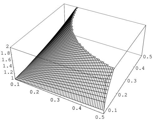
FIG. 8.: The energy per unit length in unit of $M^{2}$ as function of $\widehat{{\mathcal{R}}}_{\chi}/M$ and $\widehat{{\mathcal{R}}}_{\psi}/M$, for spacelike currents with $I(\Theta_{\chi},\Theta_{\psi})<0$. The influence of the finite length of the string just appears near the axes.

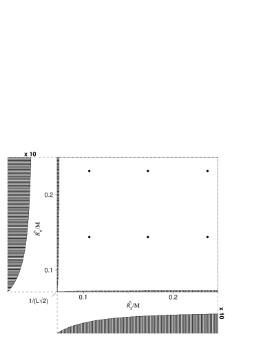
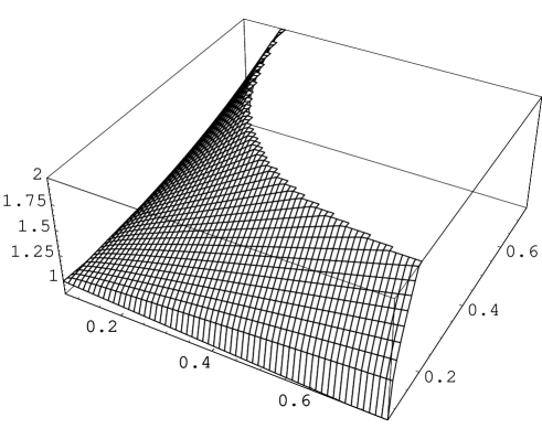
FIG. 9.: Variation domains of the energy per unit length, plotted in unit of $M^{2}$, in the $(\widehat{{\mathcal{R}}}_{\chi}/M,\widehat{{\mathcal{R}}}_{\psi}/M)$ plane for timelike currents with $0<I<4\pi$. The vertical hatched regions define domains where the line density energy could decrease with $\widehat{{\mathcal{R}}}_{\chi}$ whereas the horizontal ones are regions where the line density energy could decrease with $\widehat{{\mathcal{R}}}_{\psi}$. On one hand, these domains are asymptotically limited by the curves $\widehat{{\mathcal{R}}}=(2\pi/L_{e})\sqrt{2/(16\pi^{2}-I^{2})}$ and therefore coincide with the axis for large values of $L_{e}$. On the other hand, for reasonable values of $I\ll 4\pi$, there is no accessible quantum state inside, the first one being shown as a dot. As a result the energy per unit length always grows with the parameters $\widehat{{\mathcal{R}}}$ and is always positive.

b Tension.

The study of the tension with respect to the fermion densities is performed in the same way. As before the stationary curves of $\widehat{T}$ with respect to $\widehat{{\mathcal{R}}}_{\chi}$ or $\widehat{{\mathcal{R}}}_{\psi}$ are found from Eq. (147), and follow the same equation as those of the energy per unit length in Eq. (158), although the variation domains are not the same and have been plotted in Fig. 11 for different values of the function $I$.

For timelike fermionic gauge current, $I>0$, the tension decreases faster than in the zeroth order case, with the damped fermionic densities $\widehat{{\mathcal{R}}}_{\chi}$ and $\widehat{{\mathcal{R}}}_{\psi}$ as on Fig. 10, and reaches negative values at large densities (see Fig. 12). The backreaction just increases the slope of the surface, and thus, the negative values are reached more rapidly. As for the energy per unit length, the equivalent length was chosen equal to $L_{e}=10/M$ in the following figures.

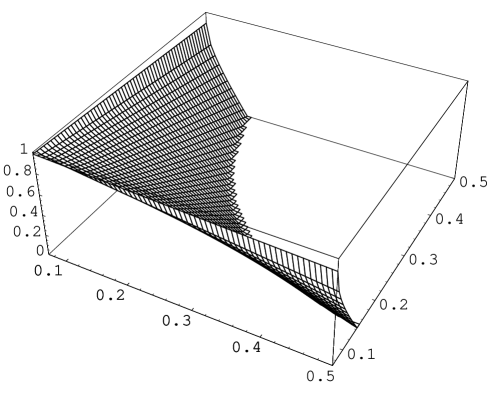
FIG. 10.: The tension for timelike currents with $I>0$, plotted in unit of $M^{2}$ in the $(\widehat{{\mathcal{R}}}_{\chi}/M,\widehat{{\mathcal{R}}}_{\psi}/M)$ plane. Note the shift near the axes due to the finite length of the string.

For spacelike fermionic gauge currents, $-4\pi<I<0$, the backreaction damps the decrease of the tension with respect to the damped fermion densities. There are also tiny regions near the axis, with areas inversely proportional to $L_{e}$, and where $\widehat{T}$ could grow with respect to one of the state parameters $\widehat{{\mathcal{R}}}_{\chi}$ or $\widehat{{\mathcal{R}}}_{\psi}$ (see Fig. 11). As previously, for reasonable values of $I$, the first discrete values of the parameters are out of these domains, and the tension always decreases with both fermion densities. Finally, the tension reaches negative values at large damped fermion densities (see Fig. 12).

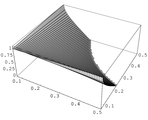
FIG. 11.: Variation domains of the tension, plotted in unit of $M^{2}$, for spacelike currents with $-4\pi<I<0$, in the $(\widehat{{\mathcal{R}}}_{\chi}/M,\widehat{{\mathcal{R}}}_{\psi}/M)$ plane. These regions have the same geometrical properties as the line density energy ones in Fig. 9, but this time, the zones with vertical hatches are domains where $\widehat{T}$ could grow with respect to $\widehat{{\mathcal{R}}}_{\chi}$, whereas the horizontal ones correspond to growth with respect to $\widehat{{\mathcal{R}}}_{\psi}$. For reasonable values of $I$, the discrete values of $\widehat{{\mathcal{R}}}$, represented by dots, are out of these regions, and the tension always decrease with both fermion densities.

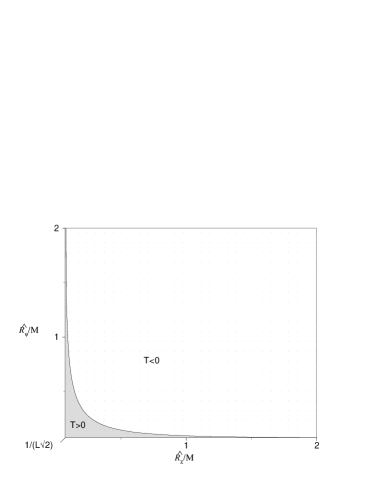
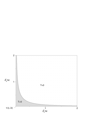
FIG. 12.: Sign of the tension for timelike currents with $I>0$, and spacelike currents with $-4\pi<I<0$, the curves have been plotted with $L_{e}=10/M$ in aim at clearly separating the various regions. In the timelike case, the domain where the tension is positive is closed, the null tension curves intersecting the axes at $\widehat{{\mathcal{R}}}=\sqrt{2}L_{e}M^{2}/I$, whereas for spacelike currents, the null tension curves tends asymptotically to $\widehat{{\mathcal{R}}}=(2\pi/L_{e})\sqrt{2/(16\pi^{2}-I^{2})}$. Recall that the regions where $T<0$ are unstable with respect to transverse string perturbations according to the macroscopic formalism.

4 Relevant values of the parameters

The previous derivation of the backreaction is built on the classical vortex background and it is acceptable only if the backreacted gauge fields do not perturb appreciably the Higgs and orthoradial gauge fields profiles (see Fig. 4). From Eq. (16), it will be the case only if $Q^{t}Q_{t}$ and $Q^{z}Q_{z}$ can be neglected compared to $Q^{\theta}Q_{\theta}$. From Eq. (143), and $Q_{\theta}Q^{\theta}\sim m_{b}^{2}$, this condition reads

$$\frac{(qc_{\phi})^{2}\Delta B\Sigma B}{Q_{\theta}Q^{\theta}}\sim\frac{{\mathcal{R}}_{\chi}{\mathcal{R}}_{\psi}\sin{\left(\Theta_{\chi}-\frac{\pi}{4}\right)}\sin{\left(\Theta_{\psi}-\frac{\pi}{4}\right)}}{\pi\eta^{2}}\frac{m_{b}^{2}}{\pi\eta^{2}}\Delta\tilde{Q}\Sigma\tilde{Q} \ll 1,$$ (159)

or as function of $I(\Theta_{\psi},\Theta_{\chi})$ and the damped fermion densities,

$$I(\Theta_{\chi},\Theta_{\psi})\frac{\widehat{{\mathcal{R}}}_{\chi}\widehat{{\mathcal{R}}}_{\psi}}{\pi\eta^{2}} \ll 1.$$ (160)

This condition is satisfied for damped fermion densities small compared to the string energy scale, or for tiny values of the function $I(\Theta_{\psi},\Theta_{\chi})$. Moreover, the backreacted gauge fields need to be small in order to no perturb significantly the zero modes. From the equations of motion (22) and (24), this condition leads to $\Delta B,\Sigma B\ll{\mathcal{R}}$ and from Eq. (143) to

$$\frac{m_{b}^{2}}{\eta^{2}}\frac{c_{\psi(\chi)}}{c_{\phi}}\Sigma(\Delta)\tilde{Q}(0)\ll 1.$$ (161)

On the other hand, the maximum value of $I$ in Eq. (150) is clearly obtained when there are only particles or anti-particles trapped in the string ($\Theta=0$ or $\Theta=\pi$), and deriving the order of magnitude of the numerical integral in Eq. (151), using equations (144) and (116)-(117), one shows that the large values of $I$ (as $I>4\pi$) can only be obtained for model parameters which verify

$$\frac{m_{b}^{2}}{\eta^{2}}\frac{c_{\psi(\chi)}}{c_{\phi}}\Sigma(\Delta)\tilde{Q}(0)>1.$$ (162)

As a result, in order for the backreacted gauge fields not to modify the equations of motion of the fermions at first order, the function $I$ has to be much smaller than $4\pi$. If it is not the case, then the previous zero modes are no longer valid solutions and the relevant equations of motion, in the case of the $\Psi$ fermions, now read, from Eq. (22)

$$\left\{\begin{array}[]{lll}\vspace{4pt}\displaystyle\left(\frac{{\mathrm{d}}\xi_{1}}{{\mathrm{d}}r}+\frac{1}{r}\left[-qc_{\psi_{R}}B(r)+m_{1}\right]\xi_{1}(r)\right)-ig\varphi(r)\xi_{4}(r)&=&i[\mp(k+\omega)-qc_{\psi_{R}}\Delta B]\xi_{2}(r),\\ \vspace{4pt}\displaystyle\left(\frac{{\mathrm{d}}\xi_{2}}{{\mathrm{d}}r}+\frac{1}{r}\left[qc_{\psi_{R}}B(r)-m_{2}\right]\xi_{2}(r)\right)-ig\varphi(r)\xi_{3}(r)&=&i[\pm(k-\omega)-qc_{\psi_{R}}\Sigma B]\xi_{1}(r),\\ \vspace{4pt}\displaystyle\left(\frac{{\mathrm{d}}\xi_{3}}{{\mathrm{d}}r}+\frac{1}{r}\left[-qc_{\psi_{L}}B(r)+m_{3}\right]\xi_{3}(r)\right)+ig\varphi(r)\xi_{2}(r)&=&i[\mp(k-\omega)-qc_{\psi_{L}}\Sigma B]\xi_{4}(r),\\ \displaystyle\left(\frac{{\mathrm{d}}\xi_{4}}{{\mathrm{d}}r}+\frac{1}{r}\left[qc_{\psi_{L}}B(r)-m_{4}\right]\xi_{4}(r)\right)+ig\varphi(r)\xi_{1}(r)&=&i[\pm(k+\omega)-qc_{\psi_{L}}\Delta B]\xi_{3}(r),\end{array}\right.$$ (163)

where the angular dependence has not been written owing to Eq. (31) and assuming $m_{1}=m_{3}+n$. The zero modes seem to acquire an effective mass proportional to $\Delta B$ or $\Sigma B$. More precisely, they are no longer eigenstates of the $\gamma^{0}\gamma^{3}$ operator since new spinor components appear [$\xi_{1}$, $\xi_{4}$ here, see Eq. (32) and Eq. (33)]. It is clearly a second order effect since the gauge coupling constant $q$ can be removed in the previous equations (163) using Eq. (143) and assuming

$$\xi=X+q^{2}\delta\xi,$$ (164)

with $X$ the zero mode solution $k=-\omega$ for $\Psi$ fermions [see Eq. (42)], and $q^{2}\delta\xi$ the perturbation induced by the backreaction [35]. As a result, for strong backreaction, the semi-classical approach can no longer be used, since such second order effects appear as the semi-classical manifestations of the one loop quantum corrections, and thus, only a full quantum theory would be well defined. However, if there is only one kind of fermion trapped in the string, $\Psi$ say, the zero modes are not affected by the backreaction since $\Delta B$ is only generated from the ${\mathcal{X}}$ current, and therefore vanishes [see Eq. (144)], so $\xi=X$ is always solution of the equations of motion (163), and identically for the ${\mathcal{X}}$ zero modes alone [34]. Note, that there is no contradiction with the usual index theorem since it is derived for Dirac operators, and thus without backreacted fields. This just shows that the modes propagating in the vortex with strong backreacted gauge fields are no longer well described by the usual zero modes. Physically, it might be the signature of a tunneling of the zero modes to another states. The massive modes which have not been considered here could be more relevant in such cases.

On the other hand, the shape of the string might allow the fermion densities $\widehat{{\mathcal{R}}}_{\chi}$ and $\widehat{{\mathcal{R}}}_{\psi}$ to reach the tiny regions where the energy decreases with one of them (see Fig. 9), by means of the zero mode vacuum quantum effects. The present toy model does not involve the effect of the radius of curvature $R$ of the string, and it is reasonable that the contribution of the zero mode vacuum to the energy per unit length involves $R$ through a redefinition of $L_{e}$. If $L_{e}$ becomes smaller than $L$, the first discrete values of the fermion densities could be inside the hatched regions in Fig. 9, since the discrete values of the fermion densities only depend on the physical length of the string $L$. Note that it would therefore be necessary that the zero mode vacuum energy is negative, which is not the case without curvature in the simple framework of section IV B 1. Such effects could be relevant for vorton stability, as, for a small radius of curvature, the string could become unstable to fermion condensation.

Finally, the model can be used only at the tree order, and the conditions (160) and (161) are the validity criteria of the above derivations.

VI Comparison with the scalar case

Owing to the fermionic two-dimensional quantization along the string, the energy per unit length and the tension of a string carrying massless fermionic currents have been derived up to the first order in backreaction corrections. The state of the string is found to be well defined with four state parameters which are the densities of each fermion trapped in the string, and asymmetry angles between particles and anti-particles in each fermion family. It seems quite different than the bosonic charge carriers case, where the current magnitude is the only relevant state parameter [14], however, this is the result of the allowed purely classical approach where the superposition of many quantum states can be view as only one classical state owing to the bosonic nature of the charge carriers. As a result, there is a degeneracy between the number of bosons trapped in the string and the charge current. The quantization introduced to deal with fermions naturally leads to separate the charge current from the particle current through the existence of anti-particle exitations. Moreover, the magnitude of the current can only modify the equation of state at non-zeroth order because the chiral nature of fermions trapped in the string requires simultaneous exitations between the two families to lead to non-lightlike charge currents.

Nevertheless, some global comparisons can be made with the scalar case. First, for reasonable values of $I\ll 4\pi$, the energy per unit length grows with the fermionic densities, whereas the tension decreases with them. However, note the relevant parameter for the change in behaviors of the tension and line density energy is the function $I(\Theta_{\chi},\Theta_{\psi})$ instead of the current magnitude in the scalar case. As it was said, $I$ quantifies, through the asymmetry between the number of particles and anti-particles trapped in the string, the efficiency of the charge current per particle to be timelike or spacelike. The more positive is $I$, the more timelike the fermionic charge current per particle will be, and conversely the more negative $I$ is, the more spacelike it will be. Once again, this difference with the scalar case appears as a result of the degeneracy breaking between particle current and charge current due to the fermionic nature of the charge carriers.

The stability of the string with respect to transverse perturbations is given from the macroscopic formalism by the sign of the tension (for line density energy positive) [19], and we find that instabilities always occur for densities roughly close to $M/\sqrt{4\pi+I}$, in finite domain for timelike current, in infinite one for spacelike currents with $-4\pi<I<0$. Another new results are obtained from the multi-dimensional properties of the equation of state, in particular the problem of stability with respect to longitudinal perturbations differs from the scalar barotropic case where the longitudinal perturbations propagation speed is given by $c_{L}^{2}=-dT/dU$ [19], and therefore its two-dimensional form has to be derived to conclude on these kinds of instabilities. Nevertheless, by analogy with the scalar case, since, in the non-perturbed case and in the infinite string limit, the equation of state verifies $U+T=2M^{2}$ [22], the longitudinal perturbation propagation speed might be close to the speed of the light, even with small backreaction, and therefore, only transverse stability would be relevant in macroscopic string stability with massless fermionic currents.

VII Conclusion

The energy per unit length and the tension of a cosmic string carrying fermionic massless currents were derived in the frame of the Witten model in the neutral limit. Contrary to bosonic charge carriers, the two-dimensional quantization required to deal with fermions, leads to more than one state parameter in order to yield a well-defined equation of state. They can be chosen, at zeroth order, as fermion densities trapped in the string regardless of charge conjugation. The minimal backreaction correction appears through the fermionic charge current magnitude which involves the asymmetry angles between the number of particles and anti-particles trapped in the string, and which might be identified with the baryonic number of the plasma in which the string was formed during the phase transition. As a result, it is shown that fermionic charge currents can be lightlike, spacelike as well as timelike. Moreover the line energy density and the tension evolve globally as in the bosonic charge carriers case, but it was found that the tension can take negative values in extreme regions where the fermion densities are close to the string mass, and where the string is therefore unstable with respect to transverse perturbations according to the macroscopic formalism.

The present model has been built on the generic existence of fermionic zero modes in the string and follows only a semi-classical approach. It is no longer valid for higher corrections in the backreaction when they modify notably the vortex background and seem to give effective mass to the previous zero modes. It may be conjectured, at this stage, that in a full quantum theory, the quantum loop corrections give mass to the zero modes for high currents and consequently might lead to their decay by the mean of massive states. Only chiral charge currents could be stable on cosmic string carrying large fermionic massless currents in such a case. Another possible effect, relevant for vortons stability, may be expected for loops with small radius of curvature, by means of the vacuum effects which could render the loop unstable to fermion condensation.

It will be interesting to quantify such modifications on the equation of state in future works, as the effects of worldsheet curvature, and the modification of the density line energy and tension by the massive bound states. The field of validity of the model could therefore be extended to higher energy scales which would be more relevant for vortons and string formation.

- [1] T.W.B. Kibble, Phys. Rep. 67, 183 (1980).
- [2] E. Witten, Nucl. Phys. B249, 557, (1985).
- [3] J. P. Ostriker, C. Thompson, E. Witten Phys. Lett. B 180, 231 (1986).
- [4] D. P. Bennett, F. R. Bouchet, A. Stebbins, Nature 335, 410 (1988); D. P. Bennett, F. R. Bouchet, Phys. Rev. D41, 2408 (1990); L. Perivolaropoulos, Ap. J. 451, 429 (1995); B. Allen, R. R. Caldwell, S. Dodelson, L. Knox, E. P. S. Shellard, A. Stebbins, Phys. Rev. Lett.79, 2624 (1997).
- [5] P. P. Avelino, E. P. S. Shellard, J. H. P. Wu, B. Allen, Phys. Rev. D60, 023511 (1999); J. H. P. Wu, P. P. Avelino, E. P. S. Shellard, B. Allen, astro-ph/9812156 (1998); C. Contaldi, M. Hindmarsh, J. Magueijo, Phys. Rev. Lett.82, 679 (1999).
- [6] F. R. Bouchet, P. Peter, A. Riazuelo, M. Sakellariadou, Phys. Rev. Lett.(2000), to appear.
- [7] P. De Bernardis et al., Nature404, 955 (2000).
- [8] T. Goto, Prog. Theor. Phys. 46, 1560 (1971); Y. Nambu, Phys. Rev. D10, 4262 (1974).
- [9] R.L. Davis, Phys. Rev. D38, 3722 (1988).
- [10] R. Brandenberger, B. Carter, A. C. Davis, M. Trodden, Phys. Rev. D54, 6059 (1996).
- [11] R. L. Davis, Phys. Rev. D36, 2267 (1987); C. T. Hill, L. M. Widrow, Phys. Lett. B 189, 17 (1987); M. Hindmarsh, Phys. Lett. B 200, 429 (1988).
- [12] A. E. Everett, Phys. Rev. Lett.61, 1807 (1988); J. Ambjørn, N. K. Nielsen, P. Olesen, Nucl. Phys. B 310, 625 (1988).
- [13] A. Babul, T. Piran, D. N. Spergel, Phys. Lett. B 202, 307 (1988).
- [14] P. Peter, Phys. Rev. D45, 1091 (1992).
- [15] P. Peter, Phys. Rev. D46, 3335 (1992).
- [16] J. Garriga, P. Peter, Class. Quantum Grav. 11, 1743 (1994).
- [17] P. Peter, Class. Quantum Grav. 11, 131 (1994); P. Peter, D. Puy, Phys. Rev. D48, 5546 (1993).
- [18] P. Peter, Phys. Rev. D47, 3169 (1993).
- [19] B. Carter, Phys. Lett. B 224, 61 (1989); B. Carter, Phys. Lett. B 228, 466 (1989); B. Carter, Nucl. Phys. B 412, 345 (1994); B. Carter, P. Peter, A. Gangui, Phys. Rev. D55, 4647 (1997); A. Gangui, P. Peter, C. Boehm Phys. Rev. D57, 2580 (1998).
- [20] B. Carter, P. Peter, Phys. Rev. D52, R1744 (1995).
- [21] B. Carter, P. Peter, Phys. Lett. B 466, 41 (1999).
- [22] P. Peter, C. Ringeval, hep-ph/0011308 (2000), submitted to Phys. Lett. B.
- [23] X. Martin, P. Peter, Phys. Rev. D51 4092 (1995).
- [24] B. Carter, X. Martin, Ann. of Physics 227, 151 (1993); X. Martin, Phys. Rev. D50, 7479 (1994).
- [25] S. C. Davis, W. B. Perkins, A. C. Davis, Phys. Rev. D62, 043503 (2000).
- [26] P. W. Higgs, Phys. Rev. 145, 1156 (1966).
- [27] R. Jackiw, P. Rossi, Nucl. Phys. B 190, 681 (1981).
- [28] B. Carter, P. Peter, Phys. Lett. B 466, 41-49 (1999).
- [29] S. L. Adler, T. Piran, Rev. Mod. Phys. 56, 1 (1984).
- [30] N. K. Nielsen, P. Olesen, Nucl. Phys. B 291, 829 (1987).
- [31] S. A. Fulling, Phys. Rev. D7 2850 (1973).
- [32] B. S. Kay, Phys. Rev. D20 3052 (1979).
- [33] N. D. Birrell, P. C. W. Davies, Quantum fields in curved space (Cambridge University Press, 1994).
- [34] J. M. Moreno, D. H. Oaknin, M. Quirós, Phys. Lett. B 347, 332 (1995).
- [35] C. Ringeval, in preparation.
- [36] B. Carter, private communication.