Measuring sparticle masses in non-universal string inspired models at the LHC

Abstract:

We demonstrate that some of the suggested five supergravity points for study at the LHC could be approximately derived from perturbative string theories or M-theory, but that charge and colour breaking minima would result. As a pilot study, we then analyse a perturbative string model with non-universal soft masses that are optimised in order to avoid global charge and colour breaking minima. By combining measurements of up to six kinematic edges from squark decay chains with data from a new kinematic variable, designed to improve slepton mass measurements, we demonstrate that a typical LHC experiment will be able to determine squark, slepton and neutralino masses with an accuracy sufficient to permit an optimised model to be distinguished from a similar standard SUGRA point. The technique thus generalizes SUSY searches at the LHC.

1 Introduction

The purpose of this work is to extend the discussion of LHC supersymmetry (SUSY) searches to include string models. We begin by discussing whether string models can be used to motivate previous work on LHC SUSY searches, and then suggest a well-motivated non-universal string model for a new pilot study. We go on to examine how the SUSY particles can be detected and how the model can be distinguished from a similar well studied supergravity (SUGRA) model. We reconstruct sparticle masses by looking for kinematic edges in ${\tilde{{q}}}_{L}\rightarrow{{\tilde{{\chi}}}^{0}_{2}}q\rightarrow{\tilde{{l}}}_{R}^{\pm}l^{\mp}q\rightarrow{{\tilde{{\chi}}}^{0}_{1}}l^{\pm}l^{\mp}q$ and ${\tilde{{q}}}_{L}\rightarrow{{\tilde{{\chi}}}^{0}_{2}}q\rightarrow{{\tilde{{\chi}}}^{0}_{1}}Xq\rightarrow{{\tilde{{\chi}}}^{0}_{1}}l^{\pm}l^{\mp}q$ decay chains, and in doing so generalize the method of [1] by unifying the treatment of light and heavy sleptons. Additionally, with a novel method based on [2], we further constrain the ${{\tilde{{\chi}}}^{0}_{1}}$ and ${\tilde{{l}}}_{R}$ masses by studying the kinematics of events containing pair produced sleptons: $(gg/q\bar{q})\rightarrow{\tilde{{l}}}_{R}^{+}{\tilde{{l}}}_{R}^{-}\rightarrow l^{+}{{\tilde{{\chi}}}^{0}_{1}}l^{-}{{\tilde{{\chi}}}^{0}_{1}}$. In particular, this allows the mass difference between the ${{\tilde{{\chi}}}^{0}_{1}}$ and ${\tilde{{l}}}_{R}$ to be determined with sufficient accuracy to permit discrimination between the string model and the most similar standard SUGRA model. We suggest that our analysis is likely to be applicable, not just to string motivated non-universal models, but to other non-universal models as well.

2 Theory

2.1 Introduction

Throughout this work we assume that the effective theory describing TeV scale physics is the R-parity conserving minimal supersymmetric standard model (MSSM). Within this framework, the collider phenomenology is strongly affected by the SUSY breaking terms

$${\cal L}=\frac{1}{2}\sum_{a=1}^{3}M_{a}\lambda_{a}\bar{\lambda}_{a}-\sum_{i}m_{i}^{2}|\phi_{i}|^{2}-(A_{ijk}W_{ijk}+B\mu H_{1}H_{2}+\mbox{H.c.}),$$ (1)

where $i,j,k=Q_{L}$, $u_{R}^{c}$, $d_{R}^{c}$, $L_{L}$, $H_{1}$, $H_{2}$ and $\phi_{a},\lambda_{a}$ are the scalar and gaugino fields of the MSSM (see e.g. Ref. [3]). $W_{ijk}$ are the trilinear pieces of the MSSM superpotential, which written in terms of superfields is

$$W={{\bf Y}}_{E}LH_{1}{\bar{E}}+{{\bf Y}}_{D}QH_{1}^{b}{\bar{D}}+{{\bf Y}}_{U}QH_{2}{\bar{U}}+\mu H_{1}H_{2},$$ (2)

where we have suppressed all gauge and family indices. ${{\bf Y}}_{D}$, ${{\bf Y}}_{E}$, ${{\bf Y}}_{U}$ denote the down quark, charged lepton and up quark Yukawa matrices respectively.

In Eq. (1), a general parameterisation of possible SUSY breaking effects has been employed. Usually, the parameters are constrained by the condition of universality,

$$m_{i}=m_{0},\quad A_{ijk}=A_{0},\quad M_{a}=M_{1/2}$$ (3)

deriving from simple SUGRA models. Eq. (3) is subject to radiative corrections and should be imposed at the string scale $M_{S}$. In the usual formulation of perturbative string theory, this corresponds to $M_{S}\sim 5\times 10^{17}$ GeV, but Eq. (3) is usually applied at the grand unified scale $M_{GUT}\sim 2\times 10^{16}$ GeV as an approximation. Once $B$ and $\mu$ are constrained by radiative electroweak symmetry breaking [5], the SUSY breaking sector is then characterised by one sign: sgn$\mu$, and four scalar parameters: $m_{0},A_{0},M_{1/2},$ and $\tan\beta$, the ratio $v_{2}/v_{1}$ of the two MSSM Higgs vacuum expectation values (VEVs). Once these are specified and current data are used to predict supersymmetric couplings such as the top Yukawa coupling and gauge couplings, the sparticle spectrum and decay chains are specified. Five points (denoted S1-S5) in the SUGRA parameter space $m_{0},A_{0},M_{1/2},$ sgn$\mu$, $\tan\beta$ have been suggested for study of SUSY production at the LHC [6] and are catalogued in Table 1. These models have been well studied in the context of the LHC [7, 8, 9, 10], and we shall use them as a reference to compare and contrast with new models, which do not necessarily obey Eq. (3).

2.2 SUGRA point compatibility with string models

Model	$m_{0}$/GeV	$M_{1/2}$/GeV	$A_{0}$/GeV	$\tan\beta$	sgn$\mu$	Weak	M-theory
S1	400	400	0	2	+	$\times$	$\times$
S2	400	400	0	10	+	$\times$	$\times$
S3	200	100	0	2	–	$\times$	$\surd$
S4	800	200	0	10	+	$\times$	$\surd$
S5	100	300	300	2.1	+	($\surd$)	$\times$

Table 1: Compatibility of LHC SUGRA points S1-S5 with strongly/weakly coupled string models. A tick in the ‘Weak’/‘M-theory’ column indicates that the sparticle spectrum could approximately be derived from the weakly/strongly coupled string models respectively.

In Refs. [11, 12], the authors study the phenomenological viability of string and M-theory scenarios coming from the desirable absence of dangerous charge and colour breaking (CCB) minima or unbounded from below (UFB) directions in the effective potential. One of the models considered in [12] is weakly coupled string theory with orbifold compactifications. In this case, the soft masses evaluated at the string scale are dependent upon the modular weights $n_{i}$ of the $\phi_{i}$ fields and do not necessarily conform with Eq. (3) [13]. Other string scenarios exist [14, 15, 16] which erase the UFB/CCB global minima which we do not explicitly investigate. For all modular weights equal to –1 however, the tree-level pattern of soft-masses conforms with Eq. (3), with the additional constraint

$$M_{1/2}=-A_{0}=\sqrt{3}m_{0}.$$ (4)

In Table 1, we display under the “Weak” column whether each standard SUGRA point is approximately compatible with this sub-class of universal string models. None of S1-S5 fit exactly with this scenario, but S5 is the closest and would have a similar sparticle spectrum if $m_{0}$ were 173 GeV instead of 100 GeV. In regions of consistent radiative electroweak symmetry breaking (REWSB), the string model version of S5 has dangerous UFB minima [12]. We reject this class of model for further study, partly because S5 gives a similar spectrum, and partly because it is already well studied, but mainly because of the UFB problem in the potential mentioned above.

The “M-theory” column of Table 1 refers to compatibility with the strong-coupling limit of $E_{8}\times E_{8}$ Heterotic string theory [17]. Given simple assumptions (that SUSY is spontaneously broken by the auxiliary components of the bulk moduli superfields), the soft terms of M-theory valid at $M_{GUT}$ are [18]

$$M_{1/2} = \frac{\sqrt{3}M_{3/2}}{1+\epsilon}\left(\sin\theta+\frac{\epsilon}{\sqrt{3}}\cos\theta\right)$$ (5)

$$m_{0}^{2} = M_{3/2}^{2}\left[1-\frac{3}{(3+\epsilon)^{2}}\left(\epsilon(6+\epsilon)\sin^{2}\theta+(3+2\epsilon)\cos^{2}\theta-2\sqrt{3}\epsilon\sin\theta\cos\theta\right)\right]$$ (6)

$$A_{0} = -\frac{\sqrt{3}M_{3/2}}{3+\epsilon}\left[(3-2\epsilon)\sin\theta+\sqrt{3}\epsilon\cos\theta\right].$$ (7)

So, the SUGRA parameters $M_{1/2}$, $m_{0}$, $A_{0}$ become replaced by the goldstino angle $\sin\theta$, the gravitino mass $M_{3/2}$ and a ratio of moduli VEVs $0<\epsilon\leq 1$. $\epsilon=0$ corresponds to the weakly-coupled perturbative string. For S1-S4, we notice from Table 1 that $A_{0}=0$, allowing us to solve Eq. (7):

$$\tan\theta=\frac{\sqrt{3}\epsilon}{2\epsilon-3}.$$ (8)

Specifying $\epsilon$ then determines the ratio $|m_{0}/M_{1/2}|^{2}$, which is displayed in Fig. 1a. $|m_{0}/M_{1/2}|^{2}$ is always greater than one except as $\epsilon\rightarrow\infty$, ruling out M-theory derivations of S1 and S2. S3 and S4 are compatible with $\epsilon=0.21$ and $0.53$ respectively, as indicated in the figure.

Figure 1: Spectrum of M-theory valid at $M_{GUT}$. (a) is valid for S1-S4, whereas (b) is valid for S5. Dotted lines show the relevant parameters for models that reproduce the LHC SUGRA point spectrum (S3-S5).

Eq. (8) is not relevant for S5 because $A_{0}\neq 0$, but the condition $M_{1/2}=A_{0}$ may be solved yielding

$$\tan\theta=\frac{-\epsilon{({3+2\epsilon})}}{\sqrt{3}{({3+\epsilon-\epsilon^{2}})}}.$$ (9)

$|m_{0}/M_{1/2}|^{2}$ is then plotted using this relation against $\epsilon$ in Figure 1b. The figure indicates that M-theory does not reproduce S5 for any realistic value of $\epsilon$.

To summarise, Table 1 shows that S3-S4 are compatible with Eq.s (5)-(7), and therefore M-theory. However, Refs. [11, 12] show that each of the points corresponding to S3-S4 is in conflict either with UFB, CCB or REWSB constraints. In fact, all of the M-theory parameter space examined in Ref. [12] was shown to be in conflict with one of these constraints.

We have therefore shown that while the LHC SUGRA points include models which may be derived from weakly or strongly coupled strings, they possess potentially catastrophic global CCB and/or UFB minima. The existence of a global CCB or UFB minimum does not necessarily rule out a model. Some models have meta-stable minima with lifetimes longer than the current age of the universe [19, 20, 21]. The question of which minimum the VEV of scalar fields rest in is one of cosmology, and beyond the scope of this paper. We therefore take the view that if the bounds from CCB/UFB global minima are not valid, examples of weakly/strongly coupled string models are approximated by or included within S1-S5 so there is no need to construct another similar model to examine the string-derived SUSY phenomenology at the LHC. If one should take the global CCB/UFB minimum bounds strictly however, Ref. [12] indicates that no variation of parameters in the class of string models considered above will result in a model without CCB/UFB problems. We thus conclude that it is useful to examine a new class of string model which does not have difficulty evading CCB/UFB constraints. We note that it is also possible to evade the CCB/UFB constraints by lowering the string scale in type I string models [15, 16].

2.3 Optimized string model

We now turn to the analysis of a model specifically designed to provide a large region of parameter space without CCB/UFB problems [12]. It is a weak coupling model, where the modular weights have been chosen so that

$$n_{Q_{L}}=n_{d_{R}^{c}}=n_{u_{R}^{c}}=-2,\quad n_{L_{L}}=n_{e_{R}^{c}}=n_{H_{1,2}}=-1.$$ (10)

The model is non-universal, but still in a family independent way, and so avoids serious problems associated with flavour changing neutral currents. As a consequence of the assignments in Eq. (10), the string scale soft masses are

$$m_{H_{1,2}}^{2}=m_{L_{L}}^{2}=m_{e_{R}^{c}}^{2}=M_{3/2}^{2}\sin^{2}\theta,$$

$$A_{L_{L}H_{1}e_{R}^{c}}=-M_{1/2}=\sqrt{3}M_{3/2}\sin\theta,$$

$$m_{Q_{L}}=m_{d_{R}^{c}}=m_{u_{R}^{c}}=0,\quad A_{t}=M_{3/2}(\sqrt{2}-\frac{\sqrt{3}}{2}),$$ (11)

so that the squarks are light and the sleptons heavy at the unification scale. This has the effect of ameliorating the CCB/UFB problem. It should be noted [12] that the $A$-terms of squarks other than the stop are not calculable for small $\tan\beta$. We shall approximate them here to be equal to $A_{t}$, but in fact they have a negligible effect upon the phenomenology/spectrum unless $\tan\beta$ is large, in which case $A_{b}=A_{t}$.

To be definite, we choose model parameters $\tan\beta=10$, $M_{3/2}=250$ GeV and $\theta=\pi/4$. We call this optimized model O1 and numerically its parameters are

$$m_{H_{1,2}}=m_{L_{L}}=m_{e_{R}^{c}}=177\mbox{~{}GeV},$$

$$-A_{L_{L}H_{1}e_{R}^{c}}=M_{1/2}=306\mbox{~{}GeV},$$

$$m_{Q_{L}}=m_{d_{R}^{c}}=m_{u_{R}^{c}}=0,\quad A_{Q_{L}H_{2}u_{R}^{c}}=A_{Q_{L}H_{1}d_{R}^{c}}=137\mbox{~{}GeV.}$$ (12)

We make the approximation that these relations hold at $M_{GUT}\sim 2\times 10^{16}$ GeV, but it should be borne in mind that logarithmic corrections from renormalisation between $M_{\mbox{string}}\sim 5\times 10^{17}$ and $M_{GUT}$ are expected. The spectrum and decay chains of the sparticles are calculated using ISASUGRA and ISASUSY [22] using Eq. (12) as input.

Program	S1	S2	S3	S4	S5	O1
Slepton production
ISAJET7.40	1.0$\times 10^{-2}$	1.1$\times 10^{-2}$	2.8$\times 10^{-1}$	8.7$\times 10^{-4}$	2.3$\times 10^{-1}$	1.2$\times 10^{-1}$
HERWIG6.0	1.0$\times 10^{-2}$	1.1$\times 10^{-2}$	2.7$\times 10^{-1}$	8.4$\times 10^{-4}$	2.2$\times 10^{-1}$	1.1$\times 10^{-1}$
SPYTHIA	1.1$\times 10^{-2}$	1.1$\times 10^{-2}$	3.1$\times 10^{-1}$	9.0$\times 10^{-4}$	2.5$\times 10^{-1}$	1.2$\times 10^{-1}$
Squark/gluino production
ISAJET7.40	3.4$\times 10^{0}$	3.2$\times 10^{0}$	1.5$\times 10^{3}$	2.4$\times 10^{1}$	2.1$\times 10^{1}$	2.0$\times 10^{1}$
HERWIG6.0	3.2$\times 10^{0}$	3.2$\times 10^{0}$	1.4$\times 10^{3}$	2.3$\times 10^{1}$	2.0$\times 10^{1}$	1.7$\times 10^{1}$
SPYTHIA	3.7$\times 10^{0}$	2.8$\times 10^{0}$	1.3$\times 10^{3}$	2.0$\times 10^{1}$	1.7$\times 10^{1}$	1.6$\times 10^{1}$
Chargino/neutralino production
ISAJET7.40	1.8$\times 10^{-1}$	2.1$\times 10^{-1}$	1.6$\times 10^{1}$	3.9$\times 10^{0}$	6.1$\times 10^{-1}$	6.7 $\times 10^{-1}$
HERWIG6.0	2.1$\times 10^{-1}$	2.3$\times 10^{-1}$	1.8$\times 10^{1}$	3.9$\times 10^{0}$	7.1$\times 10^{-1}$	7.3$\times 10^{-1}$
SPYTHIA	2.1$\times 10^{-1}$	2.1$\times 10^{-1}$	1.6$\times 10^{1}$	4.0$\times 10^{0}$	6.5$\times 10^{-1}$	7.0$\times 10^{-1}$
Associated production
ISAJET7.40	1.9$\times 10^{-1}$	1.8$\times 10^{-1}$	2.7$\times 10^{1}$	5.2$\times 10^{-1}$	9.4$\times 10^{-1}$	9.4$\times 10^{-1}$
HERWIG6.0	1.9$\times 10^{-1}$	1.9$\times 10^{-1}$	2.5$\times 10^{1}$	4.9$\times 10^{-1}$	9.6$\times 10^{-1}$	8.9$\times 10^{-1}$
SPYTHIA	2.1$\times 10^{-1}$	1.8$\times 10^{-1}$	2.7$\times 10^{1}$	4.7$\times 10^{-1}$	9.6$\times 10^{-1}$	8.9$\times 10^{-1}$

Table 2: Comparison of LHC SUSY production hard subprocess total cross sections (in picobarns) for the LHC SUGRA points S1-S5 and the optimized string model O1. By “associated production” we mean the production of a chargino or neutralino in association with a gluino or squark. CTEQ3L parton distributions were used and the statistical fractional error on each result is $2\%$.

Using three different Monte Carlo programs and the CTEQ3L parton distribution functions [23], we calculate the total cross sections of SUSY particles at the LHC for models S1-S5 and O1. Table 2 shows the comparison of HERWIG6.0  total cross-section with those calculated by ISAJET7.40 [22] and SPYTHIA [25]. In each case, we have used the CTEQ3L parton distribution functions and the spectrum is calculated by ISASUGRA with $m_{t}=175$ GeV. As can be seen from the table, the three Monte-Carlo programs agree to about 10$\%$.

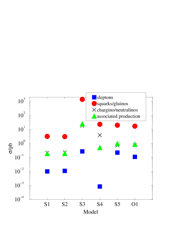
Figure 2: LHC SUSY production hard subprocess total cross sections for the LHC SUGRA points S1-S5 and the optimized string model O1. HERWIG6.0 was used with the CTEQ3L parton distributions. Statistical fractional error on each point is $2\%$. Comparison with SPYTHIA, ISAJET7.40 is shown in Table 2.

Fig. 2 displays the result of the calculation using HERWIG6.0. It is noticeable from the figure that S5 and O1 have broadly similar SUSY production cross-sections except for the sleptons which are noticeably lower. This can be understood by comparing the spectra of the two models, displayed in Table 3. The spectra are approximately similar, except for the sleptons which are heavier in O1 relative to the squarks. This is a consequence of the different choice of modular weights for the sleptons and the squarks. We therefore propose to analyse LHC SUSY production in O1  using S5 as a benchmark or comparison. We will show that the two models can be distinguished experimentally.

$M_{g}$	$m_{u_{L}}$	$m_{u_{R}^{c}}$	$m_{d_{L}}$	$m_{d_{R}^{c}}$	$m_{b_{1}}$	$m_{b_{2}}$	$m_{t_{1}}$	$m_{t_{2}}$	$m_{\nu_{e}}$	$m_{e_{L}}$	$m_{e_{R}^{c}}$	$m_{\nu_{\tau}}$
747	660	632	664	630	608	636	494	670	273	284	217	271
733	654	631	657	628	600	629	460	671	230	239	157	230
$m_{\tau_{1}}$	$m_{\tau_{2}}$	$m_{\chi^{0}_{1}}$	$m_{\chi^{0}_{2}}$	$m_{\chi^{0}_{3}}$	$m_{\chi^{0}_{4}}$	$m_{\chi^{+}_{1}}$	$m_{\chi^{+}_{2}}$	$m_{h^{0}}$	$m_{H^{0}}$	$m_{A^{0}}$	$m_{H^{+}}$
209	285	–125	–234	371	–398	–233	–398	114	450	449	456
157	239	–122	–233	499	–523	–232	–520	94	612	607	612

Table 3: Comparison of sparticle and Higgs spectrum of O1 and S5 (in bold type). These spectra were calculated using ISASUGRA and all masses are quoted in GeV. Sign conventions are as in ISAJET. The masses of the second family of sparticles are approximately equal to those of the first.

3 Experimental observability

3.1 Method

The primary experimental aim is to take previously developed model-independent methods for measuring SUSY particle masses (which were developed at standard SUGRA points) and by testing them in the context of a new optimised model, identify where these methods need to be generalised to perform well in both models. Secondarily it is to be shown that, after modifying these methods’ treatments of the slepton sector, their performance is sufficient to distinguish between the optimised and standard SUGRA scenarios.

Figure 3: “Sequential” decay.

To accomplish these aims, some model-dependent assumptions have to be made. In this analysis, R-parity is taken to be conserved and certain sparticle decay chains are assumed to exist. In R-parity conserving (RPC) models, SUSY particles are only produced in pairs, and the lightest SUSY particle (LSP) is stable. SUSY events contain two of these LSPs which, being only weakly interacting, escape detection and lead to SUSY events with large amounts of missing transverse energy – the standard signature for RPC models. The fact that these massive particles go missing from all RPC SUSY events means that in these models it is not usually possible to measure particle masses by reconstructing entire decay chains. Thus, as in [1], endpoints in kinematic variables constructed from SUSY decay chains must instead be examined. Specifically, the “sequential” decay mode ${\tilde{{q}}}_{L}\rightarrow{{\tilde{{\chi}}}^{0}_{2}}q\rightarrow{\tilde{{l}}}_{R}^{\mp}l^{\pm}_{\rm near}q\rightarrow{{\tilde{{\chi}}}^{0}_{1}}l^{\mp}_{\rm far}l^{\pm}_{\rm near}q$ (see Figure 3) and the “branched” decay modes ${\tilde{{q}}}_{L}\rightarrow{{\tilde{{\chi}}}^{0}_{2}}q\rightarrow{{\tilde{{\chi}}}^{0}_{1}}Xq\rightarrow{{\tilde{{\chi}}}^{0}_{1}}l^{\pm}l^{\mp}q$ (see Figure 4) form the starting point for this investigation.

Figure 4: “Branched” decays through the $Z$ and Higgs bosons.

The kinematic edges used in [1] to identify particle masses at S5 contain:

• $l^{+}l^{-}$ edge: This picks out, from the “sequential” decays, the position of the very sharp edge in the dilepton invariant mass spectrum caused by ${{\tilde{{\chi}}}^{0}_{2}}\rightarrow l{\tilde{{l}}}$ followed by ${\tilde{{l}}}\rightarrow l{{\tilde{{\chi}}}^{0}_{1}}$.

• $l^{+}l^{-}q$ edge: In “sequential” decays, the $llq$ invariant mass spectrum contains a linearly vanishing upper edge due to successive two-body decays. Our theoretical model of the $l^{+}l^{-}q$ edge is more model independent than that used in earlier studies as it does do not assume any relation between the sparticle masses, other than the hierarchy $0<m_{{\tilde{{\chi}}}^{0}_{1}}<m_{{\tilde{{l}}}_{R}}<m_{{\tilde{{\chi}}}^{0}_{2}}<m_{\tilde{{q}}}$ necessary for the “seqential” decay chain to exist at all.

• $l^{+}l^{-}q$ threshold: This is the non-zero minimum in the “sequential” $llq$ invariant mass spectrum, for the subset of events in which the angle between the two leptons (in the centre of mass frame of the slepton) is greater than $\pi/2$. This translates into the direct cut on $m_{ll}$ described in Section 3.4.1.

• $hq$ edge: This is one of the two instances of the $Xq$ edge. In general, the $Xq$ edge is the upper edge of the distribution of the invariant mass of three visible particles in the “branched” decays of Figure 4. The position of this edge is again determined by two-body kinematics. Depending on the Higgs mass and the mass difference between the ${{\tilde{{\chi}}}^{0}_{2}}$ and the ${{\tilde{{\chi}}}^{0}_{1}}$, one of the two “branched” decay chains will be strongly suppressed with respect to the other, so typically only one edge will be visible. At S5 the Higgs mode dominates, while the $Z$ mode will dominate at O1.

As detailed later in this analysis, new edges are added to the list above. Two of them are more general versions of other edges treated in [1], while another is entirely new. They are the ${l^{\pm}q}$ high-, ${l^{\pm}q}$ low- and $M_{T2}$ edges respectively. To summarise, the overall method we apply in this paper consists of:

• finding a model-independent set of cuts which can be used to select events from which the endpoints of all the kinematic edges may be measured,

• obtaining an estimate of the accuracy with which the edge positions might be determined by an LHC experiment,

• performing chi-squared fits of the expected positions of these edges (as functions of the sparticle masses) to a set of “simulated edge measurements” one might expect from an ensemble of such experiments, and

• interpreting the results as the statistics contribution to model independent sparticle mass measurements of a typical LHC experiment.

Were all squarks to have the same mass, then (with perfect detector resolution and with infinite statistics) the endpoints of the edges listed above would be found at the positions given in Table 4. Note that these positions depend on four unknown parameters, namely the masses of the squark, the slepton and the two neutralinos participating in each decay. The mass of the lightest Higgs boson also appears, but we assume this will already be known or will be obtained by other methods (e.g. [26]) to within 2%.

In a more realistic “non-degenerate squark masses” scenario, every distribution with a squark related edge will actually be a superposition of many underlying distributions (one for each squark mass), each having its edge at a slightly different location. This results in some smearing of the edges, even before detector effects (resolutions, acceptances, jet energy calibrations etc.) are taken into account.

Related edge	Kinematic endpoint
$l^{+}l^{-}$ edge	$(m_{ll}^{{\rm max}})^{2}$	$=$	$({\tilde{\xi}}-{\tilde{l}})({\tilde{l}}-{\tilde{\chi}})/{\tilde{l}}$
$l^{+}l^{-}q$ edge	$(m_{llq}^{{\rm max}})^{2}$	$=$	$\left\{\begin{minipage}{252.94499pt} \par\par$\max{\left[{\frac{({\tilde{q}}-{\tilde{\xi}})({\tilde{\xi}}-{\tilde{\chi}})}{{\tilde{\xi}}},\frac{({\tilde{q}}-{\tilde{l}})({\tilde{l}}-{\tilde{\chi}})}{{\tilde{l}}},\frac{({\tilde{q}}{\tilde{l}}-{\tilde{\xi}}{\tilde{\chi}})({\tilde{\xi}}-{\tilde{l}})}{{\tilde{\xi}}{\tilde{l}}}}\right]}$ \par\par except for the special case in which ${\tilde{l}}^{2}<{\tilde{q}}{\tilde{\chi}}<{\tilde{\xi}}^{2}$ and ${\tilde{\xi}}^{2}{\tilde{\chi}}<{\tilde{q}}{\tilde{l}}^{2}$ where one must use $(m_{\tilde{{q}}}-m_{{\tilde{{\chi}}}^{0}_{1}})^{2}$. \par\end{minipage}\right.$
$Xq$ edge	$(m_{Xq}^{{\rm max}})^{2}$	$=$	${X}+({\tilde{q}}-{\tilde{\xi}})\left[{\tilde{\xi}}+{X}-{\tilde{\chi}}+\sqrt{({\tilde{\xi}}-{X}-{\tilde{\chi}})^{2}-4{X}{\tilde{\chi}}}\right]/(2{\tilde{\xi}})$
$l^{+}l^{-}q$ threshold	$(m_{llq}^{{\rm min}})^{2}$	$=$	$\left\{\begin{minipage}{252.94499pt} \par$[\ \ 2{\tilde{l}}({\tilde{q}}-{\tilde{\xi}})({\tilde{\xi}}-{\tilde{\chi}})+({\tilde{q}}+{\tilde{\xi}})({\tilde{\xi}}-{\tilde{l}})({\tilde{l}}-{\tilde{\chi}})$ \par\par$\ \ -({\tilde{q}}-{\tilde{\xi}})\sqrt{({\tilde{\xi}}+{\tilde{l}})^{2}({\tilde{l}}+{\tilde{\chi}})^{2}-16{\tilde{\xi}}{\tilde{l}}^{2}{\tilde{\chi}}}\ \ ]/(4{\tilde{l}}{\tilde{\xi}})$ \par\end{minipage}\right.$
$l^{\pm}_{\rm near}q$ edge	$(m_{l_{\rm near}q}^{{\rm max}})^{2}$	$=$	$({\tilde{q}}-{\tilde{\xi}})({\tilde{\xi}}-{\tilde{l}})/{\tilde{\xi}}$
$l^{\pm}_{\rm far}q$ edge	$(m_{l_{\rm far}q}^{{\rm max}})^{2}$	$=$	$({\tilde{q}}-{\tilde{\xi}})({\tilde{l}}-{\tilde{\chi}})/{\tilde{l}}$
${l^{\pm}q}$ high-edge	$(m_{lq{\rm(high)}}^{{\rm max}})^{2}$	$=$	$\max{\left[{(m_{l_{\rm near}q}^{{\rm max}})^{2},(m_{l_{\rm far}q}^{{\rm max}})^{2}}\right]}$
${l^{\pm}q}$ low-edge	$(m_{lq{\rm(low)}}^{{\rm max}})^{2}$	$=$	$\min{\left[{(m_{l_{\rm near}q}^{{\rm max}})^{2},({\tilde{q}}-{\tilde{\xi}})({\tilde{l}}-{\tilde{\chi}})/(2{\tilde{l}}-{\tilde{\chi}})}\right]}$
$M_{T2}$ edge	$\Delta M$	$=$	$m_{\tilde{{l}}}-m_{{\tilde{{\chi}}}^{0}_{1}}$

Table 4: The absolute kinematic endpoints of invariant mass quantities formed from decay chains of the types mentioned in the text for known particle masses. The following shorthand notation has been used: ${\tilde{\chi}}=m^{2}_{{\tilde{{\chi}}}^{0}_{1}},{\tilde{l}}=m^{2}_{{\tilde{{l}}}_{R}},{\tilde{\xi}}=m^{2}_{{\tilde{{\chi}}}^{0}_{2}},{\tilde{q}}=m^{2}_{\tilde{{q}}}$ and ${X}$ is $m^{2}_{h}$ or $m^{2}_{Z}$ depending on which particle participates in the “branched” decay.

It is not possible to measure each of the squark masses separately. Consequently the quantity $m_{\tilde{{q}}}$ in Table 4 will, after being obtained from the “smeared” edges, represent a squark mass scale rather than a specific squark mass. In all squark related edges, except the $l^{+}l^{-}q$ threshold, the contribution to the outermost part of each edge is provided by the heaviest squarks. In the case of the $l^{+}l^{-}q$ threshold, the “true” endpoint is set by the lightest squark. However, if (as at O1 and S5) the other eleven squarks are much heavier (see Table 3), it is easier to measure the contribution coming from them. A strong correlation between $m_{\tilde{{q}}}$ and the mass of the heaviest squark would therefore be expected.

More work would be required to fully understand the “theoretical” systematic errors including the use of a full simulation of the expected edge positions. Better edge models than those used later in this analysis will definitely be needed to permit measurements of edge positions to be better correlated with functions of the particle masses. Other sources of systematic errors which require further analysis are the detector effects mentioned above, combinatorial backgrounds near the edges and possible cut biases. Such systematic errors can only meaningfully be studied when real data are available.

Although they are beyond the scope of this paper, it is assumed that the above investigations could be performed so as to leave the eventual edge resolutions determined only by statistics and detector resolution. In this analysis, then, all edges are fitted with simple shapes (see Section 7) with the intention of extracting only an estimate of the uncertainty on the edge position, and not to obtain the edge position itself.

The first four edges listed in Table 4 thus constitute a minimal constraint on the four unknown sparticle mass parameters, which may then be further constrained by the other measurements which follow.

3.2 Other measurements

3.2.1 Near, far, high and low ${l^{\pm}q}$ edges

In “sequential” decays there are three observable outgoing particles. There are only four different ways of grouping these particles together, and so only four different invariant masses may be formed from them: $m_{ll}$, $m_{llq}$, $m_{l_{\rm near}q}$ and $m_{l_{\rm far}q}$. The first two of these, $m_{ll}$ and $m_{llq}$, may be formed from the observed momenta without knowledge of which lepton was $l_{\rm near}$ and which was $l_{\rm far}$; only the total lepton four-momentum is required. Edges in these invariant mass distributions have already been described. If it were possible to tag the near- and far- leptons separately, the third and fourth invariant mass combinations could also be formed unambiguously, allowing the positions of two more edges, $m_{l_{\rm near}q}^{{\rm max}}$ and $m_{l_{\rm far}q}^{{\rm max}}$, to play a part in the final fit. However, such tagging is impossible. If further information is to be gathered from these decays in a model independent way, it is then necessary to look for edges in variables (functions of $m_{l_{\rm near}q}$ and $m_{l_{\rm far}q}$) which are observable. On an event-by-event basis, then, we define

$${m_{lq{\rm(high)}}}=\max{({m_{{l^{+}}q},m_{{l^{-}}q}})}\equiv\max{({m_{l_{\rm near}q},m_{l_{\rm far}q}})}$$ (13)

and

$${m_{lq{\rm(low)}}}=\min{({m_{{l^{+}}q},m_{{l^{-}}q}})}\equiv\min{({m_{l_{\rm near}q},m_{l_{\rm far}q}})}.$$ (14)

The simplest theoretical predictions for the positions of the corresponding edges, $m_{lq{\rm(high)}}^{{\rm max}}$ and $m_{lq{\rm(low)}}^{{\rm max}}$, are listed in Table 4, along with the positions of the near- and far-edges. Note that although the position of the high-edge is just the higher of $m_{l_{\rm near}q}^{{\rm max}}$ and $m_{l_{\rm far}q}^{{\rm max}}$, the position of the low-edge has a more interesting form. This asymmetry arises because it is not always kinematically possible for the invariant mass of the lepton/quark pair coming from the lower near/far distribution to approach $\min{\left[{m_{l_{\rm near}q}^{{\rm max}},m_{l_{\rm far}q}^{{\rm max}}}\right]}$ arbitrarily closely, while simultaneously requiring that this invariant mass is less than that of the other lepton/quark pair.

3.2.2 $Zq$ edge

Since the neutralino mass difference at O1 ($109\ {{\rm GeV}}$) is too small to permit ${{\tilde{{\chi}}}^{0}_{2}}\rightarrow h{{\tilde{{\chi}}}^{0}_{1}}$, “branched” decays are mediated by the $Z$. (Particle masses may be seen in Table 3.) The cuts developed in [1] for picking out this special case of the $Xq$ edge at S2 are found to perform equally well at O1, so they are adopted unchanged. Although it might be possible to benefit from adapting these cuts to O1 slightly, this temptation is resisted in order to retain model independence.

3.2.3 $M_{T2}$

In order to constrain the slepton and neutralino masses better, we construct another variable, $M_{T2}(\chi)$, whose distribution relates just these two masses. We base this on the variable, proposed in [2], which looks at events containing two identical two body decays: $xy\rightarrow X\rightarrow Ya_{1}a_{2}\rightarrow Yb_{1}c_{1}b_{2}c_{2}$, where the particles of types $a$ and $c$ are of unknown mass, where particles of type $c$ are undetectable, where the longitudinal momentum of the incoming particles is also unknown, and where it is assumed that $Y$ does not contain any unobservable particles such as neutrinos. In such cases, the variable provides a kinematic constraint on the masses of $a$ and $c$. We seek to apply this primarily to LHC dislepton events of the form $q\bar{q}\rightarrow{\tilde{{l}}}_{R}^{+}{\tilde{{l}}}_{R}^{-}\rightarrow l^{+}{{\tilde{{\chi}}}^{0}_{1}}l^{-}{{\tilde{{\chi}}}^{0}_{1}}$ and so define our $M_{T2}(\chi)$ by:

$${M_{T2}^{2}(\chi)}\equiv{\min_{{{\hbox to0.0pt{\hbox to3.8889pt{\hfil/\hfil}\hss}{\bf p}}}_{1}+{{\hbox to0.0pt{\hbox to3.8889pt{\hfil/\hfil}\hss}{\bf p}}}_{2}={{\hbox to0.0pt{\hbox to3.8889pt{\hfil/\hfil}\hss}{\bf p}}}_{T}}{\Bigl{[}\max{\{m_{T}^{2}({{\bf p}_{T}^{l_{1}}},{{\hbox to0.0pt{\hbox to5.55557pt{\hfil/\hfil}\hss}{\bf p}}}_{1},\chi),m_{T}^{2}({{\bf p}_{T}^{l_{2}}},{{\hbox to0.0pt{\hbox to5.55557pt{\hfil/\hfil}\hss}{\bf p}}}_{2},\chi)\}}\Bigr{]}}}$$ (15)

where

$$m_{T}^{2}({{\bf p}_{T}^{l}},{\bf q}_{T},\chi)\equiv{m_{l}^{2}+\chi^{2}+2(E_{T}^{l}E_{T}^{\chi}-{{\bf p}_{T}^{l}}\cdot{\bf q}_{T})},$$ (16)

$${E_{T}^{l}}={\sqrt{{{\bf p}_{T}^{l}}^{2}+m_{l}^{2}}}\qquad\hbox{and}\qquad{E_{T}^{\chi}}={\sqrt{{\bf q}_{T}^{2}+\chi^{2}}}.$$ (17)

This definition includes the lepton masses for completeness, although these are neglected in all computations.

The value $M_{T2}(\chi)$ takes for a given candidate dislepton event is a function of: the transverse missing-momentum vector, ${{\hbox to0.0pt{\hbox to5.55557pt{\hfil/\hfil}\hss}{\bf p}}}_{T}$; the transverse momentum vectors of the two leptons, ${{\bf p}_{T}^{l_{1}}}$ and ${{\bf p}_{T}^{l_{2}}}$; and one other parameter – an estimate of the neutralino mass, $\chi$ (not to be confused with the actual mass of the neutralino, $m_{{\tilde{{\chi}}}^{0}_{1}}$). Unlike the other parameters, the value of $\chi$ is not measured in each event – events may be reinterpreted for different values of $\chi$. $M_{T2}(\chi)$ has the property that, for signal events in a perfect detector,

$${\max_{\rm events}{\left[{M_{T2}(m_{{\tilde{{\chi}}}^{0}_{1}})}\right]}}=m_{{\tilde{{l}}}}.$$ (18)

Thus when $\chi$ is indeed $m_{{\tilde{{\chi}}}^{0}_{1}}$, then the distribution of $M_{T2}$ has an end point at the slepton mass. Since the other observables allow $m_{{\tilde{{\chi}}}^{0}_{1}}$ to be measured in a model independent way, $M_{T2}$ can then be included in the analysis to provide an additional constraint on the slepton/neutralino mass difference.

In practice the $M_{T2}$ edge can be distorted by the finite resolution of the detector or missing energy from soft underlying events. Additionally, standard model (SM) backgrounds provide constraints on minimum detectable slepton/neutralino mass differences (see Section 10). However the most important factor to control is the ability to correctly identify which particle species is contributing to an observed $M_{T2}$ edge – particularly since it is possible to have multiple edges in the non standard model contributions to $M_{T2}$ distributions. At S5, for example, where both the right- and left-sleptons are lighter than at O1 (see Table 3), both ${\tilde{{l}}}_{R}^{+}{\tilde{{l}}}_{R}^{-}$ and ${\tilde{{l}}}_{L}^{+}{\tilde{{l}}}_{L}^{-}$ events pass the cuts, and two edges are generated. The edge coming from the (lighter) right-slepton falls well under the SM background and so is not measurable, while the (heavier) left-slepton still has a cross section for pair-production high enough to let it form a good edge of its own at $M_{T2}({m_{{\tilde{{\chi}}}^{0}_{1}}})=m_{{\tilde{{l}}}_{L}}$. It is important that this edge is not mistaken for the ${\tilde{{l}}}_{R}$, so methods are needed to dismiss it. A detailed prescription of how to go about such a dismissal is beyond the scope of this paper, but it would clearly be accomplished by looking for inconsistency between a given edge-particle hypothesis and all the other sparticle masses, the branching ratios and (in particular) the strongly mass dependent pair-production cross sections, which could all be measured by other means.

3.3 Event generation and detector simulation

All events, except those from $q\bar{q}\rightarrow W^{+}W^{-}$ background processes, are simulated by HERWIG6.0. The $W$-pair events are generated by ISAJET7.42 [22]. The detector chosen for simulation is the ATLAS detector [27, 28, 29], one of the two general purpose experiments scheduled for the LHC. The LHC is expected to start running at a luminosity of about $10^{33}\ {\rm cm}^{-2}{\rm s}^{-1}$ and this is expected to be increased over a period of about three years to the design luminosity of $10^{34}\ {\rm cm}^{-2}{\rm s}^{-1}$. These two periods are referred to, respectively, as the periods of low and high luminosity running.

The performance of the detector is simulated by ATLFAST2.16 [30] which is primarily a fast calorimeter simulation which parametrises detector resolution and energy smearing and identifies jets and isolated leptons, in both the low and high luminosity environments. Throughout this analysis, the parameters controlling ATLFAST’s jet and lepton isolation criteria are left with the default values appropriate to the apparatus: i.e. jets must satisfy ${p_{T}^{j}}\geq 15\ {{\rm GeV}}$ and must lie in the pseudo-rapidity range $-5\leq{\eta^{j}}\leq 5$, while electrons must have ${p_{T}^{l}}\geq 5\ {{\rm GeV}}$, muons ${p_{T}^{l}}\geq 6\ {{\rm GeV}}$ and both must lie in $-2.5\leq{\eta^{l}}\leq 2.5$. For lepton isolation a maximum energy of $10\ {{\rm GeV}}$ may be deposited in a cone about the lepton of radius 0.2 in $(\eta,\phi)$-space ($\phi$ being the azimuthal angle) while its separation from other jets must be at least 0.4 in the same units.

At high luminosity approximately 20 minimum bias events (“pile-up” events) are expected to occur in each bunch crossing. Pile-up events are not simulated by ATLFAST2.16, although it does alter its reconstruction resolutions to reflect the two different luminosity environments. It must be checked that any cuts applied at high luminosity will not be affected substantially by pile-up events. Within this article, events corresponding to $100\ {{\rm fb}^{-1}}$ are generated and are reconstructed in the high luminosity environment. This approximately corresponds to one year of high luminosity running.

3.4 Event selection cuts

Section 3.4.1 summarises all the cuts used to obtain the edges. The $l^{+}l^{-}$ edge, $l^{+}l^{-}q$ edge and $l^{+}l^{-}q$ threshold cuts do not differ significantly from those used in [1]. The ${l^{\pm}q}$ edge cuts, however, do. The most significant change is the relaxation of the splitting requirement. The original splitting requirement tries to guarantee that the jet which comes from the quark produced in association with the observed dilepton pair is correctly identified. It achieves this by insisting that:

• both the dilepton pair and one of the two hardest jets $j_{1}$ and $j_{2}$ (ranked by ${p_{T}}$) are consistent with being the decay products of a squark (i.e. $m_{ll{j_{i}}}<{m_{\rm cutoff}}$), and

• the invariant mass $m_{ll{j_{j}}}$ of the two leptons and the other of the two highest ${p_{T}}$ jets is inconsistent with these being the decay products of a squark (i.e. $m_{ll{j_{j}}}>{m_{\rm cutoff}}$).

Although the above demand for inconsistency increases the purity of the signal, it has a significant detrimental effect on the efficiency. In our analysis the consistency requirement is retained but the inconsistency requirement dropped. Instead we require that $m_{ll}$ is inside the expected region, given the $l^{+}l^{-}$ edge measurement. We also perform background subtraction, modelling the opposite-sign same-lepton-family (OSSF) backgrounds by the distributions produced by those opposite-sign different-lepton-family (OSDF) events which pass the same cuts.

The production cross section for dislepton events suitable for $M_{T2}$ analysis is, in all models, by far the smallest (see Figure 2). So to show that $M_{T2}$ events passing cuts are not in danger of being swamped by small variations in backgrounds or the cuts themselves, two set of cuts referred to as “hard” and “soft” are developed. The “hard” cuts attempt to maximise the signal to background ratio in the vicinity of the dislepton edge in the $M_{T2}$ spectrum, while the much looser “soft” cuts try to maximise statistics at the edge at the expense of allowing in additional SUSY backgrounds.

3.4.1 Cuts listed by observable

This section summarises the cuts used in the analysis. For notational purposes, reconstructed leptons and jets are sorted by ${p_{T}}$. For example $j_{2}$, with corresponding transverse momentum ${\bf p}^{j_{2}}_{T}$, is the reconstructed jet with the second highest ${p_{T}}$. All cuts are requirements unless stated otherwise.

$l^{+}l^{-}$ edge

${n_{\rm leptons}}=2$, both leptons OSSF and ${p_{T}^{l_{1}}}\geq{p_{T}^{l_{2}}}\geq 10\ {{\rm GeV}}$.

${n_{\rm jets}}\geq 2$ and ${p_{T}^{j_{1}}}\geq{p_{T}^{j_{2}}}\geq 150\ {{\rm GeV}}$. $\hbox to0.0pt{\hbox to5.03125pt{\hfil/\hfil}\hss}p_{T}\geq 300\ {{\rm GeV}}$.

The kinematics of OSSF leptons coming from background processes which produce uncorrelated leptons (for example tau decays) are modelled well by OSDF lepton combinations. Consequently, edge resolution is improved by “flavour subtracting” OSDF event distributions from OSSF event distributions.

$l^{+}l^{-}q$ edge

${n_{\rm leptons}}=2$, both leptons OSSF and ${p_{T}^{l_{1}}}\geq{p_{T}^{l_{2}}}\geq 10\ {{\rm GeV}}$.

${n_{\rm jets}}\geq 4$, ${p_{T}^{j_{1}}}\geq 100\ {{\rm GeV}}$, and ${p_{T}^{j_{1}}}\geq{p_{T}^{j_{2}}}\geq{p_{T}^{j_{3}}}\geq{p_{T}^{j_{4}}}\geq 50\ {{\rm GeV}}$.

$\hbox to0.0pt{\hbox to5.03125pt{\hfil/\hfil}\hss}p_{T}\geq\max{({100\ {{\rm GeV}},0.2{M_{\rm effective}}})}$ and ${M_{\rm effective}}\geq 400\ {{\rm GeV}}$, where ${M_{\rm effective}}$ is defined by the scalar sum:

$${M_{\rm effective}}=\hbox to0.0pt{\hbox to7.95831pt{\hfil/\hfil}\hss}E_{T}+{p_{T}^{j_{1}}}+{p_{T}^{j_{2}}}+{p_{T}^{j_{3}}}+{p_{T}^{j_{4}}}.$$ (19)

Since the desired edge is a maximum, only the smaller of the two $m_{llq}$ combinations which can be formed using $j_{1}$ or $j_{2}$ is used.

Flavour subtraction is employed here as at the $l^{+}l^{-}$ edge.

$l^{+}l^{-}q$ threshold

All the cuts for the $l^{+}l^{-}$ edge as above.

In addition ${m_{ll}^{{\rm max}}}/\sqrt{2}\leq m_{ll}\leq m_{ll}^{{\rm max}}$, where the value of $m_{ll}^{{\rm max}}$ would be obtained from the $l^{+}l^{-}$ edge in practice, but was determined theoretically in this analysis.

Since the desired edge is a minimum, only the larger of the two $m_{llq}$ combinations which can be formed using $j_{1}$ or $j_{2}$ is used.

$hq$ edge

${n_{\rm leptons}}=0$ and $\hbox to0.0pt{\hbox to5.03125pt{\hfil/\hfil}\hss}p_{T}>300\ {{\rm GeV}}$.

Exactly two $b$ jets with ${p_{T}^{j_{b_{1}}}}\geq{p_{T}^{j_{b_{2}}}}\geq 50\ {{\rm GeV}}$. No other $b$ jets, regardless of ${p_{T}}$.

At least two non-$b$ jets with ${p_{T}^{j_{q_{1}}}}\geq{p_{T}^{j_{q_{2}}}}\geq 100\ {{\rm GeV}}$, with at least one inside $-2.0\leq{\eta^{j}}\leq 2.0$.

$m_{bb}$ within $17\ {{\rm GeV}}$ of Higgs peak in $m_{bb}$ spectrum.

Since the desired edge is a maximum, the non-$b$ jet (i.e. $j_{q_{1}}$ or $j_{q_{2}}$) chosen to form the $m_{hq}$ invariant mass is that which minimises $m_{hq}$.

$Zq$ edge

${n_{\rm leptons}}=2$, both leptons OSSF and ${p_{T}^{l_{1}}}\geq{p_{T}^{l_{2}}}\geq 10\ {{\rm GeV}}$.

$m_{ll}$ within 2.5 GeV of the centre of the Z-mass peak in the $m_{ll}$ spectrum.

At least two non-$b$ jets exist with ${p_{T}^{j}}\geq 100\ {{\rm GeV}}$ and $\hbox to0.0pt{\hbox to5.03125pt{\hfil/\hfil}\hss}p_{T}\geq 300\ {{\rm GeV}}$.

Since the desired edge is a “maximum”, the jet chosen to form the $m_{Zq}$ invariant mass is the one (from those with ${p_{T}^{j}}\geq 100\ {{\rm GeV}}$) which minimises $m_{Zq}$.

Again, flavour subtraction is used.

${l^{\pm}q}$ high and ${l^{\pm}q}$ low edges

All the cuts for the $l^{+}l^{-}q$ edge above are required.

Additionally, events consistent with the $l^{+}l^{-}$ edge measurement are selected by asking for $m_{ll}\leq m_{ll}^{{\rm max}}+1\ {{\rm GeV}}$.

To choose the jet from which to form $m_{{l^{\pm}q}}$ we select $j_{i}=j_{1}$ or $j_{2}$, whichever gives the smaller value of $m_{llj}$, and require $m_{llj_{i}}<{m_{\rm cutoff}}$, where ${m_{\rm cutoff}}$ is chosen to be above the $l^{+}l^{-}q$ edge, but is otherwise arbitrary. For easy comparison with [1], ${m_{\rm cutoff}}=600\ {{\rm GeV}}$ was used in this analysis.

Finally, the two invariant mass combinations, $m_{{l^{\pm}q}}$, are assigned to $m_{lq{\rm(high)}}$ and $m_{lq{\rm(low)}}$ as defined earlier by Equations (13) and (14).

$M_{T2}$ edge (hard cuts)

Events are required to have exactly one OSSF pair of isolated leptons satisfying ${p_{T}^{l_{1}}}>50\ {{\rm GeV}}$ and ${p_{T}^{l_{2}}}>30\ {{\rm GeV}}$.

$\delta_{T}<20\ {{\rm GeV}}$ is required, where ${\bf\delta}_{T}=|{{{\bf p}_{T}^{l_{1}}}+{{\bf p}_{T}^{l_{2}}}+{{\hbox to0.0pt{\hbox to5.55557pt{\hfil/\hfil}\hss}{\bf p}}}_{T}}|$. Large $\delta_{T}$ in signal events is indicative of an unidentifiable transverse boost to the centre of mass frame, perhaps due to initial state radiation. Large $\delta_{T}$ in other (not necessarily signal) events simply suggests an inconsistency with the desired event topology.

Events containing one or more jets with ${p_{T}^{j}}>40\ {\rm to}\ 50\ {{\rm GeV}}$ are vetoed. This cut also helps to reduce standard model backgrounds, notably $t\bar{t}$. The lower this cut is placed, the better for the background rejection. However the cut cannot be placed too low (especially at high luminosity) due to the significant number of jets coming from the underlying event and other minimum bias events in the same bunch crossing. For order 25 minimum bias events per bunch crossing, [31] estimates that about 10% (1%) of bunch crossings will include a jet from the underlying event with a ${p_{T}}$ greater than 40 GeV (50 GeV). Our results are not sensitive to variation of the jet veto cut between 40 and 50 GeV, where at least 90% signal efficiency is expected.

Events with ${|{m_{l_{1}l_{2}}-m_{Z}}|}<5\ {{\rm GeV}}$ are vetoed to exclude lepton pairs from $Z$ bosons.

$m_{l_{1}l_{2}}>80\ {{\rm GeV}}$ and $\hbox to0.0pt{\hbox to5.03125pt{\hfil/\hfil}\hss}p_{T}>80\ {{\rm GeV}}$ are also required.

$M_{T2}$ edge (soft cuts)

These are as above, but

• the $\hbox to0.0pt{\hbox to5.03125pt{\hfil/\hfil}\hss}p_{T}$ requirement is lowered from 80 to 50 GeV,

• the upper limit for $\delta_{T}$ is extended from 20 to 90 GeV, and

• the dilepton invariant mass cut is removed altogether.

3.5 Edge resolutions

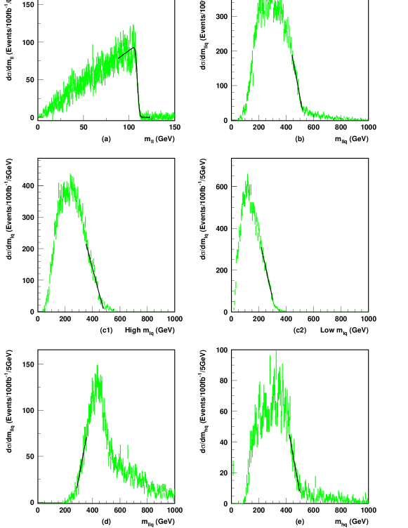
Figure 5: The S5 distributions whose endpoints are described in Table 4: a) the $l^{+}l^{-}$ edge, b) the $l^{+}l^{-}q$ edge, c1) the ${l^{\pm}q}$ high-edge  c2) the ${l^{\pm}q}$ low-edge, d) the $l^{+}l^{-}q$ threshold and e) the $hq$ edge. Plots were produced with the cuts described in Table 3.4.1. The number of events corresponds to $100\ {{\rm fb}^{-1}}$ of high luminosity running.

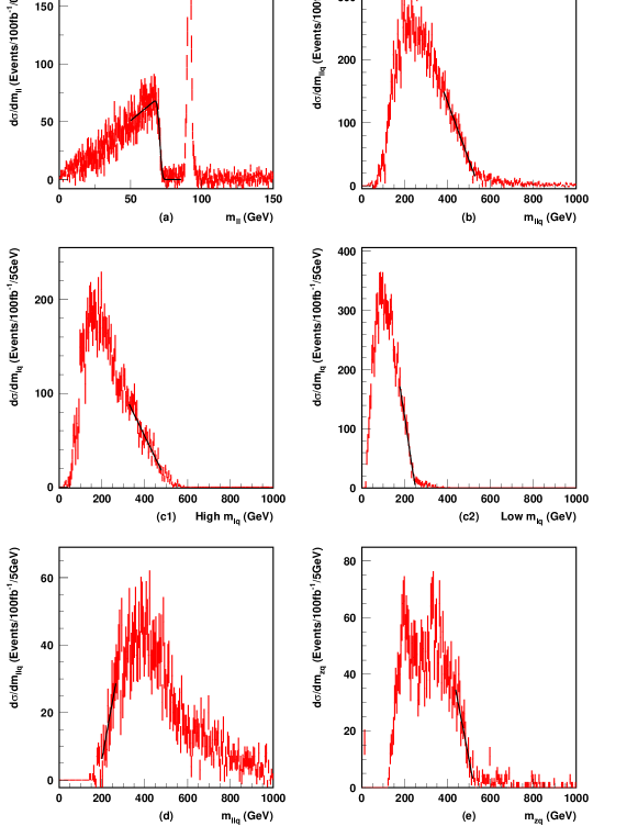
Figure 6: The O1 distributions whose endpoints are described in Table 4: a) the $l^{+}l^{-}$ edge, b) the $l^{+}l^{-}q$ edge, c1) the ${l^{\pm}q}$ high-edge  c2) the ${l^{\pm}q}$ low-edge, d) the $l^{+}l^{-}q$ threshold and e) the $Zq$ edge. Plots were produced with the cuts described in Table 3.4.1. The number of events corresponds to $100\ {{\rm fb}^{-1}}$ of high luminosity running.

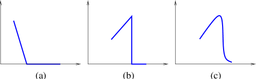
Figure 7: Line-shapes used for fits to the mass distributions. Shape (a) (or its reflection in the vertical axis) is the standard “straight line” used to extract the $l^{+}l^{-}q$ edge, ${l^{\pm}q}$ high-edge, ${l^{\pm}q}$ low-edge and $l^{+}l^{-}q$ threshold resolutions. Shape (b) models the expected shape of the sharp $l^{+}l^{-}$ edge in the absence of detector effects. The $l^{+}l^{-}$ edge is actually fitted with shape (c), which is identical to (b) except that it is smeared with a gaussian resolution whose width is a free parameter of the fit.

By applying at S5 the cuts listed in Section 3.4.1 we reproduce the $m_{ll}$ and $m_{llq}$ distributions whose edges are analyzed in [1] (see Figure 5: a, b and d). We also confirm that the same cuts may also be used to generate edges of similar quality at O1 (see Figure 6: a, b and d). In addition, plots c1 and c2 in Figures 5 and 6 display the $m_{lq{\rm(high)}}$ and $m_{lq{\rm(low)}}$ distributions generated from the modified ${l^{\pm}q}$ edge cuts also listed above. Numerical results are summarised in Table 5.

Similar pictures are seen at S5 and O1. The most obvious difference between the two sets of data is the peak at the $Z$ mass present in Figure 6a but absent in Figure 5a. This peak comes from direct ${{\tilde{{\chi}}}^{0}_{2}}\rightarrow{{\tilde{{\chi}}}^{0}_{1}}Z\rightarrow{{\tilde{{\chi}}}^{0}_{1}}l^{+}l^{-}$ decays, which have a branching fraction of 39% at O1 compared with 0.65% at S5. The most common direct neutralino decay mode at S5 is through the $h_{0}$ ( 65% ) of which only a tiny proportion ( 0.02% ) decay to the two light leptons – the partial decay width $\Gamma({{h_{0}}\rightarrow{ff}})$ going approximately as $m_{f}^{2}$. Scenarios in which the $l^{+}l^{-}$ edge happens to coincide with the $Z$ peak require special treatment and are not considered here.

In order to make useful statements about the degree to which model parameters may be extracted from the endpoints and edges of these distributions, it is necessary to obtain an estimate of the accuracy with which these observables may be measured. It is expected that the errors on all of the observables considered here will eventually be statistics dominated, so simple fits have been made to the data to obtain estimates of the statistical errors on the edge or end point locations. The shapes fitted to the data (see Figure 7) and the algorithms for determining the boundaries of the fitted regions have been kept as simple and generic as possible, with the intention of making the fit results both conservative and simple to interpret. Given real data, it would be worth putting substantial effort into understanding how detector and physics effects affect the shape of each distribution in turn. This could significantly improve particle mass resolutions. The resolutions obtained from the fits to the distributions in Figure 5 and Figure 6 are listed in Table 5.

The $M_{T2}$ distributions obtained after the cuts listed in Section $M_{T2}$ edge (soft cuts) are shown in Figure 8. The signal dislepton region having the desired edge is the unhatched region on each plot. Conveniently, most of the other SUSY events passing the cuts (mainly events containing gauginos) are also distributed with an edge located at a similar position to the disleptons’. This is due to the fact that such events often include pairs of slepton decays, and these may sometimes occur in combination with low jet activity and without additional leptons being produced inside detector acceptance. Consequently, for much of the SUSY background which passes cuts, the cuts are accepting $M_{T2}$ values which do not degrade edge performance significantly. Note that $\Delta M(\chi)={M_{T2}(\chi)}-{\chi}\geq 0$ is plotted evaluated at $\chi=m_{{\tilde{{\chi}}}^{0}_{1}}$, so this should have an edge at $\Delta M_{\rm max}=m_{\tilde{{l}}}-m_{{\tilde{{\chi}}}^{0}_{1}}$. Of course, $m_{{\tilde{{\chi}}}^{0}_{1}}$ is not actually known a priori, so generating this graph in a real experiment requires an estimate of $m_{{\tilde{{\chi}}}^{0}_{1}}$ to be obtained by other means. For our purposes it will be sufficient if the position of the edge of the distribution can be measured to about 10%, and this determines the accuracy required of the neutralino mass estimate $\chi$. The width $\Delta M(\chi)=M_{T2}(\chi)-\chi$ remains approximately stable at the 10% level for $m_{{\tilde{{\chi}}}^{0}_{1}}/2<\chi<2m_{{\tilde{{\chi}}}^{0}_{1}}$. To illustrate the relative insensitivity of $\Delta M_{\rm max}(\chi)$ to $\chi$ near $m_{{\tilde{{\chi}}}^{0}_{1}}$, plots generated from the same data as before but with $\chi\approx m_{{\tilde{{\chi}}}^{0}_{1}}\pm 50\ {{\rm GeV}}$ are shown in Figure 9. Satisfying the 10% requirement above by obtaining a suitable value of $\chi$ within such a $\pm 40\%$ range is not difficult and may be accomplished by first performing a “cut down” version of the analysis described later in the text, but omitting the $M_{T2}$ data, and then choosing the estimate, $\chi$, to be the resulting reconstructed neutralino mass.

Determining the likely resolution for the $M_{T2}$ edge requires a slightly different approach to that used for the other edges. Whereas the cuts used to obtain the invariant mass distributions have high SM rejections (primarily due to the presence of at least one high mass $\hbox to0.0pt{\hbox to5.03125pt{\hfil/\hfil}\hss}p_{T}$ or ${M_{\rm effective}}$ cut), the $M_{T2}$ cuts cannot be so hard, primarily because the desired dislepton events have have very little jet activity. With the dislepton production cross sections typically two orders of magnitude smaller than the squark/gluino production cross sections (Table 2) a low efficiency is not affordable. There are also irreducible SM backgrounds (primarily $W^{+}W^{-}\rightarrow l^{+}l^{-}\nu\bar{\nu}$ but also ${t{\bar{t}}}\rightarrow b\bar{b}W^{+}W^{-}\rightarrow jjl^{+}l^{-}\nu\bar{\nu}$ in cases where jets are below the ${p_{T}}$ cut or outside detector acceptance) which have signatures identical to dislepton events. These backgrounds are clearly visible in Figure 8 and would cause problems for naive straight line fitting techniques.

Figure 8: These $M_{T2}$ distributions for O1 are generated from 100 events ${{\rm fb}^{-1}}$ at high luminosity, and from the $M_{T2}$ cuts described in section 3.4. (a) and (b) use the “hard” cuts, while (c) and (d) use the “soft” cuts. In (a) and (c), events containing a jet with $p_{T}>40\ {{\rm GeV}}$ were vetoed. In (b) and (d), this cut was relaxed to $50\ {{\rm GeV}}$. In all plots, $M_{T2}(\chi)$ is evaluated at $\chi=m_{{\tilde{{\chi}}}^{0}_{1}}$. The results are presented in the form $M_{T2}(m_{{\tilde{{\chi}}}^{0}_{1}})-m_{{\tilde{{\chi}}}^{0}_{1}}$ in order to show the edge of the signal region located at the difference between the slepton and neutralino masses (92.5 GeV).

Figure 9: These two plots are identical to Figure 8(d) except that the true neutralino mass (125 GeV) is not presupposed. Instead, (a) uses $\chi=70\ {{\rm GeV}}$ and (b) uses $\chi=170\ {{\rm GeV}}$.

Figure 10: Variation with $\chi$ of the SM contributions to $\max(M_{T2}(\chi)-\chi)$ (for a number of events corresponding to $100\ {{\rm fb}^{-1}}$) which provides a measure of the minimum ${\tilde{{l}}}$-${{\tilde{{\chi}}}^{0}_{1}}$ mass difference which is needed for signal $M_{T2}$ events to be able to extend beyond the SM backgrounds. Events contributing to this plot were selected using the “hard” $M_{T2}$ cuts.

The standard model backgrounds in Figure 8, although large, are easy to control. The SM edge is very clean, since the events which pass the cuts are well reconstructed and there are no noticeable tails. The SM edge will fall at $m_{W}$ for $\chi=0$, corresponding to the mass of the missing neutrino in SM events. As $\chi$ increases, the SM edge recedes to lower masses as shown in Figure 10, falling to $60\ {{\rm GeV}}$ for $\chi=100\ {{\rm GeV}}$. A significant excess of events above this threshold would be a clear signal for non-SM processes. Such an excess will appear when the ${\tilde{{l}}}$-${{\tilde{{\chi}}}^{0}_{1}}$ mass difference exceeds $80\ {{\rm GeV}}$ for low $m_{{\tilde{{\chi}}}^{0}_{1}}$ and $50\ {{\rm GeV}}$ for high $m_{{\tilde{{\chi}}}^{0}_{1}}$.

We estimate that, using $M_{T2}$ with either set of cuts, it is possible to measure $\Delta M_{\rm max}=m_{\tilde{{l}}}-m_{{\tilde{{\chi}}}^{0}_{1}}$ to 10% or better. The “hard” $M_{T2}$ cuts successfully remove almost all SUSY background above the SM threshold at the expense of only retaining half of the events passing the “soft” cuts. For both sets of cuts the SM threshold, at about 60 GeV, would be approximately three sigma away from $\Delta M_{\rm max}$ at this accuracy.

	S5		O1		Table 4 values
Endpoint	Fit	Fit error	Fit	Fit error	S5	O1
$l^{+}l^{-}$ edge	109.10	0.13	70.47	0.15	109.12	70.50
$l^{+}l^{-}q$ edge	532.1	3.2	544.1	4.0	536.7	530.5
${l^{\pm}q}$ high-edge	483.5	1.8	515.8	7.0	464.2	513.6
${l^{\pm}q}$ low-edge	321.5	2.3	249.8	1.5	337.0	231.3
$l^{+}l^{-}q$ threshold	266.0	6.4	182.2	13.5	264.9	168.1
$Xq$ edge	514.1	6.6	525.5	4.8	509.2	503.4
$\Delta M$ ($M_{T2}$ edge)	——	——	——	10%	35.7	92.5

Table 5: Endpoints and associated fit uncertainties. The results of the naive fits shown in Figures 5 and 6 may be seen in the ‘fit’ and (one-sigma) ‘fit error’ columns. For the reasons outlined in Section 4 there is presently a lack of good theoretical predictions for these edge positions. (In this context a “good prediction” is one capable of taking into account, up to a level compatible with the statistical/fit errors, either the naivety of the fits, or the effects introduced by edge distortions and the presence of backgrounds.) The best guides presently available are the quantities listed in Table 4, evaluated at $m_{\tilde{{q}}}$ equal to the largest squark mass. These values are also shown for comparison purposes. All values are GeV except where stated otherwise.

3.6 Reconstructing sparticle masses

Sparticle masses are reconstructed by performing a chi-squared fit with between four and six free parameters $p$. The main parameters of the fit are $m_{{\tilde{{\chi}}}^{0}_{1}}$, $m_{\tilde{{l}}}$, $m_{{\tilde{{\chi}}}^{0}_{2}}$ and $m_{\tilde{{q}}}$. Where appropriate, $m_{h}$ and $m_{Z}$ also appear as fit parameters, although if they do, they are strongly constrained (particularly in the case of the $Z$) by present LEP measurements or expected LHC errors (0.0077% and 2.0% respectively).

The chi-squared, as a function of the free parameters $p$, is then formulated as:

$$\chi^{2}{(p)}=\sum^{n}_{1}{\frac{{({O^{\rm sm}_{i}-O_{i}(p)})}^{2}}{{\sigma_{i}}^{2}}},$$ (20)

where $O^{\rm sm}_{i}=O_{i}({p_{\rm model}})+\sigma_{i}X_{i}$ are $n$ “smeared observables”, $X_{i}\sim N({0,1})$ are the $n$ random variables from the Normal distribution (with mean 0 and standard deviation 1) which accomplish the smearing, $\sigma_{i}$ is the anticipated statistical error for the $i^{\rm th}$ observable (approximated by the fit error listed in Table 5), and $O_{i}(p)$ is the value one would expect for the $i^{\rm th}$ observable given the parameters $p$ (for examples see Table 4). $p_{\rm model}$ indicates the actual masses of the sparticles in the particular model being considered. The results of the fit, $p_{\rm fit}$, are then those which minimise the chi-squared. $p_{\rm fit}$ may be interpreted as the sparticle masses which might be reconstructed by an LHC experiment after obtaining $100{{\rm fb}^{-1}}$ at high luminosity, with the $X_{i}$ parametrising the experimental errors. In order to determine the accuracy with which this reconstruction can be performed, the above fitting process is repeated many times for different values of the $X_{i}$, producing the distributions of reconstructed particle masses which follow.

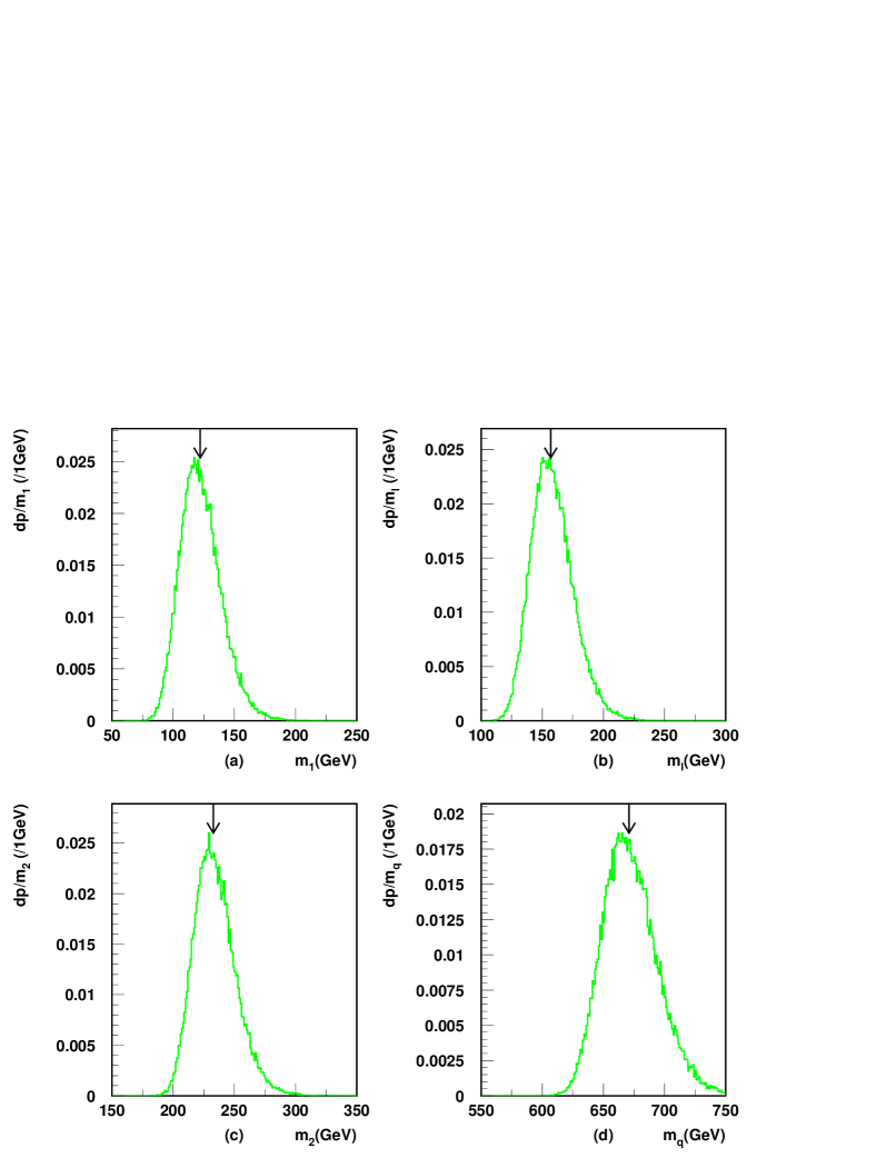
Figure 11: Reconstructed ${{\tilde{{\chi}}}^{0}_{1}}$, ${\tilde{{l}}}$, ${{\tilde{{\chi}}}^{0}_{2}}$ and ${\tilde{{q}}}$ masses at S5. The small arrows indicate the masses used as the input parameters, $p_{\rm model}$.

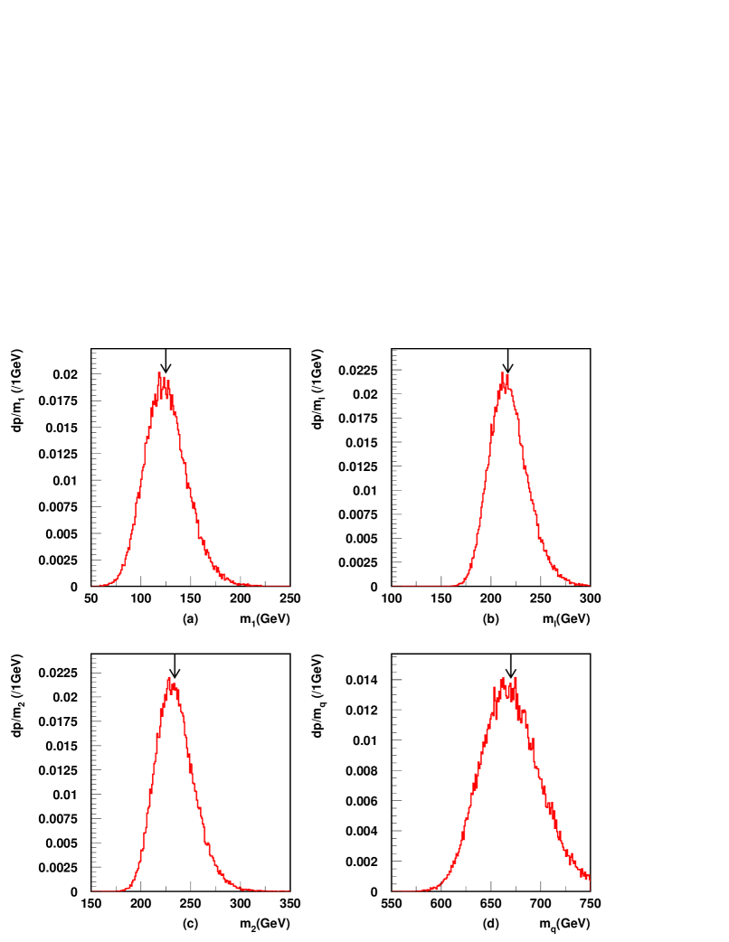
Figure 12: Reconstructed ${{\tilde{{\chi}}}^{0}_{1}}$, ${\tilde{{l}}}$, ${{\tilde{{\chi}}}^{0}_{2}}$ and ${\tilde{{q}}}$ masses at O1. The small arrows indicate the masses used as the input parameters, $p_{\rm model}$.

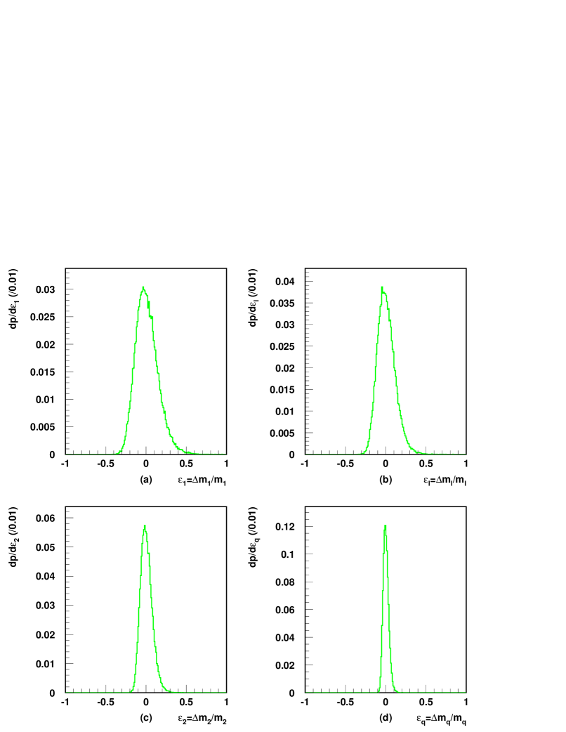
Figure 13: Fractional errors in reconstructed ${{\tilde{{\chi}}}^{0}_{1}}$, ${\tilde{{l}}}$, ${{\tilde{{\chi}}}^{0}_{2}}$ and ${\tilde{{q}}}$ masses at S5.

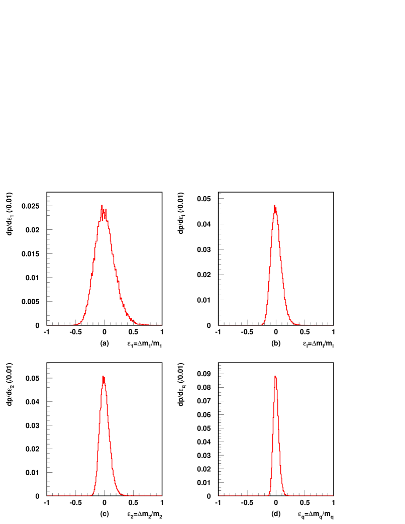
Figure 14: Fractional errors in reconstructed ${{\tilde{{\chi}}}^{0}_{1}}$, ${\tilde{{l}}}$, ${{\tilde{{\chi}}}^{0}_{2}}$ and ${\tilde{{q}}}$ masses at O1.

	Fractional RMS		Fractional mean		Reconstruction width
	$\sqrt{\overline{\varepsilon^{2}_{p}}}$		$\overline{\varepsilon_{p}}/{{10}^{-3}}$		$\sqrt{\overline{(m_{p}-\overline{m_{p}})^{2}}}$
$p$	S5	O1	S5	O1	S5	O1
${{\tilde{{\chi}}}^{0}_{1}}$	0.140	0.175	11.4	8.0	$17\ {{\rm GeV}}$	$22\ {{\rm GeV}}$
${\tilde{{l}}}_{R}$	0.112	0.091	8.8	5.7	$17\ {{\rm GeV}}$	$20\ {{\rm GeV}}$
${{\tilde{{\chi}}}^{0}_{2}}$	0.074	0.084	6.0	5.3	$17\ {{\rm GeV}}$	$20\ {{\rm GeV}}$
${\tilde{{q}}}$	0.034	0.047	2.7	2.4	$22\ {{\rm GeV}}$	$29\ {{\rm GeV}}$

Table 6: RMS and mean values, for each of the particles $p$, of the fractional mass-error distributions ($\varepsilon_{p}$) in Figures 13 and 14. Also shown are the widths of the distributions of the reconstructed particle masses (from Figures 11 and 12).

Figures 11 and 12 show the probability distributions expected for the reconstructed ${{\tilde{{\chi}}}^{0}_{1}}$, ${\tilde{{l}}}$, ${{\tilde{{\chi}}}^{0}_{2}}$ and ${\tilde{{q}}}$ masses, while Figures 13 and 14 show the corresponding fractional errors, $\varepsilon_{p}$, for the same quantities. All are approximately Gaussian and have reassuringly small tails. Statistics summarising these plots (widths, means and RMS values) are listed in Table 6.

It may be seen that in both O1 and S5 the widths of the mass distributions for all four particles are very similar. This is because, in localized regions of parameter space, the edges tend to constrain mass differences far better than absolute masses. Evidence of this may be seen in Figure 15 which shows the scatter of reconstructions in the $m_{{\tilde{{\chi}}}^{0}_{1}}$-$m_{{\tilde{{l}}}_{R}}$ plane. It is interesting to note that without the $M_{T2}$ constraint at O1, the fit’s chi-squared commonly has two distinct and competing comparable minima – one at high and one at low values of $m_{{\tilde{{l}}}_{R}}$. The simultaneous existence of these minima is a direct consequence of putting the near and far ${l^{\pm}q}$ edges on an equal footing in this analysis, allowing more than one interpretation for each of the high and low edges. The need to resolve this kind of ambiguity in model-independent investigations of this type illustrates the importance of establishing reliable model-independent ways of measuring the absolute scale of $m_{{\tilde{{l}}}_{R}}-m_{{\tilde{{\chi}}}^{0}_{1}}$ (or a related quantity) even if only to an accuracy of 20-30%.

The clear gap between the reconstruction regions for O1 and S5 in Figure 15 supports the original claim that, systematic errors permitting, it will be possible to distinguish between the two scenarios.

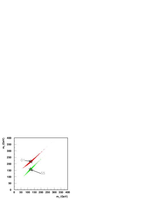
Figure 15: Reconstructed $m_{\tilde{{l}}}$ versus $m_{{\tilde{{\chi}}}^{0}_{1}}$ for ${O1}$ and ${S5}$. The stars show the true masses for each model.

4 Conclusions

Some of the five standard LHC SUGRA points are compatible with universal perturbative string and M-theory, but dangerous CCB/UFB breaking minima are present in each example. We therefore studied a perturbative string model which is optimized to ameliorate the CCB/UFB problems present in the other models. The optimized model is non-universal because the squarks and sleptons are split in mass at the string scale. We identify the SUGRA point with the most similar spectrum and hard SUSY production cross sections (S5) to compare the optimized model with. The main difference is that the sleptons are heavier and therefore have lower production cross-sections. We have demonstrated the existence of a method by which an LHC experiment will be able to measure the masses of the (lighter) sleptons and the two neutralinos at O1 in a largely model independent way. In a specific comparison of S5 and O1 we have shown that this method will be able to distinguish a SUGRA model from an optimised string model with very similar properties.

More importantly, we expect that the techniques developed here are general enough to be used to discriminate between other pairings of optimised and non-optimised models with similar characteristics. The optimized model analysis applies to a more general class of models than the string model itself. We could apply it to models with non-universal SUSY breaking terms at $M_{GUT}$ in which the squarks and sleptons are explicitly split in mass. These constitute a superset of the particular string model considered here.

References

- [1] ATLAS Collaboration, Supergravity Models. In [32], May, 1999. Sections 20.2.3-20.2.6.
- [2] C. G. Lester and D. J. Summers, Measuring masses of semi-invisibly decaying particle pairs produced at hadron colliders., Phys. Lett. B463 (1999) [hep-ph/9906349].
- [3] H. E. Haber and G. L. Kane, The search for supersymmetry: Probing physics beyond the standard model, Phys. Rept. 117 (1985) 75.
- [4] I. Jack and D. R. T. Jones, Non-standard soft supersymmetry breaking, Phys. Lett. B 457 (1999) 101, [hep-ph/9903365].
- [5] A. Dedes, A. B. Lahanas, and K. Tamvakis, Radiative electroweak symmetry breaking in the MSSM and low-energy threshold, Phys. Rev. D 53 (1996) 3793–3807, [hep-ph/9504239]. Also references therein.
- [6] LHCC supersymmetry workshop, Oct. (1996).
- [7] E. Richter-Was, D. Froidevaux, and J. Söderqvist, “Precision SUSY measurements with ATLAS for SUGRA points 1 and 2.” ATLAS Internal Note, 1997. PHYS-No-108.
- [8] I. Hinchliffe et. al., “Precision SUSY measurements at LHC: Point 3.” ATLAS Internal Note, 1997. ATLAS-NOTE-Phys-109.
- [9] F. Gianotti, “Precision SUSY measurements with ATLAS for SUGRA “Point 4”.” ATLAS Internal Note, 1997. PHYS-No-110.
- [10] G. Polesello, L. Poggioli, E. Richter-Was, and J. Söderqvist, “Precision SUSY measurements with ATLAS for SUGRA point 5.” ATLAS Internal Note, 1997. PHYS-No-111.
- [11] S. A. Abel and C. A. Savoy, Charge and colour breaking constraints in the MSSM with non-universal SUSY breaking, Phys. Lett. B444 (1998) 119, [hep-ph/9809498].
- [12] J. A. Casas, A. Ibarra, and C. Munoz, Phenomenological viability of string and M-theory scenarios, Nucl. Phys. B554 (1999) 67, [hep-ph/9810266].
- [13] A. Dedes and A. E. Faraggi, D term spectroscopy in realistic heterotic string models, hep-ph/9907331.
- [14] H. Baer, M. A. Diaz, P. Quintana, and X. Tata, Impact of physical principles at very high energy scales on the superparticle mass spectrum, JHEP 04 (2000) 016, [hep-ph/0002245].
- [15] S. A. Abel, B. C. Allanach, L. Ibanez, M. Klein, and F. Quevedo, Soft SUSY breaking, dilaton domination and intermediate scale string models, hep-ph/0005260.
- [16] S. A. Abel and B. C. Allanach, Quasi-fixed points and charge and colour breaking in low scale models, hep-ph/9909448.
- [17] P. Horava and E. Witten, Heterotic and type I string dynamics from eleven dimensions, Nucl. Phys. B 460 (1996) 506–524, [hep-th/9510209].
- [18] K. Choi, H. B. Kim, and C. Munoz, Four-dimensional effective supergravity and soft terms in M-theory, Phys. Rev. D 57 (1998) 7521–7528, [hep-th/9711158].
- [19] S. A. Abel and C. A. Savoy, On metastability in supersymmetric models, Nucl. Phys. B 532 (1998) 3, [hep-ph/9803218].
- [20] A. Kusenko, P. Langacker, and G. Segre, Phase transitions and vacuum tunneling into charge and color breaking minima in the MSSM, Phys. Rev. D 54 (1996) 5824–5834, [hep-ph/9602414].
- [21] A. Kusenko Nucl. Phys. Proc. Suppl. 52A (1997) 67.
- [22] F. E. Paige, S. D. Protopopescu, H. Baer, and X. Tata, ISAJET 7.40: A monte carlo event generator for p p, anti-p p, and e+ e- reactions, hep-ph/9810440.
- [23] H. L. Lai et. al., Global QCD analysis and the CTEQ parton distributions, Phys. Rev. D 51 (1995) 4763–4782, [hep-ph/9410404].
- [24] G. Corcella et. al., HERWIG 6.1 release note, hep-ph/9912396.
- [25] S. Mrenna, SPYTHIA, a supersymmetric extension of PYTHIA 5.7, Comput. Phys. Commun. 101 (1997) 232–240, [hep-ph/9609360].
- [26] ATLAS Collaboration, Higgs Bosons, ch. 19. In [32], May, 1999.
- [27] ATLAS Collaboration, ATLAS Inner Detector Technical Design Report. No. CERN/LHCC/97-16. April, 1997.
- [28] ATLAS Collaboration, ATLAS Calorimeter Performance Technical Design Report. No. CERN/LHCC/96-40. December, 1996.
- [29] ATLAS Collaboration, ATLAS muon spectrometer: Technical design report. No. CERN-LHCC-97-22. 1997.
- [30] E. Richter-Was, D. Froidevaux, and L. Poggioli, ATLFAST 2.0: a fast simulation package for ATLAS, Tech. Rep. ATL-PHYS-98-131, 1998.
- [31] G. Ciapetti and A. Di Ciaccio, Monte carlo simulation of minimum bias events at the LHC energy, in Aachen LHC Workshop (G. Jarlskog and D. Rein, eds.), vol. 2, pp. 155–162, Dec, 1990.
- [32] ATLAS Collaboration, ATLAS Detector and Physics Performance Technical Design Report 2. No. CERN-LHCC-99-015 ATLAS-TDR-15. May, 1999.