Quarkonium Decays and Production in NRQCD

Some examples of the most recent applications of the NRQCD factorization approach to quarkonium phenomenology are presented. In the first part of the talk the NLO calculations for $\chi_{cJ}$ and $\Upsilon$ decays rates are compared to the data and the results critically analyzed. In the second part, I show how information on the non-perturbative matrix elements can be extracted from the hadronic fixed-target experiments and eventually used to test their universality.

1 Introduction

A large number of achievements, developments, and still-open questions enrich the research activity on Non-Relativistic QCD; it would certainly be hopeless to cover even a reasonable portion of them here. Fortunately, there are several reviews available $\!{}^{{\bf?}}$ that we can all enjoy and I urge the interested reader to refer to them. In this talk, I will therefore concentrate on some specific examples which will give us the opportunity to see the factorization approach of NRQCD at work. In so doing, it will hopefully be easier to appreciate its strengths and to learn how, whenever possible, to avoid its weaknesses. The results presented in the following sections are mainly taken from Ref. $\!{}^{{\bf?}}$ and can be considered as applications of the next-to-leading order (NLO) calculations performed in Ref. $\!{}^{{\bf?}}$.

2 Inclusive Quarkonium Decays

The interest for studying quarkonium decays is two-fold. On the one side we are faced with a lot of experimental data on masses, total widths and branching ratios. On the other, we have at hand predictions for these quantities, in most of cases with a NLO accuracy. For instance, the annihilation of quarkonium into final states consisting of leptons, photons and light hadrons can provide useful information on the strong coupling at a scale of the order of the quarkonium mass $M$. In general we can write the inclusive decay width as an expansion in the NRQCD operators

$$\Gamma\left(H\to X\right)\!=\!\sum_{\cal{Q}}\,\hat{\Gamma}({\cal{Q}}\to x)\langle H|\overline{\cal{O}}({\cal{Q}})|H\rangle,$$ (1)

where $\hat{\Gamma}({\cal{Q}}\to x)$ describes the short-distance decay of a $Q\overline{Q}$ pair in the color, spin and angular momentum state ${\cal{Q}}=\mbox{${}^{2S+1}L_{J}^{[1,8]}$}$, while $\langle H|\overline{\cal{O}}({\cal{Q}})|H\rangle$ are the non-perturbative matrix elements (MEs). Roughly speaking, they represent the probability for the heavy-quark pair in the quarkonium $H$ to have quantum numbers ${\cal{Q}}$ when the annihilation takes place. Even if not calculable within perturbative QCD, the MEs have definite scaling properties with respect to the relative velocity in the center-of-mass frame of the two heavy quarks, $v$. $\!{}^{{\bf?}}$ Therefore the sum in Eq. (1) has to be considered as a simultaneous expansion in $\mbox{$\alpha_{s}$}(M_{H})$ and $v$, and can be truncated at any given order of accuracy.

There are several sources of uncertainties in these studies. The first one is related to non-perturbative MEs that, at least for colour-octet states, are poorly known. In fact, the idea of using universality to gain information on the MEs is almost unfeasible in inclusive decays. The main reason is that while in production one can find processes where the contribution from a given channel is enhanced such that values of particular MEs may be obtained (e.g., the high-$p_{T}$$J\!/\!\psi$ production for $\langle 0|{\cal O}_{8}^{\psi}(^{3}S_{1})|0\rangle$), this is not possible in fully inclusive decays. This is the main motivation for studying also semi-inclusive decays, where in principle this kind of technique works (e.g., the radiative decays of Bottomonium $\!{}^{{\bf?},{\bf?},{\bf?},{\bf?}}$). Another source of uncertainty is the renormalization scale dependence of the results. As is well known, theoretical predictions at fixed order depend on the arbitrary renormalization scale $\mu_{R}$, so for the short-distance coefficients we write

$$\hat{\Gamma}\left({\cal{Q}}\to x\right)\!=\!A_{\cal{Q}}\,\mbox{$\alpha_{s}$}({\mbox{$\mu_{R}$}})^{p_{\cal{Q}}}\left[1\!+\!B_{\cal{Q}}({\mbox{$\mu_{R}$}})\mbox{$\alpha_{s}$}({\mbox{$\mu_{R}$}})\!+\!O(\mbox{$\alpha_{s}^{2}$})\right]$$ (2)

where $p_{\cal{Q}}$ identifies the leading order, $B_{\cal{Q}}$ is the NLO correction and ${\cal{Q}}$ is summed in Eq. (1). Unless $p_{\cal{Q}}=0$, the coefficient $B_{\cal{Q}}$ depends both on the scale $\mu_{R}$ and on the renormalization scheme. The natural expectation is that the more terms are added to the perturbative expansion, the less dependence on the arbitrary scale remains, and the stability of the result improves.

In the following sections, I will discuss two cases of interest: the charmonium $P$-wave decays and the $\Upsilon$ hadronic decay. In the first case, we will see that, thanks to the measurements available and to the symmetries of NRQCD, we can give a satisfactory description of the $\chi_{cJ}$ decays and even formulate a prediction of the total width of the $h_{c}$ (the ${}^{1}P_{1}$ charmonium state). In the second example, we will instead realize that the same strategy applied previously does not work for $S$-waves and the data alone are not enough to constrain all the unknown parameters. Nonetheless, we will find that if the NRQCD expansion in the relative velocity $v$ works for bottomonium (as it should), then the color-octet effects in $\Upsilon$ hadronic decays are of the same order as the color-singlet ones and cannot be neglected.

2.1 Charmonium $P$-wave inclusive decays

One of the first applications and successes of the factorization approach of NRQCD has been the analysis of the decays of the $P$-waves. $\!{}^{{\bf?}}$ For such states the colour-octet component is at the same order in the $v$ expansion as the colour-singlet one:

$$|\chi_{cJ}\rangle = O(1)|\mbox{${}^{3}P_{J}^{[1]}$}\rangle+O(v)|\mbox{${}^{3}S_{1}^{[8]}$}g\rangle\,,$$ (3)

$$|h_{c}\rangle = O(1)|\mbox{${}^{1}P_{1}^{[1]}$}\rangle+O(v)|\mbox{${}^{1}S_{0}^{[8]}$}g\rangle\,,$$ (4)

and both Fock components have to be considered in computing physical quantities. The necessity of including all the components at a given order in $v$ to obtain a finite result is a general feature of NRQCD. This is due to the fact that the non-perturbative matrix elements characterized by quantum numbers conserved by the NRQCD interaction at a given order in $v$ mix under renormalization group evolution. To leading-order accuracy in $v$ we can use the heavy-quark spin symmetry, which relates the matrix elements:

$$\langle\overline{\cal{O}}_{1}\rangle m_{c}^{4}\equiv\langle\chi_{cJ}|{\overline{\cal{O}}}_{1}({{}^{3}P_{J}})|\chi_{cJ}\rangle = \langle h_{c}|{\overline{\cal{O}}}_{1}({{}^{1}P_{1}})|h_{c}\rangle+O(v^{2})\,,$$ (5)

$$\langle{\cal{O}}_{8}\rangle m_{c}^{2}\equiv\langle\chi_{cJ}|{{\cal{O}}}_{8}({{}^{3}S_{1}})|\chi_{cJ}\rangle = \langle h_{c}|{{\cal{O}}}_{8}({{}^{1}S_{0}})|h_{c}\rangle+O(v^{2}).$$ (6)

Moreover, using the vacuum-saturation approximation, which holds true up to corrections of $O(v^{4})$, we can relate the non-perturbative matrix elements in the electromagnetic decay to the hadronic ones. As a consequence, the hadronic and electromagnetic decay widths of $\chi_{cJ}$, at leading order in $v$ and at NLO in $\alpha_{s}$, can be read from expressions in Appendix C in Ref. $\!{}^{{\bf?}}$ and rewritten in a compact form as:

$$\!\!\!\!\Gamma(\chi_{cJ}\to\mbox{$\mathrm{L}H$}) = A_{J}\pi\mbox{$\alpha_{s}^{2}$}\left(1+\frac{\mbox{$\alpha_{s}$}}{\pi}B_{J}\right)\langle{\overline{\cal{O}}}_{1}\rangle+\pi\mbox{$\alpha_{s}^{2}$}\left(1+\frac{\mbox{$\alpha_{s}$}}{\pi}D\right)\langle{\cal{O}}_{8}\rangle\,,$$ (7)

$$\hskip 190.63338pt(J=0,2)\;$$

$$\!\!\!\!\Gamma(\chi_{c1}\to\mbox{$\mathrm{L}H$}) = A_{1}\mbox{$\alpha_{s}^{3}$}\langle{\overline{\cal{O}}}_{1}\rangle+\pi\mbox{$\alpha_{s}^{2}$}\left(1+\frac{\mbox{$\alpha_{s}$}}{\pi}D\right)\langle{{\cal{O}}}_{8}\rangle\;,$$ (8)

$$\!\!\!\!\Gamma(\chi_{cJ}\to{\gamma\gamma}) = A_{J}^{{\gamma\gamma}}\left(1+\frac{\mbox{$\alpha_{s}$}}{\pi}B_{J}^{{\gamma\gamma}}\right)\pi e_{Q}^{4}\mbox{$\alpha_{\rm em}^{2}$}\langle{\overline{\cal{O}}}_{1}\rangle\,,\;\;\qquad\qquad\;(J=0,2)$$ (9)

$$\Gamma(\chi_{c1}\to{\gamma\gamma}) = 0\,,$$ (10)

$$\!\!\!\!\Gamma(h_{c}\to\mbox{$\mathrm{L}H$}) = A^{h}\mbox{$\alpha_{s}^{3}$}\langle{\overline{\cal{O}}}_{1}\rangle+\pi\mbox{$\alpha_{s}^{2}$}C^{h}\left(1+\frac{\mbox{$\alpha_{s}$}}{\pi}D^{h}\right)\langle{{\cal{O}}}_{8}\rangle\,,$$ (11)

where $A,B,C,D$ are known numerical coefficients which in general also dependent on $L=2b_{0}\log\frac{{\mbox{$\mu_{R}$}}}{2m_{c}}$, and we used the short-hand notation $\mbox{$\alpha_{s}$}=\alpha_{s}^{\overline{MS}}({\mbox{$\mu_{R}$}})$. We note that the hadronic width of the $\chi_{c1}$ is mainly due to the colour-octet component.

Process	$\Gamma$ $({\rm MeV})$	Reference
$\Gamma(\mbox{$\chi_{c0}$}\to\gamma\gamma)$	$(4.0\pm 2.8)\times 10^{-3}$	CBALL $\!{}^{{\bf?}}$
$\Gamma(\mbox{$\chi_{c0}$}\to\gamma\gamma)$	$(1.7\pm 0.8)\times 10^{-3}$	CLEO $\!{}^{{\bf?}}$
$\Gamma(\mbox{$\chi_{c2}$}\to\gamma\gamma)$	$(0.321\pm 0.095)\times 10^{-3}$	E760 $\!{}^{{\bf?}}$
$\Gamma(\mbox{$\chi_{c2}$}\to\gamma\gamma)$	$(0.7\pm 0.3)\times 10^{-3}$	CLEO $\!{}^{{\bf?}}$
$\Gamma(\mbox{$\chi_{c2}$}\to\gamma\gamma)$	$(3.4\pm 1.9)\times 10^{-3}$	TPC2 $\!{}^{{\bf?}}$
$\Gamma(\mbox{$\chi_{c2}$}\to\gamma\gamma)$	$(0.44\pm 0.08)\times 10^{-3}$	E835 $\!{}^{{\bf?}}$
$\Gamma(\mbox{$\chi_{c2}$}\to\gamma\gamma)$	$(1.02\pm 0.44)\times 10^{-3}$	L3 $\!{}^{{\bf?}}$
$\Gamma(\mbox{$\chi_{c2}$}\to\gamma\gamma)$	$(1.76\pm 0.62)\times 10^{-3}$	OPAL $\!{}^{{\bf?}}$
$\Gamma(\mbox{$\chi_{c0}$}\to\mbox{$\mathrm{L}H$})$	$13.5\pm 5.4$	CBALL $\!{}^{{\bf?}}$
$\Gamma(\mbox{$\chi_{c0}$}\to\mbox{$\mathrm{L}H$})$	$15.0\pm 4.9$	E835 $\!{}^{{\bf?}}$
$\Gamma(\mbox{$\chi_{c0}$}\to\mbox{$\mathrm{L}H$})$	$14.3\pm 3.6$	BES $\!{}^{{\bf?}}$
$\Gamma(\mbox{$\chi_{c1}$}\to\mbox{$\mathrm{L}H$})$	$0.64\pm 0.10$	E760 $\!{}^{{\bf?}}$
$\Gamma(\mbox{$\chi_{c2}$}\to\mbox{$\mathrm{L}H$})$	$1.71\pm 0.21$	E760 $\!{}^{{\bf?}}$

Table 1: Most recent experimental results on $\chi_{cJ}$ decay widths. The errors have been obtained by combining in quadrature the statistical and systematic errors given in the quoted references. The widths to light hadrons have been obtained from total widths by removing the contributions of known radiative decays (${\rm Br}(\chi_{c1}\to\gamma J/\psi)=27.3\pm 1.6\%\;,\;{\rm Br}(\chi_{c2}\to\gamma J/\psi)=13.5\pm 1.1\%$). $\!{}^{{\bf?}}$

The result of a global fit of the experimental data (Table 1) to the theoretical expressions for the $\chi_{cJ}$ yields the set of free parameters $\mbox{$\alpha_{s}$},\langle\overline{\cal{O}}_{1}\rangle,\langle{\cal{O}}_{8}\rangle$, summarized in Table 2. We verified that the extracted value of $\alpha_{s}$, evolved using the two-loop $\beta$-function, is compatible with the LEP average value ($\mbox{$\alpha_{s}$}(M_{Z})=0.119$). $\!{}^{{\bf?}}$ From Table 2 we can read off our best value for the non-perturbative singlet matrix element ($m_{c}=1.5\;\mbox{$\mathrm{GeV}$}$):

$$\langle\mbox{$\chi_{cJ}$}|{{\cal{O}}}_{1}({{}^{3}P_{J}})|\mbox{$\chi_{cJ}$}\rangle/m_{c}^{2} = (3.2\pm 0.4)\cdot 10^{-2}\;\mbox{$\mathrm{GeV}$}^{3}\,.$$ (12)

The above value may be compared with the one obtained from the Buchmüller-Tye potential $\!{}^{{\bf?}}$ $\langle\mbox{$\chi_{cJ}$}|{{\cal{O}}}_{1}({{}^{3}P_{J}})|\mbox{$\chi_{cJ}$}\rangle/m_{c}^{2}=4.8\cdot 10^{-2}\;\mbox{$\mathrm{GeV}$}^{3}$ and can be useful in determining the cross sections for $\chi_{cJ}$ production. As shown in Table 2 the agreement between theory and data improves (i.e., the $\chi^{2}$/d.o.f. is smaller) after including the NLO corrections and, within the assumed approximations, the NRQCD approach appears to work quite well even for a heavy-quark as ‘light’ as charm.

$\mu$	$m_{c}$	$1.5m_{c}$	$2m_{c}$
$\alpha_{s}$     $(10\%)$	$0.320$	$0.293$	$0.273$
$\langle\overline{\cal{O}}_{1}\rangle$ $(10\%)$	$2.67$	$2.41$	$2.30$
$\langle{\cal{O}}_{8}\rangle$ $(20\%)$	$2.35$	$1.93$	$1.84$
$\frac{\chi^{2}}{d.o.f.}$	$15.2/10$	$15.0/10$	$16.1/10$

Table 2: Results of the fit to the non-perturbative MEs and to $\alpha_{s}$ for different values of the renormalization scale. Values in ${\rm MeV}$. The statistical errors from the fit are indicated in parenthesis.

Sic stantibus rebus, we can push the analysis further and use the information gathered from $\chi_{cJ}$ decays to obtain a prediction for the hadronic width of the elusive ${}^{1}P_{1}$ charmonium state, the $h_{c}$. In order to curb the errors, we used the results to a second fit on the $\chi_{cJ}$ decay widths with $\alpha_{s}$ fixed to the LEP average value. Using Eqs. (6) and Eq. (11), we obtain the prediction for the hadronic decay rate of the $h_{c}$:

$$\Gamma(h_{c}\to\mbox{$\mathrm{L}H$})=(0.72\pm 0.32)\;{\rm MeV}\,,$$ (13)

where the errors from the fit, from the unknown-higher order corrections in $v$, and from the renormalization-scale dependence have been combined in quadrature. A prediction for the total width of the $h_{c}$ can also be given if the radiative width is included:

$$\Gamma_{\rm TOT}=\Gamma(h_{c}\to\mbox{$\mathrm{L}H$})+\Gamma(h_{c}\to\gamma\eta_{c})\,.$$ (14)

We can estimate the radiative width by assuming spin symmetry and using  $\!{}^{{\bf?}}$

$$\Gamma({{}^{1}P_{1}}\to\gamma\,{{}^{1}S_{0}})=\left(\frac{E_{\gamma}^{h}}{E_{\gamma}^{\chi}}\right)^{3}\Gamma({{}^{3}P_{J}}\to\gamma\,{{}^{3}S_{1}})\,.$$ (15)

Plugging numbers $\!{}^{{\bf?}}$ into the above expression one indeed verifies an approximate independence of $J$ and finds $\Gamma(h_{c}\to\gamma\eta_{c})\simeq.45\;{\rm MeV}$. The result for the total decay rate

$$\Gamma_{\rm TOT}(h_{c})=(1.2\pm 0.3)\;{\rm MeV}$$ (16)

is somewhat higher, but still compatible within errors with the experimental upper limit given in Ref. $\!{}^{{\bf?}}$, i.e., $\Gamma^{h_{c}}_{\rm TOT}<1.1\;{\rm MeV}\;(90\%{\rm CL})$. We look forward to the new data on $P$-waves that will hopefully be collected in the near future by the E835 experiment at Fermilab. $\!{}^{{\bf?}}$

2.2 $\Upsilon$ inclusive hadronic decay

In the case of $S$-waves, the spin-singlet states $\eta$ and the spin-triplet (vector) states $J/\psi$, $\psi^{\prime}$ and the $\Upsilon(nS)$, the structure of the Fock state at order $v^{4}$ is

$$|\eta\rangle = O(1)|Q\overline{Q}[\mbox{${}^{1}S_{0}^{[1]}$}]\rangle+O(v)|Q\overline{Q}[\mbox{${}^{1}P_{1}^{[8]}$}]\rangle$$ (17)

$$+ O(v^{2})|Q\overline{Q}[\mbox{${}^{3}S_{1}^{[8]}$}]\rangle+O(v^{2})|Q\overline{Q}[^{1}S_{0}^{[1,8]}]\,\rangle\,+O(v^{6})\,,$$

$$|V\rangle = O(1)|Q\overline{Q}[\mbox{${}^{3}S_{1}^{[1]}$}]\rangle+\sum_{J=0}^{2}O(v)|Q\overline{Q}[\mbox{${}^{3}P_{J}^{[8]}$}]\rangle$$ (18)

$$+ O(v^{2})|Q\overline{Q}[\mbox{${}^{1}S_{0}^{[8]}$}]\rangle+O(v^{2})|Q\overline{Q}[^{3}S_{1}^{[1,8]}]\,\rangle\,+O(v^{6})\,.$$

As we see, in contrast to the $P$-waves, colour-octet states contribute only at order $v^{4}$, and, at least for bottomonium, where $v^{4}\simeq 0.01$, we might expect that these effects should be safely neglected. This conclusion is certainly true for spin-singlet states when the magnitude of the short-distance coefficients is considered: the LO contributions for $\mbox{${}^{1}S_{0}^{[1]}$},\mbox{${}^{1}S_{0}^{[8]}$}$ and ${}^{1}P_{1}^{[8]}$ are all at $\alpha_{s}^{2}$. There is no enhancement of the short-distance coefficient and so color-octet effects for $\eta_{c,b}$ can be safely neglected. Different is the case of spin-triplet states: in fact, the LO contribution to the hadronic decay of a vector colour-singlet state is at order $\alpha_{s}^{3}$ while the octets decay already at order $\alpha_{s}^{2}$. We will then include these terms, check their relevance and eventually verify whether constrains on colour-octet matrix elements can be obtained.

The total decay width can be written as:

$$\Gamma(V\to\mbox{$\mathrm{L}H$}) = c_{1}(\mbox{${}^{3}S_{1}^{[1]}$})\langle V|{\overline{\cal{O}}}_{1}({{}^{3}S_{1}})|V\rangle\;\;+d_{1}(\mbox{${}^{3}S_{1}^{[1]}$})\langle V|\overline{{\cal P}}_{1}({{}^{3}S_{1}})|V\rangle\;\;$$ (19)

$$+ c_{8}(\mbox{${}^{3}S_{1}^{[8]}$})\langle V|{{\cal{O}}}_{8}({{}^{3}S_{1}})|V\rangle\;\;+c_{8}(\mbox{${}^{1}S_{0}^{[8]}$})\langle V|{{\cal{O}}}_{8}({{}^{1}S_{0}})|V\rangle\;\;$$

$$+ \sum_{J}c_{8}(\mbox{${}^{3}P_{J}^{[8]}$})\langle V|{{\cal{O}}}_{8}({{}^{3}P_{J}})|V\rangle\;\;.$$

Using the symmetries of NRQCD one can reduce the number of independent MEs from seven to four. Nevertheless, it is clear that too many MEs are present at order $v^{4}$ to be able to extract detailed information from the experimental decay rate. An additional constraint can be obtained from the width into two leptons, to which only the color-singlet state contributes:

$$\Gamma(V\to l^{+}l^{-}) = c_{ll}(\mbox{${}^{3}S_{1}^{[1]}$})\langle V|{\overline{\cal{O}}}_{1}({{}^{3}S_{1}})|V\rangle\;\;+d_{ll}(\mbox{${}^{3}S_{1}^{[1]}$})\langle V|\overline{{\cal P}}_{1}({{}^{3}S_{1}})|V\rangle\;,$$ (20)

where $c_{ll}$ is now known even at NNLO. $\!{}^{{\bf?},{\bf?}}$ The conclusion is that using the available data, we can at most obtain a constraint on a linear combination of three color-octet matrix elements. The relativistic corrections to the singlet have been calculated numerically in $\!{}^{{\bf?}}$ and analytically in $\!{}^{{\bf?},{\bf?}}$ and we make use of their results. Using the equations of motion $\!{}^{{\bf?}}$ to relate the operator $\overline{\cal{O}}$ to the $\overline{{\cal P}}$, and using heavy-quark spin symmetry to reduce to one the unknown MEs of the octet $P$-waves, we obtain:

$$\Gamma^{LO}(V\to\mbox{$\mathrm{L}H$}) = \mbox{$\alpha_{s}^{3}$}\frac{40}{81}\left(\pi^{2}-9\right)\left(1-\frac{M_{\Upsilon}-2m}{m}\frac{19\pi^{2}-132}{12\pi^{2}-108}\right)\langle{\overline{\cal{O}}}_{1}({{}^{3}S_{1}})\rangle$$ (21)

$$+ \frac{{n_{f}{}}\mbox{$\alpha_{s}^{2}$}\pi}{3}\langle{{\cal{O}}}_{8}({{}^{3}S_{1}})\rangle+\frac{5\mbox{$\alpha_{s}^{2}$}\pi}{6}\left(\langle{{\cal{O}}}_{8}({{}^{1}S_{0}})\rangle+7\langle{{\cal{O}}}_{8}({{}^{3}P_{0}})\rangle\right)\,,$$

where the short-hand notation $\langle{{\cal{O}}}(\{S,P\})\rangle\equiv\langle V|{{\cal{O}}}(\{S,P\})|V\rangle/m^{\{2,4\}}$ has been introduced. Some comments are in order:

• As anticipated, the ratio of the singlet short-distance coefficient to that of the octets is typically $c_{1}/c_{8}\leq\mbox{$\alpha_{s}$}/\pi$ and the enhancement is quite effective.

• The relativistic corrections are very large for charmonium $(\sim 100\%)$ and relevant for bottomonium $(\sim 25\%)$.

At NLO, the corrections for the octets are listed in Appendix C of Ref. $\!{}^{{\bf?}}$. For the singlet, the short-distance coefficient can be found in Ref. $\!{}^{{\bf?}}$. To study the effects of the NLO corrections we present some results for a specific choice of the adjustable parameters. We fix $\Lambda^{5}_{QCD}=237\;{\rm MeV}$ and ${\mu_{\Lambda}}={\mbox{$\mu_{R}$}}=fm_{b}$ with $f=1/2,1,2$ (from top to bottom), $m_{b}=4.8\;{\rm GeV}$ and $M_{\Upsilon}=9.46\;{\rm GeV}$. The result for the LO expression in Eq. (21) is the following:

$$\Gamma^{LO}(V\to\mbox{$\mathrm{L}H$}) = \left\{\begin{array}[]{c}$11 $\\ $5.5$\\ $3.1$\end{array}\right\}\cdot 10^{-3}\langle{\overline{\cal{O}}}_{1}({{}^{3}S_{1}})\rangle+\left\{\begin{array}[]{c}$0.32$\\ $0.20$\\ $0.14$\end{array}\right\}\langle{{\cal{O}}}_{8}({{}^{3}S_{1}})\rangle$$ (28)

$$+ \left\{\begin{array}[]{c}$0.20$\\ $0.13$\\ $0.087$\end{array}\right\}\left(\langle{{\cal{O}}}_{8}({{}^{1}S_{0}})\rangle+7\langle{{\cal{O}}}_{8}({{}^{3}P_{0}})\rangle\right),$$ (32)

while for the NLO expression we get:

$$\Gamma^{NLO}(V\to\mbox{$\mathrm{L}H$}) = \left\{\begin{array}[]{c}$2.6$\\ $4.0$\\ $3.7$\end{array}\right\}\cdot 10^{-3}\langle{\overline{\cal{O}}}_{1}({{}^{3}S_{1}})\rangle+\left\{\begin{array}[]{c}$0.27$\\ $0.26$\\ $0.22$\end{array}\right\}\langle{{\cal{O}}}_{8}({{}^{3}S_{1}})\rangle$$ (39)

$$+ \left\{\begin{array}[]{c}$0.22$\\ $0.19$\\ $0.15$\end{array}\right\}\left(\langle{{\cal{O}}}_{8}({{}^{1}S_{0}})\rangle+\left\{\begin{array}[]{c}$7.5$\\ $6.6$\\ $6.5$\end{array}\right\}\langle{{\cal{O}}}_{8}({{}^{3}P_{0}})\rangle\right).$$ (46)

As a result, the short-distance-coefficient’s variation with different choices of the renormalization scale is significantly reduced at NLO. On the other hand, the improvement in our theoretical predictions confirms that the typical ratio between color-singlet and color-octet short-distance coefficient is exactly of the same order of magnitude as the expected $O(v^{4})$ suppression between the non-perturbative matrix elements. In other words, unless unnatural cancellations between the various octet contributions take place, the color octet contributions are of the same order as the color singlet one! This quite unexpected result leads to the conclusion that the available extractions of $\mbox{$\alpha_{s}$}(Q^{2}\simeq M_{\Upsilon})$ from the measured ratios of decay widths $\!{}^{{\bf?}}$ ( such as $R_{\mu}={\Gamma(\Upsilon\to{\rm hadrons})}/{\Gamma(\Upsilon\to\mu^{+}\mu^{-})}$ and $R_{\gamma}={\Gamma(\Upsilon\to\gamma+X)}/{\Gamma(\Upsilon\to\mu^{+}\mu^{-})}$ ), which neglect color-octet effects, should be regarded with great caution. (See, e.g., the discussion on color octet effects in the photon spectrum in the decay $\Upsilon\to\gamma+X$ in Ref. $\!{}^{{\bf?}}$). This is certainly one of the cases where it would be most useful to have good estimates of the non-perturbative matrix elements from lattice calculations.

3 Charmonium Production and Universality

In complete analogy with Eq. (1), we can write the cross section for producing a quarkonium state $H$ as a sum of terms, each of which factors into a short-distance coefficient and a long-distance matrix element:

$$d\sigma(H+X)=\sum_{\cal{Q}}d\hat{\sigma}(Q\overline{Q}[{\cal{Q}}]+x)\;\langle{\cal O}^{H}({\cal{Q}})\rangle\,.$$ (47)

The matrix elements $\langle{\cal O}^{H}({\cal{Q}})\rangle$ are related to the probability for a $Q\overline{Q}$ state with definite quantum numbers to evolve into the quarkonium $H$. In contrast to the decays, the large variety of processes in quarkonium production at both fixed-target and collider experiments offers the concrete possibility to thoroughly test the factorization approach and in particular the universality of the non-perturbative MEs. In fact, NRQCD teaches us that we can trade (up to $O(v^{4})$ corrections) the color-singlet matrix elements extracted from the decays for the ones which enter in the production. Unfortunately this is not feasible for color-octet matrix elements. Nonetheless, by studying more exclusive processes, as the $p_{T}$ spectrum and/or the polarization of the produced quarkonia at hadronic colliders, it is possible to constraint single color-octet matrix elements in the NRQCD sum of Eq. (47). Eventually we are just left with one or two unknown parameters which can be constrained quite well from the data.

In this section we briefly compare the results for hadroproduction of charmonium at fixed-target experiments with our predictions. Our analysis follows the lines of the one presented in Ref. $\!{}^{{\bf?}}$: in particular we use the same experimental data and just investigate the effects of the inclusion of NLO corrections on the extraction of the MEs.

ME	$J\!/\!\psi$	$\psi^{\prime}$	$\chi_{c0}$
$\langle{\overline{\cal{O}}}_{1}^{H}(^{3}S_{1})\rangle$	$1.16/6$	$0.76/6$	–
$\langle{\overline{\cal{O}}}_{1}^{H}(^{3}P_{0})\rangle/m_{c}^{2}\cdot 10^{2}$	–	–	$4.0/6$
$\langle{\cal O}_{8}^{H}(^{3}S_{1})\rangle\cdot 10^{2}$	$1.06$	$0.46$	$0.32$

Table 3: Independent MEs for charmonium production used as input values in the fit. Other MEs can be obtained by spin-symmetry relations. Values in ${\rm GeV}^{3}$.

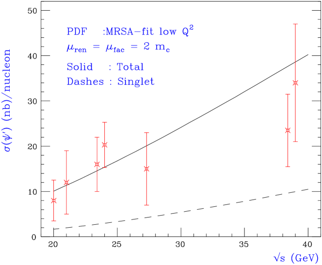
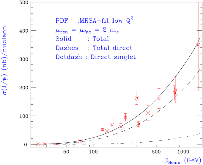
Figure 1: Left: Total $\psi^{\prime}$ (left) and $\psi$ (right) production in proton-nucleon collisions ($x_{F}>0$ only). For the $\psi$, the total cross section includes the radiative feed-down from $\chi_{cJ}$ and $\psi^{\prime}$. The solid lines are obtained with ${\cal M}^{\mbox{$\psi^{\prime}$}}_{6.4}=2.6\cdot 10^{-2}\;\mbox{$\mathrm{GeV}$}^{3}$ and ${\cal M}^{\psi}_{6.4}=1.8\cdot 10^{-2}\;\mbox{$\mathrm{GeV}$}^{3}$ for $\psi^{\prime}$ and $\psi$ respectively.

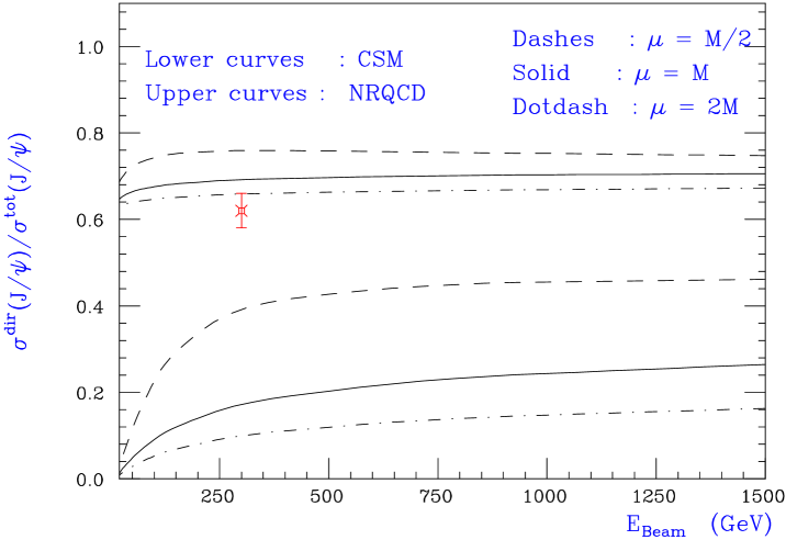
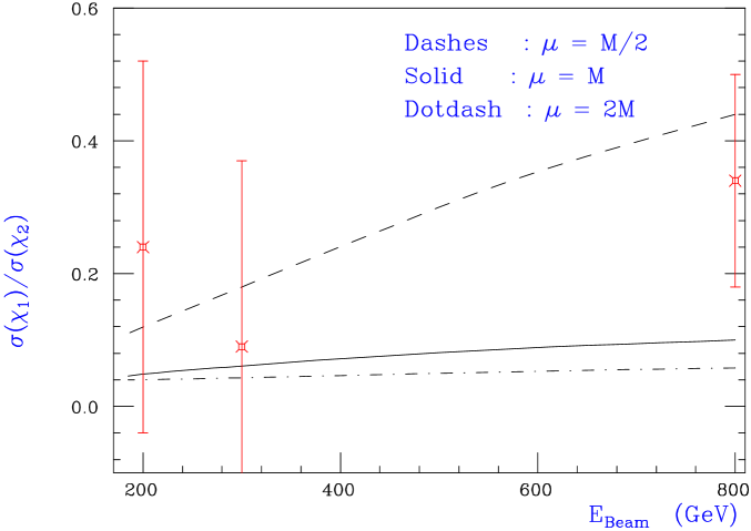
Figure 2: Ratio of direct to total $J\!/\!\psi$ (left) and $\chi_{c1}/\chi_{c2}$ (right) production in proton-nucleon collisions as a function of the beam energy. The experimental value at $300\;\mbox{$\mathrm{GeV}$}$ for $\sigma^{\rm dir}(\mbox{$J\!/\!\psi$})/\sigma^{\rm tot}(\mbox{$J\!/\!\psi$})$ is $0.62\pm 0.04$.

In the following we have used the low-$Q^{2}$ MRSA set of parton densities; $\!{}^{{\bf?}}$ $m_{c}=1.5\;\mbox{$\mathrm{GeV}$}$ ; the renormalization, factorization and NRQCD scales set equal to ${\mbox{$\mu_{R}$}}=\mbox{$\mu_{\rm F}$}={\mu_{\Lambda}}=2m_{c}$; the strong coupling, $\alpha_{s}$, tuned to the one used by the PDF set, i.e., $\Lambda_{\rm QCD}^{5}=152\;\mbox{$\mathrm{MeV}$}$; and the MEs collected in Table 3 as input values in the fits. Within the above choices the only free parameter left is the linear combination of MEs

$${\cal M}^{H}_{k}=\mbox{$\langle 0|{\cal O}_{1}^{H}(^{1}S_{0})|0\rangle$}+k\frac{\mbox{$\langle 0|{\cal O}_{1}^{H}(^{3}P_{J})|0\rangle$}}{m_{c}^{2}},$$ (48)

with $k=7$ for the LO analysis and $k\simeq 6.4$ at NLO. The results of the fit are shown in Fig. 1 and give:

$${\cal M}^{\rm NLO}_{6.4}({}^{1}\!S_{0}^{[8]},{}^{3}\!P_{J}^{[8]})=\left\{\begin{array}[]{c}\,\,\,1.8\cdot 10^{-2}\,\mbox{GeV}^{3}\qquad(J/\psi)\\ 0.26\cdot 10^{-2}\,\mbox{GeV}^{3}\qquad(\psi^{\prime}).\end{array}\right.$$ (49)

to be compared with the LO results of $\!{}^{{\bf?}}$

$${\cal M}^{\rm LO}_{7}({}^{1}\!S_{0}^{[8]},{}^{3}\!P_{J}^{[8]})=\left\{\begin{array}[]{c}\,\,\,3.0\cdot 10^{-2}\,\mbox{GeV}^{3}\qquad(J/\psi)\\ 0.52\cdot 10^{-2}\,\mbox{GeV}^{3}\qquad(\psi^{\prime}).\end{array}\right.$$ (50)

As expected, the inclusion of NLO corrections significantly reduces the values needed for the color-octet MEs. Unfortunately, the same sources of uncertainties present at LO, which are both theoretical (the strong dependence of the results on the choice of the heavy-quark mass and on the scale (which is only slightly improved at these energies)) and experimental (nuclear dependence, limited $x_{F}$ range, presence of elastically-produced charmonia) make it difficult to associate reliable errors to the fitted values.

Nevertheless, since most of these uncertainties should cancel in the ratios of cross-sections, we have also compared

$$R_{\chi} = \frac{\sigma(\chi_{c1})}{\sigma(\chi_{c2})}\qquad R_{\psi}=\frac{\sigma^{\rm dir}(\mbox{$J\!/\!\psi$})}{\sigma^{\rm tot}(\mbox{$J\!/\!\psi$})}$$ (51)

where

$$\sigma^{\rm tot}(\mbox{$J\!/\!\psi$})=\sigma^{\rm dir}(\mbox{$J\!/\!\psi$})+{\rm Br}(\mbox{$\psi^{\prime}$}\to\mbox{$J\!/\!\psi$})\,\sigma(\mbox{$\psi^{\prime}$})+\sum_{J}{\rm Br}(\chi_{cJ}\to\mbox{$J\!/\!\psi$})\,\sigma(\mbox{$\chi_{cJ}$})\,,$$ (52)

with the available experimental data (see Ref. $\!{}^{{\bf?}}$ for details). These are shown in Fig. 2. While the color-singlet approximation for $R_{\psi}$ is rather uncertain and clearly disfavored by the data, both the LO and the NLO NRQCD predictions show a much better agreement. Moreover, the NLO result turns out to be quite stable under scale variations. With a certain confidence, this result can be considered a remarkable success of the NRQCD approach.

Process	Ref.	$\langle{\cal O}_{8}^{\psi}(^{3}S_{1})\rangle$	$k$	${\cal M}^{\psi}_{k}$	$\langle{\cal O}_{8}^{\psi^{\prime}}(^{3}S_{1})\rangle$	${\cal M}^{\psi^{\prime}}_{k}$
Tevatron	$\!{}^{{\bf?}}$	$0.66$	$3$	$6.6$	$0.46$	$1.8$
	$\!{}^{{\bf?}}$	$1.06$	$3.5$	$4.4$	$0.44$	$1.8$
	$\!{}^{{\bf?}}$	$0.3$	$3$	$1.4$	$0.14$	$0.33$
	$\!{}^{{\bf?}}$	$0.4$	$3.5$	$6.6$	$0.36$	$0.78$
	$\!{}^{{\bf?}}$	$1.2$	$3.5$	$4.5$	$0.5$	$1.9$
Fixed-target	$\!{}^{{\bf?}}$	$(0.66)$	$7$	$3.0$	$(0.46)$	$0.52$
hadropr.	∗	$(1.06)$	$6.4$	$1.9$	$(0.44)$	$0.28$
B-decay	$\!{}^{{\bf?}}$	$(1.06)$	$3.1$	$1.5$	$(0.44)$	$0.6$

Table 4: Color octet matrix elements for $\psi$ and $\psi^{\prime}$ production as extracted from various analysis (${}^{*}=$ this work). Values in $10^{-2}\;{\rm GeV}^{3}$. Numbers in parenthesis are taken as input values.

The above analysis shows that, if on the one hand the NRQCD approach gives a rather consistent description of the data, on the other hand it is rather difficult to extract precise information on the color-octet matrix elements from the measurements. In this respect, it is interesting to compare some of the extractions available in the literature with the one above. The relevant color-octet matrix elements for the $\psi$ and $\psi^{\prime}$ are summarized in Table 4. Even if the very basic assumptions of the cited works are often quite different (PDF choice, inclusion of initial-state radiation and/or $k_{T}$ effects, implementation of Altarelli-Parisi evolution, etc.) and considering the theoretical uncertainties previously mentioned, the overall picture is reasonably consistent.

4 Conclusions

I have presented some applications of the NRQCD formalism to the phenomenology of inclusive quarkonium decays and production. In $\Upsilon$ decays we have established the importance of color-octet contributions to the total hadronic decay widths. We have then argued that the present extractions of $\alpha_{s}$ from $\Upsilon$ decays have to be regarded with great care, at least until measurements of the relevant non-perturbative matrix elements on the lattice are available. In the other two examples, the $\chi_{cJ}$ decays and the charmonium production at fixed-target experiments, we have been able to extract information on the non-perturbative MEs directly from the data. In the former case, this has allowed us to make a prediction for the hadronic width of the $h_{c}$ charmonium state while in the latter case, we checked the universality of the MEs against the available results. The conclusion is that, considering the ‘light’ mass of the charm, the NRQCD approach works surprisingly well and the extracted MEs are of the order of magnitude predicted by the scaling rules. On the other hand, the uncertainties present both at the theoretical and experimental level prevent us from performing more precise tests of the most distinctive prediction of NRQCD, i.e., the universality of the non-perturbative matrix elements. To overcome the above limitations, more exclusive quantities are under study. The most exciting and promising one is the expectation that high-$p_{T}$ quarkonia produced at hadronic colliders should be transversely polarized. $\!{}^{{\bf?},{\bf?}}$ Preliminary data from CDF $\!{}^{{\bf?}}$ do not confirm this prediction and may indicate that quarkonium physics is ready for new, unexpected surprises (see, e.g., Ref. $\!{}^{{\bf?}}$ and references therein).

References

References

- [1]
- [2] G. T. Bodwin, E. Braaten and G. P. Lepage, Phys. Rev. D51 (1995) 1125 [hep-ph/9407339]; erratum ibid. D55 (1997) 5853.
-
[3]
For a nice introduction to NRQCD and quarkonium physics
see, e.g., B. Grinstein, hep-ph/9811264.
For reviews on quarkonium production processes see, e.g.:
E. Braaten, S. Fleming, and T. C. Yuan, Ann. Rev. Nucl. Part. Sci. 46 (1996) 197 [hep-ph/9602374]; M. Beneke, hep-ph/9703429; M. Krämer, hep-ph/9707449; M. Krämer, F. Maltoni, and M.A. Sanchis-Lozano, ‘Quarkonium Production’ in Ref. and references therein.
For a recent review on NRQCD, see, e.g., I. Rothstein, hep-ph/9911276.
For the latest developments on top-antitop threshold production see, e.g., A. Hoang et al., Eur.Phys.J.direct C3:1-22,2000 and references therein. - [4] F. Maltoni, Ph. D. Thesis, University of Pisa, 1999, unpublished.
- [5] A. Petrelli, M. Cacciari, M. Greco, F. Maltoni and M. L. Mangano, Nucl. Phys. B514, 245 (1998) [hep-ph/9707223].
- [6] G. P. Lepage, L. Magnea, C. Nakhleh, U. Magnea and K. Hornbostel, Phys. Rev. D46 (1992) 4052 [hep-lat/9205007].
- [7] S. J. Brodsky, D. G. Coyne, T. A. DeGrand and R. R. Horgan, Phys. Lett. B73, 203 (1978).
- [8] R. D. Field, Phys. Lett. B133, 248 (1983).
- [9] M. Kramer, Phys. Rev. D60, 111503 (1999) [hep-ph/9904416].
- [10] F. Maltoni and A. Petrelli, Phys. Rev. D59, 074006 (1999) [hep-ph/9806455].
- [11] G. T. Bodwin, E. Braaten and G. P. Lepage, Phys. Rev. D46, 1914 (1992) [hep-lat/9205006].
-
[12]
Crystal Ball Coll., R. A. Lee, SLAC-report-282, (1985),
Stanford University Ph. D. thesis, unpublished. - [13] V. Shelkov et al. [CLEO Collaboration], Phys. Rev. D50, 4265 (1994).
- [14] T. A. Armstrong et al. [E670 Collaboration], Phys. Rev. Lett. 70, 2983 (1993).
- [15] D. Bauer et al. [TPC/Two-Gamma Collaboration], Phys. Lett. B302, 345 (1993).
- [16] E835 Collab., R. Calabrese, in Proceedings of LEAP 98 Biennal Conference on Low Energy Antiproton Physics (1998).
- [17] M. Acciarri et al. [L3 Collaboration], Phys. Lett. B453, 73 (1999).
- [18] K. Ackerstaff et al. [OPAL Collaboration], Phys. Lett. B439, 197 (1998) [hep-ex/9808025].
- [19] J. Z. Bai et al. [BES Collaboration], Phys. Rev. Lett. 81, 3091 (1998).
- [20] T. A. Armstrong et al. [E760 Collaboration], Nucl. Phys. B373, 35 (1992).
- [21] C. Caso et al., Eur. Phys. J. C3, 1 (1998).
- [22] E. J. Eichten and C. Quigg, Phys. Rev. D52 (1995) 1726.
- [23] E. Eichten and K. Gottfried, Phys. Lett. B66, 286 (1977).
- [24] T. A. Armstrong et al. [E760 Collaboration], Phys. Rev. Lett. 68, 1468 (1992).
- [25] E835 Collab., in “Proposal to continue the study of charmonium spectroscopy in annihilations”, Fermilab Proposal, Dic. 1997.
- [26] M. Beneke, A. Signer and V. A. Smirnov, Phys. Rev. Lett. 80, 2535 (1998) [hep-ph/9712302].
- [27] A. Czarnecki and K. Melnikov, Phys. Rev. Lett. 80, 2531 (1998).
- [28] W. Keung and I. J. Muzinich, Phys. Rev. D27, 1518 (1983).
- [29] G. A. Schuler, hep-ph/9403387.
- [30] P. Labelle, G. P. Lepage and U. Magnea, Phys. Rev. Lett. 72, 2006 (1994) [hep-ph/9310208].
- [31] M. Gremm and A. Kapustin, Phys. Lett. B407, 323 (1997) [hep-ph/9701353].
- [32] P. B. Mackenzie and G. P. Lepage, Phys. Rev. Lett. 47, 1244 (1981).
- [33] E. Braaten, S. Fleming and T. C. Yuan, Ann. Rev. Nucl. Part. Sci. 46, 197 (1996) [hep-ph/9602374].
- [34] M. Beneke, hep-ph/9703429.
- [35] M. Krämer, hep-ph/9707449.
- [36] P. Cho and A. K. Leibovich, Phys. Rev. D53, 150 (1996) [hep-ph/9505329]. Phys. Rev. D53, 6203 (1996) [hep-ph/9511315].
- [37] M. Beneke and M. Krämer, Phys. Rev. D55, 5269 (1997).
- [38] B. Cano-Coloma and M. A. Sanchis-Lozano, Nucl. Phys. B508, 753 (1997) [hep-ph/9706270].
- [39] E. Braaten, B. A. Kniehl and J. Lee, hep-ph/9911436.
- [40] P. Nason et al., hep-ph/0003142.
- [41] M. Beneke and I. Z. Rothstein, Phys. Rev. D54, 2005 (1996) [hep-ph/9603400].
- [42] M. Beneke, F. Maltoni and I. Z. Rothstein, Phys. Rev. D59, 054003 (1999) [hep-ph/9808360].
- [43] A. D. Martin, W. J. Stirling and R. G. Roberts, Phys. Rev. D51, 4756 (1995) [hep-ph/9409410].
- [44] P. Cho and M. B. Wise, Phys. Lett. B346, 129 (1995) [hep-ph/9411303].
- [45] M. Beneke and I. Z. Rothstein, Phys. Rev. D54, 2005 (1996).
- [46] CDF Collaboration, hep-ex/0004027
- [47] J. Lee, these proceedings.