BAYESIAN ANALYSIS

Abstract

After making some general remarks, I consider two examples that illustrate the use of Bayesian Probability Theory. The first is a simple one, the physicist’s favorite “toy,” that provides a forum for a discussion of the key conceptual issue of Bayesian analysis: the assignment of prior probabilities. The other example illustrates the use of Bayesian ideas in the real world of experimental physics.

1 INTRODUCTION

“We don’t know all about the world to start with; our knowledge by experience consists simply of a rather scattered lot of sensations, and we cannot get any further without some a priori postulates. My problem is to get these stated as clearly as possible.”

Sir Harold Jeffreys, in a letter to Sir Ronald Fisher dated 1 March, 1934.

Scientific inference has led to the surest knowledge we have yet, paradoxically, there is still disagreement about how to perform it. The disagreement is both within as well as between camps, the principal ones being frequentist and Bayesian. If pressed, the majority of physicists would claim to belong to the frequentist camp. In practice, we belong to both camps: we are frequentists when we wish to appear “objective,” but Bayesian when to be otherwise is either too hard, or makes no sense. Until fairly recently, relatively few of us have been party to the frequentist Bayesian debate. And society is all the better for it! It is our pragmatism that has cut through the Gordian Knot and allowed scientific progress. However, we find ourselves performing ever more complex inferences that, in some cases, have real world consequences and we can no longer regard the debate as mere philosophical musings. Indeed, this workshop is a testimony to this loss of innocence.

All parties appear, at least, to agree on one thing: probability theory is a reasonable basis for a theory of inference. But notice the use of the word “reasonable.” That word highlights the chief cause of the disagreement: any theory of inference is inevitably subjective in the following sense: what one person regards as reasonable may be considered unreasonable by another and, unlike scientific theories, we cannot appeal to Nature to decide which of the many inference theories is best, nor which criteria are to be used. I used to think that biased estimates were bad. But while some of us strive mightily to create them others look on bewildered, wondering why on earth we work so hard to achieve a characteristic they consider irrelevant.

Physicists, quite properly, are deeply concerned about delivering to the world objective results. Therefore, anything that openly declares itself to be subjective is viewed with suspicion. Since Neyman’s theory of inference is billed as objective many of us regard it as reasonable and the Bayesian theory as unfit for scientific use. However, when one scrutinizes the Neyman theory, its “objectivity” proves to be of a very peculiar sort, as I hope to show. I then discuss the difficult issue of prior probabilities by way of a simple model. In the last section, I describe a realistic Bayesian analysis to illustrate a point: Bayesian methods are not only fit for scientific use, they are precisely what is needed to make maximal use of data.

But first here are some remarks about probability.

1.1 What is Probability?

Probability theory is a mathematical theory about abstractions called probabilities. Therefore, to put this theory to work we are obliged to interpret these abstractions. At least three interpretations have been suggested:

• propensity (Popper)

• degree of belief (Bayes, Laplace, Gauss, Jeffreys, de Finetti)

• relative frequency (Venn, Fisher, Neyman, von Mises).

In parentheses I have given the names of a few of the proponents. According to Karl Popper, an unbiased coin, when tossed, has a propensity of 1/2 to land heads or tails. The 1/2 is claimed to be a property of the coin. According to Laplace probability is a measure of the degree of belief in a proposition: given that you believe the coin to be unbiased your degree of belief in the proposition “the coin will land heads” is 1/2. Finally, according to Venn if the coin is unbiased the relative frequency with which heads appears in an infinite sequence of coin tosses is 1/2. Venn seems to have the edge on the other two interpretations since it is a matter of experience that a coin tossed repeatedly lands heads about 1/2 the time as the number of tosses, that is, trials, increases. Every physicist who performs repeated controlled experiments, either real ones or virtual ones on a computer, provides overwhelming evidence in support of Venn’s interpretation.

So, which is it to be: degree of belief or relative frequency? The answer, I believe, is both, which prompts another question: is one interpretation more fundamental than the other and if so which? The answer is yes, degree of belief. It is yes for two very important reasons: one is practical the other foundational. The practical reason is that we use probability in a much broader context than that to which the relative frequency interpretation pertains. It has been amply demonstrated that we perform inferential reasoning according to rules that are isomorphic to those of probability theory. Any theory of inference that dismisses the “degree of belief” interpretation would be expected to suffer a severely restricted domain of applicability relative to the large domain in which probability is used in everyday life.

The second reason is that the Venn limit—the convergence of the ratio of the number of successes to the number of trails—cannot be proved without appealing to the notion of degree of belief[1]. The issue here is one of epistemology. Empirical evidence, even when overwhelming, does not prove that a thing is true; only that it is very likely, which is just another way of saying it is very probable. It is easy to see why a mathematical proof, as commonly understood, cannot be established. Consider a sequence of trials to test the Standard Model. Suppose each trial to be a proton anti-proton collision at the Tevatron. Each trial ends in success (a top quark is created) or failure. Let $T$ be the number of trials and $S$ the number of successes. Given the top quark mass, the Standard Model predicts the probability $p$ of successes. The Standard Model, we note, is a quantum theory. Therefore, the sequence of successes is strictly non-deterministic, in a sense in which a coin toss and a pseudo-random number generator are not.

However, a necessary (but of course not sufficient) basis for a mathematical proof of convergence of a sequence to a limit is the existence of a rule that connects term $T+1$ deterministically to $T$. But for quantum theory it is believed that no such rule exists. What can be and has been proved, by several people starting with James Bernoulli, is this:

If the order of trials is unimportant (that is, the sequence of trials is exchangeable), and if the probability of success at each trial is the same, then $S/T\rightarrow p$, as $T\rightarrow\infty$ with probability one.

At this point, I can adopt two attitudes regarding this theorem: one is that clarity of thought is a virtue; the second is that clarity of thought is nice but less important than pragmatism. As a pragmatist I would say that this theorem proves that the Venn limit exists. But in this case I prefer clarity. Let us, therefore, be clear about what this theorem actually proves and what it does not. Bernoulli’s theorem does not prove that $S/T$ converges to $p$. Rather it is a statement about 1) the probability that $S/T$ converges to $p$ as 2) the number of trials increases without limit, provided that 3) the order of trials does not matter and that 4) the probability at each trial is the same. Lurking behind these four seemingly innocuous statements are deep issues that are far beyond the scope of what I wish to say in this paper. Let me just note that the word “probability” occurs twice in the statement of Bernoulli’s theorem. If we insist that all probabilities are relative frequencies then we would have to interpret “probability of success at each trial” and “probability one” as the “limit with probability one” of other exchangeable sequences in order to be consistent. This leads into the abyss of an infinitely recursive definition. Doubtless, von Mises was well aware of this difficulty, which may be why he took the existence of the Venn “limit” as an axiom. However, even if one is prepared to accept this axiom, I do not think it circumvents the epistemological difficulty of defining a thing, probability, by making use of the thing twice in its definition. As de Finetti[2] puts it

“In order for the results concerning frequencies to make sense, it is necessary that the concept of probability, and the concepts deriving from it which appear in the statements and proofs of these results, should have been defined and given meaning beforehand. In particular, a result which depends on certain events being uncorrelated, or having equal probabilities, does not make sense unless one has defined in advance what one means by the probabilities of the individual events.”

I agree.

The alternative interpretation of probability is degree of belief. Thus the probability $p$ is our assessment of the probability of success at each trial, based on our current state of knowledge. That state of knowledge could be informed, for example, by the predictions of the Standard Model. Bernoulli’s theorem says that if our assessment of the probability of success at each trial is correct, and if our assessment does not change, then it is reasonable to expect $S/T\rightarrow p$ as $T\rightarrow\infty$.

But what if our assessment, initially, is incorrect? This poses no difficulty. As our state of knowledge changes, by virtue of data acquired, our assessment of the probability of success changes accordingly. Bayes’ theorem shows how the degree of belief of a coherent reasoner will be updated to the point where it closely matches the relative frequency $S/T$.

1.2 Neyman’s Theory

Neyman rejected the Bayesian use of Bayes’ theorem arguing that the prior probability for a parameter “has no meaning” when the latter is an unknown constant. He further argued that even if the parameters to be estimated could be considered as random variables we usually do not know the prior probability. With the benefit of hindsight, we can see that these arguments betray a confusion about of the notion of degree of belief. Jeffreys[1] frequently lamented the failure of his contemporaries to really understand what he was talking about. I would note that even amongst this illustrious gathering the confusion persists. So let me belabor a point: when one assigns a probability to a parameter it is not because one deems it sensible to think of the parameter as if it were a random variable—this is clearly nonsense if the parameter is in fact a constant. The probability assignments merely encode one’s knowledge (or that of an idealized reasoner) of the possible values of the parameter.

In his classic paper of 1937[3], Neyman introduced his theory of confidence intervals, which he believed provided an important element of an objective theory of inference. He not only specified the property that confidence intervals had to satisfy but he also gave a particular rule for constructing them, although he left considerable freedom that can be creatively exploited[4]. Neyman’s theory is elegant and powerful. Nonetheless, his theory is open to criticism. But in order to raise objections we need to understand what Neyman said.

Imagine an ensemble of trials, or experiments, $\{E\}$ to each of which we associate an interval $[\underline{\theta}(E),\overline{\theta}(E)]$. The ensemble of experiments yields an ensemble of intervals. Neyman required the ensemble of confidence intervals to satisfy the following condition:

For every possible fixed point $(\theta,\alpha)$ in the parameter space of the problem, where $\theta$ is the parameter of interest and $\alpha$ denotes all other parameters of the problem

$${\rm Prob}\{\theta\in[\underline{\theta}(E),\overline{\theta}(E)]\}\geq\beta.$$ (1)

According to Neyman this probability is to be interpreted as a relative frequency. Thus, any set of intervals is an ensemble of confidence intervals if the relative frequency with which the intervals contain the point $\theta$ is greater than or equal to $\beta$, for every possible fixed point in the parameter space regardless of its dimensionality. Neyman’s idea is intuitively clear: an interval picked at random from such an ensemble, the proverbial urn of sampling theory, will have a $100\beta$% chance of containing the fixed point $\theta$, whatever the value of $\theta$ and $\alpha$. This is a remarkable requirement. Here is an example.

Suppose we wish to measure a cross section. Our inference problem depends upon the following parameters: the cross section $\sigma$, the efficiency $\epsilon$, the background $b$ and the integrated luminosity $L$. Consider a fixed point $(\sigma,\epsilon,b,L)$ in the parameter space. To this point we associate an ensemble of confidence intervals, induced by an ensemble of possible experimental results. Some of these intervals $[\underline{\sigma}(E),\overline{\sigma}(E)]$ will contain $\sigma$, others will not. The fraction of intervals, in the ensemble, that contain $\sigma$ is called the coverage probability of the ensemble of intervals. A coverage probability is associated with every point $(\sigma,\epsilon,b,L)$ of the parameter space. Moreover, the value of the coverage probability may vary from point to point. Neyman’s key idea is that the ensembles of intervals should be constructed so that, over the allowed parameter space, the coverage probability never falls below some number $\beta$, called the confidence level. Both the coverage probability and the confidence level are to be interpreted as relative frequencies.

The parameter space and its set of ensembles form what mathematicians call a fibre bundle. The parameter space is the base space to each point of which is attached a fibre, that is, another space, here the ensemble of intervals associated with that parameter point. Each fibre has a coverage probability, and none falls below the confidence level $\beta$. Since the fibres may vary in a non-trivial way from point to point it is not possible, in general, to construct the fibre bundle as a simple Cartesian product of the parameter space and a single ensemble of intervals. In general, a non-trivial fibre bundle is the natural mathematical description of Neyman’s construction. Well natural if, like me, you like to think of things geometrically!

There are two difficulties with Neyman’s idea. The first is technical. For one-dimensional problems, or for problems in which we wish to set bounds on all parameters simultaneously, the construction of confidence intervals is straightforward. But when the parameter space is multi-dimensional and our interest is to set limits on a single parameter no general algorithm is known for constructing intervals. That is, no general algorithm is known for eliminating nuisance parameters. In our example, we care only about the cross-section; we have no interest in setting bounds on the integrated luminosity. What we do, in practice, is to replace the nuisance parameters with their maximum likelihood estimates. The justification for this procedure is the following theorem:

$$-2\log\frac{Pr(x|\theta,\hat{\alpha})}{Pr(x|\hat{\theta},\hat{\alpha})}\rightarrow\chi^{2},$$ (2)

as the data sample $x$ grows without limit, and provided that the maximum likelihood estimates $\hat{\theta}$ and $\hat{\alpha}$ lie within the parameter space minus its boundary.

If our data sample is sufficiently large its likelihood becomes effectively a (non-truncated) multi-variate Gaussian, and consequently the distribution of the log-likelihood ratio is $\chi^{2}$. Since that distribution is independent of the true values of the parameters a probability statement about the log-likelihood ratio can be re-stated as one about the parameter $\theta$. But, and this is the crucial point, the theorem is silent about what to do for small samples. Unfortunately, we high energy physicists insist on looking for new things, so our data samples are often small. So what are we, in fact, to do? We must after all publish. Today, with our surfeit of computer time, we can contemplate a brute-force approach: start with an approximate set of intervals, computed using Eq. (2), and adjust them iteratively until they make Neyman happy. But because of the second difficulty I now discuss the effort seems hardly worth the trouble.

The second difficulty is conceptual. It has been argued at this workshop, and elsewhere[5], that the set of published 95% intervals constitute a bona fide ensemble of approximately 95% confidence intervals. Here is the argument. Each published interval is drawn from an urn (that is, an ensemble of experiments if you prefer a more cheerful allusion) whose confidence level is 95%. The fact that each urn is completely different is irrelevant provided that the sampling probability from each is the same, namely 95%. Thus 95% of the set of published intervals will be found to yield true statements. And herein lies the beauty of coverage! The flaw in this argument is this: each published interval is drawn from an urn that does not objectively exist, because the ensemble into which an actual experiment is embedded is a purely conceptual construct not open to empirical scrutiny. Fisher[6], not known for fawning over Bayesians, made a similar point a long time ago:

“.. if we possess a unique sample on which significance tests are to be performed, there is always … a multiplicity of populations to each of which we can legitimately regard our sample as belonging; so the phrase ‘repeated sampling’ from the same population does not enable us to determine which population is to be used to define the probability level, for no one of them has objective reality, all being products of the statistician’s imagination.”

This is true of our ensemble of experiments. Consequently, a few troublesome physicists, bent on giving the Particle Data Group a hard time, need merely imagine a different set of urns from which the published results could legitimately have been drawn and thereby alter the confidence level of each result!

Of course, the published intervals do have a coverage probability. My claim is that its value is a matter to be decided by actual inspection—provided, of course, we know the right answers! It is not one that can be deduced a priori for the reason just given. The fact that I am able to construct ensembles of confidence intervals on my computer, by whatever procedure, and verify that they satisfy Neyman’s criterion is certainly satisfying, but in no way does it prove anything empirically verifiable about the interval I publish. Forgive me for flogging a sincerely dead horse, but let me state this another way: Since I do not repeat my experiment, any statement to the effect that the virtual ensemble simulated on my computer mimics the potential ensemble to which my published interval belongs is tantamount to my claiming that if I were to repeat my experiment, then I would do so such that the virtual and real ensembles matched. Maybe, or maybe not!

To summarize: A frequentist confidence level is a property of an ensemble, therefore, its objectivity, or lack thereof, is on par with the ensemble that defines it.

This whole discussion may strike you as a tad surreal, but I think it goes to the heart of the matter: many physicists, for sensible reasons, reject the Bayesian theory and embrace coverage because it is widely viewed as objective. But as argued above confidence levels may or may not be objective depending on the circumstances. Therefore, when confronted with a difficult inference problem our choice is not between an “objective” and “subjective” theory of inference, but rather between two different subjective theories. It may be reasonable to continue to insist upon coverage, but not because it is objective.

After this somewhat philosophical detour it is time to turn to the real world. But en route to the real world, lest Bayesians begin to feel uncontrollably smug, I’d like to discuss an instructive “toy” model that highlights the fact that for a Bayesian life is hardly a bed of roses[8].

2 THE PHYSICIST’S FAVOURITE TOY

The typical high energy physics experiment consists of doing a large number $T$ of similar things—for example, proton antiproton collisions, and searching for $n$ interesting outcomes—for example, $t\bar{t}$ production. We invariably assume that the order of the collisions is irrelevant and that each interesting outcome occurs with equal probability. Then we may avail ourselves of the well-known fact that the probability assigned to $n$ outcomes out of $T$ trials, with our assumptions, is binomial. Since $n<<T$, this probability can be approximated by a Poisson distribution

$${\rm Pr}(n|\mu,I)=\frac{e^{-\mu}\mu^{n}}{n!},$$ (3)

and thus do we arrive at the physicist’s favourite toy. The symbol $I$ denotes all prior information and assumptions that led us to this probability assignment. Here, it is introduced for pedagogical reasons; to remind us of the fact that all probabilities are conditional. We shall assume that our aim is to infer something about the Poisson parameter $\mu$, given that we have observed $n$ events. Just for fun, we’ll give this problem to each workshop member. Naturally, being physicists, each of us insists on parameterizing this problem as we see fit, but in the end when we compare notes we shall do so in terms of the parameter $\mu$, by transforming to that parameter.

There are, of course, infinitely many ways to parameterize a likelihood function and the Poisson likelihood is no exception. For simplicity, however, let’s assume that each of us uses a parameter $\mu_{p}$ related to $\mu$ as follows

$$\mu_{p}=\mu^{p}.$$ (4)

“$p$” for physicist if you like! In terms of the parameter $\mu_{p}$ Eq. (3) becomes

$${\rm Pr}(n|\mu_{p},I)=\frac{e^{-\mu_{p}^{1/p}}\mu_{p}^{n/p}}{n!},$$ (5)

which, we note, does not alter the probability assigned to $n$.

From Bayes’ theorem

$${\rm Post}(\mu_{p}|n,I)=\frac{{\rm Pr}(n|\mu_{p},I){\rm Prior}(\mu_{p}|I)}{\int_{\mu_{p}}{\rm Pr}(n|\mu_{p},I){\rm Prior}(\mu_{p}|I)},$$ (6)

each of us can make inferences about our parameter $\mu_{p}$, and hence $\mu$. Of course, no one can proceed without specifying a prior probability ${\rm Prior}(\mu_{p}|I)$. Unfortunately, being mere physicists we do not know what its form should be. But since we are all in the same state of knowledge regarding our parameter, coherence would seem to demand that we use the same functional form. So without a shred of motivation let’s try the following form for the prior probability

$${\rm Prior}(\mu_{p}|I)=\mu_{p}^{-q}d\mu_{p}.$$ (7)

Although this prior is plucked out of thin air, it is actually more general than it appears because, in principle, $q$ could be an arbitrarily complicated function of $p$. Now each of us is in a position to calculate, assuming that the allowed parameter space for $\mu_{p}$ is $[0,\infty)$. We each find that

$${\rm Post}(\mu_{p}|n,I)=\frac{e^{-\mu_{p}^{1/p}}\mu_{p}^{n/p-q}d\mu_{p}}{p\Gamma(n-pq+p)}.$$ (8)

But as agreed, each of us transforms our posterior probability to the parameter $\mu$ using Eq. (4). Thus we obtain, from Eq. (8),

$${\rm Post}(\mu|n,I)=\frac{e^{-\mu}\mu^{n-pq+p-1}d\mu}{\Gamma(n-pq+p)}.$$ (9)

Unfortunately, something is seriously amiss with the family of posterior probabilities represented by Eq. (9): each of us has ended up making a different inference about the same parameter $\mu$! We can see this more clearly by computing the $r$th moment

$$m_{r} \equiv \int_{\mu}\mu^{r}{\rm Post}(\mu|n,I)$$

$$= \Gamma(n-pq+p+r)/\Gamma(n-pq+p),$$

of the posterior probability ${\rm Post}(\mu|n,I)$. The moments clearly depend on $p$, that is, on how we have chosen to parameterize the problem.

What does a Bayesian have to say about this state of affairs? Is it a problem? I would say yes, it is. But there are some Bayesians who call themselves “subjective Bayesians” and others who believe themselves to be “objective Bayesians.” I confess that these terms leave me a bit baffled. The latter term because it seems to be an oxymoron and the former because it seems to be superfluous. The fundamental Bayesian pact is this: The prior probability is an encoding of a state of knowledge; as such it is a subjective construct. That construct may encode one’s personal state of knowledge or belief, and that’s a fine thing to do and is very powerful. But it may also encode a state of knowledge that is not specifically yours and that too is just fine. The issue is one of encoding a state of knowledge: Are there any desiderata that should be respected? The subjectivist is probably inclined to say no: simply choose the parameterization that makes sense for you and associate a prior, declare it to be supreme, and force all other priors to differ from yours in just the right way to render an inference about $\mu$ unique. So a “subjective” Bayesian would presumably reject Eq. (7).

I believe that to make headway, we should entertain some further principles. They should not degenerate into dogma but should serve as a lantern in the dark. Here are two possible principles:

• Possible Principle 1: For the same likelihood and the same form of prior we should obtain the same inferences.

• Possible Principle 2: The moments of the posterior probability should be finite.

Let’s apply these tentative principles to the moments in Eq. (2). Principle 1 says that each of us should make the same inferences about $\mu$, that is, the moments ought not to depend on the whim of a workshop member; it ought not to depend on $p$. Principle 2 says that $m_{r}<\infty$. Together these principles imply that

$$-pq+p=a>0,$$ (11)

where $a$ is a constant. This leads to the following prior

$${\rm Prior}(\mu_{p}|I)=\mu_{p}^{a/p-1}d\mu_{p}.$$ (12)

But we didn’t quite make it; our principles are insufficient to uniquely specify a value for the constant $a$. We need something more. Here is something more, suggested by Vijay Balasubramanian[7]:

• Possible Principle 3: When in doubt, choose a prior that gives equal weight to all likelihoods indexed by the same parameters.

That is, impose a uniform prior on the space of distributions. This requirement is a much more reasonable one (here is that word again) than imposing uniformity on the space of parameters because the space of distributions is invariant, whereas that of parameters is not. The space of distributions is akin to a space containing invariant objects like the vectors in a vector space, whereas the parameter space is analogous to the non-invariant space of vector coordinates. In our case, we impose a uniform prior on the space inhabited by Poisson distributions. Balasubramanian has shown that a uniform prior on the space of distributions induces, locally, a Riemannian metric whose invariant measure is determined by the Fisher Information, $F$. For our toy model the invariant measure is

$${\rm Prior}(\mu_{p}|I)=F^{1/2}d\mu_{p},$$ (13)

where

$$F(\mu_{p})=-\left<\frac{d^{2}\log{\rm Pr}(n|\mu_{p},I)}{d\mu_{p}^{2}}\right>.$$ (14)

Equation (13) is called the Jeffreys prior. It gives $a=1/2$ and thus uniquely specifies the form of the prior probability. Possible Principle 3 is a generalization of Possible Principle 1. Thus we conclude that the prior probability that forces us all to make the same inference, regardless of how we choose to parameterize the problem, is

$${\rm Prior}(\mu_{p}|I)=\mu_{p}^{-\frac{1}{2}(2-p)}d\mu_{p}.$$ (15)

This is all very tidy. However, when Jeffreys[1] applied his general prior probability to the Gaussian, treating both its mean and standard deviation together he got a result he did not like. He therefore suggested another principle:

• Possible Principle 4: If the parameter space can be partitioned into subspaces that, a priori, are considered independent then the general prior should be applied to each subspace separately.

This gave him a prior he liked. Alas, for a Bayesian life is not easy. While the frequentist struggles with justifying the use of a particular non-objective ensemble the Bayesian struggles to justify why some set of additional principles for encoding minimal prior knowledge is reasonable. Meanwhile, the “subjective Bayesian” says this is all a mere chasing after shadows. And so it goes!

3 THE READ WORLD

The foregoing discussion might suggest to “abandon all hope yea who enter” the real world of inference problems. Fortunately, it is not quite so bleak. The real world imposes some very severe constraints on what we can reasonably be expected to do. For one thing, the lifetime of a physicist is finite, indeed, short when compared with the age of the universe. Technical resources are also finite. And then there is competition from fellow physicists. Finally, uncertainty in abundance is the norm. Perhaps with enough deep thought all inference problems can be solved in a pristine manner. In practice, we are forced to exercise a modicum of judgement when undertaking any realistic analysis. We introduce approximations as needed, we side-step difficult issues by accepting some conventions and we rely upon our ability not to get lost amongst the trees. But when I reflect on what must be done to measure, say, the top quark mass, a problem replete with uncertainties in the jet energy scale, acceptance, background, luminosity, Monte Carlo modeling to name but a few, it strikes me as desirable to have a coherent and intuitive framework to think about such problems. Bayesian Probability Theory provides precisely such a framework. Moreover, it is a framework that mitigates our propensity to get confused about statistics when the going gets tough. The second example I discuss shows that real science can be done in spite of prior anxiety[8].

3.1 Measuring the Solar Neutrino Survival Probability

It has been known for over a quarter of a century that fewer electron neutrinos are received from the Sun than expected on the basis of the Standard Solar Model (SSM)[9, 10, 11, 12, 13]. This is the famous solar neutrino problem. Figure 1 summarizes the situation as of Neutrino 98.

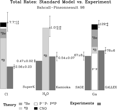
Figure 1: Predictions of the 1998 Standard Solar Model of Bahcall and Pinsonneault relative to data presented at Neutrino 98. Courtesy J.N. Bahcall.

If the SSM is correct—and there is very strong evidence in its favour[14], then the inevitable conclusion is that a fraction of the electron neutrinos created in the solar core are lost before they reach detectors on Earth. The loss of electron neutrinos is parameterized by the neutrino survival probability, $p(\nu|E_{\nu})$, which is the probability that a solar neutrino $\nu$ of energy $E_{\nu}$ arrives at the Earth.

Several loss mechanisms have been suggested, such as the oscillation of electron neutrinos to less readily observed states such as muon, tau or sterile neutrinos[15, 16]. Many $\chi^{2}$-based analyses have been performed to estimate model parameters[17, 18, 19]. To the degree that a fit to the solar neutrino data is good it provides evidence in favour of the particular new physics that has been assumed. From this perspective, solar neutrino physics is yet another way to probe physics beyond the Standard Model.

But I’d like to address a more modest question: What do the data tell us about the solar neutrino survival probability independently of any particular model of new physics? We can provide a complete answer by computing the posterior probability of different hypotheses about the value of the survival probability, for a given neutrino energy[21, 22]. Our Bayesian analysis is comprised of four components

• The model

• The data

• The likelihood

• The prior

First we sketch the model. (See Ref. [21] for details.)

The solar neutrino capture rate $S_{i}$ on chlorine and gallium can be written as

$$S_{i}={\sum_{j}}\Phi_{j}\int p(\nu|E_{\nu})\sigma_{i}(E_{\nu})\phi_{j}(E_{\nu})dE_{\nu},$$ (16)

where $\Phi_{j}$ is the total flux from neutrino source $j$, $\phi_{j}$ is the normalized neutrino energy spectrum and $\sigma_{i}$ is the cross section for experiment $i$. The predicted spectrum, plus experimental energy thresholds, are shown in Fig. 2. The full spectrum consists of eight components (of which six are shown in Fig. 2), with total fluxes $\Phi_{1}$ to $\Phi_{8}$[11].

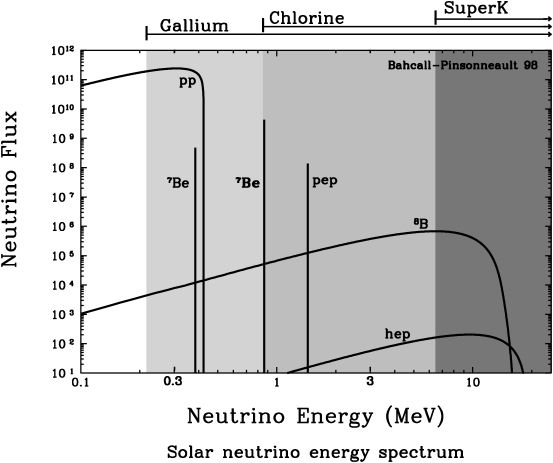
Figure 2: Solar neutrino energy spectrum as predicted by the Bahcall-Pinsonneault 1998 Standard Solar Model, including the neutrino energy thresholds for different solar neutrino experiments. Courtesy J.N. Bahcall.

The Super-Kamiokande experiment[23] measures the electron recoil spectrum arising from the scattering of the ${}^{8}B$ neutrinos (plus higher energy neutrinos) off atomic electrons. We shall use the electron recoil spectrum reported at Neutrino 98. The spectrum spans the range 6.5 to 20 MeV. Light water experiments, like Super-Kamiokande, are sensitive to all neutrino flavors but do not distinguish between them. There are, therefore, two possibilities: the $\nu_{e}$ deficit could be caused by $\nu_{e}$ conversions to $\nu_{x}$, where $x$ is either $\mu$ or $\tau$. If so the measured neutrino flux would be the sum of these flavors. If, however, the $\nu_{e}$ are simply lost without a trace, for example because of conversion into sterile neutrinos, then the measured flux would be comprised of $\nu_{e}$ only. Like the rates for the radiochemical experiments, the measured electron recoil spectrum is linear in the neutrino survival probability. The data are shown in Fig. 3.

Figure 3: Electron recoil spectrum measured by Super-Kamiokande compared to spectrum predicted by the Bahcall-Pinsonneault 1998 Standard Solar Model. From Ref. [24].

For solar neutrino experiments, a reasonable definition of sensitivity is the product of the cross section times the spectrum[21]. This quantity is plotted in Fig. 4. Two points are noteworthy: each experiment is sensitive to different parts of the neutrino energy spectrum and there are regions in neutrino energy where the sensitivity is essentially zero. We should anticipate that these facts will constrain what we are able to learn about the neutrino survival probability from the current solar neutrino data.

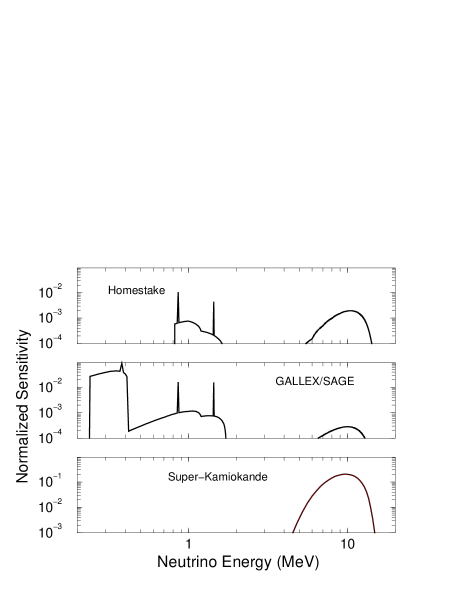
Figure 4: Spectral sensitivity as a function of the neutrino energy. From Ref. [21].

Since we do not know the cause of the solar neutrino deficit, let’s adopt a purely phenomenological approach to the survival probability. Guided by the results from previous analyses [17, 18, 19, 20] we write the survival probability as a sum of two finite Fourier series:

$$p(\nu|E_{\nu},a) = \sum_{r=0}^{7}a_{r+1}\mbox{cos}(r\pi E_{\nu}/L_{1})/(1+\mbox{exp}[(E_{\nu}-L_{1})/b])$$

$$+ \sum_{r=0}^{3}a_{r+9}\mbox{cos}(r\pi E_{\nu}/L_{2}),$$

where now we explicitly note the fact that the survival probability depends upon the set of parameters $a$. The first term in Eq. (3.1) is defined in the interval 0.0 to $L_{1}$ MeV—and suppressed beyond $L_{1}$ by the exponential. The second term spans the interval 0.0 to $L_{2}$ MeV. We have divided the function this way to model a survival probability that varies rapidly in the interval 0.0 to $L_{1}$ and less so elsewhere. The parameters $L_{1}$, $L_{2}$ and $b$ are set to 1.0, 15.0 and 0.1 MeV, respectively.

We now consider the likelihood function ${\rm Pr}(D|H,I)$, where $H$ denotes the hypothesis under consideration. The likelihood is assumed to be proportional to a multi-variate Gaussian $g(D|S,\Sigma)$, where $D\equiv(D_{1},\ldots,D_{19})$ represents the 19 data—3 rates from the chlorine and gallium experiments plus 16 rates from the binned Super Kamiokande electron recoil spectrum (Fig. 3); $\Sigma$ denotes the $19\times 19$ error matrix for the experimental data and $S\equiv(S_{1},\ldots,S_{19})$ represents the predicted rates.

The remaining ingredient is the prior probability. First we assess our state of knowledge. There are two sets of parameters to be considered: the total fluxes $(\Phi_{1},\ldots,\Phi_{8})$ and the survival probability parameters $(a_{1},\ldots,a_{12})$. The hypotheses under consideration concern the values of these two sets of parameters. The Standard Solar Model provides predictions $\Phi^{0}\equiv(\Phi_{1}^{0},\ldots,\Phi_{8}^{0})$ for the total fluxes, together with estimates of their theoretical uncertainties. So here is an analysis that must deal with theoretical uncertainties in some sensible way. I do not know how such a thing can be addressed in a manner consistent with frequentist precepts. For a Bayesian uncertainty is, well, uncertainty, regardless of provenance; therefore, every sort can be treated identically. We represent our state of knowledge regarding the fluxes by a multi-variate Gaussian prior probability ${\rm Prior}(\Phi|I)=$ $g(\Phi|\Phi^{0},\Sigma_{\Phi})$, where $\Phi^{0}$ is the vector of flux predictions and $\Sigma_{\Phi}$ is the corresponding error matrix[11].

Unfortunately, we know very little about the parameters $a_{1},\ldots,a_{12}$, so we shall short-circuit discussion by taking, as a matter of convention, the prior probability for $a$ to be uniform. In practice, any other plausible choice makes very little difference to our conclusions. We may even find that a uniform prior for $a$ is consistent with the generalized Jeffreys prior. Thus we arrive at the following prior for this inference problem:

$${\rm Prior}(a,\Phi|I) = {\rm Prior}(a|\Phi,I){\rm Prior}(\Phi|I)$$

$$= da{\rm Prior}(\Phi|I),$$

where $I$ now includes the prior information from the Standard Solar Model.

Now we can calculate! The posterior probability is given by

$${\rm Post}(a,\Phi|D,I)=\frac{{\rm Pr}(D|a,\Phi,I){\rm Prior}(a,\Phi|I)}{\int_{a,\Phi}{\rm Pr}(D|a,\Phi,I){\rm Prior}(a,\Phi|I)}.$$ (19)

But since we aren’t really interested in the total fluxes probability theory dictates that we just marginalize (that is, integrate) them away to arrive at the quantity of interest ${\rm Post}(a|D,I)$. Actually, what we really want is the probability of the survival probability for a given neutrino energy $E_{\nu}$! That is, we want

$${\rm Post}(p|D,I)=\int_{a}\delta(p-p(\nu|E_{\nu},a))P(a|D,I).$$ (20)

Figure 5 shows contour plots of ${\rm Post}(p|D,I)$ for the two cases considered, conversion to sterile and active neutrinos.

Our Bayesian analysis has produced a result that, intuitively, makes a lot of sense. As expected, given the sensitivity plot in Fig. 4, our knowledge of the survival probability is very uncertain between 1 and 5 MeV. In fact, the survival probability is tightly constrained in only two narrow regions: in the ${}^{7}Be$ region just below 1 MeV and another at around 8 MeV, near the peak of the ${}^{8}B$ neutrino spectrum. For neutrino energies above 12 MeV or so, the survival probability is basically unconstrained by current data.

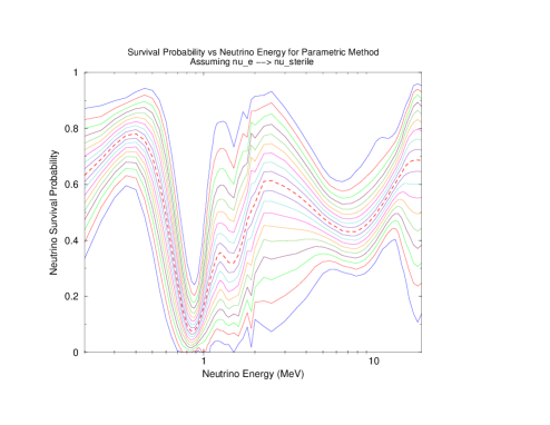
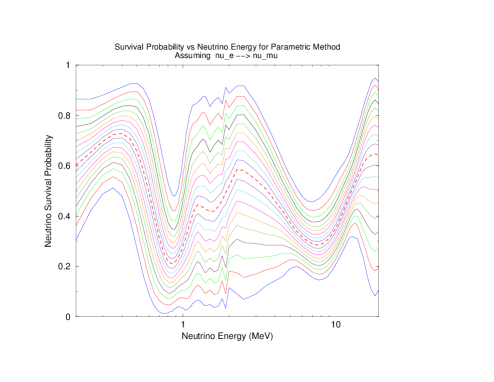
Figure 5: Survival probability vs neutrino energy assuming the neutrino flux consists of $\nu_{e}$ only (left plot) and $\nu_{e}$ to active neutrinos (right plot).

4 SUMMARY

It has been claimed by some at this workshop that Bayesian methods are of limited use in physics research. This of course is not true as I hope to have shown. Bayesian methods are, however, explicitly subjective and this may give one pause. I have argued that frequentist methods are not nearly as objective as claimed. While Bayesians cannot avoid the irreducible subjectivism of prior probabilities, frequentists cannot avoid the use of ensembles that do not objectively exist. Frequentists struggle with any uncertainty that does not arise from repeated sampling, like theoretical errors, while for Bayesians uncertainty in all its forms is treated identically. On the other hand, some Bayesians struggle to convince us that a particular choice of prior is reasonable, while frequentists look on in amusement. The point is neither approach is free from warts. But, of the two approaches to inference, I would say that the Bayesian one has more to offer, is easier to understand, has greater conceptual cohesion and, the most important point of all, more closely accords with the way we physicists think[25]. And this is real reason why it should be embraced.

References

- [1] H. Jeffreys,Theory of Probability, 3rd edition, Oxford University Press (1961). Chapters I, VII and VIII should be required reading for anyone who values clear thinking.
- [2] B. deFinetti, Theory of Probability, Vol. 1, John Wiley & Sons Ltd. (1990).
- [3] J. Neyman, Phil. Trans. R. Soc. London A236 (1937) 333. A beautiful paper, not nearly as daunting as one might imagine.
- [4] G. Feldman and R. Cousins, Phys. Rev. D57 (1998) 3873. A clear paper free of frequentist/Bayesian muddle! The authors make a sharp distinction between Bayesian and frequentist ideas and then opt for a principled frequentism.
- [5] R. Cousins, Am. J. Phys. 63 (1995) 398. An excellent accessible discussion about limits. And yes Bob, every physicist is a Bayesian, but many don’t know it! Ok, maybe Fred isn’t!
- [6] R. A. Fisher: An Appreciation (Lecture Notes on Statistics, Vol. 1), S. E. Fienberg and D. V. Hinkley, eds. Springer Verlag (1990). Lots of interesting historical stuff about Sir Ronald.
- [7] V. Balasubramanian, Statistical Inference, Occam’s Razor and Statistical Mechanics on The Space of Probability Distributions, Princeton University Physics Preprint PUPT-1587 (1996). Also available electronically as preprint cond-mat/9601030. The mathematics is a bit tricky, but the main ideas are not too hard to grasp. It’s worth a read.
- [8] R. E. Kass and L. Wasserman, J. Am. Stat. Assoc., 91 (1996) 1343. Life is tough!
- [9] T. A. Kirsten, Rev. Mod. Phys. 71 (1999) 1213.
-
[10]
J. N. Bahcall and Raymond Davis, Jr., An account of the
development of the solar neutrino problem, Essays in Nuclear
Astrophics, eds. C. A. Barnes, D. D. Clayton and D. Schramm,
Cambridge University Press (1982) pp. 243-285.
See also, //http://www.sns.ias.edu/jnb/Papers/Popular/snhistory.html - [11] J. N. Bahcall et al., Phys. Lett. B 433 (1998) 1.
- [12] J. N. Bahcall and M. Pinsonneault, Rev. Mod. Phys. 67 (1995) 781.
- [13] S. Turck-Chize and I. Lopes, Astrophys. J. 408 (1993) 347.
- [14] J. N. Bahcall, S. Basu and M. H. Pinsonneault, Phys. Lett. B 433 (1998) 1.
-
[15]
V.N. Gribov and B.M. Pontecorvo,
Phys. Lett. B 28 (1969) 493;
J.N. Bahcall and S.C. Frautschi, Phys. Lett. B 29 (1969) 623;
S.L. Glashow and L.M. Krauss, Phys. Lett. B 190 (1987) 199. -
[16]
L. Wolfenstein,
Phys. Rev. D 17 (1978) 2369;
S.P. Mikheyev and A.Yu. Smirnov, Sov. J. Nucl. Phys. 42 (1986) 913;
S.P. Mikheyev and A.Yu. Smirnov, Nuovo Cimento C 9 (1986) 17. - [17] N. Hata and P.Langacker, Phys. Rev. D 50 (1994) 632, N. Hata and P.Langacker, Phys. Rev. D 56 (1997) 6107.
-
[18]
Q. Y. Liu and S. T. Petcov,
Phys. Rev. D 56 (1997) 7392;
A.B. Balantekin, J.F. Beacom, J.M. Fetter, Phys. Lett. B 427 (1998) 317. - [19] S. Parke, Phys. Rev. Lett. 74 (1995) 839.
-
[20]
C.M. Bhat, 8th Lomonosov Conference on Elementary Particle
Physics, Moscow, Russia, August 1997, FERMILAB-Conf-98/066;
C.M. Bhat et al., Proceedings of the 9th Meeting of the DPF of the American Physical Society, ed. K. Heller et al., World Scientific (1996) 1220; - [21] C. M. Bhat, P. C. Bhat, M. Paterno and H. B. Prosper, Phys. Rev. Lett. 81 (1998) 5056.
- [22] E. Gates, L.M. Krauss, M. White, Phys. Rev. D 51 (1995) 2631.
-
[23]
K. Lande (Homestake), V.N. Gavrin (SAGE), T. Kirsten (GALLEX) and
Y. Suzuki (Super-Kamiokande), Neutrino 98, Proceedings XVIIIth
International Conference on Neutrino Physics and Astrophysics,
Takayama, Japan, June 1998, eds. Y. Suzuki and Y. Totsuka;
Robert Svoboda, private communication 1998. - [24] The Super-Kamiokande Collaboration, Phys. Rev. Lett. 82 (1999) 2644.
- [25] See for example, G. D’Agostini, Bayesian Reasoning In High-Energy Physics: Principles And Applications, CERN-99-03 (1999) 183.