Large $N$ Quantum Time Evolution Beyond Leading Order

Abstract

For quantum theories with a classical limit (which includes the large $N$ limits of typical field theories), we derive a hierarchy of evolution equations for equal time correlators which systematically incorporate corrections to the limiting classical evolution. Explicit expressions are given for next-to-leading order, and next-to-next-to-leading order time evolution. The large $N$ limit of $N$-component vector models, and the usual semiclassical limit of point particle quantum mechanics are used as concrete examples. Our formulation directly exploits the appropriate group structure which underlies the construction of suitable coherent states and generates the classical phase space. We discuss the growth of truncation error with time, and argue that truncations of the large-$N$ evolution equations are generically expected to be useful only for times short compared to a “decoherence” time which scales like $N^{1/2}$.

I Introduction

The time evolution of quantum systems away from equilibrium is of interest in many applications including, but certainly not limited to, phase transition dynamics, inflationary reheating, and heavy ion collisions. Large $N$ expansions have provided a widely used technique for studying equilibrium properties in statistical physics and field theory [1, 2, 3], and it is natural to apply a similar strategy for studying non-equilibrium problems. The large $N$ limit (as typically formulated) is actually a special type of classical limit [4]. Suitable observables behave classically and the quantum dynamics reduces to classical dynamics on an appropriate phase space.

Considerable work has been done examining the dynamics of far from equilibrium states in a variety of applications using leading large-$N$ time-evolution [5, 6, 7, 8, 9, 10]. A major virtue of large $N$ techniques (compared to alternative wholly uncontrolled approximation schemes) is that one should be able to improve the approximation by systematically including sub-leading effects suppressed by powers of $1/N$. For a variety of equilibrium problems (such as critical phenomena), this approach can work quite well [11, 12, 13].

For initial value problems, in which one would like to choose a non-equilibrium initial state and then examine the subsequent time evolution, traditional formulations of large-$N$ expansions using graphical or functional integral techniques [3] are very awkward. A major difficulty with these approaches is that they generate integral equations which are non-local in time when sub-leading $1/N$ corrections are retained. For practical (numerical) applications, one would vastly prefer a formulation in which locality in time is always preserved.

In this paper, we describe a formulation of large $N$ (or semi-classical) dynamics which leads to a coupled hierarchy of time-local evolution equations for equal time correlation functions. Our approach directly exploits the appropriate group structure underlying the construction of suitable coherent states and the existence of the classical limit [4]. We specifically focus on the time evolution of initial states chosen to equal one of these coherent states. We will give explicit next-to-leading order (NLO), and next-to-next-to-leading order (NNLO), expressions for the required evolution equations. Somewhat related hierarchies of evolution equations have been discussed in several recent papers [14, 15]. Because of our exploitation of the underlying group structure, the formulation we derive is more efficient, in the sense that it requires integration of fewer coupled equations at a given order in $1/N$.

A major question which we discuss, but do not fully resolve, is the propagation of errors induced by truncating the exact (infinite) hierarchy at a given order in $1/N$. It is known that the $N\to\infty$ limit is not uniform in time. For example, in typical large $N$ field theories the characteristic time scales for scattering or thermalization are known to scale as $N$ to some positive power. For a fixed time interval $t$, results obtained by integrating evolution equations truncated at, for example, next-to-leading order, will have only order $1/N^{2}$ errors. For sufficiently large $N$, and fixed $t$, including successively higher orders in the $1/N$ hierarchy will yield more accurate results. But for fixed $N$ and some given truncation of the $1/N$ hierarchy, it should be expected that the truncation error will grow with increasing time and eventually become order unity. A key question is how this “breakdown” time scales with $N$ and the order of the truncation. One might hope that a next-to-leading order approximation would be useful [that is, have at most ${\cal O}(1/N)$ global errors] for times of order $N$, while a next-to-next-to-leading order scheme would be useful out to times of order $N^{2}$, etc. But it is quite conceivable that errors in an order-$k$ truncation will grow with time like $(t^{\alpha}/N)^{k}$ for some positive $\alpha$, which would imply that all truncations break down after a time of order $N^{1/\alpha}$. This behavior, which we consider likely, may well depend on the specific theory and choice of initial state. Available numerical work, such as [14, 15], sheds little light on this issue. We discuss several examples where it is possible to argue that quantum “decoherence” produces exactly this type of limit on the range of validity of large $N$ truncations.

The paper is arranged as follows. The general framework which allows us to treat many theories with a classical limit in a uniform fashion is outlined in section II. This material is largely taken from Ref. [4]. Section III describes the particular class of operators we will consider, and examines the structure of their coherent state equal time correlators. Section IV presents the resulting time evolution equations and discusses error propagation. These general results are applied to the examples of point particle quantum mechanics, and a general $N$-component vector model, in section V. For point particle quantum mechanics, we argue that the decoherence time generically scales as $\hbar^{-1/2}$, while for vector models it should scale as $N^{1/2}$. A brief concluding discussion follows.

II Coherence Group and Coherent States

The following slightly abstract framework is applicable to typical large $N$ limits (including $O(N)$ or $U(N)$ invariant vector models, matrix models, and non-Abelian gauge theories), as well as the $\hbar\to 0$ limit of ordinary quantum mechanics [4].

Consider a quantum theory depending on some parameter $\chi$ (such as $\hbar$ or $1/N$). The Hilbert space (which may depend on $\chi$) will be denoted ${\cal H}_{\chi}$. The quantum dynamics is governed by a Hamiltonian which we will write as $(\hbar/\chi)\,\hat{H}_{\chi}$. This rescaling of the Hamiltonian will prove to be convenient, and makes the Heisenberg equations of motion take the form

$${d\over dt}\,\hat{A}={i\over\chi}\left[\hat{H}_{\chi},\hat{A}\right].$$ (1)

The following assumptions are a set of sufficient conditions implying that the $\chi\to 0$ limit is a classical limit.

Assume there is a Lie group $G$ (called the coherence group) which, for every value of $\chi$, has a unitary representation on ${\cal H}_{\chi}$, $G_{\chi}=\left\{D_{\chi}(u):u\in G\right\}$. The states generated by applying elements of the coherence group to some (normalized) base state $|0\rangle_{\chi}\in{\cal H}_{\chi}$,

$$|u\rangle_{\chi}\equiv D_{\chi}(u)\,|0\rangle_{\chi}\,,\qquad u\in G\,,$$ (2)

are called coherent states. The coherence group acts on these states in a natural way, $D_{\chi}(u^{\prime})\,|u\rangle_{\chi}=|u^{\prime}u\rangle_{\chi}$.

We assume that the coherence group $G_{\chi}$ acts irreducibly on the corresponding Hilbert space ${\cal H}_{\chi}$. In other words, no operator (except the identity) commutes with all elements of the coherence group. This condition automatically implies that the set of coherent states form an over-complete basis for the Hilbert space ${\cal H}_{\chi}$. It also implies that any operator acting on ${\cal H}_{\chi}$ may be represented as a linear combination of elements of the coherence group.

For any operator $\hat{A}$ acting in ${\cal H}_{\chi}$, we define its symbol $A_{\chi}(u)$ as the set of coherent state expectation values, $A_{\chi}(u)=\langle u|\hat{A}|u\rangle_{\chi}$, $u\in G$. We assume that the only operator whose symbol vanishes identically is the null operator. Thus, distinct operators have different symbols, which means that any operator can, in principle, be completely reconstructed solely from its diagonal matrix elements in the coherent state basis.

Classical observables will be associated with operators that remain non-singular as $\chi$ goes to zero, that is, whose coherent state matrix elements, $\langle u|\hat{A}|u^{\prime}\rangle_{\chi}/\langle u|u^{\prime}\rangle_{\chi}$, do not blow up as $\chi\rightarrow 0$ for all $u,u^{\prime}\in G$. Such operators are called classical.

Two coherent states $|u\rangle$ and $|u^{\prime}\rangle$ are termed classically equivalent (we will write $u\sim u^{\prime}$) if in the $\chi\rightarrow 0$ limit, one can not distinguish between them using only classical operators, i.e., $\lim_{\chi\rightarrow 0}A_{\chi}(u)=\lim_{\chi\rightarrow 0}A_{\chi}(u^{\prime})$ for all classical operators $\hat{A}$. We assume that the overlap between any two classically inequivalent coherent states decreases exponentially with $1/\chi$ in the $\chi\rightarrow 0$ limit.

Under these assumptions, one may show that the $\chi\rightarrow 0$ limit of this theory truly is a classical limit [4]. The assumptions hold for $O(N)$ or $U(N)$ invariant vector models, matrix models, and gauge theories [4]. The quantum dynamics reduces to classical dynamics on a phase space $\Gamma$ given by a coadjoint orbit of the coherence group. Formally, points in $\Gamma$ correspond to equivalence classes of coherent states, $\Gamma=\{[u]:u\in G\}$, with $[u]=\left\{u^{\prime}\in G:u\sim u^{\prime}\right\}$. The symplectic structure on the phase space is completely determined by the Lie algebra structure of the coherence group. The classical Hamiltonian is just the $\chi\to 0$ limit of the coherent state expectation of the quantum Hamiltonian,

$$h_{\rm cl}(u)=\lim_{\chi\rightarrow 0}\hat{H}_{\chi}(u)\,.$$ (3)

To have sensible classical dynamics this limit must exist, i.e., $\hat{H}_{\chi}$ must be a classical operator. (This is why it was convenient the rescale the Hamiltonian by $\hbar/\chi$.) The classical action is

$$S_{\rm cl}[u(t)]=\lim_{\chi\to 0}\int dt\>\langle u(t)|\,i\chi\,\partial_{t}-\hat{H}_{\chi}|u(t)\rangle_{\chi}\,.$$ (4)

Both the classical Hamiltonian (3) and the action (4) depend only on the equivalence class of the coherent state $|u\rangle$, and thus do define sensible dynamics on the classical phase space.

The preceding discussion is just a formalization of the usual picture of a classical limit. A quantum mechanical wave packet, with a width of order $\chi^{1/2}$, behaves classically in the $\chi\to 0$ limit, and may be associated with a point in the classical phase space. The equations of motion that govern the classical dynamics are just coherent state expectations of the original quantum evolution equations.

III Coherent State Expectations

As noted earlier, the irreducibility of the coherence group implies that all operators may be (formally) constructed from the generators of the coherence group. Consequently, for characterizing the structure, and time evolution, of any state, one may focus attention on equal-time expectation values of products of coherence group generators.

Let $g$ denote the Lie algebra of the coherence group $G$. Let $\{e_{i}\}$ be a basis of $g$. The commutator of basis elements defines the structure constants, $\left[e_{i},e_{j}\right]=if_{ij}^{k}\,e_{k}$. The generators $e_{i}$ themselves are not classical operators, but rather are $1/\chi$ times classical operators. For convenience, let $\hat{x}_{i}$ denote the rescaled generator which is a classical operator, $\hat{x}_{i}\equiv\chi e_{i}$.

Consider the coherent state expectation value of the monomial $\hat{x}_{i_{1}}\hat{x}_{i_{2}}\cdots\hat{x}_{i_{k}}$. We would like to find an expansion of this expectation value in powers of $\chi$. A convenient representation for our purposes involves subtracted expectations

$$g^{(k)}_{i_{1}i_{2}\cdots i_{k}} \equiv \langle(\hat{x}_{i_{1}}-x_{i_{1}})\cdots(\hat{x}_{i_{k}}-x_{i_{k}})\rangle\,,$$ (5)

where $\langle\cdots\rangle$ denotes an expectation in some coherent state, and $x_{i}\equiv\langle\hat{x}_{i}\rangle$ are the expectations of the rescaled generators $\hat{x}_{i}$. Subtracted and un-subtracted expectations are related by

$$\langle\hat{x}_{i_{1}}\cdots\hat{x}_{i_{k}}\rangle = x_{i_{1}}\cdots x_{i_{k}}\times\left\{1+\sum_{(l_{1},l_{2})}{g^{(2)}_{l_{1}l_{2}}\over x_{l_{1}}x_{l_{2}}}+\sum_{(l_{1},l_{2},l_{3})}{g^{(3)}_{l_{1}l_{2}l_{3}}\over x_{l_{1}}x_{l_{2}}x_{l_{3}}}+\cdots+{g^{(k)}_{i_{1}\cdots i_{k}}\over x_{i_{1}}\cdots x_{i_{k}}}\right\},$$ (6)

where the $n$-tuples $(l_{1},l_{2},...,l_{n})$ are ordered subsets of $\{i_{1},...,i_{k}\}$. (There is no $g^{(1)}$ term since $g^{(1)}_{i}\equiv\langle\hat{x}_{i}-x_{i}\rangle=0$.)

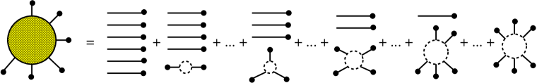
(a)         (b)        

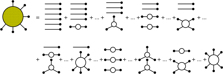
FIG. 1.: Expansion of the expectation a product of generators in terms of (a) subtracted, and (b) connected expectations. The shaded bubbles on the left denote full expectations of the product of generators. Each line with a dot on the end represents the expectation of a single generator. In (a), dashed-line bubbles correspond to subtracted $g^{(k)}$ expectations of strings of generators, while in (b) solid-line bubbles represent connected $s^{(k)}$ expectations. Ellipses ($\cdots$) denote ordered permutations of the preceding diagram.

Alternatively, one may expand in terms of connected expectations,

$$s^{(k)}_{i_{1}\cdots i_{k}}\equiv\langle\hat{x}_{i_{1}}\cdots\hat{x}_{i_{k}}\rangle^{\rm conn}\,.$$ (7)

The difference, illustrated graphically in Fig. 1, is that expansions in terms of connected expectations involve products of all possible ‘contractions’, while the terms in the expansion in subtracted expectations have only one string of generators ‘contracted’. The difference between subtracted and connected expectations first arises with four generators. Explicitly,

$$\langle\hat{x}_{i}\hat{x}_{j}\hat{x}_{k}\hat{x}_{l}\rangle = x_{i}x_{j}x_{k}x_{l}+x_{i}x_{j}\,g^{(2)}_{kl}+x_{i}x_{k}\,g^{(2)}_{jl}+x_{i}x_{l}\,g^{(2)}_{jk}+x_{k}x_{l}\,g^{(2)}_{ij}+x_{j}x_{l}\,g^{(2)}_{ik}+x_{j}x_{k}\,g^{(2)}_{il}$$ (10)

$$\quad{}+x_{i}\,g^{(3)}_{jkl}+x_{j}\,g^{(3)}_{ikl}+x_{k}\,g^{(3)}_{ijl}+x_{l}\,g^{(3)}_{ijk}+g^{(4)}_{ijkl}$$

$$= x_{i}x_{j}x_{k}x_{l}+x_{i}x_{j}\,s^{(2)}_{kl}+x_{i}x_{k}\,s^{(2)}_{jl}+x_{i}x_{l}\,s^{(2)}_{jk}+x_{k}x_{l}\,s^{(2)}_{ij}+x_{j}x_{l}\,s^{(2)}_{ik}+x_{j}x_{k}\,s^{(2)}_{il}$$ (12)

$$\quad{}+x_{i}\,s^{(3)}_{jkl}+x_{j}\,s^{(3)}_{ikl}+x_{k}\,s^{(3)}_{ijl}+x_{l}\,s^{(3)}_{ijk}+s^{(2)}_{ij}s^{(2)}_{kl}+s^{(2)}_{ik}s^{(2)}_{jl}+s^{(2)}_{il}s^{(2)}_{jk}+s^{(4)}_{ijkl}\,.$$

The coherent state overlap $\langle u|u^{\prime}\rangle_{\chi}$ is the generating functional for expectations of products of generators, since variations of the coherent state $u^{\prime}$ can bring down any desired generator of the Lie algebra, $\delta_{i}\,|u^{\prime}\rangle=e_{i}|u^{\prime}\rangle$. The logarithm of this overlap is therefore the generating functional for connected expectations. By assumption, $\ln\langle u|u^{\prime}\rangle_{\chi}$ is ${\cal O}(1/\chi)$ as $\chi\to 0$. This immediately implies that the $k$-th order connected expectation $s^{(k)}$ is ${\cal O}(\chi^{k-1})$. Note also that the commutator of functional derivatives is the functional derivative in the direction of the commutator,

$$\langle\cdots\hat{x}_{i}\hat{x}_{j}\cdots\rangle^{\rm conn}-\langle\cdots\hat{x}_{j}\hat{x}_{i}\cdots\rangle^{\rm conn}=\langle\cdots\left[\hat{x}_{i},\hat{x}_{j}\right]\cdots\rangle^{\rm conn}=i\chi\,f_{ij}^{m}\,\langle\cdots\hat{x}_{m}\cdots\rangle^{\rm conn},$$ (13)

or $s^{(k)}_{\cdots ij\cdots}-s^{(k)}_{\cdots ji\cdots}=i\chi\,f_{ij}^{m}\,s^{(k-1)}_{\cdots m\cdots}$.

By considering which connected expectations contribute to $g^{(k)}$, one may easily see that subtracted expectations fall off roughly half as fast as the connected ones, $g^{(2k)}\sim g^{(2k-1)}={\cal O}(\chi^{k})$. Because $g^{(k+2)}/g^{(k)}={\cal O}(\chi)$, expansion (6) is a power series in $\chi$, the parameter measuring how close the system is to being classical. Of course, subtracted expectations may always be rewritten in terms of connected expectations (and vice-versa). Ultimately, equations for connected expectations will be most useful. Nevertheless, using subtracted expectations as an intermediate representation is helpful because of the simple form of expansions in terms of subtracted expectations, as shown by Eq. (6) and Eq. (15) below. For later use, note that

$$g^{(k)}_{\cdots bijc\cdots}-g^{(k)}_{\cdots bjic\cdots}=i\chi\,f^{m}_{ij}\left(x_{m}\,g^{(k-2)}_{\cdots bc\cdots}+g^{(k-1)}_{\cdots bmc\cdots}\right).$$ (14)

Now consider an operator $V$ that can (at least formally) be expanded in powers of generators, $V=\sum_{k}\sum_{\{i_{1}\cdots i_{k}\}}\alpha_{i_{1}\cdots i_{k}}\,\hat{x}_{i_{1}}\cdots\hat{x}_{i_{k}}$, for some set of coefficients $\{\alpha_{i_{1}\cdots i_{k}}\}$. Operators of this form are well behaved for $\chi\rightarrow 0$, and so are good classical operators. Using (6),

$$\langle V\rangle = \sum_{k}\!\sum_{\{i_{1}\cdots i_{k}\}}\alpha_{i_{1}\cdots i_{k}}\,x_{i_{1}}\cdots x_{i_{k}}\left\{1+\sum_{(l_{1},l_{2})}{g^{(2)}_{l_{1}l_{2}}\over x_{l_{1}}x_{l_{2}}}+\sum_{(l_{1},l_{2},l_{3})}{g^{(3)}_{l_{1}l_{2}l_{3}}\over x_{l_{1}}x_{l_{2}}x_{l_{3}}}+\cdots+{g^{(k)}_{i_{1}\cdots i_{k}}\over x_{l_{1}}\cdots x_{l_{k}}}\right\}.$$ (15)

This can be packaged in an even more concise form,

$$\langle V\rangle=\bar{V}+g^{(2)}_{l_{1}l_{2}}\,V^{(l_{1}l_{2})}+g^{(3)}_{l_{1}l_{2}l_{3}}\,V^{(l_{1}l_{k}l_{3})}+g^{(4)}_{l_{1}l_{2}l_{3}l_{4}}\,V^{(l_{1}l_{k}l_{3}l_{4})}+{\cal O}(\chi^{3})$$ (16)

where summation on repeated indices is implied, and $\bar{V}\equiv\sum_{k}\sum_{\{i_{1}\cdots i_{k}\}}\alpha_{i_{1}\cdots i_{k}}\,x_{i_{1}}\cdots x_{i_{k}}$ is the number obtained by replacing each generator in $V$ by its coherent state expectation. Here we have introduced “ordered derivatives” $f^{(ij\cdots)}\equiv{\delta f\over\delta(x_{i}x_{j}\cdots)}$ defined by

$$f^{(l)} = {\partial\bar{f}\over\partial x_{l}}\,,$$ (18)

$$(fg)^{(l_{1}\cdots l_{k})} = \sum_{i=0}^{k}f^{(l_{1}\cdots l_{i})}g^{(l_{i+1}\cdots l_{k})}\,.$$ (19)

When acting on a string of generators, ordered derivatives produce a sum of products of expectations of the generators which remain after deleting the indicated generators, provided these appear (not necessarily contiguously) somewhere within the string in the order specified by the derivative. For example, ${\delta\over\delta(xp)}\,\hat{x}^{2}\hat{p}\hat{x}=2x^{2}$, and ${\delta\over\delta(xp)}\,\hat{x}\hat{p}\hat{x}^{2}\hat{p}=x^{2}p+2xpx+px^{2}=4x^{2}p$.

In the $\chi\to 0$ limit, coherent state expectations of the (rescaled) generators $\hat{x}_{i}$ turn into coordinates $x_{i}$ on the classical phase space and (classical) operators acting on ${\cal H}_{\chi}$ become functions on phase space, $\langle V\rangle=\bar{V}+O(\chi)$. For finite $\chi$, the successive terms in (16) precisely characterize the corrections to this classical limit.

IV Time Evolution

Since operators are completely determined by their symbols, to study the time dependence of any observable $\hat{A}$ it is sufficient to take the coherent state expectation value of its Heisenberg equation of motion (1),

$${d\over dt}\,\langle\hat{A}\rangle={i\over\chi}\left\langle\left[\hat{H}_{\chi},\hat{A}\right]\right\rangle.$$ (20)

In other words, we assume that the initial state is precisely some coherent state $|u\rangle$, and wish to determine the subsequent time evolution. To do so, we will first find an expansion, in powers of $\chi$, for the expectation of the commutator of classical operators.

A Symbols of Commutators

Consider classical operators $A$ and $B$ which (as in Section III) may be written as power series in the generators, $A=\sum\alpha_{i_{1}\cdots i_{m}}\,\hat{x}_{i_{1}}\cdots\hat{x}_{i_{m}}$, $B=\sum\beta_{j_{1}\cdots j_{n}}\,\hat{x}_{j_{1}}\cdots\hat{x}_{j_{n}}$. Their product is given by $AB=\sum\alpha_{i_{1}\cdots i_{m}}\beta_{j_{1}\cdots j_{n}}\hat{x}_{i_{1}}\cdots\hat{x}_{i_{m}}\hat{x}_{j_{1}}\cdots\hat{x}_{j_{n}}$. Using our previous result (16), we find

$$\langle AB\rangle = \bar{A}\bar{B}+g^{(2)}_{l_{1}l_{2}}\,(AB)^{(l_{1}l_{2})}+g^{(3)}_{l_{1}l_{2}l_{3}}\,(AB)^{(l_{1}l_{2}l_{3})}+g^{(4)}_{l_{1}l_{2}l_{3}l_{4}}\,(AB)^{(l_{1}l_{2}l_{3}l_{4})}+{\cal O}(\chi^{3})$$ (22)

$$= \bar{A}\bar{B}+s^{(2)}_{l_{1}l_{2}}\,(AB)^{(l_{1}l_{2})}+s^{(3)}_{l_{1}l_{2}l_{3}}\,(AB)^{(l_{1}l_{2}l_{3})}$$ (24)

$$\qquad\qquad\qquad{}+\left(s^{(2)}_{l_{1}l_{2}}\,s^{(2)}_{l_{3}l_{4}}+s^{(2)}_{l_{1}l_{3}}\,s^{(2)}_{l_{2}l_{4}}+s^{(2)}_{l_{1}l_{4}}\,s^{(2)}_{l_{2}l_{3}}\right)(AB)^{(l_{1}l_{2}l_{3}l_{4})}+{\cal O}(\chi^{3})$$

where now $(l_{1},l_{2},\cdots)$ denote ordered subsets of $\{i_{1},\cdots,i_{m},j_{1},\cdots,i_{n}\}$. We see from (IV A) that, to leading order, products of classical operators factorize, $\langle AB\rangle=\langle A\rangle\langle B\rangle+{\cal O}(\chi)$.

Using the expansion (IV A), and the reduction formulas for operator derivatives (III), one can evaluate the commutator. A generic term in the result will be

$$g^{(k)}_{l_{1}l_{2}\cdots l_{k}}\left[(AB)^{(l_{1}l_{2}\cdots l_{k})}-(BA)^{(l_{1}l_{2}\cdots l_{k})}\right]$$ (25)

$$= \phantom{-\;}g^{(k)}_{l_{1}\cdots l_{k}}\left(A^{(l_{1}\cdots l_{k})}\bar{B}+\cdots+A^{(l_{1}l_{2})}B^{(l_{3}\cdots l_{k})}+A^{(l_{1})}B^{(l_{2}\cdots l_{k})}+\bar{A}B^{(l_{1}\cdots l_{k})}\right)$$ (27)

$${}-g^{(k)}_{l_{1}\cdots l_{k}}\left(B^{(l_{1}\cdots l_{k})}\bar{A}+\cdots+B^{(l_{1}l_{2})}A^{(l_{3}\cdots l_{k})}+B^{(l_{1})}A^{(l_{2}\cdots l_{k})}+\bar{B}A^{(l_{1}\cdots l_{k})}\right)$$

$$= \phantom{+}\left(g^{(k)}_{l_{1}l_{2}l_{3}l_{4}\cdots l_{k}}-g^{(k)}_{l_{2}l_{3}l_{4}\cdots l_{k}l_{1}}\right)\left(A^{(l_{1})}B^{(l_{2}l_{3}l_{4}\cdots l_{k})}-B^{(l_{1})}A^{(l_{2}l_{3}l_{4}\cdots l_{k})}\right)$$ (30)

$$+\left(g^{(k)}_{l_{1}l_{2}l_{3}l_{4}\cdots l_{k}}-g^{(k)}_{l_{3}l_{4}\cdots l_{k}l_{1}l_{2}}\right)\left(A^{(l_{1}l_{2})}B^{(l_{3}l_{4}\cdots l_{k})}-B^{(l_{1}l_{2})}A^{(l_{3}l_{4}\cdots l_{k})}\right)$$

$$+\left(g^{(k)}_{l_{1}l_{2}l_{3}l_{4}\cdots l_{k}}-g^{(k)}_{l_{4}\cdots l_{k}l_{1}l_{2}l_{3}}\right)\left(A^{(l_{1}l_{2}l_{3})}B^{(l_{4}\cdots l_{k})}-B^{(l_{1}l_{2}l_{3})}A^{(l_{4}\cdots l_{k})}\right)+\cdots~{}.$$

The last term in the sum (25) is either $\left(g^{(2j)}_{l_{1}\cdots l_{j}l_{j+1}\cdots l_{2j}}-g^{(2j)}_{l_{j+1}\cdots l_{2j}l_{1}\cdots l_{j}}\right)\left(A^{(l_{1}\cdots l_{j})}B^{(l_{j+1}\cdots l_{2j})}\right)$ or $\left(g^{(2j+1)}_{l_{1}\cdots l_{j}l_{j+1}\cdots l_{2j+1}}-g^{(2j+1)}_{l_{j+1}\cdots l_{2j+1}l_{1}\cdots l_{j}}\right)$$\left(A^{(l_{1}\cdots l_{j})}B^{(l_{j+1}\cdots l_{2j+1})}-B^{(l_{1}\cdots l_{j})}A^{(l_{j+1}\cdots l_{2j+1})}\right),$ depending on whether $k$ is even or odd. Using (14) to reduce the differences $(g^{(k)}_{\cdots}-g^{(k)}_{\cdots})$ yields the final form for the expectation of the commutator of classical operators. The leading term is precisely the Poisson bracket on the classical phase space, while subsequent terms involve successively higher expectations $g^{(k)}$. Displaying subleading ${\cal O}(\chi)$ and ${\cal O}(\chi^{2})$ terms explicitly, one finds

$$\langle{1\over i\chi}\left[A,B\right]\rangle$$ (38)

$$\matrix{=\left[f^{m}_{l_{1}l_{2}}x_{m}\right]\left(A^{(l_{1})}B^{(l_{2})}\right)\hfill}\hskip 227.0312pt\Bigr{\}}\>{\cal O}(\chi^{0})$$

$$\left.\matrix{+\left[f^{m}_{l_{1}l_{2}}\,g_{ml_{3}}+f^{m}_{l_{1}l_{3}}\,g_{l_{2}m}\right]\left(A^{(l_{1})}B^{(l_{2}l_{3})}-B^{(l_{1})}A^{(l_{2}l_{3})}\right)\hfill\cr+\left[x_{m}\left(f^{m}_{l_{1}l_{2}}\,g_{l_{3}l_{4}}+f^{m}_{l_{1}l_{3}}\,g_{l_{2}l_{4}}+f^{m}_{l_{1}l_{4}}\,g_{l_{2}l_{3}}\right)\right]\left(A^{(l_{1})}B^{(l_{2}l_{3}l_{4})}-B^{(l_{1})}A^{(l_{2}l_{3}l_{4})}\right)\hfill\cr+\left[x_{m}\left(f^{m}_{l_{1}l_{3}}\,g_{l_{2}l_{4}}+f^{m}_{l_{1}l_{4}}\,g_{l_{3}l_{2}}+f^{m}_{l_{2}l_{3}}\,g_{l_{1}l_{4}}+f^{m}_{l_{2}l_{4}}\,g_{l_{3}l_{1}}\right)\right]\left(A^{(l_{1}l_{2})}B^{(l_{3}l_{4})}\right)\hfill}\hskip 29.19156pt\right\}{\cal O}(\chi^{1})$$

$$\left.\matrix{+\left[f^{m}_{l_{1}l_{2}}\,g_{ml_{3}l_{4}}+f^{m}_{l_{1}l_{3}}\,g_{l_{2}ml_{4}}+f^{m}_{l_{1}l_{4}}\,g_{l_{2}l_{3}m}\right]\left(A^{(l_{1})}B^{(l_{2}l_{3}l_{4})}-B^{(l_{1})}A^{(l_{2}l_{3}l_{4})}\right)\hfill\cr+\left[f^{m}_{l_{1}l_{3}}\,g_{ml_{2}l_{4}}+f^{m}_{l_{1}l_{4}}\,g_{l_{3}ml_{2}}+f^{m}_{l_{2}l_{3}}\,g_{l_{1}ml_{4}}+f^{m}_{l_{2}l_{4}}\,g_{l_{3}l_{1}m}\right]\left(A^{(l_{1}l_{2})}B^{(l_{3}l_{4})}\right)\hfill\cr+\left[x_{m}\left(f^{m}_{l_{1}l_{2}}\,g_{l_{3}l_{4}l_{5}}+f^{m}_{l_{1}l_{3}}\,g_{l_{2}l_{4}l_{5}}+f^{m}_{l_{1}l_{4}}\,g_{l_{2}l_{3}l_{5}}+f^{m}_{l_{1}l_{5}}\,g_{l_{2}l_{3}l_{4}}\right)\right.\hfill\cr\left.\hskip 12.91663pt+f^{m}_{l_{1}l_{2}}\,g_{ml_{3}l_{4}l_{5}}+f^{m}_{l_{1}l_{3}}\,g_{l_{2}ml_{4}l_{5}}+f^{m}_{l_{1}l_{4}}\,g_{l_{2}l_{3}ml_{5}}+f^{m}_{l_{1}l_{5}}\,g_{l_{2}l_{3}l_{4}m}\right]\hfill\cr\hskip 150.00023pt\times\left(A^{(l_{1})}B^{(l_{2}l_{3}l_{4}l_{5})}-B^{(l_{1})}A^{(l_{2}l_{3}l_{4}l_{5})}\right)\hfill\cr+\left[x_{m}\left(f^{m}_{l_{1}l_{3}}\,g_{l_{4}l_{5}l_{2}}+f^{m}_{l_{1}l_{4}}\,g_{l_{3}l_{5}l_{2}}+f^{m}_{l_{1}l_{5}}\,g_{l_{3}l_{4}l_{2}}+f^{m}_{l_{2}l_{3}}\,g_{l_{1}l_{4}l_{5}}+f^{m}_{l_{2}l_{4}}\,g_{l_{1}l_{3}l_{5}}\right.\right.\hfill\cr\left.\hskip 12.91663pt\left.+f^{m}_{l_{2}l_{5}}\,g_{l_{1}l_{3}l_{4}}\right)+f^{m}_{l_{1}l_{3}}\,g_{ml_{4}l_{5}l_{2}}+f^{m}_{l_{1}l_{4}}\,g_{l_{3}ml_{5}l_{2}}+f^{m}_{l_{1}l_{5}}\,g_{l_{3}l_{4}ml_{2}}+f^{m}_{l_{2}l_{3}}\,g_{l_{1}ml_{4}l_{5}}\right.\hfill\cr\left.\hskip 12.91663pt+f^{m}_{l_{2}l_{4}}\,g_{l_{1}l_{3}ml_{5}}+f^{m}_{l_{2}l_{5}}\,g_{l_{1}l_{3}l_{4}m}\right]\left(A^{(l_{1}l_{2})}B^{(l_{3}l_{4}l_{5})}-B^{(l_{1}l_{2})}A^{(l_{3}l_{4}l_{5})}\right)\hfill\cr+\left[x_{m}\left(f^{m}_{l_{1}l_{2}}\,g_{l_{3}l_{4}l_{5}l_{6}}+f^{m}_{l_{1}l_{3}}\,g_{l_{2}l_{4}l_{5}l_{6}}+f^{m}_{l_{1}l_{4}}\,g_{l_{2}l_{3}l_{5}l_{6}}+f^{m}_{l_{1}l_{5}}\,g_{l_{2}l_{3}l_{4}l_{6}}+f^{m}_{l_{1}l_{6}}\,g_{l_{2}l_{3}l_{4}l_{5}}\right)\right]\hfill\cr\hskip 150.00023pt\times\left(A^{(l_{1})}B^{(l_{2}l_{3}l_{4}l_{5}l_{6})}-B^{(l_{1})}A^{(l_{2}l_{3}l_{4}l_{5}l_{6})}\right)\hfill\cr+\left[x_{m}\left(f^{m}_{l_{1}l_{3}}\,g_{l_{4}l_{5}l_{6}l_{2}}+f^{m}_{l_{1}l_{4}}\,g_{l_{3}l_{5}l_{6}l_{2}}+f^{m}_{l_{1}l_{5}}\,g_{l_{3}l_{4}l_{6}l_{2}}+f^{m}_{l_{1}l_{6}}\,g_{l_{3}l_{4}l_{5}l_{2}}\right.\right.\hfill\cr\left.\left.\hskip 12.91663pt+f^{m}_{l_{2}l_{3}}\,g_{l_{1}l_{4}l_{5}l_{6}}+f^{m}_{l_{2}l_{4}}\,g_{l_{1}l_{3}l_{5}l_{6}}+f^{m}_{l_{2}l_{5}}\,g_{l_{1}l_{3}l_{4}l_{6}}+f^{m}_{l_{2}l_{6}}\,g_{l_{1}l_{3}l_{4}l_{5}}\right)\right]\hfill\cr\hskip 150.00023pt\times\left(A^{(l_{1}l_{2})}B^{(l_{3}l_{4}l_{5}l_{6})}-B^{(l_{1}l_{2})}A^{(l_{3}l_{4}l_{5}l_{6})}\right)\hfill\cr+\left[x_{m}\left(f^{m}_{l_{1}l_{4}}\,g_{l_{5}l_{6}l_{2}l_{3}}+f^{m}_{l_{1}l_{5}}\,g_{l_{4}l_{6}l_{2}l_{3}}+f^{m}_{l_{1}l_{6}}\,g_{l_{4}l_{5}l_{2}l_{3}}+f^{m}_{l_{2}l_{4}}\,g_{l_{1}l_{5}l_{6}l_{3}}+f^{m}_{l_{2}l_{5}}\,g_{l_{1}l_{4}l_{6}l_{3}}\right.\right.\hfill\cr\left.\left.\hskip 12.91663pt+f^{m}_{l_{2}l_{6}}\,g_{l_{1}l_{4}l_{5}l_{3}}+f^{m}_{l_{3}l_{4}}\,g_{l_{1}l_{2}l_{5}l_{6}}+f^{m}_{l_{3}l_{5}}\,g_{l_{1}l_{2}l_{4}l_{6}}+f^{m}_{l_{3}l_{6}}\,g_{l_{1}l_{2}l_{4}l_{5}}\right)\right]\left(A^{(l_{1}l_{2}l_{3})}B^{(l_{4}l_{5}l_{6})}\right)\hfill}\hfill\right\}{\cal O}(\chi^{2})$$

$$\left.\matrix{{}+{\cal O}(\chi^{3})\,.}\right.$$

B Equations of Motion

To determine the evolution to order ${\cal O}(\chi^{3})$, we need the time derivatives of $x_{i}(t)$, $g_{ij}(t)$, and $g_{ijk}(t)$. Take the commutator of products of generators with the Hamiltonian and subtract the disconnected parts to find:

$${d\over dt}\,x_{i} = \left[f^{a}_{ij}\,x_{a}\right]H^{(j)}+\left[f^{a}_{ij}\,g_{ak}+f^{a}_{ik}\,g_{ja}\right]H^{(jk)}$$ (39)

$$+ \left[x_{a}\left(f^{a}_{ij}\,g_{kl}+f^{a}_{ik}\,g_{jl}+f^{a}_{il}\,g_{jk}\right)+f^{a}_{ij}\,g_{akl}+f^{a}_{ik}\,g_{jal}+f^{a}_{il}\,g_{jka}\right]H^{(jkl)}$$ (40)

$$+ \left[x_{a}\left(f^{a}_{ij}\,g_{klm}+f^{a}_{ik}\,g_{jlm}+f^{a}_{il}\,g_{jkm}+f^{a}_{im}\,g_{jkl}\right)\right.$$ (42)

$$\left.\hskip 12.91663pt+f^{a}_{ij}\,g_{aklm}+f^{a}_{ik}\,g_{jalm}+f^{a}_{il}\,g_{jkam}+f^{a}_{im}\,g_{jkla}\right]H^{(jklm)}$$

$$+ \left[x_{a}\left(f^{a}_{ij}\,g_{klmn}+f^{a}_{ik}\,g_{jlmn}+f^{a}_{il}\,g_{jkmn}+f^{a}_{im}\,g_{jkln}+f^{a}_{in}\,g_{jklm}\right)\right]H^{(jklmn)}$$ (43)

$$+ {\cal O}(\chi^{3})$$ (44)

$${d\over dt}\,g_{ij} = \left[f^{a}_{ik}\,g_{aj}+f^{a}_{jk}\,g_{ia}\right]H^{(k)}$$ (45)

$$+ \left[x_{a}\left(f^{a}_{ik}\,g_{jl}+f^{a}_{il}\,g_{kj}+f^{a}_{jk}\,g_{il}+f^{a}_{jl}\,g_{ki}\right)+f^{a}_{ik}\,g_{ajl}+f^{a}_{il}\,g_{kaj}+f^{a}_{jk}\,g_{ial}+f^{a}_{jl}\,g_{kia}\right]H^{(kl)}$$ (46)

$$+ \left[x_{a}\left(f^{a}_{ik}\,g_{lmj}+f^{a}_{il}\,g_{kmj}+f^{a}_{im}\,g_{klj}+f^{a}_{jk}\,g_{ilm}+f^{a}_{jl}\,g_{ikm}+f^{a}_{jm}\,g_{ikl}\right)\right.$$ (48)

$$\left.\hskip 12.91663pt+f^{a}_{ik}\,g_{almj}+f^{a}_{il}\,g_{kamj}+f^{a}_{im}\,g_{klaj}+f^{a}_{jk}\,g_{ialm}+f^{a}_{jl}\,g_{ikam}+f^{a}_{jm}\,g_{ikla}\right]H^{(klm)}$$

$$+ \left[x_{a}\left(f^{a}_{ik}\,g_{lmnj}+f^{a}_{il}\,g_{kmnj}+f^{a}_{im}\,g_{klnj}+f^{a}_{in}\,g_{klmj}\right.\right.$$ (50)

$$\left.\left.\hskip 12.91663pt+f^{a}_{jk}\,g_{ilmn}+f^{a}_{jl}\,g_{ikmn}+f^{a}_{jm}\,g_{ikln}+f^{a}_{jn}\,g_{iklm}\right)\right]H^{(klmn)}$$

$$+ {\cal O}(\chi^{3})$$ (51)

$${d\over dt}\,g_{ijk} = \left[f^{a}_{il}\,g_{ajk}+f^{a}_{jl}\,g_{iak}+f^{a}_{kl}\,g_{ija}\right]H^{(l)}$$ (52)

$$+ \left[x_{a}\left(f^{a}_{il}\,g_{jkm}+f^{a}_{jl}\,g_{ikm}+f^{a}_{kl}\,g_{ijm}+f^{a}_{im}\,g_{ljk}+f^{a}_{jm}\,g_{lik}+f^{a}_{km}\,g_{lij}\right)\right]H^{(lm)}$$ (53)

$$+ \left[f^{a}_{il}(g_{aj}\,g_{km}+g_{ak}\,g_{jm})+f^{a}_{jl}(g_{ia}\,g_{km}+g_{im}\,g_{ak})+f^{a}_{kl}(g_{ia}\,g_{jm}+g_{im}\,g_{aj})\right.$$ (55)

$$\left.\hskip 12.91663pt+f^{a}_{im}(g_{lj}\,g_{ak}+g_{lk}\,g_{aj})+f^{a}_{jm}(g_{li}\,g_{ak}+g_{la}\,g_{ki})+f^{a}_{km}(g_{li}\,g_{ja}+g_{lj}\,g_{ia})\right]H^{(lm)}$$

$$+ \left[x_{a}\left(f^{a}_{il}(g_{mj}\,g_{nk}+g_{mk}\,g_{nj})+f^{a}_{im}(g_{lj}\,g_{nk}+g_{lk}\,g_{nj})+f^{a}_{in}(g_{lj}\,g_{mk}+g_{lk}\,g_{mj})\right.\right.$$ (58)

$$\left.\left.\hskip 12.91663pt+f^{a}_{jl}(g_{im}\,g_{nk}+g_{in}\,g_{mk})+f^{a}_{jm}(g_{il}\,g_{nk}+g_{in}\,g_{lk})+f^{a}_{jn}\left(g_{il}\,g_{mk}+g_{im}\,g_{lk}\right)\right.\right.$$

$$\left.\left.\hskip 12.91663pt+f^{a}_{kl}\left(g_{im}\,g_{jn}+g_{in}\,g_{jm}\right)+f^{a}_{km}\left(g_{il}\,g_{jn}+g_{in}\,g_{jl}\right)+f^{a}_{kn}\left(g_{il}\,g_{jm}+g_{im}\,g_{jl}\right)\right)\right]H^{(lmn)}$$

$$+ {\cal O}(\chi^{3}).$$ (59)

Recall that, through third order, there is no difference between the subtracted and connected correlators. Only the disconnected parts of the fourth order correlators appearing in Eq’s. (39) and (45) are needed, since $g_{ijkl}=g_{ij}g_{kl}+g_{ik}g_{jl}+g_{il}g_{jk}+{\cal O}(\chi^{3})$. If equations only accurate to ${\cal O}(\chi^{2})$ are desired, then all terms in Eq’s. (39)–(52) involving third (or higher) order correlators, as well as products of second order correlators, may be dropped.

Given these equations of motion for the connected expectations of generators, one can use (16) to describe the dynamics of any classical operator in terms of its symbol. If $\hat{V}=\hat{V}(\{x_{i}\})$ is a (time-independent) function of the generators, then its time-dependent expectation value, at next-to-next-to-leading order, is given by

$$\langle\hat{V}(t)\rangle = \left.\left\{\bar{V}+g_{ij}(t)\,V^{(ij)}+g_{ijk}(t)\,V^{(ijk)}+g_{ijkl}(t)\,V^{(ijkl)}\right\}\right|_{x_{m}=x_{m}(t)}+{\cal O}(\chi^{3})\,,$$ (63)

where $x_{i}(t)$, $g_{ij}(t)=s_{ij}(t)$, and $g_{ijk}(t)=s_{ijk}(t)$ are to be obtained by integrating Eq’s. (39)–(52) forward in time, using $g_{ijkl}(t)=g_{ij}(t)\,g_{kl}(t)+g_{ik}(t)\,g_{jl}(t)+g_{il}(t)\,g_{jk}(t)+{\cal O}(\chi^{3})$.

C Error Accumulation

To any given order in $\chi$, we have a system of non-linear, first-order, ordinary differential equations. Initial conditions are imposed by specifying $x_{i}(t{=}0)=\langle u|\hat{x}_{i}|u\rangle$ and $s^{(k)}_{j\cdots l}(t{=}0)=\langle u|\hat{x}_{j}\cdots\hat{x}_{l}|u\rangle^{\rm conn}$, with $|u\rangle$ some chosen coherent state. Since $s^{(k)}(t{=}0)$ is ${\cal O}(\chi^{k-1})$, and the equations for $\dot{s}^{(k)}(t)$ involve only terms of order $\chi^{k-1}$ and higher, we still formally have $s^{(k)}(t)={\cal O}(\chi^{k-1})$ for $t>0$. However, as the truncated equations of motion are integrated forward in time, errors accumulate; it is important to understand the rate of growth of this truncation error.

We are dealing with a system of equations which we can write as $\dot{y}_{i}=F_{i}(y)+G_{i}(y)$ where $\{y_{i}(t)\}$ are the variables in our problem (that is, the $x_{i}$’s and $s^{(k)}_{\cdots}$’s), $F(y)$ represents the terms we keep, and $G(y)$ stands for everything thrown away by the truncation. Let $y_{0}(t)$ be the solution to the above equation with $G\equiv 0$, and solve perturbatively, $y(t)=y_{0}(t)+\epsilon(t)$ with $\epsilon$ small. Linearizing about $y(t)=y_{0}(t)$, we have

$$\dot{\epsilon}=f(t)\,\epsilon+g(t)\,,$$ (64)

where $f_{i}^{j}(t)=\partial F_{i}(y_{0}(t))/\partial y_{j}$, $g_{i}(t)=G_{i}(y_{0}(t))$, and we have dropped ${\cal O}(\epsilon^{2})$ terms. This linearized system of equations is easy to solve (at least formally). For $t>0$,

$$\epsilon(t)=\left[{\cal T}\,\mbox{e}^{\int_{0}^{t}f(t^{\prime})\>dt^{\prime}}\right]\epsilon(0)+\int_{0}^{t}\left[{\cal T}\,\mbox{e}^{\int_{t^{\prime}}^{t}f(t^{\prime\prime})\>dt^{\prime\prime}}\right]g(t^{\prime})\>dt^{\prime}\,.$$ (65)

Here, ${\cal T}$ denotes time ordering (with smaller times on the right). If $f(t)$ and $g(t)$ are globally bounded during the time evolution, $||f(t)||\leq\tilde{f}$, $||g(t)||\leq\tilde{g}$, where $||\cdots||$ is some appropriate norm, then a crude estimate of the deviation of the true solution from the approximation is

$$||\epsilon(t)||\leq\mbox{e}^{\tilde{f}t}\,||\epsilon(0)||+\tilde{g}\,{(\mbox{e}^{\tilde{f}t}{-}1)/\tilde{f}}\,.$$ (66)

Of course for $t$ small, errors grow linearly and $||\epsilon(t)||\leq||\epsilon(0)||\,(1{+}\tilde{f}t)+\tilde{g}t+{\cal O}(t^{2})$; with a truncation good to order $\chi^{k}$ at $t=0$, both $||\epsilon(0)||$ and $\tilde{g}$ will be ${\cal O}(\chi^{k+1})$.

In a general treatment, it is hard to do better than the crude bound (66). In dynamical systems with only a few degrees of freedom, there typically are “regular” portions of phase space where perturbations grow only linearly with time [17]. However, it is not at all clear that this is applicable to the truncated quantum dynamics represented by Eq. (64).

In simple examples discussed in the following section, we will find that for times of order $\chi^{-1/2}$, the shape of the wavefunction of the evolving state becomes so distorted that the formal hierarchy of correlators, $s^{(k)}\sim{\cal O}(\chi^{k-1})$, upon which the truncation scheme is based, completely breaks down. In terms of the underlying quantum dynamics, if one considers the projection of the initial coherent state wavepacket onto the exact eigenstates of the Hamiltonian, what is happening for sufficiently large time is that the contributions of different eigenstates have decohered to such an extent that the wavepacket has spread beyond recognition. Except for special non-generic cases (such as the harmonic oscillator, where there is no dispersion) one should always expect such decoherence to eventually set in.

V Examples

We will discuss two examples of theories to which the preceding general results may be applied: the usual semi-classical limit of point particle quantum mechanics, and the large $N$ limit of $O(N)$ invariant vector models. For brevity of presentation, we will display explicitly only the first corrections to the leading classical approximation, but we emphasize that it is completely straightforward to include yet higher order corrections, such as the ${\cal O}(\chi^{2})$ terms displayed in Eq’s. (39)–(52).

A $\hbar\to 0$ Quantum Mechanics

Consider ordinary point particle quantum mechanics, in one dimension for simplicity. The coherence group $G$ is the Heisenberg group, generated by $\{e_{i}\}=\{\hat{x}/\hbar,\hat{p}/\hbar,{\bf 1}/\hbar\}$. The formal parameter that controls how close the theory is to the classical limit is, of course, $\chi=\hbar$. The rescaled generators of the coherence group, $\hat{x}_{i}=\hbar e_{i}$, include the position $\hat{x}$ and momentum $\hat{p}$ operators whose expectations will serve as classical phase space coordinates. The Heisenberg group, acting on a fixed Gaussian base state, generates conventional coherent states $\{|p,q\rangle\}$, with wave functions given (up to an overall phase) by

$$\langle x|p,q\rangle=(\pi\hbar)^{-1/4}\exp\left\{{1\over\hbar}\left[ipx-{\textstyle{1\over 2}}(x{-}q)^{2}\right]\right\}.$$ (67)

We have arbitrarily chosen units such that our Gaussian base state has equal variance in $\hat{x}$ and $\hat{p}$. Consider a Hamiltonian of the typical form $\hat{H}={1\over 2}\hat{p}^{2}+V(\hat{x})$, where, for simplicity, we have set the particle mass to unity. The equations of motion are, of course,

$${d\over dt}\,\hat{x}=\hat{p}\,,\qquad\qquad{d\over dt}\,\hat{p}=-V^{\prime}(\hat{x})\,.$$ (68)

We are interested in the time evolution of $x(t)$, $p(t)$, and the connected correlators $g_{xx}(t)$, $g_{xp}(t)=g^{*}_{px}(t)$, and $g_{pp}(t)$, all to order $\hbar$. From equations (39) and (45) we find:

$$\begin{array}[]{rcll}\dot{x}&=&p&{}+{\cal O}(\hbar^{2})\,,\\ \dot{p}&=&-V^{\prime}-{1\over 2}V^{\prime\prime\prime}g_{xx}&{}+{\cal O}(\hbar^{2})\,,\\ \dot{g}_{xx}&=&g_{xp}+g_{px}&{}+{\cal O}(\hbar^{2})\,,\\ (\dot{g}_{px})^{*}=\dot{g}_{xp}&=&g_{pp}-V^{\prime\prime}g_{xx}&{}+{\cal O}(\hbar^{2})\,,\\ \dot{g}_{pp}&=&-V^{\prime\prime}\left(g_{xp}+g_{px}\right)&{}+{\cal O}(\hbar^{2})\,,\end{array}$$ (69)

subject to the initial conditions $x(0)=x_{0}$, $p(0)=p_{0}$, $g_{xx}=g_{pp}={\textstyle{1\over 2}}\hbar$, $g_{xp}=-g_{px}={\textstyle{1\over 2}}i\hbar$. Notice that to this order, $\det g^{(2)}=g_{xx}g_{pp}-g_{xp}g_{px}={\cal O}(\hbar^{3})$ is a constant of the motion, and Eq’s. (69) are equivalent to a Gaussian variational ansatz [18] (where one approximates the wave packet by a Gaussian with a time-dependent centroid and width). However, if we went to next-to-next-to-leading order in $\hbar$ it would become clear that our setup is different. For positive times, higher moments will not be given by simple algebraic expressions in terms of the centroid and variance, and the details of evolution will depend on the shape of the potential.

As a trivial warm-up, consider the harmonic oscillator of unit mass and natural frequency $\Omega$: $\hat{H}={1\over 2}\hat{p}^{2}+{1\over 2}\Omega^{2}\hat{x}^{2}$. The solutions to (69) are

$$x(t) = x_{0}\cos\Omega t+(p_{0}/\Omega)\sin\Omega t\,,$$ (71)

$$p(t) = p_{0}\cos\Omega t-(x_{0}\,\Omega)\sin\Omega t\,,$$ (72)

$$g_{xx}(t) = {\textstyle{\hbar\over 2}}\left[\cos^{2}\Omega t+\Omega^{-2}\sin^{2}\Omega t\right],$$ (73)

$$g^{*}_{px}(t)=g_{xp}(t) = {\textstyle{\hbar\over 2}}\left[i+(\Omega^{-1}{-}\Omega)\cos\Omega t\sin\Omega t\right],$$ (74)

$$g_{pp}(t) = {\textstyle{\hbar\over 2}}\left[\cos^{2}\Omega t+\Omega^{2}\sin^{2}\Omega t\right].$$ (75)

Because the potential is quadratic these are exact. Equally simple is an inverted harmonic oscillator. If one takes the Hamiltonian to be $\hat{H}={1\over 2}\hat{p}^{2}-{1\over 2}\Omega^{2}\hat{x}^{2}$, then the solution of the moment equations (69) becomes

$$x(t) = x_{0}\cosh\Omega t+(p_{0}/\Omega)\sinh\Omega t\,,$$ (77)

$$p(t) = p_{0}\cosh\Omega t+(x_{0}\,\Omega)\sinh\Omega t\,,$$ (78)

$$g_{xx}(t) = {\textstyle{\hbar\over 2}}\left[\cosh^{2}\Omega t+\Omega^{-2}\sinh^{2}\Omega t\right],$$ (79)

$$g^{*}_{px}(t)=g_{xp}(t) = {\textstyle{\hbar\over 2}}\left[i+(\Omega^{-1}{+}\Omega)\cosh\Omega t\sinh\Omega t\right],$$ (80)

$$g_{pp}(t) = {\textstyle{\hbar\over 2}}\left[\cosh^{2}\Omega t+\Omega^{2}\sinh^{2}\Omega t\right].$$ (81)

In both of these examples, the time-evolution of the variances are independent of $x_{0}$ and $p_{0}$. As one would expect, they oscillate (with twice the natural frequency) in the case of the simple harmonic oscillator, and grow (exponentially) for the inverted oscillator.

As a more complicated example, consider the problem of small oscillations in a weakly anharmonic potential, $V(x)={1\over 2}x^{2}+\beta x^{4}$. The moment equations (69) become

$$\begin{array}[]{rcll}\ddot{x}&=&-x-4\beta x^{3}-12\beta\,x\,g_{xx}&{}+{\cal O}(\hbar^{2})\,,\\ \dot{g}_{xx}&=&g_{xp}+g_{px}&{}+{\cal O}(\hbar^{2})\,,\\ (\dot{g}_{px})^{*}=\dot{g}_{xp}&=&g_{pp}-g_{xx}-12\beta\,x^{2}\,g_{xx}&{}+{\cal O}(\hbar^{2})\,,\\ \dot{g}_{pp}&=&-(1+12\beta x^{2})\left(g_{xp}+g_{px}\right)&{}+{\cal O}(\hbar^{2})\,.\end{array}$$ (82)

We will solve these perturbatively; the two small parameters are $\beta q^{2}$ and $\beta\hbar$. We will work to first order in $\beta\hbar$ (since we have omitted ${\cal O}(\hbar^{2})$ terms in the moment equations), and will display explicit results through second order in $\beta q^{2}$. In principle, one could work to any order in $\beta q^{2}$ desired.

In order to keep our error estimates simple, we will treat the time as ${\cal O}(1)$ (in units where the natural frequency is unity). This means we need not worry about the appearance of secular terms — terms which grow as powers of $t$ — and may solve Eq’s. (82) strictly perturbatively in the naive fashion. A straightforward calculation, with the initial conditions $x(0)=q$, $p(0)=0$, $g_{xx}=g_{pp}={\textstyle{1\over 2}}\hbar$, and $g_{xp}=g_{px}^{*}={\textstyle{1\over 2}}i\hbar$, leads to the solution

$$x(t) = q\>\Biggl{\{}\cos t+\left(\textstyle{1\over 8}\beta q^{2}\right)\left[\cos 3t-\cos t-12t\sin t\vphantom{{}^{0}}\right]$$ (87)

$$\kern 39.74872pt{}+\left(\textstyle{1\over 8}\beta q^{2}\right)^{2}\left[\cos 5t-24\cos 3t+23\cos t+96\,t\sin t-36\,t\sin 3t-72\,t^{2}\cos t\right]$$

$$\kern 39.74872pt{}+(\beta\hbar)\left[-3\,t\sin t\vphantom{{}^{0}}\right]$$

$$\kern 39.74872pt{}+(\beta\hbar)\left(\textstyle{1\over 8}\beta q^{2}\right)\left[-{\textstyle{15\over 4}}(\cos 3t-\cos t)-18\,t\sin 3t+93\,t\sin t-54\,t^{2}\cos t\right]$$

$$\kern 39.74872pt{}+{\cal O}\!\left[(\beta q^{2})^{3}\right]+{\cal O}\!\left[(\beta\hbar)(\beta q^{2})^{2}\right]+{\cal O}\!\left[(\beta\hbar)^{2}\right]\Biggr{\}},$$

with

$$g_{xx}(t) = {\textstyle{1\over 2}}\hbar\left\{1-3\beta q^{2}\left[1-\cos 2t+t\sin 2t\vphantom{{}^{0}}\right]+{\cal O}\!\left[(\beta q^{2})^{2}\right]+{\cal O}(\beta\hbar)\right\},$$ (88)

$$g_{px}^{*}(t)=g_{xp}(t) = {\textstyle{1\over 2}}\hbar\left\{i-{\textstyle{3\over 2}}\,\beta q^{2}\left[3\sin 2t+2t\cos 2t\vphantom{{}^{0}}\right]~{}+{\cal O}\!\left[(\beta q^{2})^{2}\right]+{\cal O}(\beta\hbar)\right\},$$ (89)

$$g_{pp}(t) = {\textstyle{1\over 2}}\hbar\left\{1+3\beta q^{2}\left[1-\cos 2t+t\sin 2t\vphantom{{}^{0}}\right]+{\cal O}\!\left[(\beta q^{2})^{2}\right]+{\cal O}(\beta\hbar)\right\}.$$ (90)

Examining the secular terms in Eq’s. (87) and (88), one sees that terms of order $\beta^{k}$ are accompanied by at most $k$ powers of $t$. This is a general result. It implies that our stated condition that the time be ${\cal O}(1)$ is needlessly restrictive. For small $\beta q^{2}$ and $\beta\hbar$, the perturbative expansions (87) and (88) are actually valid in the wider domain $|\beta q^{2}t|\ll 1$ and $|\beta\hbar t|\ll 1$, provided a factor of $t$ is included with each factor of $\beta q^{2}$ or $\beta\hbar$ in the error estimates.

It is instructive to compare this treatment with the result of a perturbative quantum mechanical calculation. Using the brute-force approach of first finding perturbed eigenstates and energy levels, and then evaluating the time-dependent expectation value $x(t)$ by projecting the initial coherent state onto individual eigenstates and summing the resultant contributions, a rather tedious calculation using both wavefunctions and energies correct to ${\cal O}(\beta)$ leads to

$$x(t) = q\,\Biggl{(}e^{-(q^{2}/\hbar)\sin^{2}(3\beta\hbar t/2)}\,\cos\biggl{[}(1+3\beta\hbar)\,t+{q^{2}\over 2\hbar}\sin(3\beta\hbar t)\biggr{]}$$ (97)

$${}+(\beta\hbar)\,e^{-(q^{2}/\hbar)\sin^{2}(3\beta\hbar t/2)}\Biggl{\{}\cos\biggl{[}(1{+}3\beta\hbar)\,t+{q^{2}\over 2\hbar}\sin(3\beta\hbar t)\biggr{]}\biggl{(}-{3\over 2}-{q^{2}\over\hbar}-{1\over 32}\,{q^{4}\over\hbar^{2}}\biggr{)}$$

$$\kern 115.63243pt{}+\cos\biggl{[}(1{+}6\beta\hbar)\,t+{q^{2}\over 2\hbar}\sin(3\beta\hbar t)\biggr{]}\biggl{(}{3\over 2}-{3\over 4}\,{q^{2}\over\hbar}-{1\over 4}\,{q^{4}\over\hbar^{2}}\biggr{)}$$

$$\kern 115.63243pt{}+\cos\biggl{[}(1{+}9\beta\hbar)\,t+{q^{2}\over 2\hbar}\sin(3\beta\hbar t)\biggr{]}\biggl{(}{3\over 2}\,{q^{2}\over\hbar}\biggr{)}$$

$$\kern 115.63243pt{}+\cos\biggl{[}(1{+}12\beta\hbar)\,t+{q^{2}\over 2\hbar}\sin(3\beta\hbar t)\biggr{]}\biggl{(}{1\over 8}\,{q^{2}\over\hbar}+{1\over 4}\,{q^{4}\over\hbar^{2}}\biggr{)}$$

$$\kern 115.63243pt{}+\cos\biggl{[}(1{+}15\beta\hbar)\,t+{q^{2}\over 2\hbar}\sin(3\beta\hbar t)\biggr{]}\biggl{(}{1\over 32}\,{q^{4}\over\hbar^{2}}\biggr{)}\Biggr{\}}$$

$${}+(\beta\hbar)\,e^{-(q^{2}/\hbar)\sin^{2}(9\beta\hbar t/2)}\,\cos\biggl{[}3\,(1{+}6\beta\hbar)\,t+{q^{2}\over 2\hbar}\sin(9\beta\hbar t)\biggr{]}\biggl{(}{1\over 8}\,{q^{2}\over\hbar}\biggr{)}\Biggr{)}\,.$$

This result has ${\cal O}(\beta^{2})$ errors due to the neglect of second (and higher) order corrections in both the eigenstates and energy eigenvalues.

If one restricts $t$ to be small compared to both $1/|\beta\hbar|$ and $1/|\beta q^{2}|$, then one may expand the result (97) in powers of $\beta$. Moreover, in this domain one may easily add in the leading secular ${\cal O}[(\beta\hbar)^{2}t]$ terms omitted from (97), which come from including the ${\cal O}(\beta^{2})$ perturbation to energy levels while using unperturbed wavefunctions. One finds

$$x(t) = q\Biggl{\{}\cos t+\left(\textstyle{1\over 8}\beta q^{2}\right)\left[\cos 3t{-}\cos t{-}12t\sin t\vphantom{{}^{0}}\right]+\left(\textstyle{1\over 8}\beta q^{2}\right)^{2}\left[96\,t\sin t{-}36\,t\sin 3t{-}72\,t^{2}\cos t\right]$$ (100)

$$\kern 39.74872pt{}+(\beta\hbar)\left[-3\,t\sin t\vphantom{{}^{0}}\right]+(\beta\hbar)\left(\textstyle{1\over 8}\beta q^{2}\right)\left[-18\,t\sin 3t+93\,t\sin t-54\,t^{2}\cos t\right]$$

$$\kern 39.74872pt{}+{\cal O}\!\left[(\beta q^{2}{+}\beta\hbar)^{2}\right]+{\cal O}\!\left[(\beta q^{2}{+}\beta\hbar)^{3}\,t^{3}\right]\Biggr{\}}.$$

This result is perfectly consistent with the previous moment-hierarchy result (87), as it must be, except for the non-secular ${\cal O}(\beta^{2})$ terms which are hiding in the first ${\cal O}\!\left[(\beta q^{2}{+}\beta\hbar)^{2}\right]$ error term of (100). If one includes second order perturbations to the eigenstates then these terms also coincide.

In the semi-classical regime, where $\beta\hbar\ll\beta q^{2}$, it is interesting to examine expression (97) when $\beta\hbar t\ll 1$, making no assumption about the size of $\beta q^{2}t$. In this regime, the first, leading term of Eq. (97) becomes

$$x(t)=q\,e^{-{9\over 4}(\beta q^{2})(\beta\hbar)\,t^{2}}\,\cos\left[(1+3\beta\hbar+{\textstyle{3\over 2}}\beta q^{2})\,t\,\right]+{\cal O}(q\beta\hbar)\,.$$ (101)

In other words, $x(t)$ shows damped harmonic behavior, with a shifted $q$-dependent frequency, and with an amplitude which decays significantly on the time scale

$$t_{d}\sim\left[(\beta q^{2})(\beta\hbar)\right]^{-1/2}\,.$$ (102)

This implies that on this time scale, the initially well localized wavepacket has dispersed so much that its probability distribution is spread out over most of the classically allowed region. Hence, $t_{d}$ should be regarded as a “delocalization” or “decoherence” time. The higher order terms in Eq. (97) all exhibit essentially the same behavior in this regime; each term oscillates with a (slightly different) frequency and has an amplitude which decays on the decoherence time scale $t_{d}$.

Although it will have no bearing on our discussion, it is interesting to note that on yet longer time scales, when $t$ is near $2\pi/(3\beta\hbar)$ or integer multiplies thereof, the exponential factors in Eq. (97) return to near unity, implying that the time-dependent state has “reassembled” itself into a recognizable wavepacket oscillating in the potential. Presumably, this is a reflection of the fact that this is an integrable single degree of freedom system.

The existence of the decoherence time scale (102) has important consequences for the utility of any truncated moment expansion, such as Eq’s. (39–52). If the wavepacket has spread to such an extent that it is significantly sampling all of its classically allowed region, while necessarily retaining structure on smaller scales, then the formal hierarchy of connected correlators, $s^{(k)}\sim\hbar^{k-1}$, will have broken down. Higher order moments will not be small compared to lower order ones. Consequently, the moment expansion presented in the previous section can only be useful for times which are small compared to the decoherence time $t_{d}$.

The $1/\sqrt{\hbar}$ dependence of the decoherence time (102) may also be seen in another very simple example. Consider the free evolution of a coherent state in the absence of any potential. As is well known, the width of the wavepacket grows without bound. The evolution equations for $\hat{x}$ and $\hat{p}$ are, of course, trivial, $\hat{p}(t)=\hat{p}(0)$, and $\hat{x}(t)=\hat{x}(0)+\hat{p}(0)\,t$. Hence, $\hat{x}^{2}(t)=\hat{x}^{2}(0)+[\hat{x}(0)\hat{p}(0)+\hat{p}(0)\hat{x}(0)]\,t+\hat{p}(0)^{2}\,t^{2}$, and so for our initial Gaussian coherent state (with equal variance in $x$ and $p$),

$$g_{xx}(t) = g_{xx}(0)+[g_{xp}(0)+g_{px}(0)]\,t+g_{pp}(0)\,t^{2}$$ (103)

$$= {\textstyle{1\over 2}}\hbar\,(1+t^{2})\,.$$ (104)

Here also, we see that for times of order $\hbar^{-1/2}$ the hierarchy of correlators $s^{(k)}(t)\sim{\cal O}(\hbar^{k})$ no longer holds.

We believe this to be a general result. Whenever a semiclassical system exhibits dispersion, the decoherence time is expected to scale as $\hbar^{-1/2}$, and truncations of the moment hierarchy equations (39–52) will only be accurate for times small compared to the decoherence time.

B Vector Models

Consider an $O(N)$ invariant theory whose fundamental degrees of freedom form $O(N)$ vectors. For simplicity, we will assume that the degrees of freedom are all bosonic, and divided into a set of canonical coordinates $\{\hat{x}^{i}_{\alpha}\}$ and corresponding canonical momenta $\{\hat{p}^{j}_{\beta}\}$. Here $i,j=1,\cdots,N$ are $O(N)$ vector indices, while $\alpha,\beta=1,\cdots,m$ distinguish different $O(N)$ vectors. These basic operators are assumed to satisfy canonical commutation relations, normalized such that $[\hat{x}^{i}_{\alpha},\hat{p}^{j}_{\beta}]=(i/N)\,\delta^{ij}\,\delta_{\alpha\beta}$. In other words, we have chosen to scale both coordinates and moments by $1/\sqrt{N}$ compared to their textbook form. The small parameter controlling the approach to the classical limit is $\chi\equiv 1/N$; $\hbar$ has been set to unity. The Hamiltonian is assumed to be $O(N)$ invariant, and we will completely restrict attention to the $O(N)$ invariant sector of the theory. Consequently, the relevant Hilbert space ${\cal H}_{N}$ is the space of all $O(N)$ invariant states, and all physical operators can be constructed from the basic bilinears

$$\hat{A}_{\alpha\beta} \equiv \sum_{i=1}^{N}\>\hat{x}^{i}_{\alpha}\,\hat{x}^{i}_{\beta}\,,$$ (106)

$$\hat{B}_{\alpha\beta} \equiv \sum_{i=1}^{N}\>{\textstyle{1\over 2}}\,\{\hat{x}^{i}_{\alpha}\,\hat{p}^{i}_{\beta}+\hat{p}^{i}_{\beta}\,\hat{x}^{i}_{\alpha}\},$$ (107)

$$\hat{C}_{\alpha\beta} \equiv \sum_{i=1}^{N}\>\hat{p}^{i}_{\alpha}\,\hat{p}^{i}_{\beta}\,.$$ (108)

It will be convenient to regard $\hat{x}^{i}_{\alpha}$ and $\hat{p}^{i}_{\alpha}$ as the components of $m\times N$ matrices, so that the basic bilinears (V B) may be assembled into $m\times m$ matrices,

$$\hat{A}=\hat{x}\hat{x}^{T}\,,\qquad\hat{B}=\hat{x}\hat{p}^{T}-{\textstyle{i\over 2}}\,\hat{\bf 1}\,,\quad\hbox{and}\quad\hat{C}=\hat{p}\hat{p}^{T}\,.$$ (109)

Viewed as matrices, $\hat{A}$ and $\hat{C}$ are symmetric, while $\hat{B}$ is non-symmetric. The individual components of $\hat{A}$, $\hat{B}$, and $\hat{C}$ are all Hermitian operators acting on ${\cal H}_{N}$.

We will take the Hamiltonian to have the general form

$$N\hat{H}_{N}=N\left[{\textstyle{1\over 2}}\,{\rm tr}\,\hat{C}+V(\hat{A})\right].$$ (110)

The overall factor of $N$ (given our scaling of coordinates and momenta by $1/\sqrt{N}$) is exactly what is needed to ensure that the $N\to\infty$ limit is a classical limit in the framework of section II. The potential energy function $V(A)$ may be any chosen scalar-valued function of a symmetric matrix $A$. The kinetic energy takes the simple form ${\textstyle{1\over 2}}\,{\rm tr}\,\hat{C}={\textstyle{1\over 2}}\sum_{i,\alpha}(\hat{p}^{i}_{\alpha})^{2}$ if all degrees of freedom are scaled to have unit mass. Two specific examples in this class of models are:

• A single particle moving in a central potential in $N$-dimensions. This is the simplest possible example; the theory has only a single $O(N)$ coordinate vector [i.e., $m=1$]. The Hamiltonian is

  $$N\hat{H}_{N}=N\left[{\textstyle{1\over 2}}\vec{p}\cdot\vec{p}+V(\vec{x}\cdot\vec{x})\right]=N\left[{\textstyle{1\over 2}}\hat{C}+V(\hat{A})\right],$$ (111)

  where $V(r^{2})$ is now a function of just a one variable.

• An $O(N)$-invariant $\phi^{4}$ field theory. The theory, defined on a spatial lattice, has field operators $\hat{\phi}^{i}_{s}$ and conjugate momenta $\hat{\pi}^{i}_{s}$, where $s$ labels the sites of some $d$-dimensional lattice. The canonical commutation relations (after scaling $\hat{\phi}$ and $\hat{\pi}$ by $1/\sqrt{N}$) are $\left[\hat{\phi}^{i}_{s},\hat{\pi}^{j}_{s^{\prime}}\right]=(i/N)\,\delta^{ij}\,\delta_{ss^{\prime}}$, and the quantum Hamiltonian is

  $$N\hat{H}_{N} = N\sum_{s}\left[{\textstyle{1\over 2}}\,\hat{\pi}_{s}\cdot\hat{\pi}_{s}+{\textstyle{1\over 2}}\,\vec{\nabla}\hat{\phi}_{s}\cdot\vec{\nabla}\hat{\phi}_{s}+{\textstyle{1\over 2}}\mu^{2}\,\hat{\phi}_{s}\cdot\hat{\phi}_{s}+{\textstyle{\lambda\over 4}}\left(\hat{\phi}_{s}\cdot\hat{\phi}_{s}\right)^{2}\right]$$ (113)

  $$= N\sum_{s}\left\{{\textstyle{1\over 2}}\,\hat{C}_{ss}+{\textstyle{1\over 2}}\left.\left[(-\nabla_{s}^{2}+\mu^{2})\hat{A}_{ss^{\prime}}\right]\right|_{s^{\prime}=s}+{\textstyle{\lambda\over 4}}\left(\hat{A}_{ss}\right)^{2}\right\}.$$ (114)

  [Here $\nabla$ is a lattice forward difference operator, dot products denote the implicit sum over $O(N)$ indices, and factors of lattice spacing are suppressed for simplicity.] The number $m$ of $O(N)$ vectors [or the dimension of the matrices $\hat{A}$, $\hat{B}$, and $\hat{C}$] equals the total number of lattice sites. Ignoring the obvious notational changes ($x\to\phi$, $p\to\pi$), this theory has precisely the stated form of Eq’s. (109)–(110). The lattice theory may, of course, be viewed as a natural discretization of the formal continuum theory where the field operators $\hat{\phi}^{i}(x)$ and $\hat{\pi}^{i}(x)$ depend on continuous spatial coordinates and

  $$N\hat{H}_{N}=N\int(d^{d}x)\left[{\textstyle{1\over 2}}\,\hat{\pi}(x)\cdot\hat{\pi}(x)+{\textstyle{1\over 2}}\,\vec{\nabla}\hat{\phi}(x)\cdot\vec{\nabla}\hat{\phi}(x)+{\textstyle{1\over 2}}\mu^{2}\,\hat{\phi}(x)\cdot\hat{\phi}(x)+{\textstyle{\lambda\over 4}}\left(\hat{\phi}(x)\cdot\hat{\phi}(x)\right)^{2}\right].$$ (115)

Returning to the general discussion, a straightforward calculation shows that the commutators of the basic bilinears are

$${\textstyle{N\over i}}\,[\hat{A}_{\alpha\beta},\hat{A}_{\gamma\delta}] = {\textstyle{N\over i}}\,[\hat{C}_{\alpha\beta},\hat{C}_{\gamma\delta}]=0\,,$$ (117)

$${\textstyle{N\over i}}\,[\hat{A}_{\alpha\beta},\hat{B}_{\gamma\delta}] = \hat{A}_{\alpha\gamma}\,\delta_{\beta\delta}+\hat{A}_{\beta\gamma}\,\delta_{\alpha\delta}\,,$$ (118)

$${\textstyle{N\over i}}\,[\hat{B}_{\alpha\beta},\hat{B}_{\gamma\delta}] = \hat{B}_{\gamma\beta}\,\delta_{\alpha\delta}-\hat{B}_{\alpha\delta}\,\delta_{\gamma\beta}\,,$$ (119)

$${\textstyle{N\over i}}\,[\hat{A}_{\alpha\beta},\hat{C}_{\gamma\delta}] = \hat{B}_{\alpha\gamma}\,\delta_{\beta\delta}+\hat{B}_{\beta\gamma}\,\delta_{\alpha\delta}+\hat{B}_{\alpha\delta}\,\delta_{\beta\gamma}+\hat{B}_{\beta\delta}\,\delta_{\alpha\gamma}\,,$$ (120)

$${\textstyle{N\over i}}\,[\hat{B}_{\alpha\beta},\hat{C}_{\gamma\delta}] = \hat{C}_{\beta\gamma}\,\delta_{\alpha\delta}+\hat{C}_{\beta\delta}\,\delta_{\alpha\gamma}\,.$$ (121)

In other words, the commutators of $\hat{A}$, $\hat{B}$, and $\hat{C}$ (as well as just $\hat{A}$ and $\hat{B}$) close and these operators generate a Lie algebra. The appropriate coherence group which will create suitable $O(N)$ invariant coherent states may be taken to be the group generated by (anti-Hermitian linear combinations of) the operators $\{\hat{A}_{\alpha\beta}\}$ and $\{\hat{B}_{\alpha\beta}\}$. Enlarging the coherence group by including the $\hat{C}_{\alpha\beta}$ operators among the generators is equally acceptable, but unnecessary. The group generated by $\{\hat{A}_{\alpha\beta}\}$ and $\{\hat{B}_{\alpha\beta}\}$ alone satisfies all the conditions for producing an over-complete set of coherent states which behave classically as $N\to\infty$. Including the $\hat{C}_{\alpha\beta}$ operators among the generators enlarges the coherence group, but has no effect whatsoever on the resulting manifold of coherent states.

Acting on an initial Gaussian base state, the coherence group generates a set of coherent states $\{|z\rangle\}$, where $z$ is a complex symmetric $m\times m$ matrix, with positive definite real part, which may be used to uniquely label an individual coherent state. The position space wavefunctions of these coherent states are given by

$$\Psi_{z}(x)=\det\left[{N\over 2\pi}\,(z+z^{*})\right]^{N/4}\exp\left(-{\textstyle{1\over 2}}N\,{\rm tr}\,x^{T}zx\right).$$ (122)

It will be convenient to decompose the matrix $z$ into its real and imaginary parts by writing

$$z={\textstyle{1\over 2}}a^{-1}-i\omega\,,$$ (123)

so that $a=(z{+}z^{*})^{-1}$ and $\omega={i\over 2}(z{-}z^{*})$. Both $a$ and $\omega$ are real symmetric matrices, and $a$ is positive definite. Using the fact that $\hat{p}^{i}_{\beta}|z\rangle=i\hat{x}^{i}_{\alpha}z_{\alpha\beta}|z\rangle$, a short exercise shows that the coherent state expectation values of the basic bilinears are

$$A(z)=a\,,\qquad B(z)=a\omega\,,\quad\hbox{and}\quad C(z)=\omega a\omega+{\textstyle{1\over 4}}\,a^{-1}\,.$$ (124)

The variances of these operators in the coherent state $|z\rangle$ are

$$g^{AA}_{\alpha\beta,\gamma\delta} = {\textstyle{1\over N}}\left[a_{\alpha\gamma}\,a_{\beta\delta}+a_{\alpha\delta}\,a_{\beta\gamma}\right],$$ (126)

$$g^{BB}_{\alpha\beta,\gamma\delta} = {\textstyle{1\over N}}\left[a_{\alpha\gamma}\,({\textstyle{1\over 4}}a^{-1}{+}\omega a\omega)_{\beta\delta}+({\textstyle{1\over 2}}+i\omega a)_{\beta\gamma}\,({\textstyle{1\over 2}}-ia\omega)_{\alpha\delta}\right],$$ (127)

$$g^{CC}_{\alpha\beta,\gamma\delta} = {\textstyle{1\over N}}\left[({\textstyle{1\over 4}}a^{-1}{+}\omega a\omega)_{\alpha\gamma}\,({\textstyle{1\over 4}}a^{-1}{+}\omega a\omega)_{\beta\delta}+({\textstyle{1\over 4}}a^{-1}{+}\omega a\omega)_{\alpha\delta}\,({\textstyle{1\over 4}}a^{-1}{+}\omega a\omega)_{\beta\gamma}\right]\!,\!$$ (128)

$$\left(g^{BA}_{\gamma\delta,\alpha\beta}\right)^{*}=g^{AB}_{\alpha\beta,\gamma\delta} = {\textstyle{i\over N}}\left[a_{\alpha\gamma}\,({\textstyle{1\over 2}}-ia\omega)_{\beta\delta}+a_{\beta\gamma}\,({\textstyle{1\over 2}}-ia\omega)_{\alpha\delta}\right],$$ (129)

$$\left(g^{CA}_{\gamma\delta,\alpha\beta}\right)^{*}=g^{AC}_{\alpha\beta,\gamma\delta} = -{\textstyle{1\over N}}\left[({\textstyle{1\over 2}}-ia\omega)_{\alpha\gamma}\,({\textstyle{1\over 2}}-ia\omega)_{\beta\delta}+({\textstyle{1\over 2}}-ia\omega)_{\alpha\delta}\,({\textstyle{1\over 2}}-ia\omega)_{\beta\gamma}\right],$$ (130)

$$\left(g^{CB}_{\gamma\delta,\alpha\beta}\right)^{*}=g^{BC}_{\alpha\beta,\gamma\delta} = {\textstyle{i\over N}}\left[({\textstyle{1\over 2}}-ia\omega)_{\alpha\gamma}\,({\textstyle{1\over 4}}a^{-1}{+}\omega a\omega)_{\beta\delta}+({\textstyle{1\over 2}}-ia\omega)_{\alpha\delta}\,({\textstyle{1\over 4}}a^{-1}{+}\omega a\omega)_{\beta\gamma}\right].$$ (131)

Given our choice of Hamiltonian (110), the operator equations of motion for the basic bilinears are

$${d\over dt}\,\hat{A}_{\alpha\beta} = \hat{B}_{\alpha\beta}+\hat{B}_{\beta\alpha}\,,$$ (133)

$${d\over dt}\,\hat{B}_{\alpha\beta} = \hat{C}_{\alpha\beta}-2\hat{A}_{\alpha\gamma}\,\hat{V}^{\prime}_{\gamma\beta}\,,$$ (134)

$${d\over dt}\,\hat{C}_{\alpha\beta} = -2\hat{B}_{\gamma\alpha}\,\hat{V}^{\prime}_{\gamma\beta}-2\hat{V}^{\prime}_{\alpha\gamma}\,\hat{B}_{\gamma\beta}\,.$$ (135)

Here, $V^{\prime}$ is shorthand for the variation of $V(A)$ with respect to the symmetric matrix $A$,

$$V^{\prime}_{\alpha\beta}\equiv{\delta V(A)\over\delta A_{(\alpha\beta)}}\equiv{\textstyle{1\over 2}}\left[{\delta V(A)\over\delta A_{\alpha\beta}}+{\delta V(A)\over\delta A_{\beta\alpha}}\right],$$ (136)

and is defined so that $\delta V(A)={\rm tr}\>(V^{\prime}\,\delta A)$.

Applying the general results (39) and (45) [actually, only (‡‡ ‣ IV B) is needed] to the case at hand, one finds in a straightforward fashion the following equations, valid to next-to-leading order in $1/N$, for the time evolution of the expectation values and variances of basic bilinears,

$${d\over dt}\,A_{\alpha\beta} = B_{\alpha\beta}+B_{\beta\alpha}\,,$$ (138)

$${d\over dt}\,B_{\alpha\beta} = C_{\alpha\beta}-2A_{\alpha\eta}\,V^{\prime}_{\eta\beta}-2g^{AA}_{\alpha\eta,\mu\nu}\,V^{\prime\prime}_{\eta\beta,\mu\nu}-g^{AA}_{\mu\nu,\zeta\xi}\,A_{\alpha\eta}\,V^{\prime\prime\prime}_{\eta\beta,\mu\nu,\zeta\xi}+{\cal O}(N^{-2})\,,$$ (139)

$${d\over dt}\,C_{\alpha\beta} = -2B_{\eta\alpha}\,V^{\prime}_{\eta\beta}-2B_{\eta\beta}\,V^{\prime}_{\eta\alpha}-\left(g^{BA}_{\eta\alpha,\mu\nu}+g^{AB}_{\mu\nu,\eta\alpha}\right)V^{\prime\prime}_{\eta\beta,\mu\nu}-\left(g^{BA}_{\eta\beta,\mu\nu}+g^{AB}_{\mu\nu,\eta\beta}\right)V^{\prime\prime}_{\eta\alpha,\mu\nu}$$ (141)

$${}-g^{AA}_{\mu\nu,\zeta\xi}\left(B_{\eta\alpha}\,V^{\prime\prime\prime}_{\eta\beta,\mu\nu,\zeta\xi}+B_{\eta\beta}\,V^{\prime\prime\prime}_{\eta\alpha,\mu\nu,\zeta\xi}\right)+{\cal O}(N^{-2})\,,$$

together with

$${d\over dt}\,g^{AA}_{\alpha\beta,\gamma\delta} = g^{BA}_{\alpha\beta,\gamma\delta}+g^{BA}_{\beta\alpha,\gamma\delta}+g^{AB}_{\alpha\beta,\gamma\delta}+g^{AB}_{\alpha\beta,\delta\gamma}+{\cal O}(N^{-2})\,,$$ (143)

$${d\over dt}\,g^{BB}_{\alpha\beta,\gamma\delta} = g^{CB}_{\alpha\beta,\gamma\delta}+g^{BC}_{\alpha\beta,\gamma\delta}-2g^{AB}_{\alpha\eta,\gamma\delta}\,V^{\prime}_{\eta\beta}-2g^{BA}_{\alpha\beta,\gamma\eta}\,V^{\prime}_{\eta\delta}$$ (146)

$${}-\left(g^{AB}_{\mu\nu,\gamma\delta}+g^{BA}_{\gamma\delta,\mu\nu}\right)A_{\alpha\eta}V^{\prime\prime}_{\eta\beta,\mu\nu}$$

$${}-\left(g^{AB}_{\mu\nu,\alpha\beta}+g^{BA}_{\alpha\beta,\mu\nu}\right)A_{\gamma\eta}V^{\prime\prime}_{\eta\delta,\mu\nu}+{\cal O}(N^{-2})\,,$$

$${d\over dt}\,g^{CC}_{\alpha\beta,\gamma\delta} = -2g^{BC}_{\eta\alpha,\gamma\delta}\,V^{\prime}_{\eta\beta}-2g^{CB}_{\alpha\beta,\eta\gamma}\,V^{\prime}_{\eta\delta}-2g^{BC}_{\eta\beta,\gamma\delta}\,V^{\prime}_{\alpha\eta}-2g^{CB}_{\alpha\beta,\eta\delta}\,V^{\prime}_{\gamma\eta}$$ (149)

$${}-\left(g^{AC}_{\mu\nu,\alpha\beta}+g^{CA}_{\alpha\beta,\mu\nu}\right)\left(B_{\eta\delta}\,V^{\prime\prime}_{\gamma\eta,\mu\nu}+B_{\eta\gamma}\,V^{\prime\prime}_{\eta\delta,\mu\nu}\right)$$

$${}-\left(g^{AC}_{\mu\nu,\gamma\delta}+g^{CA}_{\gamma\delta,\mu\nu}\right)\left(B_{\eta\beta}\,V^{\prime\prime}_{\alpha\eta,\mu\nu}+B_{\eta\alpha}\,V^{\prime\prime}_{\eta\beta,\mu\nu}\right)+{\cal O}(N^{-2})\,,$$

$${d\over dt}\,g^{AB}_{\alpha\beta,\gamma\delta} = g^{BB}_{\alpha\beta,\gamma\delta}+g^{BB}_{\beta\alpha,\gamma\delta}+g^{AC}_{\alpha\beta,\gamma\delta}-2g^{AA}_{\alpha\beta,\gamma\eta}\,V^{\prime}_{\eta\delta}-2g^{AA}_{\alpha\beta,\mu\nu}\,A_{\gamma\eta}\,V^{\prime\prime}_{\eta\delta,\mu\nu}+{\cal O}(N^{-2})\,,$$ (150)

$${d\over dt}\,g^{AC}_{\alpha\beta,\gamma\delta} = g^{BC}_{\alpha\beta,\gamma\delta}+g^{BC}_{\beta\alpha,\gamma\delta}-2g^{AB}_{\alpha\beta,\eta\delta}\,V^{\prime}_{\gamma\eta}-2g^{AB}_{\alpha\beta,\eta\gamma}\,V^{\prime}_{\eta\delta}$$ (152)

$${}-2g^{AA}_{\alpha\beta,\mu\nu}\left(B_{\eta\delta}\,V^{\prime\prime}_{\gamma\eta,\mu\nu}+B_{\eta\gamma}\,V^{\prime\prime}_{\eta\delta,\mu\nu}\right)+{\cal O}(N^{-2})\,,$$

$${d\over dt}\,g^{BC}_{\alpha\beta,\gamma\delta} = g^{CC}_{\alpha\beta,\gamma\delta}-2g^{AC}_{\alpha\eta,\gamma\delta}\,V^{\prime}_{\eta\beta}-2g^{BB}_{\alpha\beta,\eta\delta}\,V^{\prime}_{\gamma\eta}-2g^{BB}_{\alpha\beta,\eta\gamma}\,V^{\prime}_{\eta\delta}$$ (155)

$${}-\left(g^{AC}_{\mu\nu,\gamma\delta}+g^{CA}_{\gamma\delta,\mu\nu}\right)A_{\alpha\eta}\,V^{\prime\prime}_{\eta\beta,\mu\nu}$$

$${}-\left(g^{AB}_{\mu\nu,\alpha\beta}+g^{BA}_{\alpha\beta,\mu\nu}\right)\left(B_{\eta\delta}\,V^{\prime\prime}_{\gamma\eta,\mu\nu}+B_{\eta\gamma}\,V^{\prime\prime}_{\eta\delta,\mu\nu}\right)+{\cal O}(N^{-2})\,.$$

Here $V^{\prime\prime}_{\alpha\beta,\gamma\delta}\equiv{\delta^{2}V(A)\over\delta A_{(\alpha\beta)}\delta A_{(\gamma\delta)}}$, etc. Of course, $g^{BA}_{\gamma\delta,\alpha\beta}=\left(g^{AB}_{\alpha\beta,\gamma\delta}\right)^{*}$ and so on, since the basic bilinears $\hat{A}_{\alpha\beta}$, $\hat{B}_{\alpha\beta}$, and $\hat{C}_{\alpha\beta}$ are all Hermitian.

As they stand, the (truncated) moment equations (V B) and (V B) are highly redundant. This is because the operators $\hat{A}_{\alpha\beta}$, $\hat{B}_{\alpha\beta}$, and $\hat{C}_{\alpha\beta}$ are not independent when acting on the $O(N)$ invariant Hilbert space ${\cal H}_{N}$. For many purposes, it is preferable to reduce the evolution equations to a smaller set of independent observables. To see the redundancy, it is convenient first to note that the actions of $\hat{B}$ and $\hat{A}$ on any coherent state $|z\rangle$ are related,

$$\left(\hat{B}+\mbox{$i\over 2$}\,\hat{\bf 1}\right)|z\rangle=\hat{x}\hat{p}^{T}|z\rangle=\hat{x}\hat{x}^{T}\,(iz)|z\rangle=\hat{A}\,(iz)|z\rangle\,.$$ (156)

Hence, the coherent state expectation value of $\hat{A}^{-1}\hat{B}$ is directly related to that of $\hat{A}^{-1}$,

$$\langle z|\left(\hat{A}^{-1}\hat{B}\right)_{\alpha\beta}|z\rangle=iz_{\alpha\beta}-{\textstyle{i\over 2}}\,\langle z|\left(\hat{A}^{-1}\right)_{\alpha\beta}|z\rangle\,.$$ (157)

In a similar fashion, the coherent state expectation value of $\hat{C}$ may be expressed as

$$\langle z|\hat{C}|z\rangle = \langle z|\hat{p}\hat{p}^{T}|z\rangle=\langle z|(iz)^{*}\,(\hat{x}\hat{x}^{T})\,(iz)|z\rangle=\langle z|(\hat{p}\hat{x}^{T})\,(\hat{x}\hat{x}^{T})^{-1}\,(\hat{x}\hat{p}^{T})|z\rangle$$ (158)

$$= \langle z|(\hat{B}+\mbox{$i\over 2$}\hat{\bf 1})^{\dagger}\,\hat{A}^{-1}\,(\hat{B}+\mbox{$i\over 2$}\hat{\bf 1})|z\rangle\,.$$ (159)

As noted earlier in section II, quantum operators are completely determined by their diagonal expectation values in the over-complete coherent basis. Consequently, the coherent state relations (157) and (159) suffice to infer underlying operator identities. The left-hand side of relation (157) is not manifestly symmetric under interchange of $\alpha$ and $\beta$, but the right-hand side is symmetric under this interchange. Because Eq. (157) holds for all coherent states $\{|z\rangle\}$, if one defines

$$\hat{\Omega}_{\alpha\beta}\equiv\left(\hat{A}^{-1}\hat{B}\right)_{\alpha\beta}+i\left({\textstyle{m{+}1\over 2N}}\right)\left(\hat{A}^{-1}\right)_{\alpha\beta}\,,$$ (160)

then (157) implies that $\Omega_{\alpha\beta}=\Omega_{\beta\alpha}$, so that $\Omega=||\Omega_{\alpha\beta}||$ is a symmetric matrix. Moreover, using the the commutation relations (V B), one may verify that $\Omega_{\alpha\beta}$ is Hermitian. [Demanding Hermiticity is what determines the coefficient of the second term in (160).] Similarly, relation (159) implies the operator identity

$$\hat{C}=\left(\hat{B}+{\textstyle{i\over 2}}\hat{\bf 1}\right)^{\dagger}\hat{A}^{-1}\left(\hat{B}+{\textstyle{i\over 2}}\hat{\bf 1}\right),$$ (161)

showing that the operators $\{\hat{C}_{\alpha\beta}\}$ are not independent of $\hat{A}$ and $\hat{B}$ [when acting on $O(N)$ invariant states]. Inverting the definition (160) to express $\hat{B}$ in terms of $\hat{\Omega}$,

$$\hat{B}=\hat{A}\,\hat{\Omega}-i\left({\textstyle{m{+}1\over 2N}}\right)\hat{\bf 1}\,,$$ (162)

and using this, plus the Hermiticity of $\hat{\Omega}$, allows one to rewrite expression (161) for $\hat{C}$ as

$$\hat{C}=\hat{\Omega}\,\hat{A}\,\hat{\Omega}+{\textstyle{1\over 4}}\left(\textstyle 1-{m{+}1\over N}\right)^{2}\hat{A}^{-1}\,.$$ (163)

Hence, within the $O(N)$ invariant Hilbert space, instead of working with the basic bilinears $\hat{A}$, $\hat{B}$, and $\hat{C}$ [totaling $m(2m{+}1)$ distinct operators], it is sufficient to use only $\hat{A}$ and $\hat{\Omega}$ [totaling $m(m{+}1)$ distinct operators]. These operators are, in fact, canonically conjugate “coordinates” and “momenta”. A short exercise shows that

$$\left[\hat{A}_{\alpha\beta},\hat{A}_{\gamma\delta}\right] = \left[\hat{\Omega}_{\alpha\beta},\hat{\Omega}_{\gamma\delta}\right]=0\,,$$ (165)

$$iN\left[\hat{\Omega}_{\alpha\beta},\hat{A}_{\gamma\delta}\right] = \delta_{\alpha\gamma}\delta_{\beta\delta}+\delta_{\alpha\delta}\delta_{\beta\gamma}\,.$$ (166)

If the complex symmetric matrix $z$ parameterizing coherent states is separated into real and imaginary parts by writing $z={\textstyle{1\over 2}}a^{-1}-i\omega$ [as in Eq. (123)], then the coherent state expectations of the canonical operators $\hat{A}$ and $\hat{\Omega}$ are just $a$ and $\omega$, respectively,

$$\langle z|\hat{A}|z\rangle=a,\qquad\langle z|\hat{\Omega}|z\rangle=\omega\,.$$ (167)

[The first equality was previously noted in Eq. (124).]

Re-expressing the quantum equations of motion (V B) in terms of the independent canonically conjugate operators gives

$${d\over dt}\,\hat{A} = \hat{A}\,\hat{\Omega}+\hat{\Omega}\hat{A}\,,$$ (169)

$${d\over dt}\,\hat{\Omega} = -\hat{\Omega}^{2}-2V_{\rm eff}^{\prime}(\hat{A})\,,$$ (170)

where the “effective” radial potential

$$V_{\rm eff}(A)\equiv V(A)+{\textstyle{1\over 8}}\left(1-{\textstyle{m+1\over N}}\right)^{2}{\rm tr}\,A^{-1}$$ (171)

equals the original potential energy augmented by a “centrifugal potential”.

One may directly evaluate the evolution equations for expectations and variances of the canonically conjugate operators $\hat{A}$ and $\hat{\Omega}$, or equivalently (and rather tediously) rewrite the previous equations (V B) and (V B) in terms of $\hat{A}$ and $\hat{\Omega}$. Either way, one finds

$${d\over dt}\,{A}_{\alpha\beta} = (A\Omega+\Omega A)_{\alpha\beta}+g_{\alpha\eta,\eta\beta}^{A\Omega}+g_{\alpha\eta,\eta\beta}^{\Omega A}+{\cal O}(N^{-2})\,,$$ (173)

$${d\over dt}\,{\Omega}_{\alpha\beta} = -(\Omega^{2}+2V_{\rm eff}^{\prime})_{\alpha\beta}-g_{\alpha\eta,\eta\beta}^{\Omega\Omega}-\left(V_{\rm eff}^{\prime\prime\prime}\right)_{\alpha\beta,\mu\nu,\zeta\xi}\,g_{\mu\nu,\zeta\xi}^{AA}+{\cal O}(N^{-2})\,,$$ (174)

together with

$${d\over dt}\,{g}_{\alpha\beta,\gamma\delta}^{AA} = g_{\alpha\eta,\gamma\delta}^{AA}\,\Omega_{\eta\beta}+g_{\eta\beta,\gamma\delta}^{\Omega A}\,A_{\alpha\eta}+g_{\alpha\eta,\gamma\delta}^{\Omega A}\,A_{\eta\beta}+g_{\eta\beta,\gamma\delta}^{AA}\,\Omega_{\alpha\eta}$$ (177)

$${}+g_{\alpha\beta,\gamma\eta}^{AA}\,\Omega_{\eta\delta}+g_{\alpha\beta,\eta\delta}^{A\Omega}\,A_{\gamma\eta}+g_{\alpha\beta,\gamma\eta}^{A\Omega}\,A_{\eta\delta}+g_{\alpha\beta,\eta\delta}^{AA}\,\Omega_{\gamma\eta}+{\cal O}(N^{-2})\,,$$

$${d\over dt}\left({g}_{\gamma\delta,\alpha\beta}^{\Omega A}\right)^{*}={d\over dt}\,{g}_{\alpha\beta,\gamma\delta}^{A\Omega} = g_{\alpha\eta,\gamma\delta}^{A\Omega}\,\Omega_{\eta\beta}+g_{\eta\beta,\gamma\delta}^{\Omega\Omega}\,A_{\alpha\eta}+g_{\alpha\eta,\gamma\delta}^{\Omega\Omega}\,A_{\eta\beta}+g_{\eta\beta,\gamma\delta}^{A\Omega}\,\Omega_{\alpha\eta}$$ (179)

$${}-g_{\alpha\beta,\eta\delta}^{A\Omega}\,\Omega_{\gamma\eta}-g_{\alpha\beta,\gamma\eta}^{A\Omega}\,\Omega_{\eta\delta}-2\left(V_{\rm eff}^{\prime\prime}\right)_{\gamma\delta,\mu\nu}\,g_{\alpha\beta,\mu\nu}^{AA}+{\cal O}(N^{-2})\,,$$

$${d\over dt}\,{g}_{\alpha\beta,\gamma\delta}^{\Omega\Omega} = -g_{\alpha\beta,\eta\delta}^{\Omega\Omega}\,\Omega_{\gamma\eta}-g_{\alpha\beta,\gamma\eta}^{\Omega\Omega}\,\Omega_{\eta\delta}-2\left(V_{\rm eff}^{\prime\prime}\right)_{\gamma\delta,\mu\nu}\,g_{\alpha\beta,\mu\nu}^{\Omega A}$$ (181)

$${}-g_{\eta\beta,\gamma\delta}^{\Omega\Omega}\,\Omega_{\alpha\eta}-g_{\alpha\eta,\gamma\delta}^{\Omega\Omega}\,\Omega_{\eta\beta}-2\left(V_{\rm eff}^{\prime\prime}\right)_{\alpha\beta,\mu\nu}\,g_{\mu\nu,\gamma\delta}^{A\Omega}+{\cal O}(N^{-2})\,.$$

Initial conditions corresponding to a given coherent state $|z\rangle$ (with $z={\textstyle{1\over 2}}a^{-1}{-}i\omega$) are given by $A(0)=a$ and $\Omega(0)=\omega$, together with the variances

$$\left(\matrix{g_{\alpha\beta,\gamma\delta}^{AA}&g_{\alpha\beta,\gamma\delta}^{A\Omega}\cr g_{\alpha\beta,\gamma\delta}^{\Omega A}&g_{\alpha\beta,\gamma\delta}^{\Omega\Omega}}\right)_{t=0}={1\over N}\left(\matrix{a_{\alpha\delta}a_{\beta\gamma}+a_{\alpha\gamma}a_{\beta\delta}&{i\over 2}[\delta_{\alpha\delta}\delta_{\beta\gamma}+\delta_{\alpha\gamma}\delta_{\beta\delta}]\cr-{i\over 2}[\delta_{\alpha\delta}\delta_{\beta\gamma}+\delta_{\alpha\gamma}\delta_{\beta\delta}]&{1\over 4}[a^{-1}_{\alpha\delta}a^{-1}_{\beta\gamma}+a^{-1}_{\alpha\gamma}a^{-1}_{\beta\delta}]}\right)+{\cal O}(N^{-2})\,.$$ (182)

The next-to-leading order evolution equations (V B) and (V B) are directly applicable to any bosonic $O(N)$ invariant vector model, such as the $\phi^{4}$ theory defined by ($ii$)), whose Hamiltonian has the general form (110). The dynamics is encoded in as efficient a form as possible; one has dynamical equations for the $m(m{+}1)/2$ pairs of independent phase space coordinates (V B), and their variances (V B).

In the special case (111) of a single vector (corresponding to a point particle moving in an $N$-dimensional spherically symmetric potential) one may drop all the indices and the next-to-leading order evolution equations become

$${d\over dt}\,A = A\,\Omega+\Omega\,A+g_{A\Omega}+g_{\Omega A}+{\cal O}(N^{-2})\,,$$ (184)

$${d\over dt}\,\Omega = -\Omega^{2}-2V_{\rm eff}^{\prime}-g_{\Omega\Omega}-g_{AA}\,V_{\rm eff}^{\prime\prime\prime}+{\cal O}(N^{-2})\,,$$ (185)

$${d\over dt}\,{g}_{AA} = 4g_{AA}\,\Omega+2(g_{\Omega A}+g_{A\Omega})\,A+{\cal O}(N^{-2})\,,$$ (186)

$${d\over dt}\,({g}_{\Omega A})^{*}={d\over dt}\,{g}_{A\Omega} = 2g_{\Omega\Omega}\,A-2\,g_{AA}\,V_{\rm eff}^{\prime\prime}+{\cal O}(N^{-2})\,,$$ (187)

$${d\over dt}\,{g}_{\Omega\Omega} = -4g_{\Omega\Omega}\,\Omega-2(g_{\Omega A}+g_{A\Omega})\,V_{\rm eff}^{\prime\prime}+{\cal O}(N^{-2})\,,$$ (188)

with initial conditions given by $A(0)=a$, $\Omega(0)=\omega$, and

$$\left(\matrix{g_{AA}&g_{A\Omega}\cr g_{\Omega A}&g_{\Omega\Omega}}\right)_{t=0}={2\over N}\left(\matrix{\phantom{-}a^{2}&{i\over 2}\cr-{i\over 2}&{\textstyle{1\over 4}}\,a^{-2}}\right)+{\cal O}(N^{-2})\,.$$ (189)

From Eq’s. (V B) and (189) one may again see that to next-to-leading order, the determinant of the variance matrix on the left-hand side of (189) is a constant of the motion, $\det g^{(2)}(t)={\cal O}\left(N^{-3}\right)$. To this order, our method gives exactly same predictions as the Gaussian approximation of [18]. One may, of course, systematically extend the treatment to higher order in $1/N$ simply by specializing the next-to-next-to-leading order results in section IV.

The evolution equations (V B) in this single-vector case may be cast in a more transparent form by defining radial position and momentum operators via

$$\hat{A}=\hat{r}^{2}\,,\qquad\hat{\Omega}={\textstyle{1\over 2}}(\hat{p}\,\hat{r}^{-1}+\hat{r}^{-1}\,\hat{p})\,,$$ (190)

or equivalently

$$\hat{r}=\hat{A}^{1/2}\,,\qquad\hat{p}=\hat{A}^{1/2}\,\hat{\Omega}-{\textstyle{i\over 2N}}\,\hat{A}^{-1/2}\,.$$ (191)

These operators are canonically conjugate,

$$i\,[\hat{p},\hat{r}]=1/N\,,$$ (192)

and a short exercise rewriting the quantum equations of motion (V B) yields

$${d\over dt}\,\hat{r} = \hat{p}\,,$$ (194)

$${d\over dt}\,\hat{p} = -U_{\rm eff}^{\prime}(\hat{r})\,,$$ (195)

where

$$U_{\rm eff}(r) \equiv V_{\rm eff}(r^{2})-{1\over 8N^{2}\,r^{2}}$$ (196)

$$= V(r^{2})+{\textstyle{1\over 8}\left(1-{3\over N}\right)\left(1-{1\over N}\right)}\,r^{-2}\,,$$ (197)

and $U_{\rm eff}^{\prime}=dU_{\rm eff}/dr$. This is a well-known result: $s$-wave dynamics in an $N$-dimensional central potential is equivalent to one-dimensional quantum dynamics in an effective radial potential $U_{\rm eff}$ containing an additional “centrifugal” potential ${(N{-}3)(N{-}1)\over 8N^{2}\,r^{2}}$ which is non-vanishing in all dimensions other than 1 and 3 [21, 22]. As seen in the commutation relations (192), the parameter $1/N$ plays the role of $\hbar$ so that the large $N$ limit is precisely equivalent to the semiclassical limit of ordinary one-dimensional quantum mechanics.

The next-to-leading order evolution equations (V B) for the coherent state expectation values and variances of $A$ and $\Omega$ may be easily be converted to equivalent next-to-leading order equations for expectations and variances of $p$ and $r$. One finds,

$${d\over dt}\,r = p+{\cal O}(N^{-2})\,,$$ (199)

$${d\over dt}\,p = -U_{\rm eff}^{\prime}-{\textstyle{1\over 2}}g_{rr}\,U_{\rm eff}^{\prime\prime\prime}+{\cal O}(N^{-2})\,,$$ (200)

$${d\over dt}\,{g}_{rr} = g_{rp}+g_{pr}+{\cal O}(N^{-2})\,,$$ (201)

$${d\over dt}\,({g}_{pr})^{*}={d\over dt}\,{g}_{rp} = g_{pp}-g_{rr}\,U_{\rm eff}^{\prime\prime}+{\cal O}(N^{-2})\,,$$ (202)

$${d\over dt}\,{g}_{pp} = -(g_{rp}+g_{pr})\,U_{\rm eff}^{\prime\prime}+{\cal O}(N^{-2})\,.$$ (203)

Through next-to-leading order, these evolutions equations are identical to the evolution equations (69) for the usual semiclassical limit. The initial variances differ, however, due to the differing shapes of the initial wavepackets (67) and (122). For our large $N$ coherent states,

$$\left(\matrix{g_{rr}&g_{rp}\cr g_{pr}&g_{pp}}\right)_{t=0}={1\over 2N}\left(\matrix{r^{2}&pr{+}i~{}\cr pr{-}i&p^{2}{+}r^{-2}}\right)+{\cal O}(N^{-2})\,,$$ (204)

[and once again $\det g^{(2)}(t)={\cal O}\left(N^{-3}\right)$]. The form of this variance matrix (including, for example, the growth in the variance $g_{rr}$ with increasing $r$) reflects the fact that the underlying $O(N)$ invariant coherent state wavefunctions are not constant width one-dimensional Gaussians, but rather $N$-dimensional Gaussians centered at the origin with variable width. Hence, the position of the peak in the resulting radial probability distribution is positively correlated with the width of the radial probability distribution about this peak.

For any given choice of the potential, one may integrate the five equations (V B) forward in time and obtain results which are accurate to ${\cal O}(N^{-2})$ [for times of order unity]. For better accuracy, one could extend the treatment to include higher order correlations, as detailed in section IV.

In light of the above exact correspondence between the $O(N)$-invariant dynamics of the single-vector model (111), and ordinary one-dimensional quantum dynamics in the the effective radial potential (197) with $N$ playing the role of $\hbar$, the previous discussion of stability of the truncated moment equations in the semiclassical limit immediately carries over to the large $N$ dynamics of the single-vector model. In particular, this means that one should expect to see a decoherence time which scales as $N^{1/2}$, beyond which truncations of the moment hierarchy are no longer useful. We have no reason to believe that the scaling of the decoherence time with $N$ will be different in more general vector-like large $N$ theories, such as the $\phi^{4}$ field theory ($ii$)), as compared to the single-vector model. Although we have no compelling proof to offer, we expect that a decoherence time of order $N^{1/2}$ is a generic feature of vector-like large $N$ theories.

VI Conclusions

We have shown that a systematic hierarchy of time-local evolution equations for a minimal set of equal-time correlation functions may be derived in any theory having a classical (or large-$N$) limit which fits within the general framework of section II. Truncating this hierarchy at the level of $k$’th order moments (i.e., retaining up to $k$-point connected correlators) yields results which are accurate up to order $1/N^{k}$.

However, it is clear that the $t\to\infty$ and $\hbar\to 0$ (or $N\to\infty$) limits are non-uniform. At least in simple one degree of freedom (or single vector) models, we have argued that integrating the truncated moment evolution equations forward in time yields results which, generically, cease to be a good approximation to the true quantum dynamics beyond a decoherence time which scales as $\hbar^{-1/2}$ (or $\sqrt{N}$). The ordering of connected correlators which underlies the truncation of the moment hierarchy is only valid for times small compared to the decoherence time. Going to higher orders in the truncation scheme will not, in general, yield results which remain valid for parametrically longer time intervals.

We expect, but have not demonstrated, that this $\sqrt{N}$ scaling of the decoherence time is a general feature of large $N$ quantum dynamics. It would obviously be worthwhile to investigate this further, particularly in large $N$ models with many vectors. In, for example, an $O(N)$ invariant lattice $\phi^{4}$ field theory, it would clearly be desirable to understand the dependence of the decoherence time on the energy of the initial state and the lattice volume. If the $\sqrt{N}$ scaling of the decoherence time is generically true this would, for example, imply that one cannot use truncated hierarchies of large $N$ evolution equations (at least of the form considered here) to study the non-equilibrium dynamics of thermalization or hydrodynamic transport, as the relevant time scales for these processes scale like $N$ in the large $N$ limit [16]. We hope that future work will shed light on these issues.

REFERENCES

- [1] D. J. Amit, Field Theory, the Renormalization Group, and Critical Phenomena, McGraw-Hill, 1978.
- [2] J. Zinn-Justin, Quantum Field Theory and Critical Phenomena, Clarendon Press, Oxford, 1993.
- [3] S. Coleman, Aspects of Symmetry, , Cambridge University Press, 1985.
- [4] L. G. Yaffe, Large limits as classical mechanics, Rev. Mod. Phys. 54, 407–435 (1982).
- [5] F. Cooper, S. Habib, Y. Kluger, E. Mottola, J. P. Paz and P. R. Anderson, Non-equilibrium quantum fields in the large N expansion, hep-ph/9405352, Phys. Rev. D50, 2848–2869 (1994).
- [6] F. Cooper, S. Habib, Y. Kluger and E. Mottola, Nonequilibrium dynamics of symmetry breaking in field theory, hep-ph/9610345, Phys. Rev. D55, 6471–6503 (1997).
- [7] D. Boyanovsky, H. J. de Vega, R. Holman, S. P. Kumar, R. D. Pisarski and J. Salgado, Non-equilibrium real-time dynamics of quantum fields: linear and non-linear relaxation in scalar and gauge theories, hep-ph/9810209.
- [8] D. Boyanovsky, H. J. de Vega and R. Holman, Non-equilibrium phase transitions in condensed matter and cosmology: spinodal decomposition, condensates and defects, hep-ph/9903534.
- [9] D. Boyanovsky, H. J. de Vega, R. Holman and J. Salgado, Non-equilibrium Bose-Einstein condensates, dynamical scaling and symmetric evolution in large theory, hep-ph/9811273, Phys. Rev. D59, 125009 (1999).
- [10] M. D’Attanasio and T. R. Morris, Large N and the renormalization group, hep-th/9704094, Phys. Lett. B409, 363–370 (1997).
- [11] R. Guida and J. Zinn-Justin, Critical exponents of the -vector model, cond-mat/9803240.
- [12] V. Yu. Irkhin, A. A. Katanin and M. I. Katsnelson, expansion for critical exponents of magnetic phase transitions in model at , cond-mat/9703011, Phys. Rev. B54, 11953–11956 (1996).
- [13] P. Arnold and B. Tomasik, for dilute Bose gases: beyond leading order in , cond-mat/0005197.
- [14] L. Bettencourt and C. Wetterich, Time evolution of correlation functions for classical and quantum anharmonic oscillators, hep-ph/9805360.
- [15] G. F. Bonini and C. Wetterich, Time evolution of correlation functions and thermalization, hep-ph/9907533, Phys. Rev. D60, 105026 (1999).
- [16] P. Arnold and L. G. Yaffe, Effective theories for real-time correlations in hot plasmas, hep-ph/9709449, Phys. Rev. D57, 1178–1192 (1998).
- [17] See, for example, V. I. Arnold, Geometrical methods in the theory of ordinary differential equations, Springer, 1988.
- [18] B. Mihaila, F. Dawson, F. Cooper, M. Brewster and S. Habib, The quantum roll in d-dimensions and the large-d expansion, hep-ph/9808234, and references therein.
- [19] L. Landau & E. Lifshitz, Vol I, Mechanics, Section 28, Pergamon Press, 3rd ed., 1996.
- [20] L. D. Mlodinow and N. Papanicolaou, SO(2,1) Algebra and the large expansion in quantum mechanics, Ann. Physics 128, 314–334 (1980).
- [21] L. G. Yaffe, Large- quantum mechanics and classical limits, Phys. Today 36, no. 8, 50–57, (1983).
- [22] E. Witten, in Proc. of Cargese Summer Inst. on Quarks and Leptons, M. Levy, ed., Plenum, NY (1980).