Enhanced Electric Dipole Moment of the Muon
in the Presence of Large Neutrino Mixing

Abstract

The electric dipole moment of the muon ($d^{e}_{\mu}$) is evaluated in supersymmetric models with nonzero neutrino masses and large neutrino mixing arising from the seesaw mechanism. It is found that if the seesaw mechanism is embedded in the framework of a left–right symmetric gauge structure, the interactions responsible for the right–handed neutrino Majorana masses lead to an enhancement in $d^{e}_{\mu}$. We find $d^{e}_{\mu}$ as large as $5\times 10^{-23}$ ecm with a correlated value of $(g-2)_{\mu}\simeq 13\times 10^{-10}$, even for low values of $\tan\beta$. This should provide a strong motivation for improving the edm of the muon to the level of $10^{-24}$ ecm as has recently been proposed.

I Introduction

It has long been recognized that electric dipole moments (edm) of fermions can provide a unique window to probe into the nature of the forces that are responsible for CP violation[1]. Experimental limits on the edm of neutron have reached the impressive level of $6\times 10^{-26}$ ecm [2] and have already helped constrain and sometimes exclude theoretical models of CP violation. Currently efforts are under way to improve this limit by at least two orders of magnitude[3], which will no doubt have very important implications for physics beyond the standard model. Electric dipole moment of the electron has severely been constrained by atomic measurements in $Cs$ ($d^{e}_{e}\leq 10^{-26}$) and $T\ell$ ($d^{e}_{e}\leq 4.3\times 10^{-27}$ ecm) [4]. The limits on the muon edm on the other hand are much weaker, the present limit derived from the CERN $(g-2)$ experiment[5] is $d^{e}_{\mu}\leq 1.1\times 10^{-18}$ ecm. There has been a recent proposal to improve this limit on $d^{e}_{\mu}$ to the level of $10^{-24}$ ecm [6]. In this paper we will argue that there is a strong motivation for this proposed improvement, related to the observation of neutrino masses and oscillations. We will show that a natural understanding of small neutrino masses with large oscillation angles in the framework of the seesaw mechanism will lead to an enhancement of $d_{\mu}^{e}$, to values as large as $5\times 10^{-23}$ ecm, which is well within the reach of the proposed experiment.

As for the theory of leptonic edm, in a large class of models a generic scaling law holds, given by $d^{e}_{\mu}/d^{e}_{e}\simeq m_{\mu}/m_{e}$. If such a relation is valid, even prior to any detailed calculation, one can infer that the present upper limit on electron edm will constrain the muon edm to be less than about $10^{-24}$ ecm. This scaling law arises due to the chiral structure of the edm operator, which is very similar to the operator corresponding to the fermion mass. To the lowest order in the light fermion Yukawa couplings, the edm becomes proportional linearly to the fermion mass. In specific models, it may so happen that other constraints put the electron edm itself at a much lower value; e.g., the standard model prediction for the electron edm is $\sim 10^{-41}$ ecm[7]. The scaling law then suggests that the corresponding value for the muon edm would be at the level of $10^{-39}$ ecm, which is beyond the reach of any conceivable experiment. In multi–Higgs doublet extensions of the standard model, the dominant contribution to the leptonic edm arises from a two–loop diagram involving $\gamma-V$–Higgs vertex, where $V=Z,W$ [8]. Since such a vertex is flavor universal, when converted to the fermion edm, the above–mentioned scaling law will hold. Recently an extended Higgs model[9] has been analyzed, where it has been shown that for large values of the parameter $\tan\beta$ (ratio of the two Higgs vacuum expectation values), the one–loop diagram that scales as $m_{\mu}\lambda_{\mu}^{2}$, where $\lambda_{\mu}$ is the muon Yukawa coupling, can compete with the two–loop diagram [8], leading to order one violation of the scaling law.

In the supersymmetric extension of the standard model (MSSM), under the usual assumptions about supersymmetry breaking terms, i.e., universality of scalar mass terms and proportionality of the trilinear $A$ terms with the corresponding Yukawa couplings, a similar scaling law would hold. A leading contribution to leptonic edm in such models is the one–loop diagram involving the bino virtual state and a complex $A_{\ell\ell}$ term. The assumption of proportionality of $A$ terms then implies that the above mentioned scaling relation remains. A similar remark holds when the chargino diagram is considered, with a complex $\mu$ term, again due to the universality of the CP violating parameter. (For a discussion of edm of electrons in MSSM and SUGRA models, see ref.[10, 11, 12, 13].) Evaluation of these bino and chargino diagrams leads to a value for the muon edm of about $8\times 10^{-25}$ ecm, once the upper limit on electron and neutron edm are satisfied. The expected reach of a proposed BNL experiment for the muon edm is $10^{-24}$ ecm, which is somewhat above the largest value allowed within the MSSM.

Recent experimental evidence for neutrino masses, especially from the SuperKamiokande atmospheric neutrino data [14], suggests that the MSSM must be extended to account for it. A natural place for small neutrino masses is the left–right symmetric extension of the standard model [15]. We have recently advocated a simple supersymmetric realization of left–right symmetry (SUSYLR) which accommodates the neutrino masses via the seesaw mechanism[16]. Our proposal is simply to embed the MSSM into a left–right symmetric gauge structure at a high scale $v_{R}\sim 10^{11}-10^{15}$ GeV. The effective MSSM that emerges from this model at scales below the left-right symmetry breaking scale, $v_{R}$, is a constrained MSSM with far fewer number of phases. In particular, it has a built–in solution to the SUSY CP problem[17, 18]. Owing to the constraints of parity symmetry, the Yukawa coupling matrices and the trilinear $A$ matrices become hermitian in this model. Similarly, the $\mu$ term, the soft $B\mu$ parameter, and the gluino mass parameters all become real, eliminating potentially excessive CP violation from the MSSM. Furthermore, $R$–Parity arises automatically in this model as part of the gauge symmetry, since the gauge structure involves $B-L$ symmetry.

In this paper we wish to investigate the CP violating muon edm $d^{e}_{\mu}$ and $(g-2)_{\mu}$ in this class of models. We will show that the interactions responsible for the Majorana masses of the right–handed neutrinos will lead to an enhancement of $d^{e}_{\mu}$. We find $d^{e}_{\mu}$ as large as $5\times 10^{-23}$ ecm and $(g-2)_{\mu}$ as much as $13\times 10^{-10}$. These values arise even for small $\tan\beta\sim 3$. Our main effect arises through the renormalization group extrapolation from the Planck scale to the left–right scale $v_{R}$ [19]. In this interval the Yukawa couplings of the $\nu_{R}$ fields which induce their Majorana masses, as well as the associated trilinear $A$ terms, will affect the soft supersymmetry breaking parameters of the effective MSSM, leading to the enhancement of $d^{e}_{\mu}$. Sine the Majorana Yukawa couplings do not obey $e-\mu$ universality, the scaling law $d_{\mu}^{e}/d_{e}^{e}=m_{\mu}/m_{e}$ is not obeyed by these new diagrams.

For concreteness, we will work within the framework of a minimal version of the high scale SUSYLR (or $SO(10)$) model. It is minimal in the sense that we have only one multiplet of Higgs field that gives rise to the usual Dirac fermion masses, i.e., one left-right bidoublet $\Phi$ (10 in the case of SO(10)). With one such multiplet, only one Yukawa coupling matrix is allowed in the quark sector, leading to the proportionality of the up and the down Yukawa coupling matrices[18, 20, 21]. We call this up–down unification. It has the consequence that all the flavor mixings vanish at the tree level. We have shown that acceptable values of the mixing angles can arise from the one–loop diagrams involving the gluino (and the chargino), proportional to the flavor structure of the trilinear $A$ terms. This considerably restricts the flavor and CP violating interactions in the model and makes it very predictive. The model has been shown to lead to a consistent picture of Kaon CP violation including $\epsilon$ and $\epsilon^{\prime}$ and it predicts neutron edm at the level of $10^{-27}$ ecm. The leptonic sector of the model was investigated in Ref.[20], we shall work within that framework to calculate the edm and $(g-2)$ of the muon. We have verified that going to non–minimal models, e.g., by employing more than one bidoublet Higgs field, does not affect our results by much in the leptonic sector.

II Brief overview of the model

Let us briefly review the salient features of the minimal SUSYLR model. The electroweak gauge group of the model is $SU(2)_{L}\times SU(2)_{R}\times U(1)_{B-L}$ with the standard assignment of quarks and leptons – left–handed quarks and leptons ($Q,L$) transform as doublets of $SU(2)_{L}$, while the right–handed ones ($Q^{c},L^{c}$) are doublets of $SU(2)_{R}$. The Dirac masses of fermions arise through their Yukawa couplings to a Higgs bidoublet $\Phi(2,2,0)$. The $SU(2)_{R}\times U(1)_{B-L}$ symmetry is broken to $U(1)_{Y}$ by $B-L=2$ triplet scalar fields, the left triplet $\Delta$ and right triplet $\Delta^{c}$ (accompanied by $\bar{\Delta}$ and $\bar{\Delta^{c}}$ fields, their conjugates to cancel anomalies). These fields also couple to the leptons and are responsible for inducing large Majorana masses for the $\nu_{R}$. An alternative is to use $B-L=1$ doublets $\chi$ (left) and $\chi^{c}$ (right) along with $\bar{\chi}$ and $\bar{\chi^{c}}$ instead of the $\Delta$ fields. Here we shall adopt the $B-L=2$ triplet option, which allows direct couplings to the leptons and which conserve $R$–Parity automatically. Let us write down the gauge invariant matter part of the superpotential involving these fields:

$$W = {\bf Y}_{q}Q^{T}\tau_{2}\Phi\tau_{2}Q^{c}+{\bf Y}_{l}L^{T}\tau_{2}\Phi\tau_{2}L^{c}$$ (1)

$$+ ({\bf f}L^{T}i\tau_{2}\Delta L+{\bf f}_{c}{L^{c}}^{T}i\tau_{2}\Delta^{c}L^{c})~{}.$$ (2)

Under left–right parity, $Q\leftrightarrow Q^{c*},L\leftrightarrow L^{c*},\Phi\leftrightarrow\Phi^{\dagger}$, $\Delta\leftrightarrow\Delta^{c*}$, along with $W_{SU(2)_{L}}\leftrightarrow W^{*}_{SU(2)_{R}}$, $W_{B-L}\leftrightarrow W^{*}_{B-L}$ and $\theta\leftrightarrow\bar{\theta}$. Here the transformations apply to the respective superfileds. As a consequence, ${\bf Y}_{q}={\bf Y}_{q}^{\dagger}$, ${\bf Y}_{l}={\bf Y}_{l}^{\dagger}$, and ${\bf f}={\bf f}^{*}_{c}$ in Eq. (1). Furthermore, the trilinear $A_{q}$ and $A_{l}$ terms will be hermitian, gluino mass term will be real, and the supersymmetric mass term for $\Phi$ (the $\mu$–term) as well as the supersymmetry breaking $B\mu$ term will be real. Departures from these boundary conditions below $v_{R}$ due to the renormalization group extrapolation is small. The model thus provides a natural resolution to the supersymmetric CP problem.

Below $v_{R}$, the effective theory is the MSSM with the $H_{u}$ and $H_{d}$ Higgs multiplets. These are contained in the bidoublet $\Phi$ of the SUSYLR model, but in general they can also reside partially in other multiplets having identical quantum numbers under the MSSM symmetry. Allowing for such a possibility, the single coupling matrix ${\bf Y}_{q}$ of Eq. (1) describes the flavor mixing in the MSSM in both the up and the down sectors leading to the relations

$${\bf Y}_{u}~{}=\gamma{\bf Y}_{d},~{}~{}~{}~{}~{}~{}~{}~{}~{}~{}~{}~{}~{}~{}~{}{\bf Y}_{\ell}~{}=~{}\gamma~{}{\bf Y}_{\nu^{D}},~{}$$ (3)

which we call up–down unification. Here $\gamma$ is a parameter characterizing how much of $H_{u}$ and $H_{d}$ of MSSM are in the bidoublet $\Phi$. The case of $H_{u,d}$ entirely in $\Phi$ will correspond to $\gamma=1$ and $\tan\beta=m_{t}/m_{b}$. At first sight the first of the relations in Eq.(2) might appear phenomenologically disastrous since it leads to vanishing quark mixings and unacceptable quark mass ratios. We showed in Ref.[18] that including the one–loop diagrams involving the gluino and the chargino and allowing for a flavor structure for the $A$ terms, there exists a large range of parameters (though not the entire range possible in the usual MSSM) where correct quark mixings as well as masses can be obtained consistent with flavor changing constraints. In Ref.[18], we explored the parameter space that allowed for arbitrary squark masses and mixings as well as arbitrary form for the supersymmetry breaking $A$ matrix. We found a class of solutions for large $\tan\beta$ $\sim 35-40$ ($\gamma$ =1), and for small $\tan\beta\sim 4$ where all quark masses mixings and CP violating phenomena could be explained. The smaller value $\tan\beta$ requires larger values of $\gamma$, since $\gamma\tan\beta=m_{t}/m_{b}$ is fixed. In this paper, we use small $\tan\beta$ scenarios which is less constrained.

Since the parameter $\gamma$ plays a crucial role in determining the value of $\tan\beta$, let us explain its origin in an explicit high scale model. We will also show how the solution to the SUSY CP problem can be maintained even for the case of small $\tan\beta$. $\gamma$ arises from the mixing of the bidoublet $\Phi$ with other weak doublets in the high scale theory. We assume that only one pair of doublets, $H_{u}$ and $H_{d}$ of MSSM, remain light below $v_{R}$. A concrete example which also maintains automatic $R$–Parity of the left–right model involves the addition of the following new fields: $\rho(2,2,2)+\bar{\rho}(2,2,-2)$ and $\Omega_{L}(3,1,0)+\Omega_{R}(1,3,0)$. They lead to the following new terms in the superpotential:

$$W_{\rm new} = \mu_{\Delta}(\Delta\bar{\Delta}+\Delta^{c}\bar{\Delta^{c}})+\mu_{\Phi}\Phi^{2}+\mu_{\rho}\bar{\rho}\rho+\mu_{\Omega}(\Omega_{L}^{2}+\Omega_{R}^{2})$$ (4)

$$+ \lambda_{1}\left[{\rm Tr}(\rho\Delta^{c}\Phi)~{}+~{}{\rm Tr}(\bar{\rho}\Delta\Phi)\right]+\lambda_{2}\left[{\rm Tr}(\bar{\rho}\bar{\Delta}^{c}\Phi)+{\rm Tr}(\rho\bar{\Delta}\Phi)\right]$$ (5)

$$+ \lambda_{3}{\rm Tr}(\bar{\Delta}^{c}\Omega_{R}\Delta^{c}~{}+~{}\bar{\Delta}\Omega_{L}\Delta)+\lambda_{4}{\rm Tr}(\rho\Omega_{R}\bar{\rho}~{}+~{}\bar{\rho}\Omega_{L}\rho)~{}.$$ (6)

The coupling and the mass parameters in Eq. (3) are guaranteed to be real by parity symmetry, $P$, defined earlier in combination with the charge conjugation symmetry $C$ under which all superfields (except $\rho$ and $\Phi$) transform as $\Psi\rightarrow\Psi^{c}$, where $\Psi$ stands for a relevant superfield in the theory; the $W_{L}\rightarrow W_{R}$ and $B\rightarrow-B$. The fields $\rho$ and $\Phi$ transform as follows: $\rho\rightarrow\tau_{2}\bar{\rho}^{T}\tau_{2}$ and $\Phi\rightarrow\tau_{2}\Phi^{T}\tau_{2}$. We will assume that the supersymmetry breaking terms respect only $P$ and not $C$.

It can be shown (see e.g., Ref. [26]) that this model has a ground state where $\left\langle\Omega_{R}\right\rangle\sim\left\langle\Delta^{c}\right\rangle=\left\langle\overline{\Delta^{c}}\right\rangle\sim v_{R}$ and $\left\langle\Omega_{L}\right\rangle=\left\langle\Delta\right\rangle=\left\langle\bar{\Delta}\right\rangle=0$. The $\rho$ superfield contains an $H_{u}$–like MSSM doublet and $\bar{\rho}$ contains an $H_{d}$–like one. Once the right handed gauge symmetry is broken by $\Delta^{c}$ vev, the doublets in $\Phi$ and those in $\rho$ and $\bar{\rho}$ mix via a matrix, which is given by $W_{\rm mass}=\left(\matrix{\rho_{u}&\Phi_{u}}\right)M_{\rm doublet}\left(\matrix{\rho_{d}\cr\Phi_{d}}\right)$, where

$$M_{\rm doublet} = \left(\matrix{\mu_{\rho}&\lambda_{1}v_{R}\cr\lambda_{2}v_{R}&\mu_{\Phi}}\right)~{}.$$ (7)

$M_{\rm doublet}$ being an asymmetric matrix leads to light eigenstates given by $H_{u}~{}=~{}\cos\theta_{1}\Phi_{u}~{}+~{}\sin\theta_{1}\rho_{u}$ and $H_{d}~{}=~{}\cos\theta_{2}\Phi_{d}~{}+~{}\sin\theta_{2}{\rho}_{d}$. Here $\theta_{1}$ is the $\rho_{u}-\Phi_{u}$ mixing angle, which is unrelated (due to the asymmetry of the matrix) to $\theta_{2}$, the $\rho_{d}-\Phi_{d}$ mixing angle. This gives $\gamma=\frac{\cos\theta_{1}}{\cos\theta_{2}}$, which can take any arbitrary value.

We note that due to the combination of $P$ and softly broken $C$ symmetry, all dimension four couplings are real, leading to a solution to the SUSY CP problem. To see this, note that due to these symmetries, all entries in the mass matrix of Eq. (4) are real, so that the effective $\mu$ term of MSSM stays real. (With parity symmetry alone, the $\lambda_{1,2}$ couplings in Eq. (4) could be complex, which would make the effective $\mu$ term of the MSSM complex.) Furthermore, since only the dimension 3 and 2 terms of the SUSY breaking Lagrangian are assumed to respect P, but not $C$, such a scenario is completely stable under renormalization. (This scheme is distinct from scenarios where CP symmetry is imposed on the MSSM Lagrangian at a high scale to solve the SUSY CP problem [22]. Since the gauge structure of MSSM does not have parity symmetry, the phases of the soft SUSY breaking terms will have to be small in that case.)

Unlike the large $\tan\beta$ case (corresponding to $\gamma=1$), we are finding that CP violation in the quark sector has to arise from soft terms. We have analyzed this possibility in Ref. [18] and shown its consistency. We are pursuing this possibility further [23]. An immediate outcome of this scenario for hadronic CP violation is that although there is KM type CP violation, generically it tends to be sub–leading to SUSY CP violation.

In the absence of the $\Omega_{R}$ field in Eq. (3), the doubly charged field $\Delta^{c++}$ in $\Delta^{c}$ (as well as $\Delta^{c--}$ in $\overline{\Delta^{c}}$) will remain massless – it will pick up mass only of order the weak scale, or of order $v_{R}^{2}/M_{\rm string}$, if non–renormalizable operators are included. Inclusion of $\Omega_{R}$ (and its left–handed partner $\Omega_{L}$) lifts the mass of $\Delta^{c++}$ to the scale $v_{R}$ [26]. We will analyze two cases, one with the inclusion of $\Omega_{L,R}$ fields, and one without. In the latter case, we will take the mass of $\Delta^{c++}$ to be $\sim v_{R}^{2}/M_{\rm string}$.

III Leptonic CP violation and muon EDM

To discuss CP violation in the lepton sector, we need to specify the leptonic superpotential $W_{\ell}$ and the most general soft breaking Lagrangian, ${\cal L}^{\ell}_{\rm soft}$, in the lepton superpartners. The leptonic $W_{\ell}$ is given in Eq. (1), $\cal{L}_{\rm soft}^{\ell}$ is given by:

$$-{\cal L}_{\rm soft}^{\ell}~{}=~{}{\bf m}^{2}_{LL}\tilde{L}^{\dagger}\tilde{L}~{}+~{}{\bf m}^{2}_{RR}\tilde{L^{c}}^{\dagger}\tilde{L^{c}}+\left[A_{l}\tilde{L}\Phi\tilde{L^{c}}~{}+~{}A_{f}(\tilde{L}\tilde{L}\Delta~{}+~{}\tilde{L^{c}}\tilde{L^{c}}\Delta^{c})~{}+~{}H.c.\right]$$ (8)

To generate a nonvanishing muon edm, one needs a complex valued $(A_{l})_{22}$ and/or complex soft mass-squared terms. But above the scale where the parity symmetry is valid, $A_{l}$ is hermitian and therefore its diagonal elements are all real. This element can however be complex due to radiative corrections below the parity breaking scale. There are two ways this can happen: (i) if only parity symmetry is broken but gauge symmetry $SU(2)_{L}\times SU(2)_{R}\times U(1)_{B-L}$ is unbroken at the string scale by introduction of parity odd singlets[24]; (ii) if both parity and the left-right gauge symmetry are broken, but some remnant of the ${\bf f}$ and $A_{f}$ couplings remain below the $v_{R}$ scale. This has been shown to happen in supersymmetric left-right models with minimal field content[25]. In the explicit version described in Sec. II, if the $\Omega_{L,R}$ fields are absent, the $\Delta^{c++}$ field from $\Delta^{c}$ will have a mass of order $v_{R}^{2}/M_{\rm string}\sim 10^{12}$ GeV. So between $M_{\rm string}$ and $M_{\Delta^{c++}}$, the effects of ${\bf f}$ and $A_{f}$ couplings will be felt, and $(A_{l})_{22}$ can become complex. This will also induce flavor violating complex soft mass–squared terms proportional to $A_{f}A_{f}^{\dagger}$, even if we start with diagonal soft masses at $M_{\rm string}$.

In case (i), the way $(A_{l})_{ij}$ become complex is as follows. Below the D-parity (discrete parity) breaking scale, $M_{\rm string}$, only $\Delta^{c}$’s (and not $\Delta$’s) contribute to renormalization group equations (RGE) describing the evolution of $(A_{l})_{ij}$ since the $\Delta$’s acquire masses of order $M_{\rm string}$. The RGE are given in the Appendix for this case. We have, from Eq. (25) of Appendix,

$${dA_{l}\over dt} \propto {1\over{16\pi^{2}}}{(4A_{f}{\bf f}^{\dagger}{\bf Y}_{l}+2{\bf f}{\bf f}^{\dagger}A_{l})}~{}.$$ (9)

The first term on the RHS of Eq. (6) will introduce phase in $A_{l}$. Note that $A_{f}$ is not constrained to be hermitian at the string scale by parity symmetry (unlike $A_{l}$, which must be hermitian at $M_{\rm string}$). We will allow for complex entries in the $2-3$ block of $A_{f}$ in our analysis.

Below the D–parity breaking scale, the soft mass parameters ${\bf m}_{LL}^{2}$ and ${\bf m}_{RR}^{2}$ will evolve differently. In particular, ${\bf m}_{RR}^{2}$ will feel the effects of ${\bf f}$ and $A_{f}$ couplings. In order to explain the large oscillation angle needed for the atmospheric neutrino data, we will find that $f_{23}$ is not much smaller than $f_{33}$. Thus $(A_{f})_{23}$ is not much smaller than $(A_{f})_{33}$. Consequently, $({\bf m}_{RR}^{2})_{23}$ will become large and complex. This is the main source of the enhanced edm of the muon in the model. This qualitative feature becomes more transparent if we examine the RGE for ${\bf m}_{RR}^{2}$ (see Eq. (27) of Appendix). It has the form:

$${d{\bf m}^{2}_{RR}\over dt} \propto {1\over{16\pi^{2}}}(2A_{f}A_{f}^{\dagger})~{}.$$ (10)

It is clear from Eq.(7) how $({\bf m}_{RR}^{2})_{23}$ becomes large and complex.

The dominant contribution to the edm of muon arises from a diagram which has right and left–handed muon in the external legs and a lighter stau inside the loop. It utilizes the above–mentioned $2-3$ mixing which is large and complex. For example, the diagram can have $\mu_{L}-\tilde{\tau}_{R}$ and $\tilde{\tau}_{L}-\mu_{R}$ vertices along with the stau mass flip inside the loop or it can involve just the $\mu_{L}-\tilde{\tau}_{R}$ and $\tilde{\tau}_{R}-\mu_{R}$ vertices. It might be suspected that similar diagrams will also induce large edm for the electron. However, in this model, since $f_{13}$ and $f_{12}$ are much smaller, such contributions are negligible. Essentially, we have a scenario where $e-\mu$ flavor symmetry is broken by a large amount by the ${\bf f}$ and $A_{f}$ terms. As a result the scaling law alluded to in the introduction does not hold. If we assume, as we do in our analysis, the existence of phases only in the $2-3$ block of the $A_{f}$ matrix, or if $A_{f}$ has negligible entries in its first row and column, no appreciable edm for the electron gets induced due to mixing effect. Below $v_{R}$, we have only the MSSM field content. Due to the new ${\bf f}$ couplings above the $v_{R}$ scale, the $\tilde{\tau}_{1}$ mass is lower than usual SUGRA model for the same values of the parameter space (i.e., $m_{0}$, $m_{1/2}$, $A_{0}$, $\tan\beta$). This is why the diagram involving the $\tilde{\tau}$ tends to dominate in $d^{e}_{\mu}$.

In case (ii), we use the fact that in the minimal SUSYLR model (without $\Omega_{L,R}$), $\Delta^{c++}$ and ${\Delta}^{c--}$ remain below the $v_{R}$ scale; therefore their couplings to the charged fermions via RGE’s lead to imaginary parts in $(A_{l})_{22}$ by an amount $\frac{({\bf f}A_{f}^{\dagger}{\bf Y}_{l})_{22}}{16\pi^{2}}$. Again the soft masses become complex in the same fashion as in case (i). These fields get decoupled at somewhat lower scale $\sim 10^{11}$ GeV, below which the spectrum is that of MSSM.

IV Results

Let us first discuss the neutrino mass fits in this model. We start with a basis where the charged leptons masses are diagonal and Dirac neutrino masses are given by

$$M_{\nu^{D}}=\gamma\tan\beta M_{l},$$ (11)

where $M_{l}=Diag(m_{e},m_{\mu},m_{\tau})$. The light Majorana neutrino mass matrix is then given by:

$$M_{\nu}={\gamma^{2}\tan^{2}\beta\over v_{R}}M_{l}{\bf f^{-1}}M_{l},$$ (12)

where $\bf f$ is the right–handed Majorana Yukawa coupling matrix.

In our fit, we first use the small angle MSW oscillations solution for the solar neutrino deficit with $\Delta m^{2}_{e\mu}\simeq(0.3-1)\times 10^{-5}$ eV² and $2\times 10^{-3}\leq\sin^{2}2\theta_{e\mu}\leq 2\times 10^{-3}$. We also use the $\nu_{\mu}\rightarrow\nu_{\tau}$ oscillation scenario to explain the observed deficit in the flux of muon neutrinos from the atmosphere [14]. The mass splitting is taken to be $\Delta m^{2}_{\mu\tau}\simeq(0.1-1)\times 10^{-2}$ eV² and the oscillation angle to be $\sin^{2}2\theta_{\mu\tau}\simeq 0.8-1$.

For tan$\beta$ = 3, we find a good fit to the solar and atmospheric neutrino data by choosing ${\bf f}$ at $M_{\rm string}$ to be

$${\bf f} = \left(\matrix{-1.00\times 10^{-4}&8.8\times 10^{-4}&-2.2\times 10^{-5}\cr 8.8\times 10^{-4}&-1.3\times 10^{-2}&1.03\times 10^{-1}\cr-2.4\times 10^{-5}&1.03\times 10^{-1}&-1.59}\right).$$ (13)

The resulting neutrino masses at $v_{R}=10^{15.3}$ GeV are: $(6.27\times 10^{-6},\,2.5\times 10^{-3},\,5.2\times 10^{-2})$ eV. The leptonic mixing matrix is given by:

$$U = \left(\matrix{-0.99&4.2\times 10^{-2}&-8.4\times 10^{-5}\cr 3.1\times 10^{-2}&0.74&-0.67\cr-2.9\times 10^{-2}&-0.71&-0.71}\right).$$ (14)

$U_{21}$ is the mixing angle relevant for solar neutrino oscillations. (Our notation is such that $UM_{\nu}U^{T}=M_{\nu}^{\rm diagonal}$.) This choice leads to a simultaneous explanation of the solar and atmospheric neutrino anomalies. Note that we have taken all Yukawa couplings to be real, consistent with our assumption that $C$ and $P$ symmetry are respected by $d=4$ terms.

It is possible to fit the large angle oscillations solution to satisfy the solar neutrino deficit. In that case we take ${\bf f}$ matrix is at $v_{R}\sim 10^{15.6}$ GeV to be

$${\bf f} = \left(\matrix{-1.77\times 10^{-7}&-1.42\times 10^{-6}&0\cr-1.42\times 10^{-6}&-3.9\times 10^{-3}&-6.4\times 10^{-2}\cr 0&-6.4\times 10^{-2}&-1.28}\right).$$ (15)

With these values the neutrino masses are $(1.7\times 10^{-3},\,2.0\times 10^{-3},\,3.4\times 10^{-2})$ eV and the corresponding leptonic mixing matrix is:

$$U = \left(\matrix{-0.89&-3.3\times 10^{-1}&-4.0\times 10^{-1}\cr-4.5\times 10^{-1}&0.63&0.63\cr-2.8\times 10^{-2}&0.72&-0.69}\right).$$ (16)

We use the one–loop Yukawa and two–loop gauge RGE to extrapolate all parameters between the string scale and the $v_{R}$ scale. Since the new couplings ${\bf f}$ affect the RGE for the leptonic Yukawas, one needs to make sure that the charged lepton masses come out to be correct at the weak scale. For simplicity we choose a universal scenario, i.e., all the scalar masses are given by a common mass parameter $m_{0}$ at the string scale. We also assume a common trilinear mass $A_{0}$($\times{\bf Y}_{l}$) for all generations. For $A_{f}$ we use a structure similar to $\bf f$. But we do not impose $A_{f}\propto\bf f$. We demand electroweak symmetry to be broken radiatively. In case (i), where parity is broken at $M_{\rm string}$, $\Delta$ fields get decoupled and only the $\Delta^{c}$ fields contribute to the RGE for soft masses. Consequently the renormalized right handed slepton masses get lowered due to the presence of the new couplings $\bf f$. Furthermore, $A_{l}$ will pick up off–diagonal elements and will lose its hermitian structure through renormalization. The $\Delta^{c}$ fields get decoupled at the left-right breaking scale $v_{R}$, below which we use the RGE corresponding to the MSSM degrees.

The EDM for a spin $1/2$ fermion is given by the following effective Lagrangian:

$$L_{f}=-{1\over 2}d_{f}{\bar{\psi}}\sigma_{\mu\nu}\gamma_{5}\psi F^{\mu\nu}~{}.$$ (17)

In this model, we have only the neutralino-slepton loop contribution to the edm of muon. This contribution is given as [12]:

$$d_{\mu}^{e}/e={\alpha_{em}\over{4\pi sin^{2}\theta_{w}}}\sum_{i=1}^{6}\sum_{i=1}^{4}Im(\eta_{\mu ik}){\tilde{m}_{\chi^{0}_{i}}\over{\tilde{m}^{2}_{k}}}Q_{\mu}B({{\tilde{m}_{\chi^{0}_{i}}}^{2}\over{\tilde{m}^{2}_{k}}})$$ (18)

where $\eta_{\mu ik}=[-{\sqrt{2}}(\tan\theta_{W}(Q_{\mu}-T_{3\mu})X_{1i}+T_{3\mu}X_{2i})\Gamma^{*}_{L2k}+x_{\mu}X_{3i}\Gamma^{*}_{R2k}]({\sqrt{2}}\tan\theta_{W}Q_{\mu}X_{1i}\Gamma_{R2k}-x_{\mu}X_{3i}\Gamma^{*}_{L2k})$ and $x_{\mu}={m_{\mu}\over{{\sqrt{2}}m_{W}\cos\beta}}$. $X$ diagonalizes the neutralino mass matrix, $X^{T}M_{\chi^{0}}X=diag(m_{\chi^{0}_{1}},m_{\chi^{0}_{2}},m_{\chi^{0}_{3}},m_{\chi^{0}_{1}4})$. Here $\Gamma_{L,R}$ are $6\times 3$ matrices given by $\tilde{q}_{L}=\Gamma_{L,R}\tilde{q}$ and $B(r)={1\over{2(r-1)^{2}}}(1+r+2r{\rm ln}r/(1+r))$.

We first analyzed the case where $A_{f}$ and ${\bf f}$ are proportional. It still allows for an overall phase in $A_{f}$, consistent with $P$ invariance. In this case $d_{\mu}^{e}$ is highly suppressed, $d_{\mu}^{e}\leq 10^{-26}$ ecm. The reason is that with only one matrix structure ${\bf f}$, when the effective $(A_{l})_{22}$ is computed in the original gauge bases, it will remain real. Small contribution will arise in the mixed $\mu-\tau$ EDM operator, which can lead to a small value of $d_{\mu}^{e}$ since the physical $\mu$ is a linear combination of the two states. However, this $\mu-\tau$ mixing turns out to be small. As soon as the proportionality $A_{f}\propto{\bf f}$ is relaxed, $d_{\mu}^{e}$ becomes much larger. We have analyzed the case where $A_{f}$ and ${\bf f}$ are non–proportional, but the magnitudes $|{A_{f}}|_{ij}$ are proportional to $|{\bf f}|_{ij}$. We allow phases of order 1 in the (23), (32) and (33) elements of ${A_{f}}$ matrix, while keeping $f_{ij}$ real. In this case we find the maximum muon edm to be $7\times 10^{-25}$ ecm. When this assumption of proportionality of the magnitudes is relaxed, even larger value of $d_{\mu}^{e}$ results. We give an explicit example for this case below. It should be mentioned that large values of ${A_{f}}$ reduces stau mass while it increases $d_{\mu}^{e}$. So in exploring regions of large $d_{\mu}^{e}$, we need to consider the experimental limits on stau. In our calculation we take the lightest stau mass ($\tilde{\tau}_{1}$) to be $\geq 80$ GeV (which is above the current experimental limit of 70 GeV[27] at $\sqrt{s}=202$ GeV). In Fig. 1, we exhibit the case which has small angle oscillation solution. The large angle solution, however, does not show any difference. In Fig. 1 we plot the muon edm parameter $k_{\mu}\equiv Log_{10}[{{d_{\mu}^{e}}\over{1\times 10^{-23}{\rm ecm}}}]$ for case (i) for tan$\beta=3$. This corresponds to $D$–parity broken at the string scale, but left–right gauge symmetry broken at $v_{R}\simeq 10^{15.3}$ GeV. At the string scale (taken to be $10^{17}$ GeV), we have assumed (in GeV units throughout)

$${A_{f}} = \left(\matrix{-2\times 10^{-3}&1\times 10^{-2}&0\cr 1.0\times 10^{-2}&-1\times 10^{2}e^{i\pi/2}&4.7\times 10^{2}e^{i\pi/2}\cr 0&4.7\times 10^{2}e^{i\pi/2}&3.3\times 10^{2}e^{-i\pi/2}}\right).$$ (19)

We put $A_{0}=-120$ GeV (with $A_{l}=A_{0}{\bf Y}_{l}$). The solid line in Fig. 1 is drawn for $m_{0}$=160 GeV. The extreme left corner of the curve corresponds to lighter stau mass ($\tilde{\tau}_{1}$)=82 GeV. At the same spot in the parameter space, the lightest chargino ($\chi^{\pm}_{1}$) and the lightest neutralino masses ($\chi^{0}_{1}$) are 106 GeV and 52 GeV respectively. We can see that the muon edm can be as large $\sim 3\times 10^{-23}$ ecm in this case. The dotted line is drawn for $m_{0}$=170 GeV for the same set of input values.

In Fig. 2 we plot the muon edm parameter $k_{\mu}$, for case (ii) with tan$\beta=3$ and $m_{0}=160$ GeV. This case corresponds to $\Delta^{c++}$ surviving below $v_{R}$. We assume the scale at which it decouples to be $10^{12}$ GeV. We have used the universal scenario for the slepton masses and have used the same $\bf f$ matrix as before. At the string scale, we take (in GeV)

$${A_{f}} = \left(\matrix{-2\times 10^{-3}&1\times 10^{-2}&0\cr 1.0\times 10^{-2}&-1\times 10^{1}e^{i\pi/2}&3.0\times 10^{2}e^{i\pi/2}\cr 0&3.0\times 10^{2}e^{i\pi/2}&1.1\times 10^{2}e^{-i\pi/2}}\right).$$ (20)

We take $A_{0}=0$ GeV. The extreme left corner of the curve in Fig. 2 corresponds to lighter stau mass ($\tilde{\tau}_{1}$) mass of 80 GeV. At the same spot, as before, the $\chi^{\pm}_{1}$ and the $\chi^{0}_{1}$ masses ($\chi^{0}_{1}$) are 106 GeV and 52 GeV respectively. As can be seen from the figure, large values of $d_{\mu}^{e}$ are possible, as large as $5\times 10^{-23}$ ecm.

We have assumed non–proportionality of $A_{f}$ and $\bf f$ in the preceding two examples. We will argue that this is not unnatural. First of all, there are no strong experimental hints that suggest proportionality of the two (unlike the case of $A_{l}$ and ${\bf Y}_{l}$). Second, we have proposed recently a model based on horizontal gauge symmetry which allows for all parameters of the soft breaking sector to be arbitrary, subject only to the constraints of the horizontal symmetry $H$ [28]. The symmetry $H$ was taken to be $SU(2)_{H}\times U(1)_{H}$, with the first two generations of fermions falling into $SU(2)_{H}$ doublets and the thrid generation into singlets. The first two generations have $U(1)_{H}$ charges of $-1$, while the third generation is neutral. $H$ is spontaneously broken by a pair of doublet [$\phi(+1),\bar{\phi}(-1)$] and singlet [$\chi(+1),\bar{\chi}(-1)$] scalars fields whose vev’s are below the string scale. We denote $\epsilon_{\phi}\equiv\left\langle\phi\right\rangle/M_{\rm string}$, $\epsilon_{\chi}\equiv\left\langle\chi\right\rangle/M_{\rm string}$ with $\epsilon_{\phi}\sim 1/7,\epsilon_{\chi}\sim 1/25$. The effective Yukawa couplings involving the light two generations will be proportional to powers of $\epsilon_{\phi}$ and $\epsilon_{\chi}$. The $U(1)_{H}$ also alleviates potential problems with $D$–terms associated with horizontal symmetries.

Within the $SU(2)_{H}\times(U1)_{H}$ model, it is not necessary to assume universality of scalar masses or proportionality of $A$ terms and the Yukawa couplings. For the first two generations, the scalar masses will be approximately equal, owing to the non–Abelian sector of the horizontal symmetry. With the horizontal charge assignment given above, we can write down the most general $H$–symmetric Yukawa couplings, soft mass terms and $A$ terms. Since the $A$ terms become hierarchical, all FCNC constraints can be satisfied, even without proportionality assumption [28].

We will now present an example for the muon edm within this horizontal symmetric framework. We will embed the model of Ref. [28] into left–right symmetry at a high scale. Unlike in Ref. [28], all the CKM mixing will vanish at tree–level now. In a basis where the Yukawa couplings are diagonalized, the Majorana neutrino coupling can be written in the following hierarchical form:

$${\bf f} = \left(\matrix{f_{11}\epsilon_{\chi}^{4}/\epsilon_{\phi}^{2}&f_{12}\epsilon_{\chi}&f_{13}\epsilon_{\chi}^{2}/\epsilon_{\phi}\cr f_{12}\epsilon_{\chi}&f_{22}\epsilon_{\phi}^{2}&f_{23}\epsilon_{\phi}\cr f_{13}\epsilon_{\chi}^{2}/\epsilon_{\phi}&f_{23}\epsilon_{\phi}&f_{33}}\right).$$ (21)

The bilinear soft mass matrix and the A matrix are given as:

$$m^{2}_{RR} = \left(\matrix{m_{0}^{2}&m_{0}^{2}(x_{12})\epsilon_{\chi}&m_{0}^{2}(x_{13})\epsilon_{\chi}^{2}/\epsilon_{\phi}\cr m_{0}^{2}(x_{12})\epsilon_{\chi}&m_{0}^{2}&m_{0}^{2}(x_{23})\epsilon_{\phi}\cr m_{0}^{2}(x_{13})\epsilon_{\chi}^{2}/\epsilon_{\phi}&m_{0}^{2}(x_{23})\epsilon_{\phi}&m_{33}^{2}}\right);\,\,$$ (22)

$$A = A_{0}\left(\matrix{(y_{11})\epsilon_{\chi}^{4}/\epsilon_{\phi}^{2}&(y_{12})\epsilon_{\chi}&(y_{13})\epsilon_{\chi}^{2}/\epsilon_{\phi}\cr(y_{21})\epsilon_{\chi}&(y_{22})\epsilon_{\phi}^{2}&(y_{23})\epsilon_{\phi}\cr(y_{31})\epsilon_{\chi}^{2}/\epsilon_{\phi}&(y_{32})\epsilon_{\phi}&y_{33}}\right).$$ (24)

We also have $m^{2}_{LL}={m^{2}_{RR}}$. This structure for $A$ hold for both $A_{l}$ and $A_{f}$ (as well as for $A_{q}$). At $M_{\rm string}$ we will take $A_{l}$ to be hermitian. In order to fit the experimental values of quark and lepton masses we choose $\epsilon_{\phi}=1/7$ and $\epsilon_{\chi}=1/25$. In this new scenario, the muon edm can be enhanced to $5\times 10^{-23}$. We have taken soft masses for all the Higgs fields to be 85 GeV. In Fig. 3, we exhibit the results for $d_{\mu}^{e}$ for one such example. To generate this plot, the input values we have used at the string scale are as follows:

$$m^{2}_{RR} = 85^{2}\left(\matrix{1&{1\over 2}\epsilon_{\chi}&{1\over 7}\epsilon_{\chi}^{2}/\epsilon_{\phi}\cr{1\over 2}\epsilon_{\chi}&1&\epsilon_{\phi}\cr{1\over 7}\epsilon_{\chi}^{2}/\epsilon_{\phi}&\epsilon_{\phi}&1.8}\right);A_{l}=30\left(\matrix{\epsilon_{\chi}^{4}/\epsilon_{\phi}^{2}&{1\over 2}\epsilon_{\chi}&{1\over 3}\epsilon_{\chi}^{2}/\epsilon_{\phi}\cr{1\over 2}\epsilon_{\chi}&{1\over 3}\epsilon_{\phi}^{2}&{1\over 3}\epsilon^{i\pi/3}\epsilon_{\phi}\cr{1\over 3}\epsilon_{\chi}^{2}/\epsilon_{\phi}&{1\over 3}\epsilon^{-i\pi/3}\epsilon_{\phi}&-4}\right).$$ (25)

$${\bf f} = \left(\matrix{-1.01\times 10^{-4}&9.0\times 10^{-4}&-1.4\times 10^{-3}\cr 9.0\times 10^{-4}&-1.2\times 10^{-2}&1.04\times 10^{-1}\cr-1.4\times 10^{-3}&1.04\times 10^{-1}&-1.59}\right);\,\,$$ (26)

$$A_{f} = 500\left(\matrix{-\epsilon_{\chi}^{4}/\epsilon_{\phi}^{2}&{1\over 3}\epsilon_{\chi}&-{1\over 7}\epsilon_{\chi}^{2}/\epsilon_{\phi}\cr{1\over 3}\epsilon_{\chi}&-{3}\epsilon^{i\pi/2}\epsilon_{\phi}^{2}&{4}\epsilon^{i\pi/2}\epsilon_{\phi}\cr-{1\over 7}\epsilon_{\chi}^{2}/\epsilon_{\phi}&{4}\epsilon^{i\pi/2}\epsilon_{\phi}&0.6\epsilon^{-i\pi/2}}\right).$$ (28)

Note that we have allowed for all coefficients to be order one, consistent with the horizontal symmetry. (This is also true for the ${\bf f}$ matrix elements.) The ${(13),\,(31)}$ elements of the $\bf f$ are no longer very small like our previous example because of the symmetry requirement.

The choice of ${\bf f}$ matrix in this case corresponds to the following light neutrino masses: $(6.27\times 10^{-6},\,2.9\times 10^{-3},\,4.4\times 10^{-2})$ eV. The corresponding leptonic mixing matrix is:

$$U = \left(\matrix{-0.99&4.2\times 10^{-2}&-3.2\times 10^{-3}\cr 3.2\times 10^{-2}&0.70&-0.71\cr-2.9\times 10^{-2}&-0.74&-0.66}\right).$$ (29)

Note that in this example $\nu_{e}-\nu_{\mu}$ oscillation explains the solar neutrino data via small angle MSW oscillation. $\nu_{\mu}-\nu_{\tau}$ oscillation explains the atmospheric neutrino data. We have found that by varying the order one couplings slightly, it is also possible to obtain a different scenario whre $\nu_{e}-\nu_{\tau}$ oscillation is relevant for solar neutrinos, while $\nu_{\mu}-\nu_{\tau}$ oscillations with $m_{\nu_{\mu}}\geq m_{\nu_{\tau}}$ explains the atmospheric neutrino data [28]. The predictions for $d_{\mu}^{e}$ is not much altetered in such a scenario.

Now we turn to the evaluation of $(g-2)$ of the muon. In MSSM, the $(g-2)_{\mu}$ gets contribution from the chargino and neutralino diagrams [29, 30, 31, 32]. The relevant expressions can be found in Ref. [31]. In this model we have contributions from both these loops. The chargino contribution is somewhat bigger than the neutralino loop. We find the magnitude of $(g-2)_{\mu}$ to be $(6-10)\times 10^{-10}$ for the curves in Figs. 1 and 2 and $(8-13)\times 10^{-10}$ for the model with horizontal symmetry given in Fig. 3.

As for other rare processes, the branching ratio of $\tau\rightarrow\mu\gamma$ is one to two orders of magnitude below the present experimental limit. Since this process cnnot be made much smaller, it will be of great interest to improve the present limit by two orders of magnitude, which does not appear to be out of question. In all cases that we studied, the edm for electron is of order $10^{-28}$ ecm. As for $\mu\rightarrow e\gamma$, it is three to four orders of magnitude smaller than current limits for cases (i) and (ii), and one order of magnitude smaller than current limits in the case of horizontal symmetry.

In conclusion, we have shown that in supersymmetric extensions of the stanadard model that accommodates small neutrino masses via the seesaw mechanism, there is an enhancement of the muon electric dipole moment. Interactions responsible for the generation of Majoran masses for the right–handed neutrinos are responsible for this enhancemnt through renormalization group effects. We have found values of $d_{\mu}^{e}$ as large as $5\times 10^{-23}$ ecm. Our finding should provide a strong motivation to improve the limit of $d_{\mu}^{e}$ to the level of $10^{-24}$ ecm, as has recently been proposed. Probing $d_{\mu}^{e}$ at this level could reveal the underlying structure responsible for CP violation as well as for the generation of neutrino masses.

V Acknowledgments

One of the authors (R.N.M) would like to thank K. Jungman for discussions on the present ideas for the searches for muon edm. K.S.B is thankful to the Theory Group at Fermilab where part of this work was done for its warm hospitality. The work of K.S.B is supported by Department of Energy Grant No. DE-FG03-98ER41076 and by a grant from the Research Corporation. B.D is supported by National Science Foundation Grant No. PHY-9722090. R.N.M is supported by NSF Grant No. PHY-9802551.

VI Appendix

In this Appendix we give the renormalization group equations appropriate for the momentum range between $M_{\rm string}$ and $v_{R}$ for the case where parity is broken at $M_{\rm string}$.

$${d{\bf f}\over dt} = {1\over{16\pi^{2}}}[-4\pi(7\alpha_{R}+{9\over 2}\alpha_{B-L}){\bf 1}+2{\bf f}\,{\bf f}^{{\dagger}}+4{\bf Y}_{l}{\bf Y}_{l}^{{\dagger}}+{\rm Tr}({\bf f}\,{\bf f}^{{\dagger}})]{\bf f},$$ (30)

$${dY_{l}\over dt} = {1\over{16\pi^{2}}}[-4\pi(3\alpha_{R}+3\alpha_{L}+{3\over 2}\alpha_{B-L}){\bf 1}+2{\bf f}\,{\bf f}^{{\dagger}}+4{\bf Y}_{l}{\bf Y}_{l}^{{\dagger}}+{\rm Tr}(3{\bf Y}_{q}{{\bf Y}_{q}}^{{\dagger}}+{{\bf Y}_{l}}{{\bf Y}_{l}}^{{\dagger}})]{{\bf Y}_{l}},$$ (31)

$${dA_{l}\over dt} = {1\over{16\pi^{2}}}[-4\pi(3\alpha_{R}+3\alpha_{L}+{3\over 2}\alpha_{B-L})A_{l}$$ (32)

$$+ 8\pi(3\alpha_{R}M_{R}+3\alpha_{L}M_{L}+{3\over 2}\alpha_{B-L}M_{B-L}){\bf Y}_{l}$$ (33)

$$+ 4A_{l}{\bf Y}_{l}^{{\dagger}}{\bf Y}_{l}+8{\bf Y}_{l}{\bf Y}_{l}^{{\dagger}}A_{l}+2{\bf f}\,{\bf f}^{{\dagger}}A_{l}+4A_{f}{\bf f}^{{\dagger}}{{\bf Y}_{l}}$$ (34)

$$+ 2{\rm Tr}(A_{l}{\bf Y}_{l}^{{\dagger}}){\bf Y}_{l}+{\rm Tr}({\bf Y}_{l}{\bf Y}_{l}^{{\dagger}})A_{l}+6{\rm Tr}(A_{q}{\bf Y}_{q}^{{\dagger}}){\bf Y}_{l}+3{\rm Tr}({\bf Y}_{q}{\bf Y}_{q}^{{\dagger}}){\bf Y}_{l}],$$ (35)

$${dA_{f}\over dt} = {1\over{16\pi^{2}}}[-4\pi(7\alpha_{R}+{9\over 2}\alpha_{B-L})A_{f}+8\pi(7\alpha_{R}M_{R}+{9\over 2}\alpha_{B-L}M_{B-L}){\bf f}$$ (36)

$$+ 8A_{l}{\bf Y}_{l}^{{\dagger}}{\bf f}+4{\bf Y}_{l}{\bf Y}_{l}^{{\dagger}}A_{f}+2A_{f}{\bf f}^{{\dagger}}{\bf f}+4{\bf f}\,{\bf f}^{{\dagger}}A_{f}$$ (37)

$$+ 2{\rm Tr}(A_{f}{\bf f}^{{\dagger}}){\bf f}+{\rm Tr}({\bf f}\,{\bf f}^{{\dagger}})A_{f}],$$ (38)

$${d{\bf m}^{2}_{RR}\over dt} = {2\over{16\pi^{2}}}[-4\pi(3/2\alpha_{B-L}M_{B-L}^{2}+3\alpha_{L}M_{L}^{2})$$ (39)

$$+ {1\over 2}(({\bf Y}_{l}{\bf Y}_{l}^{{\dagger}}+{\bf f}\,{\bf f}^{{\dagger}}){\bf m}^{2}_{RR}+{\bf m}^{2}_{RR}({\bf Y}_{l}{\bf Y}_{l}^{{\dagger}}+{\bf f}\,{\bf f}^{{\dagger}})+2({\bf Y}_{l}{\bf m}^{2}_{RR}{\bf Y}_{l}^{{\dagger}})$$ (40)

$$+ 2({\bf f}{\bf m}^{2}_{RR}{\bf f}^{{\dagger}}+m^{2}_{\Phi}{\bf Y}_{l}{\bf Y}_{l}^{{\dagger}}+m^{2}_{\Delta^{c}}{\bf f}\,{\bf f}^{{\dagger}}+A_{l}A_{l}^{{\dagger}}+A_{f}A_{f}^{{\dagger}}))].$$ (41)

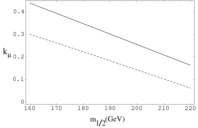
FIG. 1.: $k_{\mu}(\equiv Log_{10}[{{d_{\mu}^{e}}\over{1\times 10^{-23}{\rm ecm}}}])$ is plotted against $m_{1/2}$ for tan$\beta$=3 for case (i). The solid line is for $m_{0}=160$ GeV and the dotted line is for $m_{0}=170$. The other inputs are described in the text.

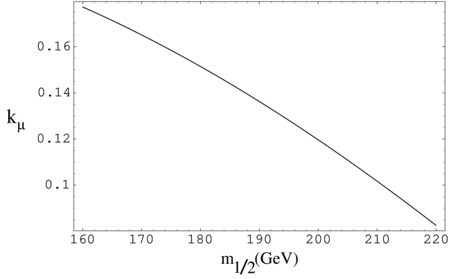
FIG. 2.: $k_{\mu}(\equiv Log_{10}[{{d_{\mu}^{e}}\over{1\times 10^{-23}{\rm ecm}}}])$ is plotted against $m_{1/2}$ for tan$\beta$=3 for case (ii). $m_{0}$ is 160 GeV. The other inputs are described in the text.

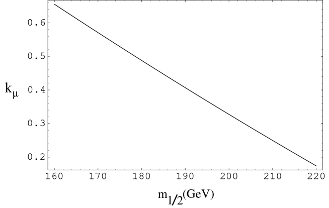
FIG. 3.: $k_{\mu}(\equiv Log_{10}[{{d_{\mu}^{e}}\over{1\times 10^{-23}{\rm ecm}}}])$ is plotted against $m_{1/2}$ for tan$\beta$=3 for the model with horizontal symmetry. $m_{0}$ is 85 GeV. The other inputs are described in the text.

REFERENCES

- [1] For reviews, see: S. Barr and W. Marciano, in CP violation, ed. by C. Jarlskog (World Scientific, 1988); W. Bernreuther and M. Suzuki, Rev. Mod. Phys. 63, 313 (1991).
- [2] I. S. Altarev et al., Phys. Lett. B 276, 242 (1992); K. F. Smith et al., Phys. Lett. B234, 191 (1990); P. G. Harris et al., Phys. Rev. Lett. 82, 904 (1999).
- [3] R. Golub and S. Lamoreaux, Proceedings of the Workshop on Baryon instability and Neutron-Anti-Neutron Oscillation, ed. Y. Kamyshkov, (1996).
- [4] E. Commins et al., Phys. Rev. A 50, 2960 (1994); K. Abdullah et al., Phys. Rev. Lett. 65, 2347 (1990).
- [5] J. Bailey et al., J. Phys. G4, 345 (1978).
- [6] Y. Semertzidis et al., E821 Collaboration at BNL, AGS Expression of Interest: Search for an Electric Dipole Moment of the Muon.
- [7] F. Hoogeveen, Nucl. Phys. B341, 322 (1990); I.B. Khriplovich and M. Pospelov, Sov. J. Nucl. Phys. 53, 638 (1991).
- [8] S. Barr and A. Zee, Phys. Rev. Lett. 65, 21 (1990); Erratum, 65, 2920 (1990).
- [9] V. Barger, A. Das and C. K. Kao, Phys. Rev. D55, 7099 (1997).
- [10] J. Ellis, S. Ferrara and D.V. Nanopoulos, Phys. Lett. B114, 231 (1982); J. Polchinski and M. Wise, Phys. Lett. 125B, 393 (1983); W. Buchmuller and D. Wyler, Phys. Lett. 121B, 321 (1983); F. Aguila, M. Gavela, J. Grifols and A. Mendez, Phys. Lett. B126, 71 (1983); ibid. B129, 473 (1983) (E); J.-M. Gerard, W. Grimus, D.V. Nanopoulos and A. Raychaudhuri, Nucl. Phys. B253, 93 (1985); E. Franco and M. Mangano, Phys. Lett. B135, 445 (1984); A. Sanda, Phys. Rev. D32, 2992 (1985); M. Dugan, B. Grinstein and L. Hall, Nucl. Phys. B255, 413 (1985); W. Bernreuther and M. Suzuki, Ref. [1].
- [11] P. Nath, Phys. Rev. Lett. 66, 2565 (1991); Y. Kizhukuri and N. Oshimo, Phys. Rev. D45, 1806 (1992); D46, 3025 (1992); R. Garisto and J. Wells, Phys. Rev. D55, 611 (1997).
- [12] T. Ibrahim and P. Nath, Phys. Lett. B418, 98 (1998); Phys. Rev. D57, 478 (1998); Phys. Rev. D58, 111301 (1998);
- [13] T. Falk and K. Olive, Phys. Lett. B439, 71 (1998); S. Barr and S. Khalil, Phys. Rev. D61, 035005 (2000); T. Falk, K. Olive, M. Pospelov and R. Roiban, Nucl. Phys. B560, 3 (1999); M. Brhlik, G. Good, and G. Kane, Phys. Rev. D 59, 115004 (1999); A. Bartl, T. Gajdosik, W. Porod, P. Stockinger and H. Stremnitzer, Phys. Rev.D60, 073003 (1999); S. Pokorski, J. Rosiek and C. A. Savoy, Nucl. Phys. B570, 81 (2000), E. Accomando, R. Arnowitt and B. Dutta, Phys. Rev. D61, 115003 (2000).
- [14] The Super-Kamiokande Collaboration, Phys. Rev. Lett. 81, 1562 (1998).
- [15] J.C. Pati and A. Salam, Phys. Rev. D 10, 275 (1974); R.N. Mohapatra and J.C. Pati, Phys. Rev. D11, 566, 2558 (1975); G. Senjanović and R.N. Mohapatra, Phys. Rev. D12, 1502 (1975).
- [16] M. Gell-Mann, P. Rammond and R. Slansky, in Supergravity, eds. D. Freedman et al. (North-Holland, Amsterdam, 1980); T. Yanagida, in Proc. KEK workshop, 1979 (unpublished); R.N. Mohapatra and G. Senjanović, Phys. Rev. Lett. 44, 912 (1980).
- [17] R.N. Mohapatra and A. Rasin, Phys. Rev. D 54, 5835 (1996).
- [18] K.S. Babu, B. Dutta and R.N. Mohapatra, Phys. Rev. D 60, 095004 (1999); ibid D61, 091701R (2000).
- [19] L. Hall, V. Kostelecky and S. Raby, Nucl. Phys. B267, 415, (1986); F. Gabbiani and A. Masiero, Nucl. Phys. B322, 235 (1989); N. Polonsky and A. Pomarol, Phys. Rev. Lett. 73, 2292 (1994); R. Barbieri, L. Hall and A. Strumia, Nucl. Phys. B445, 219 (1995); T.V. Duong, B. Dutta and E. Keith, Phys. Lett. B378, 128 (1996); J. Hisano and D. Nomura, Phys. Rev. D59, 116005 (1999).
- [20] K.S. Babu, B. Dutta and R. N. Mohapatra, hep-ph/9904366, Phys. Lett. 458, 93 (1999).
- [21] C. Hamzaoui, M. Pospelov and M. Toharia, Phys. Rev. D59, 095005 (1999).
- [22] K.S. Babu and S.M. Barr, Phys. Rev. Lett. 72, 2831 (1994). G. Eyal and Y. Nir, Nucl. Phys. B528, 21 (1998).
- [23] K.S. Babu, B. Dutta and R.N. Mohapatra, work in progress.
- [24] D. Chang, R.N. Mohapatra and M.K. Parida, Phys. Rev. Lett. 52, 1072 (1984).
- [25] C. Aulakh, A. Melfo and G.Senjanović, Phys. Rev. D57, 4174 (1998); Z. Chacko and R. N. Mohapatra, Phys. Rev. D 58, 015001 (1998).
- [26] C. Aulakh et al. Ref.[25].
- [27] ALEPH Collaboration, ALEPH contribution to the 2000 winter conference, ALEPH-2000-012, Conf-2000-009.
- [28] K.S. Babu and R.N. Mohapatra, Phys. Rev. Lett. 83, 2522 (1999).
- [29] J. Grifolis and A. Mendez, Phys. Rev. D26, 1809 (1982); J. Ellis, J. Hagelin and D.V. Nanopoulos, Phys. Lett. B116, 283 (1982); R. Barbieri and L. Maiani, Phys. Lett. B117, 203 (1982); D. Kosower, L. Krauss and N. Sakai, Phys. Lett. B133, 305 (1983); T. Yuan, R. Arnowitt, A. Chamseddine and P. Nath, Z. Phys. C26, 407 (1984); J. Lopez, D. Nanopoulos and X. Wang, Phys. Rev. D49, 366 (1994).
- [30] U. Chattopadhyay and P. Nath, Phys. Rev. D53, 1648 (1996).
- [31] M. Carena, G. Giudice and C. Wagner, Phys. Lett. B390, 234 (1997).
- [32] T. Moroi, Phys. Rev. D53, 6565 (1996); F. Borzumati, G. Farrar and N. Polonsky, Nucl. Phys. B555, 53 (1999), G-C. Cho, K. Hagiwara and M. Hayakawa, hep-ph/0001229.