UCLA-00-TEP-20

UM-TH-00-09

June 2000

Reduction and evaluation of two-loop graphs with arbitrary masses
Adrian Ghinculov^a and York-Peng Yao^b

^aDepartment of Physics and Astronomy, UCLA,
Los Angeles, California 90095-1547, USA
^bRandall Laboratory of Physics, University of Michigan,
Ann Arbor, Michigan 48109-1120, USA

We describe a general analytic-numerical reduction scheme for evaluating any two-loop diagrams with general kinematics and general renormalizable interactions, whereby ten special functions form a complete set after tensor reduction. We discuss the symmetrical analytic structure of these special functions in their integral representation, which allows for optimized numerical integration. The process $Z\to b\bar{b}$ is used for illustration, for which we evaluate all the three-point, non-factorizable $g^{2}\alpha_{s}$ mixed electroweak-QCD graphs, which depend on the top quark mass. The isolation of infrared singularities is detailed, and numerical results are given for all two-loop three-point graphs involved in this process.

Abstract

We describe a general analytic-numerical reduction scheme for evaluating any two-loop diagrams with general kinematics and general renormalizable interactions, whereby ten special functions form a complete set after tensor reduction. We discuss the symmetrical analytic structure of these special functions in their integral representation, which allows for optimized numerical integration. The process $Z\to b\bar{b}$ is used for illustration, for which we evaluate all the three-point, non-factorizable $g^{2}\alpha_{s}$ mixed electroweak-QCD graphs, which depend on the top quark mass. The isolation of infrared singularities is detailed, and numerical results are given for all two-loop three-point graphs involved in this process.

1 Introduction

The success of the perturbative aspect of the Standard Model is truly impressive, the theory being now tested at higher than one-loop accuracy. It is natural that over the past years various methods have been proposed to calculate higher loop graphs. Beyond one loop, there are situations in which one can neglect internal masses, or exploit the kinematics to evaluate amplitudes analytically at some special point where the Feynman diagrams become simpler. These special situations, while ingenious, cover only certain classes of physical processes.

There have been attempts to formulate solutions for two-loop Feynman diagrams, which ideally should be as general as the one-loop solutions are. For the massless case a lot of progress has been reached recently [1]. On the other hand, for the general massive case, it has become clear that some numerical treatment appears unavoidable because of the complexity of the scalar integrals involved.

In refs. [2, 3] a reduction scheme was found for treating massive self-energy diagrams at two-loop, with the resulting master scalar integrals being evaluated numerically.

In ref. [4] we investigated the problem of a general massive two-loop algorithm, which would deal with multi-leg diagrams as well. Once we subscribe to a semi-numerical approach, some demands must be made, which are based on the generality, the universality, the effectiveness and the accuracy that a particular formalism engenders. We have shown that for any external kinematics and internal masses, we can reduce every two-loop amplitude for a process due to any renormalizable interactions into a set of ten scalar integrals and their derivatives.

It is not hard to see how a result like this is obtained if we consider first a scalar theory with trivial interactions [5]. Then, there would be two internal momenta, $p$ and $q$, and by the use of Feynman parameters to combine sets of denominators in which either $p$ or $q$ or $p+q$ runs through, and to make shifts in $p$ and $q$, we have an integrand proportional to

$$1\over[(p+k)^{2}+m_{1}^{2}]^{\alpha_{1}}(q^{2}+m_{2}^{2})^{\alpha_{2}}[(p+q)^{2}+m_{3}^{2}]^{\alpha_{3}}$$ (1)

in which a four-vector $k$ is left over, which is a linear function of the external momenta and Feynman parameters. The “masses” $m_{1,2,3}^{2}$ are functions of external momenta, internal masses and Feynman parameters. These are to be integrated over $p$, $q$ and a set of Feynman parameters. By partial differentiating with respect to $m_{1,2,3}^{2}$, there is in principle only one basic function arising from $\alpha_{1}=\alpha_{2}=\alpha_{2}=1$ we need to know, although for convenience one may add $\alpha_{1}=2,\alpha_{2}=\alpha_{3}=1.$ It is clear that different interactions and different graphs will give different polynomials of Feynman parameters to the numerators, and also different $k$ and $m_{1,2,3}^{2}$. An extension of this construction to tensor integrals will give us the main result mentioned earlier.

In the following section, we discuss the steps and arguments needed to perform a tensorial decomposition. We show that there is a small set of basic functions which are needed, which have simple, one-dimensional integral representations. Their analytic structure is easy to see, and therefore the integration contour can be extended into the complex plane and optimized for rapid numerical convergence. In Section 3, we shall give a detailed exposition of the numerical techniques involved.

Given that two-point functions are usually simpler to calculate, many calculations existing in the literature used unitarity cuts of self-energies to calculate lower loop-order inclusive decay rates. We would like to stress that, given a process, our formalism allows us to calculate the amplitudes individually, as opposed to using unitarity cuts. As an immediate consequence, it becomes possible to obtain rates for exclusive processes, without the need to integrate over the whole final-state phase space.

In section 4, for illustration, we discuss in detail the application of our method to the important physical process $Z\to b\bar{b}$.

2 Analytical reduction

2.1 Relation with sunset-type integrals

The starting point of calculating a massive two-loop diagram is to express it in terms of integrals of a standard type. Topologically, any generic two-loop diagram can be represented in the form shown in figure 1. By introducing a set of Feynman parameters $X$ to combine all propagators which have the same loop integration momentum $p$, $q$, or $r=p+q$, the graph can always be represented as an integral over a sunset-type two-loop integral. This is illustrated in figure 1. All dependence on the external momenta $k_{i}$ and internal masses $m_{i}$ is now contained in the variables $m_{1}^{2}$, $m_{2}^{2}$, $m_{3}^{2}$, and $k$, which also depend on the set of Feynman parameters $X$.

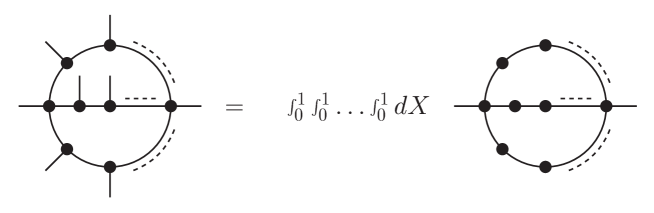
Figure 1: Expressing generic massive two-loop Feynman diagrams as integrals over sunset-type functions.

The original Feynman diagram is written at this point as an integral over tensor functions of the following type (all momenta are rotated into Euclidean):

$$\int d^{n}p\,d^{n}q\,\frac{p^{\mu_{1}}\ldots p^{\mu_{i}}q^{\mu_{i+1}}\ldots q^{\mu_{j}}}{[(p+k)^{2}+m_{1}^{2}]^{\alpha_{1}}\,(q^{2}+m_{2}^{2})^{\alpha_{2}}\,(r^{2}+m_{3}^{2})^{\alpha_{3}}}~{}~{}.$$ (2)

By casting the graph in this form, our strategy is to develop a uniform treatment of all possible sunset-type functions which can be generated from generic two-loop Feynman graphs. The further tensor reduction and decomposition into standard scalar functions is done by using standard formulae common for all diagrams. Therefore it can be automatized in the form of an algebraic manipulation program.

At the end, the remaining integral over the Feynman parameters $X$, represented in figure 1, is performed numerically.

2.2 Tensor reduction

Tensor integrals of the type in eqn. 2 need to be decomposed into scalar integrals. By Lorentz covariance, this two-loop integral is a tensor constructed from the external momentum $k^{\mu}$ and the metric tensor $g^{\mu\nu}$. Given that, one way of obtaining the tensor decomposition would be to write down all tensor structures allowed by the symmetry of the integral, use appropriate projectors, and solve the resulting equations.

Another way to do this is by decomposing the loop momenta $p$ and $q$ into components parallel and orthogonal to the external momentum $k^{\mu}$:

$$p_{\perp}^{\mu}=p^{\mu}-\frac{p\cdot k}{k^{2}}k^{\mu}~{}~{},~{}~{}q_{\perp}^{\mu}=q^{\mu}-\frac{q\cdot k}{k^{2}}k^{\mu}~{}~{}.$$ (3)

After this decomposition, the tensor decomposition is obtained by noticing that the functions with an odd number of transverse loop momenta $p_{\perp}^{\mu}$ and $q_{\perp}^{\mu}$ vanish, while the even functions are transverse to $k^{\mu}$ [4]. In ref. [4] we have shown that the resulting scalar coefficients of the tensor decomposition are integrals of the following form:

$$\tilde{\cal P}^{a\,b}_{\alpha_{1}\,\alpha_{2}\,\alpha_{3}}(m_{1},m_{2},m_{3};k^{2})=\int d^{n}p\,d^{n}q\,\frac{(p\cdot k)^{a}(q\cdot k)^{b}}{[(p+k)^{2}+m_{1}^{2}]^{\alpha_{1}}\,(q^{2}+m_{2}^{2})^{\alpha_{2}}\,(r^{2}+m_{3}^{2})^{\alpha_{3}}}~{}~{}.$$ (4)

We give in the following the tensor decompositions for all tensor integrals of the type of eq. 2 of rank 1, 2, and 3:

$$\frac{1}{[211]} = {{}_{1}A_{1}}~{}~{}~{}~{}~{}~{}~{}~{}~{}~{}~{}~{}~{}~{}~{}~{}~{}~{},~{}\frac{p^{\mu}}{[211]}=k^{\mu}{{}_{2}A_{1}}~{}~{}~{}~{}~{}~{}~{}~{}~{}~{}~{}~{}~{}~{},~{}\frac{q^{\mu}}{[211]}=k^{\mu}{{}_{3}A_{1}}$$

$$\frac{p^{\mu}p^{\nu}}{[211]} = \tau^{\mu\nu}{{}_{4}A_{1}}+g^{\mu\nu}{{}_{4}A_{2}}~{},~{}\frac{p^{\mu}q^{\nu}}{[211]}=\tau^{\mu\nu}{{}_{5}A_{1}}+g^{\mu\nu}{{}_{5}A_{2}}~{},~{}\frac{q^{\mu}q^{\nu}}{[211]}=\tau^{\mu\nu}{{}_{6}A_{1}}+g^{\mu\nu}{{}_{6}A_{2}}$$

$$\frac{p^{\mu}p^{\nu}p^{\lambda}}{[211]} = (\tau^{\mu\nu}k^{\lambda}+\tau^{\mu\lambda}k^{\nu}+\tau^{\nu\lambda}k^{\mu}){{}_{7}A_{1}}+(g^{\mu\nu}k^{\lambda}+g^{\mu\lambda}k^{\nu}+g^{\nu\lambda}k^{\mu}){{}_{7}A_{2}}$$

$$\frac{q^{\mu}p^{\nu}p^{\lambda}}{[211]} = (\tau^{\mu\nu}k^{\lambda}+\tau^{\mu\lambda}k^{\nu}+\tau^{\nu\lambda}k^{\mu}){{}_{8}A_{1}}+(g^{\mu\nu}k^{\lambda}+g^{\mu\lambda}k^{\nu}+g^{\nu\lambda}k^{\mu}){{}_{8}A_{2}}$$

$$\frac{p^{\mu}q^{\nu}q^{\lambda}}{[211]} = (\tau^{\mu\nu}k^{\lambda}+\tau^{\mu\lambda}k^{\nu}+\tau^{\nu\lambda}k^{\mu}){{}_{9}A_{1}}+(g^{\mu\nu}k^{\lambda}+g^{\mu\lambda}k^{\nu}+g^{\nu\lambda}k^{\mu}){{}_{9}A_{2}}$$

$$\;\;\;\;\;\;\;\;\;\;\;\;\;\;\;\;\;\;\;\;\;\;\;\;\;\;\;\;\;\;\;\;\;\;\;\;\;\;\;\;\;\;\;+(g^{\mu\nu}k^{\lambda}+g^{\mu\lambda}k^{\nu}-2g^{\nu\lambda}k^{\mu}){{}_{9}A_{3}}$$

$$\frac{q^{\mu}q^{\nu}q^{\lambda}}{[211]} = (\tau^{\mu\nu}k^{\lambda}+\tau^{\mu\lambda}k^{\nu}+\tau^{\nu\lambda}k^{\mu}){{}_{10}A_{1}}+(g^{\mu\nu}k^{\lambda}+g^{\mu\lambda}k^{\nu}+g^{\nu\lambda}k^{\mu}){{}_{10}A_{2}}$$

Tensor decompositions for more than three Lorentz indices are derived in a similar way. In the formulae above, a loop integration $\int d^{n}p\;d^{n}q$ is understood, and we used the following notations:

$$[211]=[(p+k)^{2}+m_{1}^{2}]^{2}\,(q^{2}+m_{2}^{2})\,(r^{2}+m_{3}^{2})~{}~{}~{},~{}~{}~{}\tau^{\mu\nu}=g^{\mu\nu}-\frac{k^{\mu}k^{\nu}}{k^{2}}$$ (5)

and:

$${}_{1}A_{1} = {\cal H}_{1}~{}~{}~{}~{}~{}~{}~{}~{}~{}~{}~{}~{}~{}~{}~{}~{}~{}~{}~{}~{}~{}~{}~{}~{}~{},~{}~{}~{}~{}~{}~{}~{}_{2}A_{1}=\frac{1}{k^{2}}{\cal H}_{2}~{}~{}~{}~{}~{}~{}~{}~{}~{}~{}~{}~{}~{},~{}~{}~{}_{3}A_{1}=\frac{1}{k^{2}}{\cal H}_{3}$$

$${}_{4}A_{1} = -\frac{1}{k^{2}}\frac{n}{n-1}{\cal H}_{4}~{}~{}~{}~{}~{}~{}~{}~{}~{}~{}~{}~{},~{}~{}~{}~{}~{}~{}_{4}A_{2}=\frac{1}{k^{2}}\tilde{{\cal P}}^{20}_{211}$$

$${}_{5}A_{1} = -\frac{1}{k^{2}}\frac{n}{n-1}{\cal H}_{5}~{}~{}~{}~{}~{}~{}~{}~{}~{}~{}~{}~{},~{}~{}~{}~{}~{}~{}_{5}A_{2}=\frac{1}{k^{2}}\tilde{{\cal P}}^{11}_{211}$$

$${}_{6}A_{1} = -\frac{1}{k^{2}}\frac{n}{n-1}{\cal H}_{6}~{}~{}~{}~{}~{}~{}~{}~{}~{}~{}~{}~{},~{}~{}~{}~{}~{}~{}_{6}A_{2}=\frac{1}{k^{2}}\tilde{{\cal P}}^{02}_{211}$$

$${}_{7}A_{1} = -\left(\frac{1}{k^{2}}\right)^{2}\frac{n+2}{3(n-1)}{\cal H}_{7}~{}~{},~{}~{}~{}~{}~{}~{}_{7}A_{2}=\left(\frac{1}{k^{2}}\right)^{2}\frac{1}{3}\tilde{{\cal P}}^{30}_{211}$$

$${}_{8}A_{1} = -\left(\frac{1}{k^{2}}\right)^{2}\frac{n+2}{3(n-1)}{\cal H}_{8}~{}~{},~{}~{}~{}~{}~{}~{}_{8}A_{2}=\left(\frac{1}{k^{2}}\right)^{2}\frac{1}{3}\tilde{{\cal P}}^{21}_{211}$$

$${}_{9}A_{1} = -\left(\frac{1}{k^{2}}\right)^{2}\frac{n+2}{3(n-1)}{\cal H}_{9}~{}~{},~{}~{}~{}~{}~{}~{}_{9}A_{2}=\left(\frac{1}{k^{2}}\right)^{2}\frac{1}{3}\tilde{{\cal P}}^{12}_{211}$$

$${}_{9}A_{3} = \frac{1}{k^{2}}\frac{1}{3}\left[\tilde{{\cal P}}^{11}_{211}+\tilde{{\cal P}}^{02}_{211}-\frac{n}{n-1}({\cal H}_{5}+{\cal H}_{6})\right]$$

$${}_{10}A_{1} = -\left(\frac{1}{k^{2}}\right)^{2}\frac{n+2}{3(n-1)}{\cal H}_{10}~{}~{},~{}~{}~{}~{}_{10}A_{2}=\left(\frac{1}{k^{2}}\right)^{2}\frac{1}{3}\tilde{{\cal P}}^{03}_{211}$$

In the expressions above, we introduced a set of ten scalar integrals ${\cal H}_{i}$, which are related to the $\tilde{{\cal P}}^{ab}_{211}$ functions, and are defined as follows:

$${\cal H}_{1} = \int d^{n}p\,d^{n}q\,\frac{1}{[(p+k)^{2}+m_{1}^{2}]^{2}\,(q^{2}+m_{2}^{2})\,(r^{2}+m_{3}^{2})}$$

$${\cal H}_{2} = \int d^{n}p\,d^{n}q\,\frac{p\cdot k}{[(p+k)^{2}+m_{1}^{2}]^{2}\,(q^{2}+m_{2}^{2})\,(r^{2}+m_{3}^{2})}$$

$${\cal H}_{3} = \int d^{n}p\,d^{n}q\,\frac{q\cdot k}{[(p+k)^{2}+m_{1}^{2}]^{2}\,(q^{2}+m_{2}^{2})\,(r^{2}+m_{3}^{2})}$$

$${\cal H}_{4} = \int d^{n}p\,d^{n}q\,\frac{(p\cdot k)^{2}-\frac{1}{n}k^{2}p^{2}}{[(p+k)^{2}+m_{1}^{2}]^{2}\,(q^{2}+m_{2}^{2})\,(r^{2}+m_{3}^{2})}$$

$${\cal H}_{5} = \int d^{n}p\,d^{n}q\,\frac{(p\cdot k)(q\cdot k)-\frac{1}{n}k^{2}(q\cdot p)}{[(p+k)^{2}+m_{1}^{2}]^{2}\,(q^{2}+m_{2}^{2})\,(r^{2}+m_{3}^{2})}$$

$${\cal H}_{6} = \int d^{n}p\,d^{n}q\,\frac{(q\cdot k)^{2}-\frac{1}{n}k^{2}q^{2}}{[(p+k)^{2}+m_{1}^{2}]^{2}\,(q^{2}+m_{2}^{2})\,(r^{2}+m_{3}^{2})}$$

$${\cal H}_{7} = \int d^{n}p\,d^{n}q\,\frac{(p\cdot k)^{3}-\frac{3}{n+2}k^{2}p^{2}(p\cdot k)}{[(p+k)^{2}+m_{1}^{2}]^{2}\,(q^{2}+m_{2}^{2})\,(r^{2}+m_{3}^{2})}$$

$${\cal H}_{8} = \int d^{n}p\,d^{n}q\,\frac{(p\cdot k)^{2}(q\cdot k)-\frac{3}{n+2}k^{2}p^{2}(q\cdot k)}{[(p+k)^{2}+m_{1}^{2}]^{2}\,(q^{2}+m_{2}^{2})\,(r^{2}+m_{3}^{2})}$$

$${\cal H}_{9} = \int d^{n}p\,d^{n}q\,\frac{(p\cdot k)(q\cdot k)^{2}-\frac{1}{n+2}k^{2}[2(p\cdot q)(q\cdot k)+q^{2}(p\cdot k)]}{[(p+k)^{2}+m_{1}^{2}]^{2}\,(q^{2}+m_{2}^{2})\,(r^{2}+m_{3}^{2})}$$

$${\cal H}_{10} = \int d^{n}p\,d^{n}q\,\frac{(q\cdot k)^{3}-\frac{3}{n+2}k^{2}q^{2}(q\cdot k)}{[(p+k)^{2}+m_{1}^{2}]^{2}\,(q^{2}+m_{2}^{2})\,(r^{2}+m_{3}^{2})}$$ (6)

As it can be seen in eqs. 5, these scalar functions appear naturally in the tensorial decomposition. As discussed in the following section, the functions ${\cal H}_{i}$ are only logarithmically divergent in the ultraviolet. Because of this, they have very simple integral representations which can be used for numerical computation. Once a way of calculating the special functions ${\cal H}_{i}$ is available, the $\tilde{\cal P}^{ab}_{2\,1\,1}$ functions can easily be recovered by partial fractioning eqns. 6. The partial fractioning generates essentially trivial products of one-loop tadpoles. The conversion formulae are given in Appendix A.

2.3 Integral representation of the ${\cal H}_{i}$ functions

Because the ultraviolet behaviour of the functions ${\cal H}_{i}$ is logarithmic, fairly simple and symmetric integral representations can be found [4]:

$${\cal H}_{1} = \pi^{4}\left[\frac{2}{\epsilon^{2}}-\frac{1}{\epsilon}(1-2\gamma_{m_{1}})-\frac{1}{2}+\frac{\pi^{2}}{12}-\gamma_{m_{1}}+\gamma_{m_{1}}^{2}+h_{1}\right]$$

$${\cal H}_{2} = \pi^{4}k^{2}\left[-\frac{2}{\epsilon^{2}}+\frac{1}{\epsilon}(\frac{1}{2}-2\gamma_{m_{1}})+\frac{13}{8}-\frac{\pi^{2}}{12}+\frac{\gamma_{m_{1}}}{2}-\gamma_{m_{1}}^{2}-h_{2}\right]$$

$${\cal H}_{3} = \pi^{4}k^{2}\left[\frac{1}{\epsilon^{2}}-\frac{1}{\epsilon}(\frac{1}{4}-\gamma_{m_{1}})-\frac{13}{16}+\frac{\pi^{2}}{24}-\frac{\gamma_{m_{1}}}{4}+\frac{\gamma_{m_{1}}^{2}}{2}+h_{3}\right]$$

$${\cal H}_{4} = \pi^{4}(k^{2})^{2}\left[\frac{3}{2\epsilon^{2}}+\frac{1}{\epsilon}\frac{3\gamma_{m_{1}}}{2}-\frac{175}{96}+\frac{\pi^{2}}{16}+\frac{3\gamma_{m_{1}}^{2}}{4}+\frac{3}{4}h_{4}\right]$$

$${\cal H}_{5} = \pi^{4}(k^{2})^{2}\left[-\frac{3}{4\epsilon^{2}}-\frac{1}{\epsilon}\frac{3\gamma_{m_{1}}}{4}+\frac{175}{192}-\frac{\pi^{2}}{32}-\frac{3\gamma_{m_{1}}^{2}}{8}-\frac{3}{4}h_{5}\right]$$

$${\cal H}_{6} = \pi^{4}(k^{2})^{2}\left[\frac{1}{2\epsilon^{2}}-\frac{1}{\epsilon}(\frac{1}{24}-\frac{\gamma_{m_{1}}}{2})-\frac{19}{32}+\frac{\pi^{2}}{48}-\frac{\gamma_{m_{1}}}{24}+\frac{\gamma_{m_{1}}^{2}}{4}+\frac{3}{4}h_{6}\right]$$

$${\cal H}_{7} = \pi^{4}(k^{2})^{3}\left[-\frac{1}{\epsilon^{2}}-\frac{1}{\epsilon}(\frac{5}{24}+\gamma_{m_{1}})+\frac{287}{192}-\frac{\pi^{2}}{24}-\frac{5\gamma_{m_{1}}}{24}-\frac{\gamma_{m_{1}}^{2}}{2}-\frac{1}{2}h_{7}\right]$$

$${\cal H}_{8} = \pi^{4}(k^{2})^{3}\left[\frac{1}{2\epsilon^{2}}+\frac{1}{\epsilon}(\frac{5}{48}+\frac{\gamma_{m_{1}}}{2})-\frac{287}{384}+\frac{\pi^{2}}{48}+\frac{5\gamma_{m_{1}}}{48}+\frac{\gamma_{m_{1}}^{2}}{4}+\frac{1}{2}h_{8}\right]$$

$${\cal H}_{9} = \pi^{4}(k^{2})^{3}\left[-\frac{1}{3\epsilon^{2}}-\frac{1}{\epsilon}(\frac{1}{24}+\frac{\gamma_{m_{1}}}{3})+\frac{95}{192}-\frac{\pi^{2}}{72}-\frac{\gamma_{m_{1}}}{24}-\frac{\gamma_{m_{1}}^{2}}{6}-\frac{1}{2}h_{9}\right]$$

$${\cal H}_{10} = \pi^{4}(k^{2})^{3}\left[\frac{1}{4\epsilon^{2}}+\frac{1}{\epsilon}(\frac{1}{96}+\frac{\gamma_{m_{1}}}{4})-\frac{283}{768}+\frac{\pi^{2}}{96}+\frac{\gamma_{m_{1}}}{96}+\frac{\gamma_{m_{1}}^{2}}{8}+\frac{1}{2}h_{10}\right]\;\;.$$ (7)

Here, $n=4+\epsilon$ is the space-time dimension, and $\gamma_{m}=\gamma+\log(\pi m^{2}/\mu_{1}^{2})$ ($\gamma$ is the Euler constant, and $\mu_{1}$ is the ’t Hooft mass). The special functions $h_{i}$ which appear in the formulae above are the finite part in the $1/\epsilon$ expansion of ${\cal H}_{i}$. They are defined by the following integral representations. Except for special values of their arguments, they cannot be further integrated into well-studied functions, such as the familiar polylogarithms, and as such, our strategy is to evaluate them numerically directly from their integral representations:

$$h_{1}(m_{1},m_{2},m_{3};k^{2}) = \int_{0}^{1}dx\,\tilde{g}(x)$$

$$h_{2}(m_{1},m_{2},m_{3};k^{2}) = \int_{0}^{1}dx\,[\tilde{g}(x)+\tilde{f_{1}}(x)]$$

$$h_{3}(m_{1},m_{2},m_{3};k^{2}) = \int_{0}^{1}dx\,[\tilde{g}(x)+\tilde{f_{1}}(x)]\,(1-x)$$

$$h_{4}(m_{1},m_{2},m_{3};k^{2}) = \int_{0}^{1}dx\,[\tilde{g}(x)+\tilde{f_{1}}(x)+\tilde{f_{2}}(x)]$$

$$h_{5}(m_{1},m_{2},m_{3};k^{2}) = \int_{0}^{1}dx\,[\tilde{g}(x)+\tilde{f_{1}}(x)+\tilde{f_{2}}(x)]\,(1-x)$$

$$h_{6}(m_{1},m_{2},m_{3};k^{2}) = \int_{0}^{1}dx\,[\tilde{g}(x)+\tilde{f_{1}}(x)+\tilde{f_{2}}(x)]\,(1-x)^{2}$$

$$h_{7}(m_{1},m_{2},m_{3};k^{2}) = \int_{0}^{1}dx\,[\tilde{g}(x)+\tilde{f_{1}}(x)+\tilde{f_{2}}(x)+\tilde{f_{3}}(x)]$$

$$h_{8}(m_{1},m_{2},m_{3};k^{2}) = \int_{0}^{1}dx\,[\tilde{g}(x)+\tilde{f_{1}}(x)+\tilde{f_{2}}(x)+\tilde{f_{3}}(x)]\,(1-x)$$

$$h_{9}(m_{1},m_{2},m_{3};k^{2}) = \int_{0}^{1}dx\,[\tilde{g}(x)+\tilde{f_{1}}(x)+\tilde{f_{2}}(x)+\tilde{f_{3}}(x)]\,(1-x)^{2}$$

$$h_{10}(m_{1},m_{2},m_{3};k^{2}) = \int_{0}^{1}dx\,[\tilde{g}(x)+\tilde{f_{1}}(x)+\tilde{f_{2}}(x)+\tilde{f_{3}}(x)]\,(1-x)^{3}\;\;.$$ (8)

The four building blocks $\tilde{g}(x)$, $\tilde{f_{1}}(x)$, $\tilde{f_{2}}(x)$, and $\tilde{f_{3}}(x)$ of these one-dimensional integral representations are given in Appendix B.

2.4 Completeness of the $\{{\cal H}_{i}\}_{i=\overline{1,10}}$ special functions for renormalizable theories

The ten special functions ${\cal H}_{i}$ we introduced in the previous section, or, equivalently, their corresponding $\tilde{\cal P}^{ab}_{\alpha_{1}\alpha_{2}\alpha_{3}}$, are sufficient for treating all two-loop Feynman graphs which may be encountered in renormalizable theories.

To see this, it is useful to define the following auxiliary two-loop functions:

$${\cal P}^{a\,b}_{\alpha_{1}\,\alpha_{2}\,\alpha_{3}}(m_{1},m_{2},m_{3};k^{2})=\int d^{n}p\,d^{n}q\,\frac{(p\cdot k)^{a}(q\cdot k)^{b}}{(p^{2}+m_{1}^{2})^{\alpha_{1}}\,(q^{2}+m_{2}^{2})^{\alpha_{2}}\,[(r+k)^{2}+m_{3}^{2}]^{\alpha_{3}}}~{}~{}.$$ (9)

${\cal P}^{ab}_{\alpha_{1}\alpha_{2}\alpha_{3}}$ are trivially related to $\tilde{\cal P}^{ab}_{\alpha_{1}\alpha_{2}\alpha_{3}}$ by a simple redefinition of the loop momentum (see Appendix A). The only reason for introducing them is for simplifying the discussion of this section; some recursion relations can be written more compactly in terms of these scalar functions.

To prove our assertion that the set of ten $\{{\cal H}_{i}\}$ functions is sufficient for the case of renormalizable theories, we notice that not all functions ${\cal P}^{ab}_{\alpha_{1}\alpha_{2}\alpha_{3}}$ of various indices are independent. There are recursion relations which relate functions of different indices.

We will define the “degree” of a ${\cal P}^{ab}_{\alpha_{1}\alpha_{2}\alpha_{3}}$ function as $\alpha_{1}+\alpha_{2}+\alpha_{3}-a-b$. The degree can be increased by differentiating with respect to the mass variables:

$${\cal P}^{a\,b}_{\alpha_{1}+1\,\alpha_{2}\,\alpha_{3}}(m_{1},m_{2},m_{3};k^{2})=-\frac{1}{\alpha_{1}}\frac{\partial}{\partial m_{1}^{2}}{\cal P}^{a\,b}_{\alpha_{1}\,\alpha_{2}\,\alpha_{3}}(m_{1},m_{2},m_{3};k^{2})\;\;,$$ (10)

and similarly for $\alpha_{2}$ and $\alpha_{3}$.

Functions of the same degree are related by recursion relations obtained by differentiating with respect to the external momentum variable $k^{\mu}$:

$${\cal P}^{a+1\,b}_{\alpha_{1}+1\,\alpha_{2}\,\alpha_{3}} = \frac{1}{2\;\alpha_{1}}\left[2k^{2}\frac{\partial}{\partial k^{2}}-(a+b)\right]{\cal P}^{a\,b}_{\alpha_{1}\,\alpha_{2}\,\alpha_{3}}+\frac{ak^{2}}{2\alpha_{1}}{\cal P}^{a-1\,b}_{\alpha_{1}\,\alpha_{2}\,\alpha_{3}}$$

$${\cal P}^{a\,b+1}_{\alpha_{1}\,\alpha_{2}+1\,\alpha_{3}} = \frac{1}{2\;\alpha_{2}}\left[2k^{2}\frac{\partial}{\partial k^{2}}-(a+b)\right]{\cal P}^{a\,b}_{\alpha_{1}\,\alpha_{2}\,\alpha_{3}}+\frac{bk^{2}}{2\alpha_{2}}{\cal P}^{a\,b-1}_{\alpha_{1}\,\alpha_{2}\,\alpha_{3}}\;\;,$$ (11)

and

$$\left[2k^{2}\frac{\partial}{\partial k^{2}}-(a+b)\right]{\cal P}^{a\,b}_{\alpha_{1}\,\alpha_{2}\,\alpha_{3}}=-2\alpha_{3}\left[k^{2}{\cal P}^{a\,b}_{\alpha_{1}\,\alpha_{2}\,\alpha_{3}+1}+{\cal P}^{a+1\,b}_{\alpha_{1}\,\alpha_{2}\,\alpha_{3}+1}+{\cal P}^{a\,b+1}_{\alpha_{1}\,\alpha_{2}\,\alpha_{3}+1}\right]\;\;.$$ (12)

When calculating a specific process, it is thus possible to just focus on the lowest order ${\cal P}^{ab}_{\alpha_{1}\alpha_{2}\alpha_{3}}$ functions involved. All the other can be derived from these by differentiation, by using the relations above.

At the same time, in renormalizable theories, there is a lower bound on the possible degree of ${\cal P}^{ab}_{\alpha_{1}\alpha_{2}\alpha_{3}}$ functions involved in two-loop graphs, imposed by the dimension of the operators in the Lagrangian. The minimal degree is one, and is attained for instance by a two-loop diagram such as the one shown in figure 2. Additional external legs can at most increase the degree of the ${\cal P}^{ab}_{\alpha_{1}\alpha_{2}\alpha_{3}}$ functions involved.

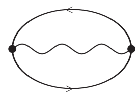
Figure 2: Two-loop diagram which involves ${\cal P}^{ab}_{\alpha_{1}\alpha_{2}\alpha_{3}}$ functions of minimal degree one. It consists of a fermion loop, a boson propagator, and non-derivative vertices.

Therefore, the most obvious choice of a basic set is the ${\cal P}^{ab}_{\alpha_{1}\alpha_{2}\alpha_{3}}$ functions with $\alpha_{1}=\alpha_{2}=\alpha_{3}=1$, $a+b=0,1,2$:

$$\begin{array}[]{llll}\mbox{degree}=3:&{\cal P}^{0\,0}_{1\,1\,1}&&\\ \mbox{degree}=2:&{\cal P}^{1\,0}_{1\,1\,1}&{\cal P}^{0\,1}_{1\,1\,1}&\\ \mbox{degree}=1:&{\cal P}^{2\,0}_{1\,1\,1}&{\cal P}^{1\,1}_{1\,1\,1}&{\cal P}^{0\,2}_{1\,1\,1}\par\end{array}$$ (13)

However, we prefer to use the functions with $\alpha_{1}=2$, $\alpha_{2}=\alpha_{3}=1$, $a+b=0,1,2,3$ instead:

$$\begin{array}[]{lllll}\mbox{degree}=4:&{\cal P}^{0\,0}_{2\,1\,1}&&&\\ \mbox{degree}=3:&{\cal P}^{1\,0}_{2\,1\,1}&{\cal P}^{0\,1}_{2\,1\,1}&&\\ \mbox{degree}=2:&{\cal P}^{2\,0}_{2\,1\,1}&{\cal P}^{1\,1}_{2\,1\,1}&{\cal P}^{0\,2}_{2\,1\,1}&\\ \mbox{degree}=1:&{\cal P}^{3\,0}_{2\,1\,1}&{\cal P}^{2\,1}_{2\,1\,1}&{\cal P}^{1\,2}_{2\,1\,1}&{\cal P}^{0\,3}_{2\,1\,1}\end{array}$$ (14)

It turns out that this equivalent set of functions has simpler integral representations than the functions of eqs. 13. When needed, the eqs. 13 functions can be derived from eqs. 14 by partial $p$:

$${\cal P}^{a\,b}_{\alpha_{1}\,\alpha_{2}\,\alpha_{3}} = -\frac{1}{n-(\alpha_{1}+\alpha_{2}+\alpha_{3})+(a+b)/2}\left\{\alpha_{1}m_{1}^{2}{\cal P}^{a\,b}_{\alpha_{1}+1\,\alpha_{2}\,\alpha_{3}}+\alpha_{2}m_{2}^{2}{\cal P}^{a\,b}_{\alpha_{1}\,\alpha_{2}+1\,\alpha_{3}}\right.$$ (15)

$$\left.\;\;\;\;\;\;\;\;\;\;\;\;\;\;\;\;\;+\alpha_{3}m_{3}^{2}{\cal P}^{a\,b}_{\alpha_{1}\,\alpha_{2}\,\alpha_{3}+1}-\frac{1}{2}\left[2k^{2}\frac{\partial}{\partial k^{2}}-(a+b)\right]{\cal P}^{a\,b}_{\alpha_{1}\,\alpha_{2}\,\alpha_{3}}\right\}\;\;,$$

Because the set of functions of eqs. 14 and the ten ${\cal H}_{i}$ functions differ essentially by simple, one-loop tadpole contributions given in Appendix A, this proves our assertion that the ten ${\cal H}_{i}$ functions are sufficient for treating renormalizable theories at two-loop.

We would like to stress that additional recursion relations and symmetries exist among this set of functions. An example of such a symmetry relation is given in eq. 16 of ref. [4], and additional ones may be present. Such relations can be used, in principle, for restraining the number of master functions involved. However, the set of ten ${\cal H}_{i}$ that we proposed has the advantage of having clean, symmetrical integral representations, where permutations of mass arguments are not involved, while symmetry relations obtained by loop momenta redefinitions often interchange the mass arguments. This simplicity is an advantage in practical calculations done by computer algebra, where a simpler algorithm may be preferable to a more complicated one which produces somewhat more compact results.

Thus, on general grounds, all tensor integrals ${\cal P}^{ab}_{\alpha_{1}\alpha_{2}\alpha_{3}}$ with $a+b\geq 4$ can be expressed by the standard set of ten functions via mass or momentum differentiation. The differentiations required can be carried out either by hand, or automatically, by using a computer algebra program such as Mathematica or Maple.

However, in practical calculations of Feynman graphs, before performing the tensor decomposition, it is advantageous to exploit all possible partial fractioning of the loop momenta, instead of resorting to recursion relations after the tensor decomposition. This can result in more compact results. This is in particular the case with the examples given in section 4. There, the calculation can be simplified by noticing that in the Feynman gauge, loop momenta $p$ and $q$ in the numerators come from fermion propagators, and there are no more than four of them. For those terms with four powers of $p$ and $q$, one can algebraically rearrange them, so that two of these powers will contract as $p^{2}$, $q^{2}$ or $p\cdot q$, and then perform partial fractioning of these terms, to reduce them into $\tilde{P}$ functions with $a+b\leq 3$.

3 Numerical integration

Once the tensor reduction is done analytically, the original Feynman diagram is expressed, according to figure 1, as an integral over the set of remaining Feynman parameters ${X}$. The integrand itself consists of a sum of $h_{i}$ special functions and possibly trivial functions such as logarithms and rational functions of the kinematic variables $m_{1}^{2}$, $m_{2}^{2}$, $m_{3}^{2}$, and $k^{2}$.

The $h_{i}$ functions themselves are given by the one-dimensional integral representations given in eqns. 8. Within our method, all these integration steps are performed numerically in general.

Therefore, it is natural to separate the numerical integration into two distinct steps: the routines to calculate the $h_{i}$ functions from their integral representations, and the final integration over the remaining Feynman parameters ${X}$.

When performing the numerical integration, special care is needed to make sure that the integration is performed on the physical sheet. Let us start with the integration of the $h_{i}$ functions.

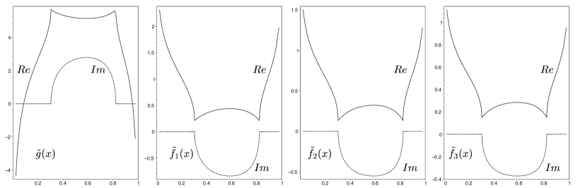
Figure 3: Typical behaviour of functions $\tilde{g}(x)$, $\tilde{f}_{1}(x)$, $\tilde{f}_{2}(x)$, $\tilde{f}_{3}(x)$ and of their derivatives as a function of the integration parameter $x$. The specific kinematic variables in these plots are above threshold, $-k^{2}>(m_{1}+m_{2}+m3)^{2}$, where an imaginary part is present.

In figure 3 we plot the functions $\tilde{g}(x)$ and $\tilde{f}_{i}(x)$ as a function of the integration parameter $x$. This is a typical behaviour above the threshold. At $x=0$ there is an integrable singularity of the logarithmic type, and similarly at $x=1$. By mass or momentum differentiation the integrable nature of these singularities in $x$ is not changed; this makes possible the treatment of more complicated topologies with additional external legs by using the same numerical approach. Along the integration path there are two branching points, between which the function acquires an imaginary part. The integration path must be chosen such as to reproduce correctly this imaginary part.

By continuing the integration parameter $x$ into the complex plane, we obtain a picture of the $h_{i}$ function’s integrand as shown in figure 4. It is clear that if the position of the two branching points is known, a correct integration path can be calculated automatically by the computer program. Finding the singularities involves some subtleties.

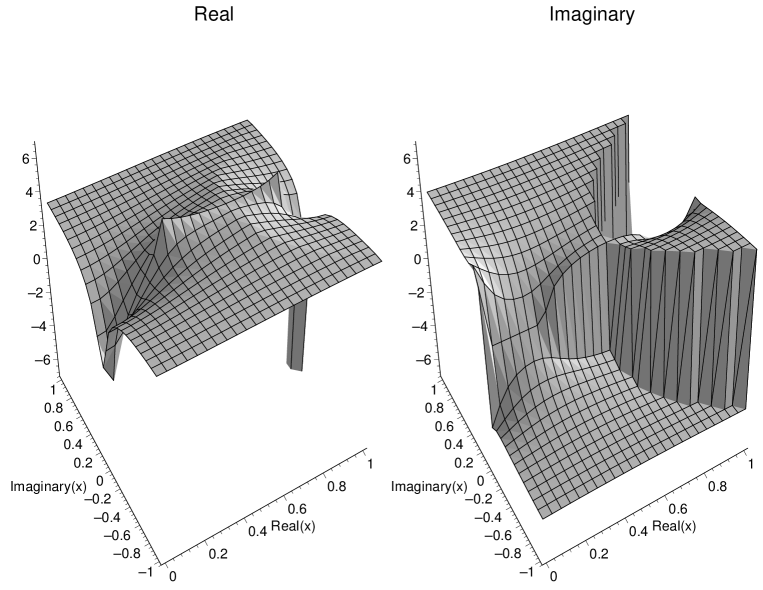
Figure 4: Typical behaviour of the functions $\tilde{g}(x)$, $\tilde{f}_{1}(x)$, $\tilde{f}_{2}(x)$, $\tilde{f}_{3}(x)$ and of their derivatives in the complex integration parameter $x$. The integration proceeds from $x=0$ to $x=1$.

Adopting the notations introduced in Appendix B, and inspecting the expressions of the functions $\tilde{g}(x)$, $\tilde{f}_{1}(x)$, $\tilde{f}_{2}(x)$ and $\tilde{f}_{3}(x)$ given there, the branching points we are looking for must be among the solutions of the equation:

$$\Delta\equiv(1+\kappa^{2}-\mu^{2})^{2}+4\kappa^{2}\mu^{2}-4i\kappa^{2}\eta=0~{}~{}.$$ (16)

There are four solutions:

$$x_{1,2} = \frac{1}{2\mu_{1}^{2}}\,[\,-a+b+\mu_{1}^{2}\pm\sqrt{(a-b-\mu_{1}^{2})^{2}-4b\mu_{1}^{2}}\,]$$

$$x_{3,4} = \frac{1}{2\mu_{2}^{2}}\,[\,-a+b+\mu_{2}^{2}\pm\sqrt{(a-b-\mu_{2}^{2})^{2}-4b\mu_{2}^{2}}\,]\;\;,$$

$$\mu_{1,2}^{2} = 1-\kappa^{2}\mp 2\sqrt{-\kappa^{2}}~{}~{}.$$ (17)

To establish which two of the four solutions are the branching points we are looking for, it is useful to note that the causality of the Green’s functions can be expressed in at least two equivalent ways, which ought to lead to the same prescription for the integration path. The causality condition is expressed by the $i\eta$ prescription in the Feynman propagator, which means to shift all masses in the propagators $m^{2}\rightarrow m^{2}-i\eta$. An equivalent way to impose causality is to calculate the Euclidian Green’s functions and to go afterwards to physical momenta, approaching the cut on the positive real axis from above. This amounts to shifting the external momentum $k^{2}\rightarrow k^{2}+i\eta$. These two prescriptions ought to be equivalent, and therefore have to fix the location of the physical singularities with respect to the real axis in the same way. For $x_{1}$ and $x_{2}$, at $-\kappa^{2}>1$ both prescriptions lead to the same change, and therefore these are the singularities of the $\tilde{g}$ and $\tilde{f}_{i}$ functions. For $x_{3}$ and $x_{4}$, the two prescriptions lead to opposite changes in the imaginary direction. Since causality fixes the location of the singularities of the Green’s function uniquely, $x_{3}$ and $x_{4}$ cannot correspond to real singularities of $\tilde{g}$ and $\tilde{f}_{i}$. Therefore $\tilde{g}$ and $\tilde{f}_{i}$ are analytical at these two points. The $\tilde{g}$ and $\tilde{f}_{i}$ functions themselves have only two branching points at $x_{1}$ and $x_{2}$, because the singularities at $x_{3}$ and $x_{4}$ are compensating among the four terms of $\tilde{g}$ in eq. 26. It is interesting to notice that the spurious solutions $x_{3}$ and $x_{4}$ correspond to the spurious, unphysical thresholds discussed in ref. [6] in the context of the relation of the scalar sunset diagram with a generalization of hypergeometric functions.

Once the positions of these two singularities are known, the computer program can automatically compute an integration path which avoids them. Because we are interested in a high accuracy and efficiency routine, we used an adaptive deterministic integration algorithm. Such integration routines are very accurate provided that the integrand is smooth enough. The integrand itself is, of course, an analytic function along the complex integration path, and to preserve its smoothness it is advantageous to define a smooth integration path as well. We use an integration path defined in terms of higher-order spline functions such that both the path and its Jacobian are smooth functions. A typical path is shown in figure 5.

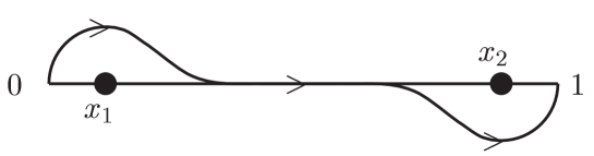
Figure 5: A typical shape for the complex integration path, defined in terms of higher order spline functions. Both the path and the Jacobian are smooth functions.

Along these lines, a fully automatic computer program can be written, which first identifies the singularities, then calculates a suitable complex integration path, and then performs the numerical integration to obtain the $h_{i}$ functions starting from their integral representations given in eqs. 8. By using adaptive integration routines, one typical evaluation of an $h_{i}$ function or of a derivative at eight digits takes of the order of 30 ms on a 600 MHz Pentium processor.

Figure 6: Plots of the ten special functions $h_{i}(m_{1}^{2},m_{2}^{2},m_{3}^{2};-k^{2})$ as a function of the external momentum variable $k^{2}$. The plots given here are for $m_{1}^{2}=m_{2}^{2}=m_{3}^{2}=1$.

In practical calculations of Feynman graphs, a number of mass or momentum derivatives of the functions $h_{i}$ become necessary. They can easily be obtained either by hand, or automatically, by computer algebra programs such as Mathematica or Maple.

The numerical integration over the remaining Feynman parameters ${X}$ is carried out along similar lines [5, 8, 9]. The dimensionality of this final integration depends on the topology of the diagram and on the number of legs.

With increasing complexity of the diagram, the methods we describe in this paper will still be applicable in principle, but in practice will result in larger integrands and a final numerical integration of higher dimension. Thus its applicability will be limited in practice by the available computing power and by the ability of handling potentially large expressions which result from the tensor reduction in an error free way.

4 Examples

4.1 Three-point two-loop diagrams contributing to $Z\rightarrow b\bar{b}$

Here we would like to illustrate by means of a concrete example how the algorithm described above works in practice. Examples involving two-point functions were given in ref. [8, 9]. Here, we treat all two-loop three-point diagrams which contribute to the important physical process $Z\rightarrow b\bar{b}$ at ${\cal O}(\alpha_{s}g^{2})$. The diagrams involved are shown in figure 7. In the complete calculation of this process, there are also self-energy type diagrams which contribute to the $b$ wave function renormalization. These two-point function graphs are simpler than the three-point graphs both analytically and numerically. Within our method, they were calculated in ref. [8]. The process $Z\rightarrow b\bar{b}$ at ${\cal O}(\alpha_{s}g^{2})$ at ${\cal O}(\alpha_{s}g^{2})$ was calculated by means of a mass expansion in ref. [7].

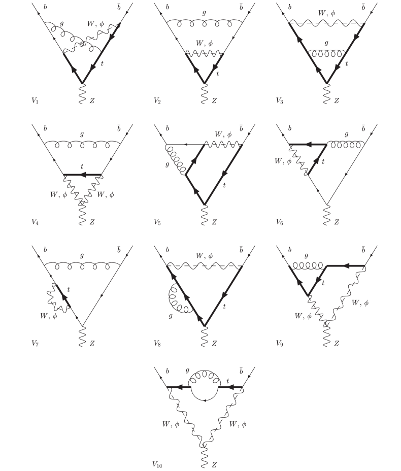
Figure 7: Two-loop three-point diagrams contributing to $Z\rightarrow b\bar{b}$ at ${\cal O}(\alpha_{s}g^{2})$.

4.2 Isolating the IR singularities

The two-loop methods we describe in this paper are intended primarily for the calculation of massive diagrams. However, sometimes massless particles are involved in a calculation and may lead to infrared singularities. We would like to stress that for purely massless calculations, such as QCD radiative corrections, more efficient methods are available already in the literature, which make use of the absence of masses [1]. It is often possible in the massless case to carry out the calculation completely analytically. The discussion in this section applies to cases where the main difficulty is related to the presence of several masses, while the infrared structure is relatively simple. Typical examples are the purely electroweak and the mixed electroweak-QCD radiative corrections, such as the $Z\rightarrow b\bar{b}$ at ${\cal O}(\alpha_{s}g^{2})$ process discussed here.

The diagrams $V_{2}$, $V_{4}$, $V_{6}$, and $V_{7}$ are infrared divergent. The most common treatment of IR divergencies uses dimensional regularization to separate both the UV and the IR singularities. In our approach however, this is not directly possible because in the expressions of eqs. 7 the $1/\epsilon$ expansion already separated the UV singularities, while the possible IR singularities are still contained in the integral representations of the finite parts $h_{i}$, with the intention of calculating these finite parts by numerical integration.

Therefore it is useful to separate first the infrared part of the two-loop diagrams in an analytically manageable form (one-loop diagrams in this case). The “real two-loop” calculation which is left after this separation is then free of infrared singularities. The analytical separation of infrared divergencies is performed by noticing that the IR behaviour of the two-loop diagrams comes essentially only from the loop integration over the gluon propagator. Then, the IR behaviour is left unchanged if the loop momentum on the propagator common to the two loop integrations ($r$) is being “frozen” to the loop momentum of the IR-finite loop. This analytical separation of the IR behaviour is given in figure 8 for all IR divergent two-loop diagrams involved in this process.

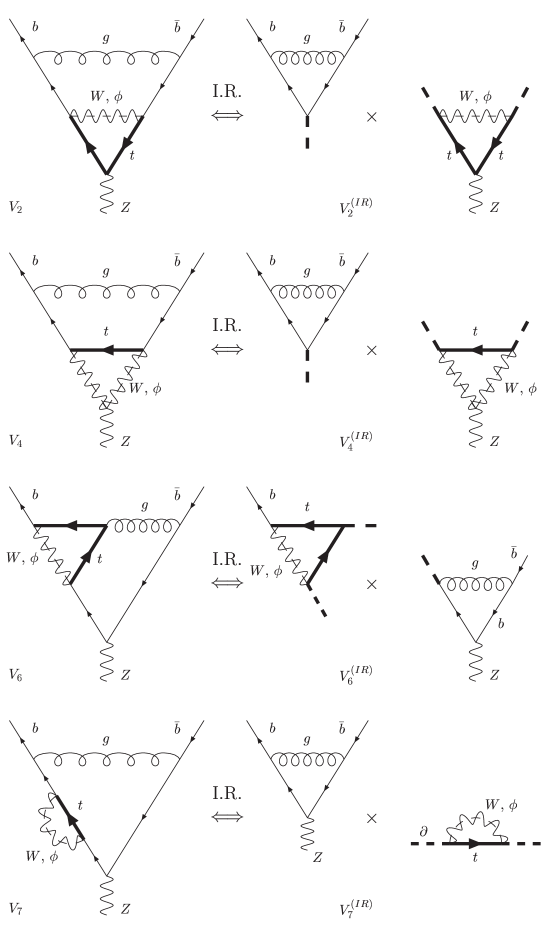
Figure 8: Extracting the infrared divergent pieces of the two-loop diagrams analytically. The infrared divergency of the two-loop diagram is the same as the infrared divergency of the product of the two one-loop diagrams obtained by “freezing” the common line in the loop momenta integration.

Once the IR separation is performed, the IR finite part ($V_{2}-V_{2}^{(IR)}$ etc.) can be calculated by numerical integration. For the numerical integration to be stable, one must make sure that the two components, e.g. $V_{2}$ and $V_{2}^{(IR)}$, have the same Feynman parameterization such that the singularities cancel already before the Feynman parameters integration. Then, the IR divergent part(e.g. $V_{2}^{(IR)}$) can easily be treated analytically, in general by using dimensional regularization to regularize the IR singularities.

For the case of the process considered in this example, a gluon mass regulator can also be used. This is possible because in this particular order in $\alpha_{s}$ the IR structure is the same as in the Abelian case, and a gluon mass regulator can be used without upsetting the Slavnov-Taylor identities.

It is still an open question if such an analytical separation of the infrared singularities can always be performed such that the numerical integration can be carried out, in the case of other processes with potentially more complicated IR structure. This question clearly requires further investigation.

4.3 Numerical results

We subtract the UV divergence of the diagrams of figure  7 by performing minimal subtractions of overall-divergences and sub-divergences. Further, we extract the IR divergences analytically, according to the discussion of the previous section. The tensor decomposition results in a set of convergent integrals over the remaining Feynman parameters, which can be carried out numerically.

Figure 9: Numerical results for the two-loop three-point function diagrams shown in figure 7. The UV divergences and sub-divergences are subtracted by minimal subtraction. The IR divergences are subtracted according to figure 8, so that the final result for diagrams $V_{2}$, $V_{4}$, $V_{6}$, and $V_{7}$ are the sum of the finite parts given in the plots plus the IR divergent one-loop contributions given in figure 8. There is an overall factor of $i\gamma_{\mu}(1-\gamma_{5})\alpha_{s}(g^{3}/12\cos\theta_{W})$. The solid line is the real part, and the dashed line is the imaginary part.

Because in the top mass range of physical interest the diagrams are not close to a threshold, the top mass dependency in the relevant range is relatively smooth, as it can be seen in figure 9. We give numerical values for these diagrams in table 1 for three values of the top mass — intermediary values can be well approximated by interpolation. In performing the numerical integration, we took $M_{W}=80.41$ GeV, $M_{Z}=91.187$ GeV, and the effective electroweak mixing angle $\sin^{2}\theta_{W}=.232$. For simplifying both the analytical and the numerical work, we neglected the $b$ mass, and in this limit all diagrams become proportional to $\gamma_{\mu}(1-\gamma_{5})$. It is perfectly possible to keep the exact $m_{b}$ dependency throughout the whole calculation at the price of dealing with longer expressions and more computing time; however the $b$ mass effect on the two-loop $Z\rightarrow b\bar{b}$ decay rate is expected to be very small.

The numerical results are given in table 1. As for the numerical accuracy and efficiency which can be attained, the results of table 1 are for a total of 26 individual Feynman diagrams ($W$ and $\phi$ exchange counted separately), each of them evaluated for 3 different values of the top mass. To carry out the numerical integration for this total of 78 two-loop individual Feynman graph evaluations with an accuracy of $10^{-3}$, a total of 100 hours computing time on a 600 MHz Pentium machine was used. Higher numerical accuracy can be obtained by simply using more computing power. The analytical tensor decomposition part, performed by a FORM computer algebra program (we also used a Schoonship version with similar results), takes about one hour.

diagram	$m_{t}=165$ GeV	$m_{t}=175$ GeV	$m_{t}=185$ GeV
$V_{1}$	$-1.009\cdot 10^{-3}$	$-7.187\cdot 10^{-4}$	$-4.057\cdot 10^{-4}$
$V_{2}-V_{2}^{(IR)}$	$(-2.873+i2.122)\cdot 10^{-3}$	$(-2.490+i1.147)\cdot 10^{-3}$	$(-2.087+i.09274)\cdot 10^{-3}$
$V_{3}$	$1.545\cdot 10^{-3}$	$2.255\cdot 10^{-3}$	$3.034\cdot 10^{-3}$
$V_{4}-V_{4}^{(IR)}$	$(1.215-i2.481)\cdot 10^{-2}$	$(1.242-i2.570)\cdot 10^{-2}$	$(1.266-i2.660)\cdot 10^{-2}$
$V_{5}$	$2.107\cdot 10^{-2}$	$2.469\cdot 10^{-2}$	$2.861\cdot 10^{-2}$
$V_{6}-V_{6}^{(IR)}$	$(3.089-i4.257)\cdot 10^{-2}$	$(3.500-i4.824)\cdot 10^{-2}$	$(3.950-i5.445)\cdot 10^{-2}$
$V_{7}-V_{7}^{(IR)}$	$(-.7778+i1.281)\cdot 10^{-2}$	$(-.8001+i1.349)\cdot 10^{-2}$	$(-.8232+i1.420)\cdot 10^{-2}$
$V_{8}$	$-1.059\cdot 10^{-3}$	$-1.474\cdot 10^{-3}$	$-1.942\cdot 10^{-3}$
$V_{9}$	$6.289\cdot 10^{-2}$	$6.703\cdot 10^{-2}$	$7.143\cdot 10^{-2}$
$V_{10}$	$-1.402\cdot 10^{-2}$	$-1.389\cdot 10^{-2}$	$-1.380\cdot 10^{-2}$

Table 1: Numerical values for the two-loop diagrams shown in figure 7. $V_{1}$–$V_{10}$ are the sums of the corresponding $W$ and $\phi$ exchange graphs. An overall color and coupling constant factor of $i\gamma_{\mu}(1-\gamma_{5})\alpha_{s}(g^{3}/12\cos\theta_{W})$ is understood. The UV and IR divergences are removed as discussed in the text. The numerical integration accuracy is $10^{-3}$. The evaluation of a total of 78 Feynman graph evaluations with this precision requires 100 hours computing time on a 600 MHz Pentium machine.

5 Conclusions

We described an algorithm for the tensor reduction of massive two-loop diagrams. It applies in principle to any massive two-loop graph, and it can be automatized in the form of a computer algebra program. The tensor decomposition algorithm results in a set of ten special functions $h_{i}$ which are defined in terms of one-dimensional integral representations. We described the numerical methods which are used for carrying out the remaining integrations.

By applying the analytical reduction and numerical integration to an important three-point example, $Z\rightarrow b\bar{b}$, we have shown that it can be used in realistic calculations, where several internal mass and external momenta scales are involved. This approach works for any such combination of kinematic variables, apart maybe from possible infrared complications.

In the context of the $Z\rightarrow b\bar{b}$ example given in this paper, we discussed the analytical separation of the infrared divergencies. Within our two-loop methods, if a process involves infrared singularities, these have to be dealt with in a special way because the numerical nature of our methods. It is an open question if this IR treatment can be generalized to other two-loop situations with potentially more complicated IR structure.

Aknowledgements

The work of A.G. was supported by the US Department of Energy. The work of Y.-P. Y. was supported partly by the US Department of Energy.

Appendix A

In section 2.2 we introduced two types of scalar functions which are involved in the tensor decomposition: ${\cal H}_{i}$ and $\tilde{\cal P}^{ab}_{\alpha_{1}\alpha_{2}\alpha_{3}}$. Then, we gave integral representations only for ${\cal H}_{i}$. The necessary $\tilde{\cal P}^{ab}_{2\,1\,1}$ scalar functions can be derived from the corresponding ${\cal H}_{i}$ by partial fractioning:

$$\tilde{{\cal P}}^{0\,0}_{2\,1\,1} = {\cal H}_{1}$$

$$\tilde{{\cal P}}^{1\,0}_{2\,1\,1} = {\cal H}_{2}$$

$$\tilde{{\cal P}}^{0\,1}_{2\,1\,1} = {\cal H}_{3}$$

$$\tilde{{\cal P}}^{2\,0}_{2\,1\,1} = {\cal H}_{4}+\frac{k^{2}}{n}\left[-(m_{1}^{2}+k^{2}){\cal H}_{1}-2{\cal H}_{2}+\tilde{\cal P}^{0\,0}_{1\,1\,1}\right]$$

$$\tilde{{\cal P}}^{1\,1}_{2\,1\,1} = {\cal H}_{5}+\frac{k^{2}}{2n}\left\{(m_{1}^{2}+m_{2}^{2}-m_{3}^{2}+k^{2}){\cal H}_{1}+2{\cal H}_{2}-\tilde{\cal P}^{0\,0}_{1\,1\,1}\right.$$

$$\left.\;\;\;\;\;\;\;\;\;\;\;\;\;\;\;\;\;\;\;\;\;\;\;\;\;\;\;\;\;\;\;\;\;\;\;\;\;\;\;\;\;\;\;\;\;\;\;\;\;\;\;\;\;\;\;\;\;\;\;\;+T_{2}(m_{1}^{2})\left[T_{1}(m_{2}^{2})-T_{1}(m_{3}^{2})\right]\right\}$$

$$\tilde{{\cal P}}^{0\,2}_{2\,1\,1} = {\cal H}_{6}+\frac{k^{2}}{n}\left[-m_{2}^{2}{\cal H}_{1}+T_{2}(m_{1}^{2})T_{1}(m_{3}^{2})\right]$$

$$\tilde{{\cal P}}^{3\,0}_{2\,1\,1} = {\cal H}_{7}+\frac{3k^{2}}{n+2}\left[-(m_{1}^{2}+k^{2}){\cal H}_{2}+\tilde{{\cal P}}^{1\,0}_{1\,1\,1}-2\tilde{{\cal P}}^{2\,0}_{2\,1\,1}\right]$$

$$\tilde{{\cal P}}^{2\,1}_{2\,1\,1} = {\cal H}_{8}+\frac{3k^{2}}{n+2}\left[-(m_{1}^{2}+k^{2}){\cal H}_{3}+{\cal P}^{0\,1}_{1\,1\,1}-2\tilde{{\cal P}}^{1\,1}_{2\,1\,1}\right]$$

$$\tilde{{\cal P}}^{1\,2}_{2\,1\,1} = {\cal H}_{9}+\frac{k^{2}}{n+2}\left[(m_{1}^{2}+m_{2}^{2}-m_{3}^{2}+k^{2}){\cal H}_{3}-m_{2}^{2}{\cal H}_{2}+2\tilde{{\cal P}}^{1\,1}_{2\,1\,1}-\tilde{\cal P}^{0\,1}_{1\,1\,1}\right.$$

$$\left.\;\;\;\;\;\;\;\;\;\;\;\;\;\;\;\;\;\;\;\;\;\;\;\;\;\;\;\;\;\;\;\;\;\;\;\;\;\;\;\;\;\;\;\;\;\;\;\;\;\;\;\;\;\;\;\;\;\;\;\;\;\;\;\;\;\;\;\;\;\;\;\;\;\;\;-2k^{2}T_{2}(m_{1}^{2})T_{1}(m_{3}^{2})\right]$$

$$\tilde{{\cal P}}^{0\,3}_{2\,1\,1} = {\cal H}_{10}+\frac{3k^{2}}{n+2}\left[-m_{2}^{2}{\cal H}_{3}+k^{2}T_{2}(m_{1}^{2})T_{1}(m_{3}^{2})\right]\;\;\;\;,$$ (18)

where $T_{1}$ and $T_{2}$ are the Euclidian one–loop tadpole integrals:

$$T_{1}(m^{2}) = \int d^{n}p\,\frac{1}{p^{2}+m^{2}}\;=\;-\pi^{2}\left(\pi m^{2}\right)^{\frac{\epsilon}{2}}\Gamma\left(-\frac{\epsilon}{2}\right)\,\frac{2m^{2}}{2+\epsilon}$$

$$T_{2}(m^{2}) = \int d^{n}p\,\frac{1}{(p^{2}+m^{2})^{2}}\;=\;\pi^{2}\left(\pi m^{2}\right)^{\frac{\epsilon}{2}}\Gamma\left(-\frac{\epsilon}{2}\right)\;\;.$$ (19)

In section 2.4, in order to simplify the discussion, we introduced the functions ${\cal P}^{ab}_{\alpha_{1}\alpha_{2}\alpha_{3}}$ which are related to $\tilde{\cal P}^{ab}_{\alpha_{1}\alpha_{2}\alpha_{3}}$ by a simple loop momentum shift:

$${\cal P}^{0\,0}_{2\,1\,1} = \tilde{{\cal P}}^{0\,0}_{2\,1\,1}$$

$${\cal P}^{1\,0}_{2\,1\,1} = -\tilde{{\cal P}}^{1\,0}_{2\,1\,1}-k^{2}\tilde{{\cal P}}^{0\,0}_{2\,1\,1}$$

$${\cal P}^{0\,1}_{2\,1\,1} = \tilde{{\cal P}}^{0\,1}_{2\,1\,1}$$

$${\cal P}^{2\,0}_{2\,1\,1} = \tilde{{\cal P}}^{2\,0}_{2\,1\,1}+2k^{2}\tilde{{\cal P}}^{1\,0}_{2\,1\,1}+(k^{2})^{2}\tilde{{\cal P}}^{0\,0}_{2\,1\,1}$$

$${\cal P}^{1\,1}_{2\,1\,1} = -\tilde{{\cal P}}^{1\,1}_{2\,1\,1}-k^{2}\tilde{{\cal P}}^{0\,1}_{2\,1\,1}$$

$${\cal P}^{0\,2}_{2\,1\,1} = \tilde{{\cal P}}^{0\,2}_{2\,1\,1}$$

$${\cal P}^{3\,0}_{2\,1\,1} = -\tilde{{\cal P}}^{3\,0}_{2\,1\,1}-3k^{2}\tilde{{\cal P}}^{2\,0}_{2\,1\,1}-3(k^{2})^{2}\tilde{{\cal P}}^{1\,0}_{2\,1\,1}-(k^{2})^{3}\tilde{{\cal P}}^{0\,0}_{2\,1\,1}$$

$${\cal P}^{2\,1}_{2\,1\,1} = \tilde{{\cal P}}^{2\,1}_{2\,1\,1}+2k^{2}\tilde{{\cal P}}^{1\,1}_{2\,1\,1}+(k^{2})^{2}\tilde{{\cal P}}^{0\,1}_{2\,1\,1}$$

$${\cal P}^{1\,2}_{2\,1\,1} = -\tilde{{\cal P}}^{1\,2}_{2\,1\,1}-k^{2}\tilde{{\cal P}}^{0\,2}_{2\,1\,1}$$

$${\cal P}^{0\,3}_{2\,1\,1} = \tilde{{\cal P}}^{0\,3}_{2\,1\,1}\;\;.$$ (20)

The functions with $\alpha_{1}=\alpha_{2}=\alpha_{3}=1$ which appear in the relations 18 can be calculated by partial $p$ (eq. 15). For simplifying the notation, we omitted in the above formulae the mass and momentum arguments of the functions ${\cal H}_{i}(m_{1},m_{2},m_{3};k^{2})$, ${\cal P}^{a\,b}_{\alpha_{1}\,\alpha_{2}\,\alpha_{3}}(m_{1},m_{2},m_{3};k^{2})$, and $\tilde{{\cal P}}^{a\,b}_{\alpha_{1}\,\alpha_{2}\,\alpha_{3}}(m_{1},m_{2},m_{3};k^{2})$, and understand that these arguments appear in this same order in all relations.

Appendix B

The integral representations of the ten special functions functions $h_{i}$, given in eqs. 8, are built from the following functions:

$$\tilde{g}(m_{1},m_{2},m_{3};k^{2};x) = Sp(\frac{1}{1-y_{1}})+Sp(\frac{1}{1-y_{2}})+y_{1}\log{\frac{y_{1}}{y_{1}-1}}+y_{2}\log{\frac{y_{2}}{y_{2}-1}}$$

$$\tilde{f_{1}}(m_{1},m_{2},m_{3};k^{2};x) = \frac{1}{2}\left[-\frac{1-\mu^{2}}{\kappa^{2}}+y_{1}^{2}\log{\frac{y_{1}}{y_{1}-1}}+y_{2}^{2}\log{\frac{y_{2}}{y_{2}-1}}\right]$$

$$\tilde{f_{2}}(m_{1},m_{2},m_{3};k^{2};x) = \frac{1}{3}\left[-\frac{2}{\kappa^{2}}-\frac{1-\mu^{2}}{2\kappa^{2}}-\left(\frac{1-\mu^{2}}{\kappa^{2}}\right)^{2}\right.$$

$$\;\;\;\;\;\;\;\;\;\;\;\;\;\;\;\;\;\;\;\;\;\;\;\;\;\;\;\;\;\;\;\;\;\;\;\;\left.+y_{1}^{3}\log{\frac{y_{1}}{y_{1}-1}}+y_{2}^{3}\log{\frac{y_{2}}{y_{2}-1}}\right]$$

$$\tilde{f_{3}}(m_{1},m_{2},m_{3};k^{2};x) = \frac{1}{4}\left[-\frac{4}{\kappa^{2}}-\left(\frac{1}{3}+\frac{3}{\kappa^{2}}\right)\left(\frac{1-\mu^{2}}{\kappa^{2}}\right)-\frac{1}{2}\left(\frac{1-\mu^{2}}{\kappa^{2}}\right)^{2}-\left(\frac{1-\mu^{2}}{\kappa^{2}}\right)^{3}\right.$$ (21)

$$\left.\;\;\;\;\;\;\;\;\;\;\;\;\;\;\;\;\;\;\;\;\;\;\;\;\;\;\;\;\;\;\;\;\;\;\;\;+y_{1}^{4}\log{\frac{y_{1}}{y_{1}-1}}+y_{2}^{4}\log{\frac{y_{2}}{y_{2}-1}}\right]\;\;,$$

where we use the following notations:

$$y_{1,2} = \frac{1+\kappa^{2}-\mu^{2}\pm\sqrt{\Delta}}{2\kappa^{2}}$$

$$\Delta = (1+\kappa^{2}-\mu^{2})^{2}+4\kappa^{2}\mu^{2}-4i\kappa^{2}\eta\;\;,$$ (22)

and

$$\mu^{2} = \frac{ax+b(1-x)}{x(1-x)}$$

$$a = \frac{m_{2}^{2}}{m_{1}^{2}}\,,\;\;\;\;b\;=\;\frac{m_{3}^{2}}{m_{1}^{2}}\,,\;\;\;\;\kappa^{2}\;=\;\frac{k^{2}}{m_{1}^{2}}\;\;.$$ (23)

In the above expressions, one special case must be treated separately, namely $k^{2}=0$. The $h_{i}$ functions have a smooth limit for $k^{2}\rightarrow 0$. For the purpose of numerical evaluation, it is useful to use a Taylor expansion of the functions $\tilde{g}$, $\tilde{f}_{1}$, $\tilde{f}_{2}$, and $\tilde{f}_{3}$ around $k^{2}=0$ for extremely small values of $k^{2}$, where a direct evaluation by means of the exact expressions given above would be affected by large cancellations. It can be checked that this limit is regular and our approach reduces to the functions introduced by van der Bij and Veltman in ref. [10].

References

- [1] Z. Bern, L. Dixon, D.A. Kosower, JHEP 0001 (2000) 027; J.B. Tausk, Phys. Lett. B469 (1999) 225; C. Anastasiou, T. Gehrmann, C. Oleari, E. Remiddi, J.B. Tausk, hep-ph/0003261; V.A. Smirnov, O.L. Veretin Nucl. Phys. B566 (2000) 469; J.A.M. Vermaseren, S.A. Larin, T. van Ritbergen, Phys. Lett. B405 (1997) 327; Phys. Lett. B404 (1997) 153; Phys. Lett. B400 (1997) 379.
- [2] G. Weiglein, R. Scharf, M. Bohm, Nucl. Phys. B416 (1994) 606.
- [3] S. Bauberger and G. Weiglein, Phys. Lett. B419 (1998) 333; Nucl. Instrum. Meth. A389 (1997) 318.
- [4] A. Ghinculov and Y.-P. Yao, Nucl. Phys. B516 (1998) 385.
- [5] A. Ghinculov and J.J. van der Bij, Nucl. Phys. B436 (1995) 30; A. Ghinculov, Phys. Lett. B337 (1994) 137; (E) B346 (1995) 426; Nucl. Phys. B455 (1995) 21.
- [6] F.A. Berends, M. Buza, M. Böhm and R. Scharf, Z. Phys. C63 (1994) 227.
- [7] R. Harlander, T. Seidensticker, M. Steinhauser, Phys. Lett. B426 (1998) 125; J. Fleischer, O.V. Tarasov, F. Jegerlehner, P. Raczka, Phys. Lett. B293 (1992) 437; J. Fleischer, F. Jegerlehner, M. Tentyukov, O. Veretin, Phys. Lett. B459 (1999) 625.
- [8] A. Ghinculov and Y.-P. Yao, hep-ph/9910422.
- [9] A. Ghinculov and Y.-P. Yao, hep-ph/0002211; hep-ph/0004201.
- [10] J.J. van der Bij and M. Veltman, Nucl. Phys. B231 (1984) 205.