Abstract

We report on QCD radiative corrections to the process $p\bar{p}\rightarrow Zb\bar{b}$ in the approximation in which the $b$ quark is considered massless. The implementation of this process in the general purpose Monte Carlo program MCFM is discussed in some detail. These results are used to investigate backgrounds to Higgs boson production in the $ZH$ channel. We investigate the Higgs mass range ($100{\;\rm GeV}<m_{H}<130{\;\rm GeV}$) for the Tevatron running at $\sqrt{s}=2{\;\rm TeV}$.

1 Introduction

In this paper we report on the calculation of the strong radiative corrections to the process

$$p+\bar{p}\rightarrow Z+b+\bar{b}\ .$$ (1)

These results are obtained from a Monte Carlo program which allows us to obtain predictions for any infra-red safe variable. Since the decays of the $Z$ are included we can perform cuts on the transverse momenta and rapidities of the final state leptons as well as on the properties of the jets present in the event. This discussion is similar to the calculation

$$p+\bar{p}\rightarrow W+b+\bar{b}\ ,$$ (2)

presented in ref. [1], although there are some differences. Ref. [1] can be seen as a first step towards the calculation of a vector boson plus 2 jets at ${\cal O}(\alpha_{s}^{3})$, where the underlying partonic process contains only quarks in the initial state. When considering the production of $Zb{\bar{b}}$ we must also consider initial states containing two gluons, a further stepping-stone towards a general $V+$ 2 jet program. With this in mind, we shall present our method in some detail, with a general outline in Section 2 and further details presented in the Appendix.

Much effort has been devoted to the study of Higgs production at the Tevatron running at $\sqrt{s}=2$ TeV [2]. These studies indicate that, given enough luminosity, a light Higgs boson can be discovered at the Tevatron using the associated production channels $WH$ and $ZH$. In Section 3 we perform an analysis in the $ZH$ channel that incorporates as many of the backgrounds as possible at next-to-leading order. Whilst we use no detector simulation and do not attempt to include backgrounds due to particle misidentification, the results presented here can provide a normalization for more experimentally realistic studies. This is of importance since more detailed studies are often performed using shower Monte Carlo programs which can give misleading results for well separated jets.

2 Calculational overview

In this section we will outline the implementation of the matrix elements in our Monte Carlo program. We separate the discussion according to the three types of contribution: the lowest order (Born) processes, the virtual (loop) corrections and the real corrections associated with additional soft or collinear radiation.

2.1 Born processes

The Born processes which we are considering are

$$q+\bar{q}\rightarrow Z+b+\bar{b}$$

$$g+g\rightarrow Z+b+\bar{b}$$ (3)

which are illustrated in Fig. 1.

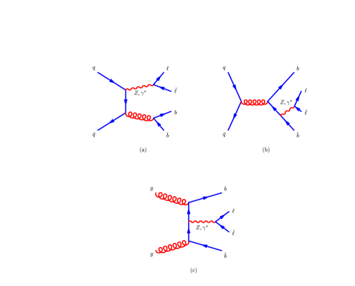
Figure 1: Representative diagrams contributing to $Zb{\bar{b}}$ production at lowest order. A complete gauge-invariant set of diagrams is included in the actual calculation.

For the $q\bar{q}$ case, the set of diagrams represented in (a) is the same as that previously implemented for $Wb\bar{b}$ production in ref. [1]. The diagrams in (b) are related to those in (a) by crossing. Diagrams (b) are absent in the $Wb{\bar{b}}$ case since a $W$ does not directly couple to a $b{\bar{b}}$ pair. For the same reason, the $gg$ process (c) is also not present in the case of $Wb\bar{b}$ production and these diagrams introduce a new set of matrix elements. In all of the matrix elements we will use the massless approximation for the $b$-quarks. We expect this to be a good description for $b{\bar{b}}$ pairs produced with a large invariant mass, $m_{b{\bar{b}}}$. This expectation is borne out by Fig. 2 where lowest order predictions with and without the $b$-quark mass are compared. As expected the corrections are of order $4m_{b}^{2}/m_{b\bar{b}}^{2}$. Note that Fig. 2 may overestimate the mass effect since a fixed mass, rather than a running mass which is smaller at high scale, is used. The basic jet cuts used in Fig. 2 to define the $b\bar{b}$ jets are,

$$|y_{\mbox{jet}}| < 2.5\ ,$$

$$|p^{T}_{\mbox{jet}}| > 15{\;\rm GeV}\ ,$$

$$\Delta R > 0.7$$ (4)

where as usual

$$\Delta R=\sqrt{[\Delta\eta^{2}+\Delta\phi^{2}]}\;.$$ (5)

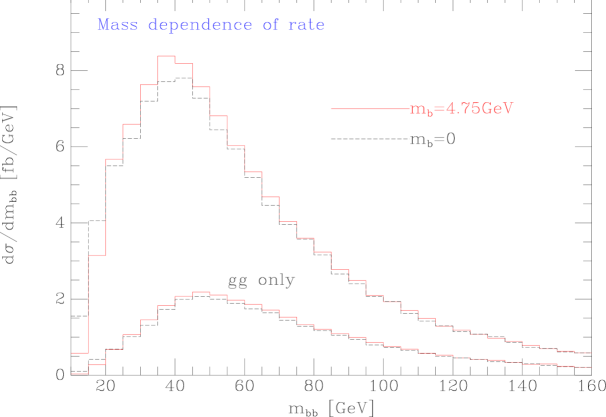
Figure 2: Lowest order predictions showing the validity of the zero mass approximation

Fig. 2 also illlustrates the relative importance of the two sub-processes in Eq. (2.1). The total cross-section and the contribution from $gg$-initiated processes are shown separately, binned according to the $b{\bar{b}}$ invariant mass. If we examine the total cross-sections (integrated over a large range, $10{\;\rm GeV}<m_{b{\bar{b}}}<160{\;\rm GeV}$), we find that the gluon-gluon contribution is $36\%$ of the quark-antiquark result. However, when we are later interested in examining this process as a background to a $ZH(\to b{\bar{b}})$ signal, we will be interested in the cross-sections over a limited range of $m_{b{\bar{b}}}$ close to a Higgs mass $m_{H}$, where $100{\;\rm GeV}<m_{H}<130{\;\rm GeV}$. We can see from the figure that in this region the $gg$ contribution is a much more significant fraction of the total, roughly $60\%$ of the $q{\bar{q}}$ cross-section in a window around $m_{H}=110{\;\rm GeV}$. The reason for the importance of the $gg$ process in this region can be understood from the contributing diagrams. By examination of Fig. 1(c) we see that, in contrast to the other diagrams in Fig. 1, $m_{b{\bar{b}}}$ may be large whilst keeping all propagators on-shell.

2.2 Real corrections

The real matrix elements of Nagy and Trocsanyi (NT) given in ref. [3] are implemented using a subtraction procedure [4] which follows closely the treatment of Ref. [5]. To illustrate our method, we outline the subtraction terms that are needed for one particular piece, namely the leading colour contribution to the $gg$ process. The actual numerical calculation that we have implemented includes the full matrix elements, not just this leading colour piece.

We shall label the momenta of the partons as follows,

$$g(-p_{1})+g(-p_{2})\to Z(p_{34})+b(p_{5})+{\bar{b}}(p_{6})+g(p_{7}),$$ (6)

where all momenta are considered outgoing. In leading colour, it is sufficient to consider one ordering of the gluons along the fermion line, and to obtain the remaining terms by permutation of the gluons [6]. The real matrix elements are given by,

$$|{\cal M}_{\rm real}|^{2} = 8e^{4}g^{6}C_{F}N^{3}\times\left(\sum_{\rm(6~{}perms)}\left|A(5_{q}^{h_{5}},1_{g}^{h_{1}},2_{g}^{h_{2}},7_{g}^{h_{7}},6_{\bar{q}}^{h_{6}})\right|^{2}+{\cal O}\left(\frac{1}{N^{2}}\right)\right)$$ (7)

$$\equiv \sum_{\rm(6~{}perms)}|{\cal M}_{5}(1_{g},2_{g},7_{g})|^{2}+{\cal O}\left(C_{F}N\right),$$

where we have used the (NT) notation for the tree-level amplitude $A$ (see Eqs. (NT:A43-A49)) and for simplicity we have suppressed all couplings of the $Z$ boson and the sum over quark and lepton helicities. As usual $C_{F}=4/3$ and $N=3$ is the number of colours. The neglected terms are subleading in $N$. Eq. (7) is very similar to the leading-order term,

$$|{\cal M}_{\rm LO}|^{2} = 8e^{4}g^{4}C_{F}N^{2}\times\left(\sum_{\rm(2~{}perms)}\left|m(5_{q}^{h_{5}},1_{g}^{h_{1}},2_{g}^{h_{2}},6_{\bar{q}}^{h_{6}})\right|^{2}+{\cal O}\left(\frac{1}{N^{2}}\right)\right)$$ (8)

$$\equiv \sum_{\rm(2~{}perms)}|{\cal M}_{4}(1_{g},2_{g})|^{2}+{\cal O}\left(C_{F}\right),$$

which we will use to construct the subtraction terms.

2.2.1 Dipole enumeration

The matrix elements in Eq. (7) become singular when gluon 7 becomes soft and/or collinear with the quarks or either of the other gluons. There are a number of methods for cancelling these singularities at next-to-leading order [7] and we choose to use the dipole subtraction method of Catani and Seymour [5]. In this approach, the dipoles provide a convenient and efficient way of enumerating the singularities and cancelling them in a local fashion, including spin correlations.

A dipole consists of 3 partons, the first two of which combine to form the emitter parton, $\widetilde{ai}$, and the third is the spectator $b$. The construction of the dipoles starts [4] from the eikonal factors present in the soft limit which are rewritten as,

$$\frac{2p_{a}p_{b}}{p_{a}p_{i}\;p_{b}p_{i}}\equiv\frac{2p_{a}p_{b}}{p_{a}p_{i}+p_{b}p_{i}}\Big{[}\frac{1}{p_{a}p_{i}}+(a\leftrightarrow b)\Big{]}.$$ (9)

The first term on the right hand side corresponds to the soft limit of the dipole with emitter $\widetilde{ai}$ and spectator $b$. The full dipole is given by the extension of Eq. (9) to include collinear emission. The dipole must be labelled by the parton type of both emitter and emitted parton, as well as whether the partons lie in the initial or final state. For instance, the notation ${\cal D}_{ii,\,gg}^{17,2}$ refers to a dipole where $\widetilde{17}$ is the initial-state gluonic emitter splitting into gluon $1$ and parton $7$, with respect to spectator parton $2$.

The dipole structure of the subtraction terms can be understood from the soft gluon limit of the matrix elements (7). In the soft limit of a single colour ordering (permutation), gluon 7 can have singularities with neighbouring partons only. Each of the six permutations therefore gives rise to two dipoles, leading to twelve terms in all. Hence we find,

$$|{\cal M}|^{2}_{\rm dipole}=N\left[{\cal D}_{ii,\,gg}^{17,2}+{\cal D}_{ii,\,gg}^{27,1}+{\cal D}_{if,\,gg}^{17,5}+{\cal D}_{fi,\,qq}^{57,1}+{\cal D}_{if,\,gg}^{27,6}+{\cal D}_{fi,\,qq}^{67,2}\right]\times\left|{\cal M}_{4}(1_{g},2_{g})\right|^{2}+(1\leftrightarrow 2)$$ (10)

where the dipole functions are listed explicitly in Appendix A.

2.3 Virtual corrections

The virtual corrections to the processes in Eq. (2.1) are taken from the work of BDK, (Bern, Dixon and Kosower [8]). For other work on these parton subprocesses, see also ref. [9]. In this paper the ultraviolet, infra-red and collinear singularities are controlled by continuing the dimension of space-time to $d=4-2\epsilon$ using the four-dimensional helicity scheme. The structure of the Monte Carlo program is such that virtual terms are combined with the integrals of the dipole subtraction pieces defined above. When added together, $\epsilon$-poles cancel and a finite result is obtained.

To demonstrate this explicitly, we will examine the leading colour contribution to the 1-loop diagrams. From BDK the leading $N$-contribution from the loop diagrams is (cf. BDK, Eq. (2.12)),

$${\rm Re}\left(2{\cal M}_{\rm LO}{\cal M}^{*}_{\rm 1-loop}\right)=8e^{4}g^{4}C_{F}N^{3}\left(\frac{\alpha_{S}}{2\pi}\right)(4\pi)^{2}$$

$$\times\Biggl{[}A_{6}^{\rm tree\,*}(5_{q},1_{g},2_{g},6_{\bar{q}})A_{6;1}(5_{q},1_{g},2_{g},6_{\bar{q}})+{\cal O}\left(\frac{1}{N}\right)\Biggr{]}+(1\leftrightarrow 2).$$ (11)

Extracting only the pole pieces from the leading term (see BDK, Eqs. (8.5) and (8.7), together with the renormalization in Eq. (6.5)) yields,

$${\rm Re}\left(2{\cal M}_{\rm LO}{\cal M}_{\rm 1-loop}^{*}\right)^{\rm pole}=-\left(\frac{\alpha_{S}N}{2\pi}\right)|{\cal M}(1_{g},2_{g})|^{2}\times\Biggl{[}$$ (12)

$$\frac{1}{\epsilon^{2}}\left(\left(\frac{s_{15}}{\mu^{2}}\right)^{-\epsilon}+\left(\frac{s_{12}}{\mu^{2}}\right)^{-\epsilon}+\left(\frac{s_{26}}{\mu^{2}}\right)^{-\epsilon}\right)+\frac{3}{2\epsilon}\left(\frac{s_{34}}{\mu^{2}}\right)^{-\epsilon}+\frac{1}{3\epsilon}\left(11-\frac{2n_{f}}{N}\right)+\frac{7}{2}\Biggr{]}+(1\leftrightarrow 2),$$

where we have adopted the usual definition $s_{ij}=2p_{i}\cdot p_{j}$. We are now in a position to make a comparison with the dipole terms that we presented in the previous section, Eq. (10). Inserting the appropriate integrals (the functions ${\cal V}^{end}$ from Appendix A) we find the counterterm from the real contribution to be,

$$|{\cal M}|^{2}_{\rm counter} = \left(\frac{\alpha_{S}N}{2\pi}\right)|{\cal M}(1_{g},2_{g})|^{2}\times\frac{1}{2}\times\Biggl{[}$$

$$\frac{2}{\epsilon^{2}}\left(\frac{s_{12}}{\mu^{2}}\right)^{-\epsilon}+\frac{1}{3\epsilon}\left(11-\frac{2n_{f}}{N}\right)-\frac{\pi^{2}}{3}$$

$$+ \frac{2}{\epsilon^{2}}\left(\frac{s_{15}}{\mu^{2}}\right)^{-\epsilon}+\frac{3}{2\epsilon}\left(\frac{s_{15}}{\mu^{2}}\right)^{-\epsilon}+\frac{1}{6\epsilon}\left(11-\frac{2n_{f}}{N}\right)-\frac{\pi^{2}}{3}+3$$

$$+ \frac{2}{\epsilon^{2}}\left(\frac{s_{26}}{\mu^{2}}\right)^{-\epsilon}+\frac{3}{2\epsilon}\left(\frac{s_{26}}{\mu^{2}}\right)^{-\epsilon}+\frac{1}{6\epsilon}\left(11-\frac{2n_{f}}{N}\right)-\frac{\pi^{2}}{3}+3\Biggr{]}+(1\leftrightarrow 2),$$

When we add these two contributions together, we see that the $\epsilon$-poles cancel, leaving a finite term that is a combination of logarithms and constants multiplying the lowest order squared matrix elements,

$${\rm Re}\left(2{\cal M}_{\rm LO}{\cal M}^{*}_{\rm 1-loop}\right)^{\rm pole}+|{\cal M}|^{2}_{\rm counter}=$$ (13)

$$\left(\frac{\alpha_{S}N}{2\pi}\right)|{\cal M}(1_{g},2_{g})|^{2}\times\Biggl{[}\frac{3}{4}\ln\left(\frac{s_{34}}{s_{15}}\right)+\frac{3}{4}\ln\left(\frac{s_{34}}{s_{26}}\right)-\frac{\pi^{2}}{2}-\frac{1}{2}\Biggr{]}+(1\leftrightarrow 2).$$

This result exemplifies the cancellation that occurs throughout our calculation, both at sub-leading colour and in the other $q{\bar{q}}$ initiated sub-process (the details of which we have omitted here for brevity). In general, when the poles present in [8] are added to the integrated dipoles given in Appendix A, the result is extra finite terms proportional to the lowest order matrix elements.

3 Results

3.1 Basic features

The standard model is specified by three gauge couplings; the top quark mass also leads to large corrections to tree graph results. For our purposes we will replace these four parameters by $M_{W},M_{Z},\alpha(M_{Z})$ and $G_{F}$, the values of which are given in Table 1.

$M_{Z},\Gamma_{Z}$	$91.187,2.49{\;\rm GeV}$	$\alpha(M_{Z})$	1/128.89
$M_{W},\Gamma_{W}$	$80.41,2.06{\;\rm GeV}$	$G_{F}$	$1.16639\times 10^{-5}$

Table 1: Basic input parameters.

The coupling constants $e,g_{W}$ and $\sin^{2}\theta_{W}$ are derived from these input parameters according to the definitions below,

$$e^{2} = 4\pi\alpha(M_{Z})$$

$$g^{2}_{W} = 4\sqrt{2}G_{F}M_{W}^{2}$$

$$\sin^{2}\theta_{W} = \frac{e^{2}}{g^{2}_{W}}\;.$$ (14)

When defined in this way, these are effective parameters which include the leading effects of top quark loops [10]. In addition, we use the MRS98 parton distribution set [11] with $\alpha_{S}(M_{Z})=0.1175$.

We apply our results to the phenomenological study of the $Zb{\bar{b}}$ background to $ZH$ production. We consider the channel $Z\rightarrow\nu\bar{\nu}$ which has a branching ratio of about $\sim 20\%$; the signature in this mode is a $b\bar{b}$-pair and missing transverse energy, which we denote by $\mathop{\not\!\!E_{T}}$. For convenience we impose the following cuts on our Monte Carlo simulation, and these will apply to all the results given in this section. We first require the observation of a $b$ and a $\bar{b}$ jet well separated from each other and from the direction in the transverse plane of the missing energy. The cuts we impose (in addition to the basic jet cuts of Eq. (2.1)) are,

$$\begin{array}[]{rcl}|y_{b}|,|y_{\bar{b}}|&<&2\ ,\\ |p^{T}_{b}|,|p^{T}_{\bar{b}}|&>&15{\;\rm GeV}\ ,\\ \phi_{\;\mathop{\not\!\!E_{T}},b},\phi_{\;\mathop{\not\!\!E_{T}},\bar{b}},&>&0.5,\\ \Delta R&>&0.7,\\ |\mathop{\not\!\!E_{T}}|&>&35{\;\rm GeV}.\\ \end{array}$$ (15)

where $\phi_{\;\mathop{\not\!\!E_{T}},b}$ is the azimuthal angle between the $b$-jet direction and the direction of the missing $E_{T}$. We also reject events which have additional jets in the observed region

$$|y_{\mbox{jet}}| < 2.5\ ,$$

$$|p^{T}_{\mbox{jet}}| > 15{\;\rm GeV}.$$ (16)

We first examine the distribution of the cross-section as a function of the $b\bar{b}$ mass. Our results are presented at leading and next-to-leading order for a renormalization and factorization scale $\mu=100$ GeV and also for a much smaller choice $\mu=20$ GeV in Figs. 3 and 4.

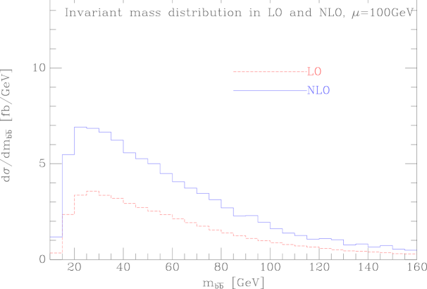
Figure 3: The $b\bar{b}$ mass distribution in $b\bar{b}$ + missing energy events with the renormalization and factorization scale $\mu=100{\;\rm GeV}$.

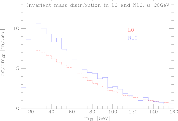
Figure 4: The $b\bar{b}$ mass distribution in $b\bar{b}$ + missing energy events with the renormalization and factorization scale $\mu=20{\;\rm GeV}$.

This smaller scale is chosen because, as can be seen in Fig. 4, for this scale choice the distributions at LO and NLO are comparable for $100<m_{b{\bar{b}}}<160$ GeV. We see that there is both a significant enhancement in the total cross-section and a change in the shape of the distribution when including the radiative corrections. Moreover, for the lower choice of scale, the total cross-section in the range $20<m_{b{\bar{b}}}<160$ GeV is even larger and there is a steepening of the distribution towards the peak at low $m_{b\bar{b}}$.

To further investigate the issue of scale dependence in this process, we consider an integral of the cross-section over a restricted range of $m_{b\bar{b}}$. We will consider such integrals in our analysis of the Higgs search, where we shall integrate around the mass of the putative Higgs boson. In particular, we will integrate over

$$m_{H}-\sqrt{2}\Delta<m_{b\bar{b}}<m_{H}+\sqrt{2}\Delta$$ (17)

where $\Delta$ is the mass resolution of the $b\bar{b}$-pair. We assume that $\Delta=0.1\times m_{H}$ and perform a gaussian smearing with this resolution. The scale dependence of the cross-section is shown in Fig. 5.

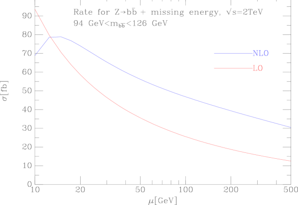
Figure 5: The scale dependence of the $Zb{\bar{b}}$ result at both leading and next-to-leading order, with $94<m_{b{\bar{b}}}<126$ GeV, appropriate for $M_{H}=110$ GeV with $\Delta=11$ GeV.

For low values of the renormalization and factorization scale $\mu$ the NLO cross-section peaks; it is equal to the lowest order result at $\mu\approx 15$ GeV.

To conclude our discussion of the general features of the $Zb{\bar{b}}$ calculation at NLO, we assess the relative importance of the different sub-processes. We have already seen that at leading order the $gg$ process provides a significant contribution to the cross-section, particularly for higher values of $m_{b{\bar{b}}}$. For this reason, in Fig. 6 we show the cross-section binned by $m_{b{\bar{b}}}$ and separated into the contribution of the $gg$ component of parton luminosity and the contribution of the rest (beyond leading order we also have $qg$ initial states).

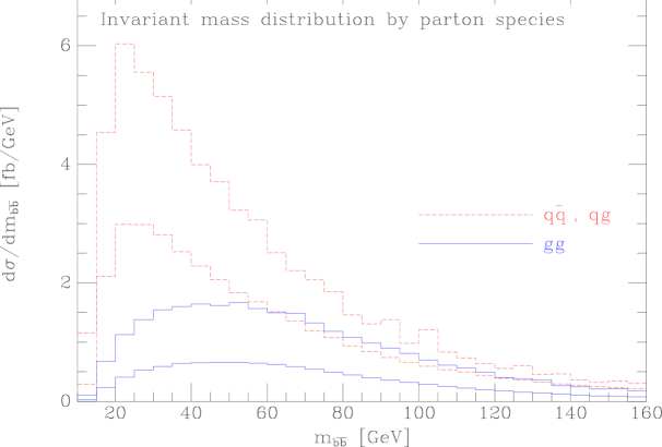
Figure 6: The contribution of the different parton-parton sub-processes to the cross-section, with the renormalization and factorization scale $\mu=100$ GeV. The lower curves represent the leading order results.

This figure shows that for the interesting range, $m_{b\bar{b}}\sim 100$ GeV, the $gg$ contribution is even more important, relative to the other sub-processes, than at leading order. In fact, if we divide the next-to-leading order curve by the leading order one to obtain the ‘$K$-factor’ we find that for $m_{b\bar{b}}>60$ GeV the ratio $K_{q{\bar{q}}/qg}\approx 1.7$ whilst $K_{gg}\approx 2.5$.

3.2 Higgs search

Previous studies [2, 12, 13] have shown that the channel $ZH$ where the $Z$ decays in neutrinos (observed in the detector as missing transverse energy) and the Higgs boson decays to $b\bar{b}$ can give a significant signal for the standard model Higgs boson with a mass below $130{\;\rm GeV}$.

The largest background to this signal is the $Zb{\bar{b}}$ process that we have discussed above. After this QCD background, the largest other background at $2{\;\rm TeV}$ is from the diboson process $Z^{0}(\rightarrow\nu\bar{\nu})Z(\rightarrow b\bar{b})$. Significantly smaller backgrounds come from the processes $W^{\pm*}(\to t(\rightarrow bW^{+})\bar{b})$ and $q^{\prime}t(\rightarrow bW^{+}){\bar{b}}$, where in each case the $W$ boson decays leptonically, but the charged lepton is not observed. In addition contributions to the signal are present from $p\bar{p}\rightarrow WH$ where the $W$-decay lepton is missed; correspondingly there are contributions to the background from $p\bar{p}\rightarrow Wb\bar{b}$ and $p\bar{p}\rightarrow WZ$.

In our analysis, we will calculate the significances using our parton level Monte Carlo MCFM in which the signal and largest backgrounds are calculated beyond the leading order. In order to calculate the signal we require the Higgs branching ratio into $b\bar{b}$ pairs, which is a strong function of the Higgs mass. The values of the branching ratio for the four values of the Higgs mass that we will study, as well as additional parameters used to calculate the other backgrounds, are shown in Table 2.

$m_{t},\Gamma_{t}$	$175,1.4{\;\rm GeV}$	$\sin^{2}\theta_{W}$	0.22853
$V_{ud}$	0.97500	Higgs mass (br)	$100{\;\rm GeV},(0.8119)$
$V_{us}$	0.22220	Higgs mass (br)	$110{\;\rm GeV},(0.7697)$
$V_{cd}$	0.22220	Higgs mass (br)	$120{\;\rm GeV},(0.6778)$
$V_{cs}$	0.97500	Higgs mass (br)	$130{\;\rm GeV},(0.5254)$

Table 2: Additional parameters used for the signal and background calculations for the Higgs search.

In order that our normalizations are clear, in Table 3 we show the total cross-section for each process, together with the results when appropriate branching ratios and lepton flavour sums are included. The values shown for the $Wb\bar{b}$ and $Zb\bar{b}$ processes only have the basic cuts, Eq. (2.1); for $t\bar{t},WH$ and $ZH$ the rates shown are the total cross sections with no cuts.

Process	$\sigma$ [fb]	With BR	$\sigma_{BR}$ [fb]
$WH$, $m_{H}=100$	$274$	$W^{+}(\to e^{+}\nu)H(\to b{\bar{b}})\times 4$	48.9
$ZH$, $m_{H}=100$	$162$	$Z(\to\nu_{e}{\bar{\nu}}_{e})H(\to b{\bar{b}})\times 3$	25.3
$Zb\bar{b}$, $60<m_{b\bar{b}}<160$	5290	$Z(\to\nu_{e}{\bar{\nu}}_{e})b\bar{b}\times 3$	1010
$ZZ$	1240	$Z(\to\nu_{e}{\bar{\nu}}_{e})Z(\to b{\bar{b}})\times 3\times 2$	71.4
$Wb\bar{b}$, $60<m_{b\bar{b}}<160$	8060	$W^{+}(\to e^{+}\nu)b\bar{b}\times 4$	1770
$WZ$	3600	$W^{+}(\to e^{+}\nu)Z(\to b{\bar{b}})\times 4$	119
$W^{\pm*}(\to t(\rightarrow bW^{+})\bar{b})$	449	$W^{\pm*}(\to t(\to bW^{+}(\to e^{+}\nu)){\bar{b}})\times 4$	98.8
$q^{\prime}t(\rightarrow bW^{+}){\bar{b}}$	81	$q^{\prime}t(\to bW^{+}(\to e^{+}\nu)){\bar{b}}\times 4$	35.6

Table 3: Values of the total cross-sections for normalization purposes

For each choice of the Higgs boson mass, the signal and backgrounds are integrated over an $m_{b\bar{b}}$ masss range as in Eq. (17). For the backgrounds we also reject events with additional observed leptons,

$$|y_{l}| < 2,$$

$$|p^{T}_{l}| > 10{\;\rm GeV}.$$ (18)

Our results at $2{\;\rm TeV}$ are given in Table 4, where we have used a double $b$-tagging efficiency $\epsilon_{b\bar{b}}=0.45$.

$m_{H}$ [GeV]	100	110	120	130
$Z^{0}(\rightarrow\nu\bar{\nu})H(\rightarrow b\bar{b})$	$5.8$	$4.4$	$2.9$	$1.8$
$W(\rightarrow\ell\nu)H(\rightarrow b\bar{b})$	$0.7$	$0.5$	$0.3$	$0.2$
Total $S$	$6.5$	$4.9$	$3.2$	$2.0$
$Z^{0}(\rightarrow\nu\bar{\nu})g^{*}(\rightarrow b\bar{b})$	$23.3$	$21.0$	$17.5$	$15.8$
$Z^{0}(\rightarrow\nu\bar{\nu})Z(\rightarrow b\bar{b})$	$10.8$	$6.9$	$3.3$	$1.4$
$W^{\pm}(\rightarrow\ell\bar{\nu})g^{*}(\rightarrow b\bar{b})$	$2.7$	$2.4$	$1.6$	$1.1$
$W^{\pm}(\rightarrow\ell\bar{\nu})Z(\rightarrow b\bar{b})$	$1.4$	$0.8$	$0.4$	$0.2$
$W^{\pm*}(\to t(\rightarrow bW^{+})\bar{b})$	$0.6$	$0.6$	$0.6$	$0.6$
$q^{\prime}t(\rightarrow bW^{+}){\bar{b}}$	$0.2$	$0.2$	$0.2$	$0.2$
Total $B$	$39.0$	$31.9$	$23.6$	$19.3$
$S/B$	$0.17$	$0.15$	$0.14$	$0.11$
$S/\sqrt{B}$	$1.04$	$0.87$	$0.66$	$0.46$

Table 4: Signal, backgrounds and significance for the $Z$-channel at $\sqrt{s}=2~{}{\;\rm TeV}$

When we compare these results to those of the SUSY-Higgs study [2] we immediately see a difference in some of the channels. In particular, by including the radiative corrections to the $Zb{\bar{b}}$ process we have increased this background considerably. Furthermore, the contribution to the signal from the $WH$ process and all the backgrounds involving a $W$ are significantly lower than in [2]. The reason for this discrepancy is clear. In our Monte Carlo, all these channels involve an unobserved lepton, which must therefore have a very low $p_{T}$ or be at high rapidity. With a detector simulation, such as is used in the SUSY-Higgs study, these unobserved leptons may be central and thus produce large contributions to the cross-sections, whilst being unobserved by virtue of misidentification.

To illustrate the effect of these differences on the significance of the different analyses, in Fig. 7 we compare our MCFM results with two approaches from ref. [2].

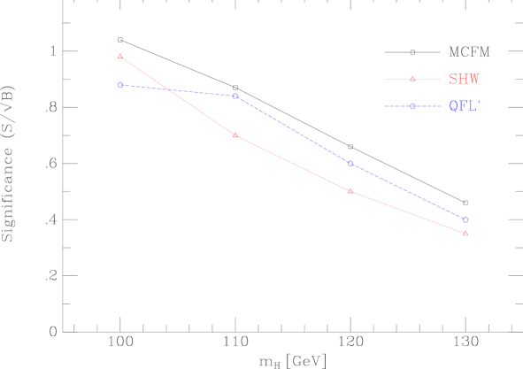
Figure 7: The significance obtained from our Monte Carlo MCFM, as presented in Table 4, compared to the results obtained by the SUSY-Higgs workshop [2]. Note that the MCFM significance should not be considered realistic because of the lack of detector effects.

The apparent similarity of the significances plotted in Fig. 7 is the result of two effects. We believe that the significance of ref. [2] is too high because, the $Zb\bar{b}$ and $ZZ$ backgrounds are underestimated in the light of the work presented here and in Ref. [15]. On the other hand, our significances are certainly too high, because due to the lack of a full detector simulation, the backgounds from processes with mis-identified leptons are underestimated.

4 Conclusions

We have presented the first results on the strong radiative corrections to the $Zb\bar{b}$ process. The results indicate large radiative corrections which can significantly change the estimates of the backgrounds to the process $p\bar{p}\rightarrow ZH$ at the Tevatron. We find that the significance $S/\sqrt{B}$ could be less than the result in the report of the SUSY-Higgs working group. The results described in this paper do not represent a full analysis of the potential to see the Higgs signature in the $ZH$ channel at the Tevatron. The most significant shortcoming is the lack of a full detector simulation.

The primary change is the increase in the size of the $Zb\bar{b}$-background because of the inclusion of NLO effects. Our calculation underscores the importance of having an experimental determination of the $Zb\bar{b}$ background, either by relating it to observed $Zb\bar{b}$ events at lower $m_{b\bar{b}}$ or by relating it to $Z$+two jet events.

Acknowledgements

This work was supported in part by the U.S. Department of Energy under Contract No. DE-AC02-76CH03000.

Appendix A Dipole formulae

This appendix details the exact dipole functions that we have used in the subtraction of the real integral, as well as the integrals of these dipoles that must be added to the loop contributions. We note that these functions differ slightly from those given in [5] since they carry no colour factors. In addition, these are the dipoles appropriate for the four-dimensional helicity scheme, which is the scheme of choice for the calculation of complicated virtual corrections. There are four basic types of dipole, corresponding to each of the emitter and spectator partons being in either the initial or final state. In all cases we label the partons as $\widetilde{ik}$ emitting parton $k$ with respect to the spectator $j$.

A.1 Initial-initial

We consider the case of an emitter $i$ and a spectator $j$, both in the initial state, radiating parton $k$ into the final state. We first define the dimensionless variable $x$ to be,

$$x=1-\frac{s_{ik}+s_{jk}}{s_{ij}}.$$ (19)

The dipole functions are then given by,

$${\cal D}_{ii,\,qq}^{ik,j} = \frac{g^{2}\mu^{2\epsilon}}{xp_{i}\cdot p_{k}}\left(\frac{2}{1-x}-1-x\right)$$

$${\cal D}_{ii,\,gq}^{ik,j} = \frac{g^{2}\mu^{2\epsilon}}{xp_{i}\cdot p_{k}}\left(x\right)$$

$${\cal D}_{ii,\,qg}^{ik,j} = \frac{g^{2}\mu^{2\epsilon}}{xp_{i}\cdot p_{k}}\left(1-2x(1-x)\right)$$

$${\cal D}_{ii,\,gg}^{ik,j} = \frac{g^{2}\mu^{2\epsilon}}{xp_{i}\cdot p_{k}}\left(\frac{2x}{1-x}+2x(1-x)\right)$$ (20)

These are the dipole functions if we neglect spin correlations between partons $i$ and $k$ and are thus not sufficient for the cases ${\cal D}_{ii,\,gq}$ and ${\cal D}_{ii,\,gg}$. If the lowest-order amplitude is represented by ${\cal M}_{\mu}$ (${\cal M}_{\nu}^{*}$), where $\mu$ ($\nu$) is the polarization index of gluon $\widetilde{ik}$, then the required subtraction is actually,

$$\left(-g^{\mu\nu}{\cal D}^{ik,j}+q^{\mu}q^{\nu}\,\widetilde{{\cal D}}^{ik,j}\right){\cal M}_{\mu}{\cal M}_{\nu}^{*},$$ (21)

where the additional pieces are,

$$\widetilde{{\cal D}}_{ii,\,gq}^{ik,j} = \frac{g^{2}\mu^{2\epsilon}}{xp_{i}\cdot p_{k}}\;\frac{1-x}{x}\frac{2p_{i}\cdot p_{j}}{p_{i}\cdot p_{k}\,p_{j}\cdot p_{k}},$$

$$\widetilde{{\cal D}}_{ii,\,gg}^{ik,j} = \widetilde{{\cal D}}_{ii,\,gq}^{ik,j},$$

$$q^{\mu} = p_{k}^{\mu}-\frac{p_{i}\cdot p_{k}}{p_{i}\cdot p_{j}}p_{j}^{\mu}.$$ (22)

When we perform the integration, it will be over the azimuthal average of these terms. The azimuthal average over the tensor $q^{\mu}q^{\nu}$ can only depend on the vectors $p_{i}$ and $p_{j}$ and since $q\cdot p_{i}=0$ it is equal to

$$\langle q^{\mu}q^{\nu}\rangle=A\Big{[}-g^{\mu\nu}+\frac{p_{i}^{\mu}p_{j}^{\nu}+p_{j}^{\mu}p_{i}^{\nu}}{p_{i}\cdot p_{j}}\Big{]}+Bp_{i}^{\mu}p_{i}^{\nu}$$ (23)

where $A=-q^{2}/2$. The final result is,

$$\langle{\cal D}^{ik,j}\rangle={\cal D}^{ik,j}-\frac{q^{2}}{2}\widetilde{{\cal D}}^{ik,j},$$ (24)

with $\widetilde{{\cal D}}_{ii,\,qq}=\widetilde{{\cal D}}_{ii,\,qg}=0$.

To integrate these dipoles we decompose the $n$-particle phase space in $d=4-2\epsilon$ dimensions,

$$d\phi^{(n)}(p_{a},p_{b}\rightarrow p_{1}\ldots p_{n})=\prod_{i=1,n}\;\Big{[}\frac{d^{d}p_{i}}{(2\pi)^{d-1}}\,\delta^{+}(p_{i}^{2})\Big{]}\;\;(2\pi)^{d}\,\delta^{(d)}(p_{a}+p_{b}-\sum_{i=1}^{n}p_{i})\;,$$ (25)

into two pieces,

$$d\phi^{(n)}(p_{i},p_{j}\rightarrow\ldots,k_{n-1},p_{k})=\int_{0}^{1}dx\;d\phi^{(n-1)}({\widetilde{p}}_{i},{\widetilde{p}}_{j}\rightarrow\ldots,{\widetilde{k}}_{n-1})\;\left[dp_{k}(p_{i},p_{j},x)\right]\;,$$ (26)

The first term corresponds to an $(n-1)$-particle phase-space and the second is the one-particle dipole sub-space that we must integrate over. Under this decomposition, the momenta of the particles are transformed. The final state momenta all undergo a Lorentz transformation (the details, which are given in ref. [5] erratum, are unimportant here), The initial momenta are modified with $p_{i}\to\widetilde{p}_{i}=xp_{i}$ and $p_{j}=\widetilde{p}_{j}$ is unchanged. The emitted parton phase space is given by,

$$\left[dp_{k}(p_{i},p_{j},x)\right]=\frac{d^{d}p_{k}}{(2\pi)^{d-1}}\,\delta^{+}(p_{k}^{2})\;\Theta(x)\Theta(1-x)\;$$ (27)

Eq. (27) can be rewritten as,

$$\left[dp_{k}(p_{i},p_{j},x)\right] = \frac{(2p_{i}p_{j})^{1-\epsilon}}{16\pi^{2}}\;\frac{d\Omega_{d-3}}{(2\pi)^{1-2\epsilon}}\;dv\;dx\;\Theta(x(1-x))\;\Theta(v)\;\Theta\!\left(1-\frac{v}{1-x}\right)$$ (28)

$$\times \;\left(1-x\right)^{-2\epsilon}\;\left[\frac{v}{1-x}\left(1-\frac{v}{1-x}\right)\right]^{-\epsilon}\;,$$

where $x$ is defined in Eq. (19), $v=p_{i}p_{k}/p_{i}p_{j}$ and $d\Omega_{d-3}$ is an element of solid angle in the directions perpendicular to the plane defined by $p_{i}$ and $p_{j}$.

$$\int\frac{d\Omega_{d-3}}{(2\pi)^{1-2\epsilon}}=\frac{(4\pi)^{\epsilon}}{\Gamma(1-\epsilon)}=c_{\Gamma}\;\;.$$ (29)

Isolating the common factor $g^{2}/p_{i}\cdot p_{k}$ from the dipole terms and re-writing all the momenta in terms of the transformed ones, we can further express this as,

$$\frac{g^{2}}{p_{i}\cdot p_{k}}\,[dp_{k}(p_{i},p_{j},x)]=\frac{d\Omega_{d-3}}{(2\pi)^{1-2\epsilon}}\,\frac{\alpha_{S}}{2\pi}\left(\frac{x}{2\widetilde{p}_{i}\cdot\widetilde{p}_{j}}\right)^{\epsilon}(1-x)^{-2\epsilon}\,\frac{dv}{v}\,\left(\frac{v}{1-x}\right)^{-\epsilon}\left(1-\frac{v}{1-x}\right)^{-\epsilon}.$$ (30)

This is now in a form where we can integrate the dipoles in Eq. (20). We perform the integrals and then expand in powers of $\epsilon$, discarding terms of $\cal{O}(\epsilon)$. In this way we find,

$$\int\,\left[dp_{k}(p_{i},p_{j},x)\right]\left[x\langle{\cal D}_{ii}^{ik,j}\rangle\right]=\left(\frac{\alpha_{S}}{2\pi}\right)\left(\frac{x\mu^{2}}{2\widetilde{p}_{i}\cdot\widetilde{p}_{j}}\right)^{\epsilon}\times c_{\Gamma}\Biggl{[}$$ (31)

$$-\frac{1}{\epsilon}\,p_{qq}(x)+\delta(1-x)\left(\frac{1}{\epsilon^{2}}+\frac{3}{2\epsilon}-\frac{\pi^{2}}{6}\right)+\frac{4\ln(1-x)}{(1-x)_{+}}-2(1+x)\ln(1-x)\Biggr{]},$$

where we have expressed the result in terms of the splitting function,

$$p_{qq}(x)=\frac{2}{(1-x)_{+}}-1-x+\frac{3}{2}\delta(1-x).$$ (32)

Before proceeding further we must perform mass factorization to get into the $\overline{MS}$ scheme. In $d=4-2\epsilon$ dimensions, the splitting functions contain additional terms

$$p_{ij}(x,\epsilon)=p_{ij}(x)+\epsilon\;p_{ij}^{(\epsilon)}(x)$$ (33)

We have the following expressions for the $p_{ij}$,

$$p_{qq}(x) = \frac{2}{(1-x)}_{+}-1-x+\frac{3}{2}\delta(1-x)+\epsilon\Big{(}-(1-x)+\frac{1}{2}\,\delta(1-x)\Big{)}\;,$$

$$p_{gq}(x) = \frac{1+(1-x)^{2}}{x}-\epsilon\;x\;,$$

$$p_{qg}(x) = x^{2}+(1-x)^{2}-\epsilon\;2x(1-x)\;,$$

$$p_{gg}^{(}x) = \frac{2}{(1-x)}_{+}+\frac{2}{x}-4+2x(1-x)+\delta(1-x)\left(\frac{11-2n_{f}/N}{6}\right)\;.$$ (34)

In order to arrive at the $\overline{MS}$ scheme, starting from results in the four-dimensional helicity scheme given by Eq. (31), we must subtract the counterterm

$$\left(\frac{\alpha_{S}}{2\pi}\right)\left[-\frac{1}{\epsilon}p_{qq}(x)+p_{qq}^{(\epsilon)}(x)\right]\;.$$ (35)

After performing this subtraction we have,

$$\left(\frac{\alpha_{S}}{2\pi}\right)\left\{\left(\frac{x\mu^{2}}{2\widetilde{p}_{i}\cdot\widetilde{p}_{j}}\right)^{\epsilon}\left[-\frac{1}{\epsilon}\,p_{qq}(x)+\ldots\right]-\left[-\frac{1}{\epsilon}\,p_{qq}(x)+p_{qq}^{(\epsilon)}(x)\right]\right\}$$ (36)

$$= \left(\frac{\alpha_{S}}{2\pi}\right)\left\{\left(\frac{x\mu^{2}}{2\widetilde{p}_{i}\cdot\widetilde{p}_{j}}\right)^{\epsilon}\biggl{[}\,\ldots\,\biggr{]}-(\ln x-L)p_{qq}(x)-p_{qq}^{(\epsilon)}(x)\right\},$$

where $\left[\ldots\right]$ represents all the non-$p_{qq}$ terms in Eq. (31). We have used the shorthand $L\equiv\ln(2\widetilde{p}_{i}\cdot\widetilde{p}_{j}/\mu^{2})$. With the above mass factorization procedure understood, we now introduce the notation,

$$\int\,\left[dp_{k}(p_{i},p_{j},x)\right]\left[x\langle{\cal D}_{ii}^{ik,j}\rangle\right]\equiv\left(\frac{\alpha_{S}}{2\pi}\right)\,c_{\Gamma}\;\left[{\cal V}_{ii}^{end}\delta(1-x)+{\cal V}_{ii}^{reg}+{\cal V}_{ii}^{plus}\right],$$ (37)

where we have split the result into an end-point contribution proportional to $\delta(1-x)$, regular terms and a term containing ‘plus’-distributions. In the $q\to q$ case we have,

$${\cal V}_{ii,\,qq}^{end} = \frac{1}{\epsilon^{2}}+\frac{1}{\epsilon}\left(\frac{3}{2}-L\right)+\frac{L^{2}}{2}-\frac{1}{2}-\frac{\pi^{2}}{6},$$

$${\cal V}_{ii,\,qq}^{reg} = 1-x-\frac{1+x^{2}}{1-x}\ln x-(1+x)\left(L+2\ln(1-x)\right),$$

$${\cal V}_{ii,\,qq}^{plus} = \frac{2L}{(1-x)_{+}}+4\Bigg{[}\frac{\ln(1-x)}{1-x}\Bigg{]}_{+}.$$ (38)

The expressions for the other parton splittings, derived in the same manner are,

$${\cal V}_{ii,\,qg}^{end} = {\cal V}_{ii,\,qg}^{plus}\,=\,0,$$

$${\cal V}_{ii,\,qg}^{reg} = (1-2x(1-x))(L-\ln x+2\ln(1-x))+2x(1-x),$$

$${\cal V}_{ii,\,gq}^{end} = {\cal V}_{ii,\,gq}^{plus}\,=\,0,$$

$${\cal V}_{ii,\,gq}^{reg} = \left(\frac{1+(1-x)^{2}}{x}\right)(L-\ln x+2\ln(1-x))+x,$$

$${\cal V}_{ii,\,gg}^{end} = \frac{1}{\epsilon^{2}}-\frac{L}{\epsilon}+\frac{L^{2}}{2}-\frac{\pi^{2}}{6}+\frac{1}{6\epsilon}\left(11-\frac{2n_{f}}{N}\right),$$

$${\cal V}_{ii,\,gg}^{reg} = 2(L-\ln x+2\ln(1-x))\left(\frac{1-x}{x}+x(1-x)-1\right)-\frac{2\ln x}{1-x},$$

$${\cal V}_{ii,\,gg}^{plus} = \frac{2L}{(1-x)_{+}}+4\Bigg{[}\frac{\ln(1-x)}{1-x}\Bigg{]}_{+}.$$ (39)

A.2 Initial-final

We now consider the case of an initial emitter $i$ with respect to a final state spectator $j$. We first define the dimensionless variables $x$ and $u$ to be,

$$x=1-\frac{s_{jk}}{s_{ik}+s_{ij}},\qquad u=\frac{s_{ik}}{s_{ik}+s_{ij}}.$$ (40)

The dipole functions are then given by,

$${\cal D}_{if,\,qq}^{ik,j} = \frac{g^{2}\mu^{2\epsilon}}{xp_{i}\cdot p_{k}}\left(\frac{2}{1-x+u}-1-x\right),$$

$${\cal D}_{if,\,gq}^{ik,j} = \frac{g^{2}\mu^{2\epsilon}}{xp_{i}\cdot p_{k}}\left(x\right),$$

$${\cal D}_{if,\,qg}^{ik,j} = \frac{g^{2}\mu^{2\epsilon}}{xp_{i}\cdot p_{k}}\left(1-2x(1-x)\right),$$

$${\cal D}_{if,\,gg}^{ik,j} = \frac{g^{2}\mu^{2\epsilon}}{xp_{i}\cdot p_{k}}\left(\frac{2}{1-x+u}-2+2x(1-x)\right),$$ (41)

with the additional variables needed to account for spin correlations,

$$\widetilde{{\cal D}}_{if,\,gq}^{ik,j} = \frac{g^{2}\mu^{2\epsilon}}{xp_{i}\cdot p_{k}}\,\frac{2(1-x)}{x}\,\frac{u(1-u)}{p_{j}\cdot p_{k}},$$

$$\widetilde{{\cal D}}_{if,\,gg}^{ik,j} = \widetilde{{\cal D}}_{if,\,gq}^{ik,j},$$

$$q^{\mu} = \frac{p_{k}^{\mu}}{u}-\frac{p_{j}^{\mu}}{1-u}.$$ (42)

The phase-space convolution becomes

$$d\phi^{(n)}(p_{i},p_{b}\rightarrow\ldots,p_{j},p_{k})=\int_{0}^{1}dx\;d\phi^{(n-1)}(\widetilde{p}_{i},p_{b}\rightarrow\ldots,{\widetilde{p}}_{j})\;\left[dp_{k}({\widetilde{p}}_{j};p_{i},x)\right]\;,$$ (43)

where the transformed momenta $\widetilde{p}_{i}$ and $\widetilde{p}_{j}$ are defined in terms of the original momenta by,

$$\widetilde{p}_{i}=xp_{i},\qquad\widetilde{p}_{j}=p_{j}+p_{k}+(1-x)p_{i},$$ (44)

and $\widetilde{p}_{i}^{2}=\widetilde{p}_{j}^{2}=0$. The dipole phase space is,

$$\left[dp_{k}({\widetilde{p}}_{j};p_{i},x)\right]=\frac{d^{d}p_{k}}{(2\pi)^{d-1}}\,\delta^{+}(p_{k}^{2})\;\Theta(x)\Theta(1-x)\;\frac{1}{1-u}\;\;.$$ (45)

Using the kinematic variables in Eq. (40), the phase space in Eq. (45) can be written as follows

$$\left[dp_{k}({\widetilde{p}}_{j};p_{i},x)\right] = \frac{(2{\widetilde{p}}_{j}p_{i})^{1-\epsilon}}{16\pi^{2}}\;\frac{d\Omega_{d-3}}{(2\pi)^{1-2\epsilon}}\;du\;dx\;\Theta(u(1-u))\;\Theta(x(1-x))$$ (46)

$$\cdot \;\left(u(1-u)\right)^{-\epsilon}\;\left(1-x\right)^{-\epsilon}\;$$

where $d\Omega_{d-3}$ is an element of solid angle perpendicular to ${\widetilde{p}}_{k}$ and $p_{1}$.

We manipulate further as before to yield,

$$\frac{g^{2}}{p_{i}\cdot p_{k}}\,\left[dp_{k}({\widetilde{p}}_{j};p_{i},x)\right]=\frac{d\Omega_{d-3}}{(2\pi)^{1-2\epsilon}}\,\frac{\alpha_{S}}{2\pi}\left(\frac{x}{2\widetilde{p}_{i}\cdot\widetilde{p}_{j}}\right)^{\epsilon}(1-x)^{-\epsilon}du\,u^{-1-\epsilon}(1-u)^{-\epsilon}.$$ (47)

The integration of the dipoles with this phase space and the mass factorization procedure are handled in the same way as the initial-initial case detailed above. The only challenging integral is given by

$$I_{if} = \int_{0}^{1}du\;u^{-1-\epsilon}(1-u)^{-\epsilon}\frac{1}{(1-x+u)}$$ (48)

$$= -\frac{1}{\epsilon}\frac{\Gamma^{2}(1-\epsilon)}{\Gamma(1-2\epsilon)}\frac{(2-x)^{\epsilon}}{(1-x)^{1+\epsilon}}\;F(-\epsilon,-2\epsilon;1-2\epsilon;\frac{1}{2-x})$$

where $F(-\epsilon,-2\epsilon;1-2\epsilon;\frac{1}{2-x})=1+{\cal O}(\epsilon^{2}(1-x)^{0})$. Making the separation of the integrated dipoles into different types of contribution yields, (in a notation similar to Eq. (37)).

$${\cal V}_{if,\,qq}^{end} = \frac{1}{\epsilon^{2}}+\frac{1}{\epsilon}\left(\frac{3}{2}-L\right)+\frac{L^{2}}{2}-\frac{1}{2}+\frac{\pi^{2}}{6},$$

$${\cal V}_{if,\,qq}^{reg} = 1-x-\frac{2\ln(2-x)}{1-x}-(1+x)\left(L-\ln x+\ln(1-x)\right)-\frac{2\ln x}{1-x},$$

$${\cal V}_{if,\,qq}^{plus} = \frac{2L}{(1-x)_{+}}+4\Bigg{[}\frac{\ln(1-x)}{1-x}\Bigg{]}_{+}.$$

$${\cal V}_{if,\,qg}^{end} = {\cal V}_{if,\,qg}^{plus}\,=\,0,$$

$${\cal V}_{if,\,qg}^{reg} = (1-2x(1-x))(L-\ln x+\ln(1-x))+2x(1-x),$$

$${\cal V}_{if,\,gq}^{end} = {\cal V}_{if,\,gq}^{plus}\,=\,0,$$

$${\cal V}_{if,\,gq}^{reg} = \left(\frac{1+(1-x)^{2}}{x}\right)(L-\ln x+\ln(1-x))+x,$$

$${\cal V}_{if,\,gg}^{end} = \frac{1}{\epsilon^{2}}-\frac{L}{\epsilon}+\frac{L^{2}}{2}+\frac{\pi^{2}}{6}+\frac{1}{6\epsilon}\left(11-\frac{2n_{f}}{N}\right),$$

$${\cal V}_{if,\,gg}^{reg} = 2(L-\ln x+\ln(1-x))\left(\frac{1-x}{x}+x(1-x)-1\right)-\frac{2\ln(2-x)}{1-x}-\frac{2\ln x}{1-x},$$

$${\cal V}_{if,\,gg}^{plus} = \frac{2L}{(1-x)_{+}}+4\Bigg{[}\frac{\ln(1-x)}{1-x}\Bigg{]}_{+}.$$ (49)

A.3 Final-initial

We now consider a final state emitter $i$, with respect to an initial state spectator $j$. We first define the dimensionless variables $x$ and $z$ to be,

$$x=1-\frac{s_{ik}}{s_{ij}+s_{jk}},\qquad z=\frac{s_{ij}}{s_{ij}+s_{jk}}.$$ (50)

The dipole functions are then given by,

$${\cal D}_{fi,\,qq}^{ik,j} = \frac{g^{2}\mu^{2\epsilon}}{xp_{i}\cdot p_{k}}\left(\frac{2}{1-x+1-z}-1-z\right),$$

$${\cal D}_{fi,\,gq}^{ik,j} = \frac{g^{2}\mu^{2\epsilon}}{xp_{i}\cdot p_{k}},$$

$${\cal D}_{fi,\,gg}^{ik,j} = \frac{g^{2}\mu^{2\epsilon}}{xp_{i}\cdot p_{k}}\left(\frac{2}{1-x+1-z}+\frac{2}{1-x+z}-4\right),$$ (51)

There is no dipole ${\cal D}_{fi,\,qg}$ since the singularities are already accounted for by ${\cal D}_{fi,\,qq}$. The dipole pieces associated with spin correlations are given by,

$$\widetilde{{\cal D}}_{fi,\,gq}^{ik,j} = \frac{g^{2}\mu^{2\epsilon}}{xp_{i}\cdot p_{k}}\,\frac{-2}{p_{i}\cdot p_{k}},$$

$$\widetilde{{\cal D}}_{fi,\,gg}^{ik,j} = -\widetilde{{\cal D}}_{fi,\,gq}^{ik,j},$$

$$q^{\mu} = zp_{i}^{\mu}-(1-z)p_{k}^{\mu}.$$ (52)

The phase-space has the following convolution structure,

$$d\phi^{(n)}(p_{a},p_{j}\rightarrow\ldots,p_{i},p_{k})=\int_{0}^{1}dx\;d\phi^{(n-1)}(p_{a},xp_{j},\rightarrow\ldots,\widetilde{p}_{ik})\;\left[dp_{k}({\widetilde{p}}_{i};p_{j},x)\right]\;,$$ (53)

where

$$\left[dp_{k}({\widetilde{p}}_{i};p_{j},x)\right]=\frac{d^{d}p_{k}}{(2\pi)^{d-1}}\,\delta^{+}(p_{k}^{2})\;\Theta(x)\Theta(1-x)\;\frac{1}{1-z}\;\;,$$ (54)

and the transformed momenta are given by,

$$\widetilde{p}_{i} = p_{i}+p_{k}+(1-x)p_{j}$$

$$\widetilde{p}_{j} = xp_{j}.$$ (55)

Equation (54) can be written out more explicitly as,

$$\left[dp_{k}({\widetilde{p}}_{i};p_{j},x)\right] = \frac{(2{\widetilde{p}}_{i}p_{j})^{1-\epsilon}}{16\pi^{2}}\;\frac{d\Omega_{d-3}}{(2\pi)^{1-2\epsilon}}\;dz\;dx\;\Theta(z(1-z))\;\Theta(x(1-x))$$ (56)

$$\times \;\left(z(1-z)\right)^{-\epsilon}\;\left(1-x\right)^{-\epsilon}\;,$$

where $d\Omega_{d-3}$ is an element of solid angle perpendicular to the plane defined by ${\widetilde{p}}_{i}$ and $p_{j}$.

The form needed to integrate the dipoles is then,

$$\frac{g^{2}}{p_{i}\cdot p_{k}}\,[dp_{k}(\widetilde{p}_{ik};p_{j},x)]=\frac{d\Omega_{d-3}}{(2\pi)^{1-2\epsilon}}\,\frac{\alpha_{S}}{2\pi}\left(\frac{x}{2\widetilde{p}_{i}\cdot\widetilde{p}_{j}}\right)^{\epsilon}(1-x)^{-1-\epsilon}dz\,z^{-\epsilon}(1-z)^{-\epsilon},$$ (57)

and the integrations over $z$ can now be performed. The only difficult integral is

$$I_{fi} = \int_{0}^{1}dz\;z^{-\epsilon}(1-z)^{-\epsilon}\frac{1}{(1-x+z)}=-\frac{1}{\epsilon}\frac{\Gamma^{2}(1-\epsilon)}{\Gamma(1-2\epsilon)}$$ (58)

$$\times\Bigg{[}(2-x)^{-2\epsilon}F(\epsilon,2\epsilon;1+\epsilon;\frac{1-x}{2-x})-\Big{(}(1-x)(2-x)\Big{)}^{-\epsilon}\frac{\Gamma(1-2\epsilon)\Gamma(1+\epsilon)}{\Gamma(1-\epsilon)}\Bigg{]}$$

where $F(\epsilon,2\epsilon;1+\epsilon;z)=1+O(\epsilon^{2}z)$. With definitions analogous to Eq. (37) we find,

$${\cal V}_{fi,\,qq}^{end} = \frac{1}{\epsilon^{2}}+\frac{1}{\epsilon}\left(\frac{3}{2}-L\right)+\frac{L^{2}}{2}-\frac{3L}{2}+3-\frac{\pi^{2}}{2},$$

$${\cal V}_{fi,\,qq}^{reg} = \frac{2\ln(2-x)}{1-x},$$

$${\cal V}_{fi,\,qq}^{plus} = -\Bigg{[}\frac{2\ln(1-x)}{(1-x)}\Bigg{]}_{+}-\frac{3}{2(1-x)_{+}}.$$

$${\cal V}_{fi,\,gq}^{end} = -\frac{2}{3\epsilon}-\frac{13}{9}+\frac{2L}{3},$$

$${\cal V}_{fi,\,gq}^{reg} = 0,$$

$${\cal V}_{fi,\,gq}^{plus} = \frac{2}{3}\,\frac{1}{(1-x)_{+}},$$

$${\cal V}_{fi,\,gg}^{end} = \frac{2}{\epsilon^{2}}+\frac{1}{\epsilon}(\frac{11}{3}-2L)-\frac{11L}{3}+L^{2}+\frac{67}{9}-\pi^{2},$$

$${\cal V}_{fi,\,gg}^{reg} = \frac{4\ln(2-x)}{1-x},$$

$${\cal V}_{fi,\,gg}^{plus} = -\Bigg{[}\frac{4\ln(1-x)}{1-x}\Bigg{]}_{+}-\frac{11}{3(1-x)_{+}}.$$ (59)

A.4 Final-final

The remaining dipole to consider is one in which we have a final state emitter $i$ with respect to a final state spectator $j$. In this case we define the dimensionless variables $y$ and $z$,

$$y=\frac{s_{ik}}{s_{ik}+s_{ij}+s_{jk}},\qquad z=\frac{s_{ij}}{s_{ij}+s_{jk}}.$$ (60)

The dipole functions are then given by,

$${\cal D}_{ff,\,qq}^{ik,j} = \frac{g^{2}\mu^{2\epsilon}}{p_{i}\cdot p_{k}}\left(\frac{2}{1-z(1-y)}-1-z\right),$$

$${\cal D}_{ff,\,gq}^{ik,j} = \frac{g^{2}\mu^{2\epsilon}}{p_{i}\cdot p_{k}},$$

$${\cal D}_{ff,\,gg}^{ik,j} = \frac{g^{2}\mu^{2\epsilon}}{p_{i}\cdot p_{k}}\left(\frac{2}{1-z(1-y)}+\frac{2}{1-(1-z)(1-y)}-4\right),$$ (61)

with the auxiliary information,

$$\widetilde{{\cal D}}_{ff,\,gq}^{ik,j} = \frac{g^{2}\mu^{2\epsilon}}{p_{i}\cdot p_{k}}\,\frac{-2}{p_{i}\cdot p_{k}},$$

$$\widetilde{{\cal D}}_{ff,\,gg}^{ik,j} = -\widetilde{{\cal D}}_{ff,\,gq}^{ik,j},$$

$$q^{\mu} = zp_{i}^{\mu}-(1-z)p_{k}^{\mu}.$$ (62)

In terms of the momenta ${\widetilde{p}}_{i},\,{\widetilde{p}}_{j}$ and $p_{k}$, this phase-space contribution takes the factorized form:

$$d\phi^{(n)}(p_{a},p+b\rightarrow\ldots,p_{i},p_{k},p_{j})=d\phi^{(n-1)}(p_{a},p+b\rightarrow\ldots,{\widetilde{p}}_{i},{\widetilde{p}}_{j})\left[dp_{k}({\widetilde{p}}_{i},{\widetilde{p}}_{j})\right]\;\;,$$ (63)

where

$$\left[dp_{k}({\widetilde{p}}_{i},{\widetilde{p}}_{j})\right]=\frac{d^{d}p_{k}}{(2\pi)^{d-1}}\,\delta^{+}(p_{k}^{2})\;{\cal J}(p_{k};{\widetilde{p}}_{i},{\widetilde{p}}_{j})\;,$$ (64)

and the Jacobian factor is

$${\cal J}(p_{k};{\widetilde{p}}_{i},{\widetilde{p}}_{j})=\Theta(1-z)\,\Theta(1-y)\;\frac{(1-y)^{d-3}}{1-z}\;.$$ (65)

In terms of the kinematic variables defined earlier, we have

$$\left[dp_{k}({\widetilde{p}}_{i},{\widetilde{p}}_{j})\right] = \frac{(2{\widetilde{p}}_{i}{\widetilde{p}}_{j})^{1-\epsilon}}{16\pi^{2}}\;\frac{d\Omega_{d-3}}{(2\pi)^{1-2\epsilon}}\;dz\;dy\;\Theta(z(1-z))\;\Theta(y(1-y))$$ (66)

$$\times \;\left(z(1-z)\right)^{-\epsilon}\;\left(1-y\right)^{1-2\epsilon}y^{-\epsilon}\;,$$

where $d\Omega_{d-3}$ is an element of solid angle perpendicular to ${\widetilde{p}}_{ij}$ and ${\widetilde{p}}_{k}$. In this case the momenta transform as,

$$\widetilde{p}_{i}=p_{i}+p_{k}-\left(\frac{y}{1-y}\right)\,p_{j},\qquad\widetilde{p}_{j}=\frac{1}{(1-y)}\,p_{j},$$ (67)

and the phase-space factorizes to yield the relevant measure,

$$\frac{g^{2}}{p_{i}\cdot p_{k}}\,[dp_{k}(\widetilde{p}_{i},\widetilde{p}_{j},x)]=\frac{d\Omega_{d-3}}{(2\pi)^{1-2\epsilon}}\,\frac{\alpha_{S}}{2\pi}\left(\frac{1}{2\widetilde{p}_{i}\cdot\widetilde{p}_{j}}\right)^{\epsilon}dz\,z^{-\epsilon}(1-z)^{-\epsilon}\,dy\,y^{-1-\epsilon}(1-y)^{1-2\epsilon}.$$ (68)

The soft integral is then given by

$$I_{ff} = \int_{0}^{1}dz\;z^{-\epsilon}(1-z)^{-\epsilon}\int_{0}^{1}dy\;y^{-1-\epsilon}(1-y)^{1-2\epsilon}\frac{1}{1-z(1-y)}$$ (69)

$$= \frac{1}{2\epsilon^{2}}\frac{\Gamma^{3}(1-\epsilon)}{\Gamma(1-3\epsilon)}$$

In this case, there is no need to separate the integrated forms of these dipoles and with the simplified notation,

$$\int\,[dp_{k}(\widetilde{p}_{i},\widetilde{p}_{j},x)]\left[\langle{\cal D}_{ff}^{ik,j}\rangle\right]\equiv\left(\frac{\alpha_{S}}{2\pi}\right)\,c_{\Gamma}\;{\cal V}_{ff},$$ (70)

we find,

$${\cal V}_{ff,\,qq} = \frac{1}{\epsilon^{2}}+\frac{1}{\epsilon}\left(\frac{3}{2}-L\right)+\frac{L^{2}}{2}-\frac{3L}{2}+\frac{9}{2}-\frac{\pi^{2}}{2},$$

$${\cal V}_{ff,\,gq} = -\frac{2}{3\epsilon}-\frac{19}{9}+\frac{2L}{3},$$

$${\cal V}_{ff,\,gg} = \frac{2}{\epsilon^{2}}+\frac{1}{\epsilon}\left(\frac{11}{3}-2L\right)+L^{2}-\frac{11L}{3}+\frac{100}{9}-\pi^{2}.$$ (71)

References

- [1] R.K. Ellis and Sinisa Veseli, Phys. Rev. D60 (011501) 1999; e-print archive: hep-ph/9810489.
-
[2]
A. Stange, W. Marciano and S. Willenbrock, Phys. Rev. D49 (1354)
1994; e-print archive: hep-ph/9309294
Susy-Higgs working group. - [3] Z. Nagy and Z. Trocsanyi, hep-ph/9806317, Phys. Rev.D59 (014020) 1999, Erratum July, 2000.
- [4] R. K. Ellis, D. A. Ross and A. E. Terrano, Nucl. Phys. B178, 421 (81).
- [5] S. Catani and M. H. Seymour, Nucl. Phys. B485, 291 (1997), Erratum ibid. B510, 503 (1997).
- [6] F.A. Berends and W. Giele, Nucl. Phys. B294, 700 (87).
- [7] For a review, see S Catani et al., hep-ph/0005025.
- [8] Z. Bern, L. Dixon and D. Kosower, Nucl. Phys. B513, 3 (1998).
-
[9]
E. W. N. Glover and D. J. Miller,
Phys. Lett. B396, 257 (1997);
Z. Bern, L. Dixon, D. Kosower and S. Weinzierl, Nucl. Phys. B489, 3 (1997);
J. M. Campbell, E. W. N. Glover and D. J. Miller, Phys. Lett. B409, 503 (1998). - [10] H. Georgi, Nucl. Phys. 363, 301 (1991).
- [11] A.D. Martin, R.G. Roberts, W.J. Stirling and R.S. Thorne, Euro. Phys. J. C4, 463 (1998), e-print archive: hep-ph/9803445.
- [12] W.M. Yao, FERMILAB-CONF-96-383-E, presented at 1996 DPF/DPB Summer Study on New Directions for High-energy Physics (Snowmass 96), Snowmass, CO, July 1996.
- [13] Discovering a light mass Higgs boson at the Tevatron collider, S. Mrenna, Publ. in: Perspectives on Higgs physics, 2nd ed. G L Kane World Sci., Singapore, 1997 Advanced Series on Directions in High-Energy Physics ; 17 (131-147).
-
[14]
A. Stange, W. Marciano and S. Willenbrock,
Phys. Rev. D49, 1354 (1994),
ibid. D50, 4491 (1994);
S. Kuhlmann, TeV2000 report. - [15] J.M. Campbell and R.K. Ellis, Phys. Rev. D60, 113006 (1999), e-print archive: hep-ph/9905386