PARTON DISTRIBUTIONS WORKING GROUP

Abstract

This report summarizes the activities of the Parton Distributions Working Group of the ’QCD and Weak Boson Physics workshop’ held in preparation for Run II at the Fermilab Tevatron. The main focus of this working group was to investigate the different issues associated with the development of quantitative tools to estimate parton distribution functions uncertainties. In the conclusion, we introduce a ”Manifesto” that describes an optimal method for reporting data.

INTRODUCTION

With Run II and its large increase in integrated luminosity, the Tevatron will enter an era of high precision measurements. In this era, parton distribution function (PDF) uncertainties will play a major role.

The basic questions for PDFs at the Tevatron Run II are simple and common to all other experiment:

• What limitations will the PDFs put on physics analysis?

• What information can we gain about the PDFs?

There are some qualitative tools that exists and can be used to try to answer these questions. However, beside S. Alekhin’s pioneer work [1], quantitative tools that attempt to include all sources of uncertainties are not available yet. The main focus of this working group has therefore been to investigate the different issues associated with the development of those tools, although obviously other topics have also been investigated.

We have divided this summary of activities into individual contributions:

• UNCERTAINTIES OF PARTON DISTRIBUTION FUNCTIONS AND THEIR IMPLICATION ON PHYSICAL PREDICTIONS. R. Brok et al. describe preliminary results from an effort to quantify the uncertainties in PDFs and the resulting uncertainties in predicted physical quantities. The production cross section of the W boson is given as a first example.

• PARTON DISTRIBUTION FUNCTION UNCERTAINTIES. Giele et al. review the status of their effort to extract PDFs from data with a quantitative estimate of the uncertainties.

• EXPERIMENTAL UNCERTAINTIES AND THEIR DISTRIBUTIONS IN THE INCLUSIVE JET CROSS SECTION. R. Hirosky summarizes the current CDF and D0 analysis for the inclusive jet cross sections. So far the uncertainties have been assumed to be Gaussian distributed. He investigates what information can be extracted about the shape of the uncertainties with the goal of being able to provide a way to calculate the Likelihood.

• PARTON DENSITY UNCERTAINTIES AND SUSY PARTICLE PRODUCTION. T. Plehn and M. Krämer study the current status of PDF’s uncertainties on SUSY particle mass bounds or mass determinations.

• SOFT-GLUON RESUMMATION AND PDF THEORY UNCERTAINTIES. G. Sterman and W. Vogelsang discuss the interplay of higher order corrections and PDF determinations, and the possible use of soft-gluon resummation in global fits.

• PARTON DISTRIBUTION FUNCTIONS: EXPERIMENTAL DATA AND THEIR INTERPRETATION. L. de Barbaro review current issues in the interpretation of experimental data and the outlook for future data.

• HEAVY QUARK PRODUCTION. Olness et al. present a status report of a variety of projects related to heavy quark production.

• PARTON DENSITIES FOR HEAVY QUARKS. J. Smith compares different PDFs for heavy quarks.

• CONSTRAINTS ON THE GLUON DENSITY FROM LEPTON PAIR PRODUCTION. E. L. Berger and M. Klasen study the sensitivity of the hadroproduction of lepton pairs to the gluon density.

Note that the individual references are at the end of the corresponding contribution. The references for the introduction and the conclusion are at the end.

UNCERTAINTIES OF PARTON DISTRIBUTION FUNCTIONS AND THEIR IMPLICATIONS ON PHYSICAL PREDICTIONS

R. Brock, D. Casey, J. Huston, J. Kalk, J. Pumplin, D. Stump, W.K. Tung

Department of Physics and Astronomy, Michigan State University, East Lansing, MI 48824

Abstract

We describe preliminary results from an effort to quantify the uncertainties in parton distribution functions and the resulting uncertainties in predicted physical quantities. The production cross section of the $W$ boson is given as a first example. Constraints due to the full data sets of the CTEQ global analysis are used in this study. Two complementary approaches, based on the Hessian and the Lagrange multiplier method respectively, are outlined. We discuss issues on obtaining meaningful uncertainty estimates that include the effect of correlated experimental systematic uncertainties and illustrate them with detailed calculations using one set of precision DIS data.

1 Introduction

Many measurements at the Tevatron rely on parton distribution functions (PDFs) for significant portions of their data analysis as well as the interpretation of their results. For example, in cross section measurements the acceptance calculation often relies on Monte Carlo (MC) estimates of the fraction of unobserved events. As another example, the measurement of the mass of the $W$ boson depends on PDFs via the modeling of the production of the vector boson in MC. In such cases, uncertainties in the PDFs contribute, by necessity, to uncertainties on the measured quantities. Critical comparisons between experimental data and the underlying theory are often even more dependent upon the uncertainties in PDFs. The uncertainties on the production cross sections for $W$ and $Z$ bosons, currently limited by the uncertainty on the measured luminosity, are approximately 4%. At this precision, any comparison with the theoretical prediction inevitably raises the question: How “certain” is the prediction itself?

A recent example of the importance of PDF uncertainty is the proper interpretation of the measurement of the high-$E_{T}$ jet cross-section at the Tevatron. When the first CDF measurement was published [1], there was a great deal of controversy over whether the observed excess, compared to theory, could be explained by deviations of the PDFs, especially the gluon, from the conventionally assumed behavior, or could it be the first signal for some new physics [2].

With the unprecedented precision and reach of many of the Run I measurements, understanding the implications of uncertainties in the PDFs has become a burning issue. During Run II (and later at LHC) this issue may strongly affect the uncertainty estimates in precision Standard Model studies, such as the all important $W$-mass measurement, as well as the signal and background estimates in searches for new physics.

In principle, it is the uncertainties on physical quantities due to parton distributions, rather than on the PDFs themselves, that is of primary concern. The latter are theoretical constructs which depend on the renormalization and factorization schemes; and there are strong correlations between PDFs of different flavors and from different values of $x$, which can compensate each other in the convolution integrals that relate them to physical cross-sections. On the other hand, since PDFs are universal, if we can obtain meaningful estimates of their uncertainties based on analysis of existing data, then the results can be applied to all processes that are of interest in the future. [3, 4]

One can attempt to assess directly the uncertainty on a specific physical prediction due to the full range of PDFs allowed by available experimental constraints. This approach will provide a more reliable estimate for the range of possible predictions for the physical variable under study, and may be the best course of action for ultra-precise measurements such as the mass of the $W$ boson or the $W$ production cross-section. However, such results are process-specific and therefore the analysis must be carried out for each case individually.

Until recently, the attempts to quantify either the uncertainties on the PDFs themselves (via uncertainties on their functional parameters, for instance) or the uncertainty on derived quantities due to variations in the PDFs have been rather unsatisfactory. Two commonly used methods are: (1) Comparing the predictions obtained with different PDF sets, e.g., various CTEQ [5], MRS [6] and GRV [7] sets; (2)

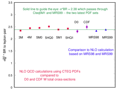
Figure 1: Predicted cross section for $W$ boson production for various PDFs.

Within a given global analysis effort, varying individual functional parameters ad hoc, within limits considered to be consistent with the existing data, e.g. [8]. Neither method provides a systematic, quantitative measure of the uncertainties of the PDFs or their predictions.

As a case in point, Fig. 1 shows how the calculated value of the cross section for $W$ boson production at the Tevatron varies with a set of historical CTEQ PDFs as well as the most recent CTEQ [5] and MRST [6] sets. Also shown are the most recent measurements from DØ and CDF. While it is comforting to see that the predictions have remained within a narrow range, the variation observed cannot be characterized as a meaningful estimate of the uncertainty: (i) the variation with time reflects mostly the changes in experimental input to, or analysis procedure of, the global analyses; and (ii) the perfect agreement between the values of the most recent CTEQ5M1  and MRS99 sets must be fortuitous, since each group has also obtained other satisfactory sets which give rise to much larger variations of the $W$ cross section. The MRST group, in particular has examined the range of this variation by setting a variety of parameters to some extreme values [8]. These studies are useful but can not be considered quantitative or definitive. What is needed are methods that explore thoroughly the possible variations of the parton distribution functions.

It is important to recognize all potential sources of uncertainty in the determination of PDFs. Focusing on some of these, while neglecting significant others, may not yield practically useful results. Sources of uncertainty are listed below:

• Statistical uncertainties of the experimental data used to determine the PDFs. These vary over a wide range among the experiments used in a global analysis, but are straightforward to treat.

• Systematic uncertainties within each data set. There are typically many sources of experimental systematic uncertainty, some of which are highly correlated. These uncertainties can be treated by standard methods of probability theory provided they are precisely known, which unfortunately is often not the case – either because they may not be randomly distributed and/or because their estimation in practice involves subjective judgements.

• Theoretical uncertainties arising from higher-order PQCD corrections, resummation corrections near the boundaries of phase space, power-law (higher twist) and nuclear target corrections, etc.

• Uncertainties due to the parametrization of the non-perturbative PDFs, $f_{a}(x,Q_{0})$, at some low momentum scale $Q_{0}$. The specific choice of the functional form used at $Q_{0}$ introduces implicit correlations between the various $x$-ranges, which could be as important, if not more so, than the experimental correlations in the determination of $f_{a}(x,Q)$ for all $Q$.

Since strict quantitative statistical methods are based on idealized assumptions, such as random measurement uncertainties, an important trade-off must be faced in devising a strategy for the analysis of PDF uncertainties. If emphasis is put on the “rigor” of the statistical method, then many important experiments cannot be included in the analysis, either because the published errors appear to fail strict statistical tests or because data from different experiments appear to be mutually exclusive in the parton distribution parameter space [4]. If priority is placed on using the maximal experimental constraints from available data, then standard statistical methods may not apply, but must be supplemented by physical considerations, taking into account experimental and theoretical limitations. We choose the latter tack, pursuing the determination of the uncertainties in the context of the current CTEQ global analysis. In particular, we include the same body of the world’s data as constraints in our uncertainty study as that used in the CTEQ5 analysis; and adopt the “best fit” – the CTEQ5M1 set – as the base set around which the uncertainty studies are performed. In practice, there are unavoidable choices (and compromises) that must be made in the analysis. (Similar subjective judgements often are also necessary in estimating certain systematic errors in experimental analyses.) The most important consideration is that quantitative results must remain robust with respect to reasonable variations in these choices.

In this Report we describe preliminary results obtained by our group using the two approaches mentioned earlier. In Section 3 we focus on the error matrix, which characterizes the general uncertainties of the non-perturbative PDF parameters. In Sections 4 and 5 we study specifically the production cross section $\sigma_{W}$ for $W^{\pm}$ bosons at the Tevatron, to estimate the uncertainty of the prediction of $\sigma_{W}$ due to PDF uncertainty. We start in Section 2 with a review of some aspects of the CTEQ global analysis on which this study is based.

2 Elements of the Base Global Analysis

Since our strategy is based on using the existing framework of the CTEQ global analysis, it is useful to review some of its features pertinent to the current study [5].

Data selection:

Table 1 shows the experimental data sets included in the CTEQ5 global analysis, and in the current study. For neutral current DIS data only the most accurate proton and deuteron target measurements are kept, since they are the “cleanest” and they are already extremely extensive. For charged current (neutrino) DIS data, the significant ones all involve a heavy (Fe) target. Since these data are crucial for the determination of the normalization of the gluon distribution (indirectly via the momentum sum rule), and for quark flavor differentiation (in conjunction with the neutral current data), they play an important role in any comprehensive global analysis. For this purpose, a heavy-target correction is applied to the data, based on measured ratios for heavy-to-light targets from NMC and other experiments. Direct photon production data are not included because of serious theoretical uncertainties, as well as possible inconsistencies between existing experiments. Cf. [5] and [9]. The combination of neutral and charged DIS, lepton-pair production, lepton charge asymmetry, and inclusive large-$p_{T}$ jet production processes provides a fairly tightly constrained system for the global analysis of PDFs. In total, there are $\sim$1300 data points which meet the minimum momentum scale cuts which must be imposed to ensure that PQCD applies. The fractional uncertainties on these points are distributed roughly like $dF/F$ over the range $F=0.003-0.4$.

Process	Experiment	Measurable	$N_{data}$
DIS	BCDMS[10]	$F_{2\ H}^{\mu},F_{2\ D}^{\mu}$	324
	NMC [11]	$F_{2\ H}^{\mu},F_{2\ D}^{\mu}$	240
	H1 [12]	$F_{2\ H}^{e}$	172
	ZEUS[13]	$F_{2\ H}^{e}$	186
	CCFR [14]	$F_{2\ Fe}^{\nu},x\ F_{3\ Fe}^{\nu}$	174
Drell-Yan	E605[15]	$sd\sigma/d\sqrt{\tau}dy$	119
	E866 [16]	$\sigma(pd)/2\sigma(pp)$	11
	NA-51[17]	$A_{DY}$	1
W-prod.	CDF [18]	Lepton asym.	11
Incl. Jet	CDF [19]	$d\sigma/dE_{t}$	33
	D0[20]	$d\sigma/dE_{t}$	24

Table 1: List of processes and experiments used in the CTEQ5M Global analysis. The total number of data points is 1295.

Parametrization:

The non-perturbative parton distribution functions $f_{a}(x,Q)$ at a low momentum scale $Q=Q_{0}$ are parametrized by a set of functions of $x$, corresponding to the various flavors $a$. For this analysis, $Q_{0}$ is taken to be 1 GeV. The specific functional forms and the choice of $Q_{0}$ are not important, as long as the parametrization is general enough to accommodate the behavior of the true (but unknown) non-perturbative PDFs. The CTEQ analysis adopts the functional form

$$a_{0}x^{a_{1}}(1-x)^{a_{2}}(1+a_{3}x^{a_{4}}).$$

for most quark flavors as well as for the gluon. After momentum and quark number sum rules are enforced, there are 18 free parameters left over, hereafter referred to as “shape parameters” $\{a_{i}\}$. The PDFs at $Q>Q_{0}$ are determined from $f_{a}(x,Q_{0})$ by evolution equations from the renormalization group.

Fitting:

The values of $\{a_{i}\}$ are determined by fitting the global experimental data to the theoretical expressions which depend on these parameters. The fitting is done by minimizing a global “chi-square” function, $\chi^{2}_{\rm global}$. The quotation mark indicates that this function serves as a figure of merit of the quality of the global fit; it does not necessarily have the full significance associated with rigorous statistical analysis, for reasons to be discussed extensively throughout the rest of this report. In practice, this function is defined as:

$$\chi_{\rm global}^{2} = \sum_{n}\sum_{i}w_{n}\left[\left(N_{n}d_{ni}-t_{ni}\right)/\sigma^{d}_{ni}\right]^{2}$$ (1)

$$+ \sum_{n}\left[\left(1-N_{n}\right)/\sigma^{N}_{n}\right]^{2}$$

where $d_{ni}$, $\sigma^{d}_{ni}$, and $t_{ni}$ denote the data, measurement uncertainty, and theoretical value (dependent on $\{a_{i}\}$) for the $i^{\rm th}$ data point in the $n^{\rm th}$ experiment. The second term allows the absolute normalization ($N_{n}$) for each experiment to vary, constrained by the published normalization uncertainty ($\sigma^{N}_{n}$). The $w_{n}$ factors are weights applied to some critical experiments with very few data points, which are known (from physics considerations) to provide useful constraints on certain unique features of PDFs not afforded by other experiments. Experience shows that without some judiciously chosen weights, these experimental data points will have no influence in the global fitting process. The use of these weighing factors, to enable the relevant unique constraints, amounts to imposing certain prior probability (based on physics knowledge) to the statistical analysis.

In the above form, $\chi^{2}_{\rm global}$ includes for each data point the random statistical uncertainties and the combined systematic uncertainties in uncorrelated form, as presented by most experiments in the published papers. These two uncertainties are combined in quadrature to form $\sigma^{d}_{ni}$ in Eq. 1. Detailed point to point correlated systematic uncertainties are not available in the literature in general; however, in some cases, they can be obtained from the experimental groups. For global fitting, uniformity in procedure with respect to all experiments favors the usual practice of merging them into the uncorrelated uncertainties. For the study of PDF uncertainties, we shall discuss this issue in more detail in Section 5.

Goodness-of-fit for CTEQ5M:

Without going into details, Fig. 2 gives an overview of how well CTEQ5m fits the total data set. The graph is a histogram of the variable $x\equiv(d-t)/\sigma$ where $d$ is a data value, $\sigma$ the uncertainty of that measurement (statistical and systematic combined), and $t$ the theoretical value for CTEQ5m. The curve in Fig. 2 has no adjustable parameters; it is the Gaussian with width 1 normalized to the total number of data points (1295). Over the entire data set, the theory fits the data within the assigned uncertainties $\sigma^{d}_{ni}$, indicating that those uncertainties are numerically consistent with the actual measurement fluctuations. Similar histograms for the individual experiments reveal various deviations from the theory, but globally the data have a reasonable Gaussian distribution around CTEQ5M.

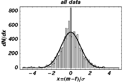
Figure 2: Histogram of the $(measurement-theory)$ for all data points in the CTEQ5m fit.

3 Uncertainties on PDF parameters: The Error Matrix

We now describe results from an investigation of the behavior of the $\chi^{2}_{\rm global}$ function at its minimum, using the standard error matrix approach [21]. This allows us to determine which combinations of parameters are contributing the most to the uncertainty.

At the minimum of $\chi^{2}_{\rm global}$, the first derivatives with respect to the $\{a_{i}\}$ are zero; so near the minimum, $\chi^{2}_{\rm global}$ can be approximated by

$$\chi_{\rm global}^{2}=\chi^{2}_{0}+\frac{1}{2}\sum_{i,j}F_{ij}y_{i}y_{j}$$ (2)

where $y_{i}=a_{i}-a_{0i}$ is the displacement from the minimum, and $F_{ij}$ is the Hessian, the matrix of second derivatives. It is natural to define a new set of coordinates using the complete orthonormal set of eigenvectors of the symmetric matrix $F_{ij}$ as basis vectors. These vectors can be ordered by their eigenvalues $e_{i}$. Each eigenvalue is a quantitative measure of the uncertainties in the shape parameters $\{a_{i}\}$ for displacements in parameter space in the direction of the corresponding eigenvector. The quantity $\ell_{i}\equiv 1/\sqrt{e_{i}}$ is the distance in the 18 dimensional parameter space, in the direction of eigenvector $i$, that makes a unit increase in $\chi^{2}_{\rm global}$. If the only measurement uncertainty were uncorrelated gaussian uncertainties, then $\ell_{i}$ would be one standard deviation from the best fit in the direction of the eigenvector. The inverse of the Hessian is the error matrix.

Because the real uncertainties, for the wide variety of experiments included, are far more complicated than assumed in the ideal situation, the quantitative measure of a given increase in $\chi^{2}_{global}$ carries

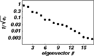
Figure 3: Plot of the eigenvalues of the Hessian. The vertical axis is $\ell_{i}=1/\sqrt{e_{i}}$.

little true statistical meaning. However, qualitatively, the Hessian gives an analytic picture of $\chi^{2}_{\rm global}$ near its minimum in $\{a_{i}\}$ space, and hence allows us to identify the particular degrees of freedom that need further experimental input in future global analyses.

From calculations of the Hessian we find that the eigenvalues vary over a wide range. Figure 3 shows a graph of the eigenvalues of $F_{ij}$, on a logarithmic scale. The vertical axis is $\ell_{i}=1/\sqrt{e_{i}}$, the distance of a “standard deviation” along the $i^{\rm th}$ eigenvector. These distances range over 3 orders of magnitude.Large eigenvalues of $F_{ij}$ correspond to “steep directions” of $\chi^{2}_{\rm global}$. The corresponding eigenvectors are combinations of shape parameters that are well determined by current data. For example, parameters that govern the valence $u$ and $d$ quarks at moderate $x$ are sharply constrained by DIS data. Small eigenvalues of $F_{ij}$ correspond to “flat directions” of $\chi^{2}_{\rm global}$. In the directions of these eigenvectors, $\chi^{2}_{\rm global}$ changes little over large distances in $\{a_{i}\}$ space. For example, parameters that govern the large-$x$ behavior of the gluon distribution, or differences between sea quarks, properties of the nucleon that are not accurately determined by current data, contribute to the flat directions. The existence of flat directions is inevitable in global fitting, because as the data improve it only makes sense to maintain enough flexibility for $f_{a}(x,Q_{0})$ to fit the available experimental constraints.

Because the eigenvalues of the Hessian have a large range of values, efficient calculation of $F_{ij}$ requires an adaptive algorithm. In principle $F_{ij}$ is the matrix of second derivatives at the minimum of $\chi^{2}_{\rm global}$, which could be calculated from very small finite differences. In practice, small computational errors in the evaluation of $\chi^{2}_{\rm global}$ preclude the use of a very small step size. Coarse grained finite differences yield a more accurate calculation of the second derivatives. But because the variation of $\chi^{2}_{\rm global}$ varies markedly in different directions, it is important to use a grid in $\{a_{i}\}$ space with small steps in steep directions and large steps in flat directions. This grid is generated by an iterative procedure, in which $F_{ij}$ converges to a good estimate of the second derivatives.

From calculations of $F_{ij}$ we find that the minimum of $\chi_{\rm global}^{2}$ is fairly quadratic over large distances in the parameter space. Figures 4 and 5

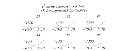
Figure 4: Value of $\chi^{2}$ along the six eigenvectors with the largest eigenvalues.

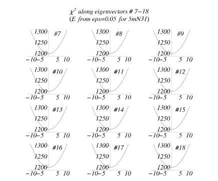
Figure 5: Value of $\chi^{2}$ along the 12 eigenvectors with the smallest eigenvalues.

show the behavior of $\chi^{2}_{\rm global}$ near the minimum along each of the 18 eigenvectors. $\chi^{2}_{\rm global}$ is plotted on the vertical axis, and the variable on the horizontal axis is the distance in $\{a_{i}\}$ space in the direction of the eigenvector, in units of $\ell_{i}=1/\sqrt{e_{i}}$. There is some nonlinearity, but it is small enough that the Hessian can be used as an analytic model of the functional dependence of $\chi^{2}_{\rm global}$ on the shape parameters.

In a future paper we will provide details on the uncertainties of the original shape parameters $\{a_{i}\}$. But it should be remembered that these parameters specify the PDFs at the low $Q$ scale, and applications of PDFs to Tevatron experiments use PDFs at a high $Q$ scale. The evolution equations determine $f(x,Q)$ from $f(x,Q_{0})$, so the functional form at $Q$ depends on the $\{a_{i}\}$ in a complicated way.

4 Uncertainty on $\sigma_{W}$: the Lagrange Multiplier Method

In this Section, we determine the variation of $\chi^{2}_{\rm global}$ as a function of a single measurable quantity. We use the production cross section for $W$ bosons ($\sigma_{W}$) as an archetype example. The same method can be applied to any other physical observable of interest, for instance the Higgs production cross section, or to certain measured differential distributions. The aim is to quantify the uncertainty on that physical observable due to uncertainties of the PDFs integrated over the entire PDF parameter space.

Again, we use the standard CTEQ5 analysis tools and results [5] as the starting point. The “best fit” is the CTEQ5M1 set. A natural way to find the limits of a physical quantity $X$, such as $\sigma_{W}$ at $\sqrt{s}=1.8$ TeV, is to take $X$ as one of the search parameters in the global fit and study the dependence of $\chi^{2}_{\rm global}$ for the 15 base experimental data sets on $X$.

Conceptually, we can think of the function $\chi^{2}_{\rm global}$ that is minimized in the fit as a function of $a_{1},\dots,a_{17},X$ instead of $a_{1},\dots,a_{18}$. This idea could be implemented directly in principle, but a more convenient way to do the same thing in practice is through Lagrange’s method of undetermined multipliers. One minimizes, with respect to the $\{a_{i}\}$, the quantity

$$F(\lambda)=\chi_{\rm global}^{2}+\lambda X(a_{1},\dots,a_{18})$$ (3)

for a fixed value of $\lambda$, the Lagrange multiplier. By minimizing $F(\lambda)$ for many values of $\lambda$, we map out $\chi^{2}_{\rm global}$ as a function of $X$. The minimum of $F$ for a given value of $\lambda$ is the best fit to the data for the corresponding value of $X$, i.e., evaluated at the minimum.

Figure 6 shows $\chi^{2}_{\rm global}$ for the 15 base experimental data sets as a function of $\sigma_{W}$ at the Tevatron. The horizontal axis is $\sigma_{W}$ times the branching ratio for $W\rightarrow$ leptons, in nb. The CTEQ5m prediction is $\sigma_{W}\cdot{BR}_{\rm lep}=2.374$ nb.

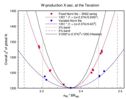
Figure 6: $\chi^{2}$ of the base experimental data sets versus $\sigma_{W}\cdot{BR}_{\rm lep}$, the $W$ production cross-section at the Tevatron times lepton branching ratio, in nb.

The vertical dashed lines are $\pm{3}$% and $\pm{5}$% deviations from the CTEQ5m prediction.

The two parabolas associated with points in Fig. 6 correspond to different treatments of the normalization factor $N_{n}$ in Eq. 1. The dots ($\bullet$) are variable norm fits, in which $N_{n}$ is allowed to float, taking into account the experimental normalization uncertainties, and $F(\lambda)$ is minimized with respect to $N_{n}$. The justification for this procedure is that overall normalization is a common systematic uncertainty. The boxes ($\Box$) are fixed norm fits, in which all $N_{n}$ are held fixed at their values for the global minimum (CTEQ5m). These two procedures represent extremes in the treatment of normalization uncertainty. The parabolas associated with $\bullet$’s and $\Box$’s are just least-square fits to the points.

The other curve in Fig. 6 was calculated using the Hessian method. The Hessian $F_{ij}$ is the matrix of second derivatives of $\chi^{2}_{\rm global}$ with respect to the shape parameters $\{a_{i}\}$. The derivatives (first and second) of $\sigma_{W}$ may also be calculated by finite differences. Using the resultant quadratic approximations for $\chi_{\rm global}^{2}(a)$ and $\sigma_{W}(a)$, one may minimize $\chi^{2}_{\rm global}$ with $\sigma_{W}$ fixed. Since this calculation keeps the normalization factors constant, it should be compared with the fixed norm fits from the Lagrange multiplier method. The fact that the Hessian and Lagrange multiplier methods yield similar results lends support to both approaches; the small difference between them indicates that the quadratic functional approximations for $\chi^{2}_{\rm global}$ and $\sigma_{W}$ are only approximations.

For the quantitative analysis of uncertainties, the important question is: How large an increase in $\chi^{2}_{\rm global}$ should be taken to define the likely range of uncertainty in $X$? There is an elementary statistical theorem that states that $\Delta\chi^{2}=1$ in a constrained fit corresponds to 1 standard deviation of the constrained quantity $X$. However, the theorem relies on the assumption that the uncertainties are gaussian, uncorrelated, and correctly estimated in magnitude. Because these conditions do not hold for the full data set (of $\sim$ 1300 points from 15 different experiments), this theorem cannot be naively applied quantitatively. Indeed, it can be shown that, if the measurement uncertainties are correlated, and the correlation is not properly taken into account in the definition of $\chi_{\rm global}^{2}$, then a standard deviation may vary over the entire range from $\Delta\chi^{2}=1$ to $\Delta\chi^{2}=N$ (the total number of data points – $\sim$ 1300 in our case).

5 Statistical Analysis with Systematic Uncertainties

Fig. 6 shows how the fitting function $\chi_{\rm global}^{2}$ increases from its minimum value, at the best global fit, as the cross-section $\sigma_{W}$ for $W$ production is forced away from the prediction of the global fit. The next step in our analysis of PDF uncertainty is to use that information, or some other analysis, to estimate the uncertainty in $\sigma_{W}$. In ideal circumstances we could say that a certain increase of $\chi_{\rm global}^{2}$ from the minimum value, call it $\Delta\chi^{2}$, would correspond to a standard deviation of the global measurement uncertainty. Then a horizontal line on Fig. 6 at $\chi^{2}_{\rm min}+\Delta\chi^{2}$ would indicate the probable range of $\sigma_{W}$, by the intersection with the parabola of $\chi_{\rm global}^{2}$ versus $\sigma_{W}$.

However, such a simple estimate of the uncertainty of $\sigma_{W}$ is not possible, because the fitting function $\chi^{2}_{\rm global}$ does not include the correlations between systematic uncertainties. The uncertainty $\sigma_{ni}^{d}$ in the definition (1) of $\chi^{2}_{\rm global}$ combines in quadrature the statistical and systematic uncertainties for each data point; that is, it treats the systematic uncertainties as uncorrelated. The standard theorems of statistics for Gaussian probability distributions of random uncertainties do not apply to $\chi^{2}_{\rm global}$.

Instead of using $\chi^{2}_{\rm global}$ to estimate confidence levels on $\sigma_{W}$, we believe the best approach is to carry out a thorough statistical analysis, including the correlations of systematic uncertainties, on individual experiments used in the global fit for which detailed information is available. We will describe here such an analysis for the measurements of $F_{2}(x,Q)$ by the H1 experiment [12] at HERA, as a case study. In a future paper, we will present similar calculations for other experiments.

The H1 experiment has provided a detailed table of measurement uncertainties – statistical and systematic – for their measurements of $F_{2}(x,Q)$. [12] The CTEQ program uses 172 data points from H1 (requiring the cut $Q^{2}>5$ GeV²). For each measurement $d_{j}$ (where $j=1\dots 172$) there is a statistical uncertainty $\sigma_{0j}$, an uncorrelated systematic uncertainty $\sigma_{1j}$, and a set of 4 correlated systematic uncertainties $a_{jk}$ where $k=1\dots 4$. (In fact there are 8 correlated uncertainties listed in the H1 table. These correspond to 4 pairs. Each pair consists of one standard deviation in the positive sense, and one standard deviation in the negative sense, of some experimental parameter. For this first analysis, we have approximated each pair of uncertainties by a single, symmetric combination, equal in magnitude to the average magnitude of the pair.)

To judge the uncertainty of $\sigma_{W}$, as constrained by the H1 data, we will compare the H1 data to the global fits in Fig. 6. The comparison is based on the true, statistical $\chi^{2}$, including the correlated uncertainties, which is given by

$$\chi^{2}=\sum_{j}\frac{\left(d_{j}-t_{j}\right)^{2}}{\sigma_{j}^{2}}-\sum_{kk^{\prime}}B_{k}\left(A^{-1}\right)_{kk^{\prime}}B_{k^{\prime}}.$$ (4)

The index $j$ labels the data points and runs from 1 to 172. The indices $k$ and $k^{\prime}$ label the source of systematic uncertainty and run from 1 to 4. The combined uncorrelated uncertainty $\sigma_{j}$ is $\sqrt{\sigma_{0j}^{2}+\sigma_{1j}^{2}}$. The second term in (4) comes from the correlated uncertainties. $B_{k}$ is the vector

$$B_{k}=\sum_{j}\frac{\left(d_{j}-t_{j}\right)a_{jk}}{\sigma_{j}^{2}},$$ (5)

and $A_{kk^{\prime}}$ is the matrix

$$A_{kk^{\prime}}=\delta_{kk^{\prime}}+\sum_{j}\frac{a_{jk}a_{jk^{\prime}}}{\sigma_{j}^{2}}.$$ (6)

Assuming the published uncertainties $\sigma_{0j}$, $\sigma_{1j}$ and $a_{jk}$ accurately reflect the measurement fluctuations, $\chi^{2}$ would obey a chi-square distribution if the measurements were repeated many times. Therefore the chi-square distribution with 172 degrees of freedom provides a basis for calculating confidence levels for the global fits in Fig. 6.

Lagrange	$\sigma_{W}\cdot{B}$	$\chi^{2}/172$	probability
multiplier	in nb
3000	2.294	1.0847	0.212
2000	2.321	1.0048	0.468
1000	2.356	0.9676	0.605
0	2.374	0.9805	0.558
-1000	2.407	1.0416	0.339
-2000	2.431	1.0949	0.187
-3000	2.450	1.1463	0.092

Table 2: Comparison of H1 data to the PDF fits with constrained values of $\sigma_{W}$.

Table 2 shows $\chi^{2}$ for the H1 data compared to seven of the PDF fits in Fig. 6. The center row of the Table is the global best fit – CTEQ5m. The other rows are fits obtained by the Lagrange multiplier method for different values of the Lagrange multiplier. The best fit to the H1 data, i.e., the smallest $\chi^{2}$, is not CTEQ5m (the best global fit) but rather the fit with Lagrange multiplier 1000 for which $\sigma_{W}$ is 0.8% smaller than the prediction of CTEQ5m. Forcing the $W$ cross section values away from the prediction of CTEQ5m causes an increase in $\chi^{2}$ for the DIS data. At $\sqrt{s}=1.8$ TeV, $W$ production is mainly from $q\bar{q}\rightarrow W^{+}W^{-}$ with moderate values of $x$ for $q$ and $\bar{q}$, i.e., values in the range of DIS experiments. Forcing $\sigma_{W}$ higher (or lower) requires a higher (or lower) valence quark density in the proton, in conflict with the DIS data, so $\chi^{2}$ increases.

The final column in Table 2, labeled “probability”, is computed from the chi-square distribution with 172 degrees of freedom. This quantity is the probability for $\chi^{2}$ to be greater than the value calculated from the existing data, if the H1 measurements were to be repeated. So, for example, the fit with Lagrange multiplier $-3000$, which corresponds to $\sigma_{W}$ being 3.2% larger than the CTEQ5m prediction, has probability 0.092. In other words, if the H1 measurements could be repeated many times, in only 9.2% of trials would $\chi^{2}$ be greater than or equal to the value that has been obtained with the existing data. This probability represents a confidence level for the value of $\sigma_{W}$ that was forced on the PDF by setting the Lagrange multiplier equal to -3000. At the 9.2% confidence level we can say that $\sigma_{W}\cdot{BR}_{\rm lep}$ is less than 2.450 nb, based on the H1 data. Similarly, at the 21.2% confidence level we can say that $\sigma_{W}\cdot{BR}_{\rm lep}$ is greater than 2.294 nb.

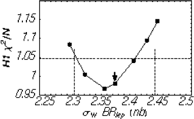
Figure 7: $\chi^{2}/N$ of the H1 data, including error correlations, compared to PDFs obtained by the Lagrange multiplier method for constrained values of $\sigma_{W}$.

Fig. 7 is a graph of $\chi^{2}/N$ for the H1 data compared to the PDF fits in Table 2. This figure may be compared to Fig. 6. The CTEQ5 prediction of the $W$ production cross-section is shown as an arrow, and the vertical dashed lines are $\pm{3}$% away from the CTEQ5m prediction. The horizontal dashed line is the 68% confidence level on $\chi^{2}/N$ for $N=172$ degrees of freedom. The comparison with H1 data alone indicates that the uncertainty on $\sigma_{W}$ is $\sim 3$%.

There is much more to say about $\chi^{2}$ and confidence levels. In a future paper we will discuss statistical calculations for other experiments in the global data set. The H1 experiment is a good case, because for H1 we have detailed information about the correlated uncertainties. But it may be somewhat fortuitous that the $\chi^{2}$ per data point for CTEQ5m is so close to 1 for the H1 data set. In cases where $\chi^{2}/N$ is not close to 1, which can easily happen if the estimated systematic uncertainties are not textbook-like, we must supply further arguments about confidence levels. For experiments with many data points, like 172 for H1, the chi-square distribution is very narrow, so a small inaccuracy in the estimate of $\sigma_{j}$ may translate to a large uncertainty in the calculation of confidence levels based on the absolute value of $\chi^{2}$. Because the estimation of experimental uncertainties introduces some uncertainty in the value of $\chi^{2}$, it is not really the absolute value of $\chi^{2}$ that is important, but rather the relative value compared to the value at the global minimum. Therefore, we might study ratios of $\chi^{2}$’s to interpret the variation of $\chi^{2}$ with $\sigma_{W}$.

6 Conclusions

It has been widely recognized by the HEP community, and it has been emphasized at this workshop, that PDF phenomenology must progress from the past practice of periodic updating of representative PDF sets to a systematic effort to map out the uncertainties, both on the PDFs themselves and on physical observables derived from them. For the analysis of PDF uncertainties, we have only addressed the issues related to the treatment of experimental uncertainties. Equally important for the ultimate goal, one must come to grips with uncertainties associated with theoretical approximations and phenomenological parametrizations. Both of these sources of uncertainties induce highly correlated uncertainties, and they can be numerically more important than experimental uncertainties in some cases. Only a balanced approach is likely to produce truly useful results. Thus, great deal of work lies ahead.

This report described first results from two methods for quantifying the uncertainty of parton distribution functions associated with experimental uncertainties. The specific work is carried out as extensions of the CTEQ5 global analysis. The same methods can be applied using other parton distributions as the starting point, or using a different parametrization of the non-perturbative PDFs. We have indeed tried a variety of such alternatives. The results are all similar to those presented above. The robustness of these results lends confidence to the general conclusions.

The Hessian, or error matrix method reveals the uncertainties of the shape parameters used in the functional parametrization. The behavior of $\chi^{2}_{\rm global}$ in the neighborhood of the minimum is well described by the Hessian if the minimum is quadratic.

The Lagrange multiplier method produces constrained fits, i.e., the best fits to the global data set for specified values of some observable. The increase of $\chi^{2}_{\rm global}$, as the observable is forced away from the predicted value, indicates how well the current data on PDFs determines the observable.

The constrained fits generated by the Lagrange multiplier method may be compared to data from individual experiments, taking into account the uncertainties in the data, to estimate confidence levels for the constrained variable. For example, we estimate that the uncertainty of $\sigma_{W}$ attributable to PDFs is $\pm{3}$%.

Further work is needed to apply these methods to other measurements, such as the $W$ mass or the forward-backward asymmetry of $W$ production in $p\bar{p}$ collisions. Such work will be important in the era of high precision experiments.

PARTON DISTRIBUTION FUNCTION UNCERTAINTIES

Walter T. Giele^a, Stephane A. Keller^b and David A. Kosower^c.

a) Fermi National Accelerator Laboratory, Batavia, IL 60510; b) Theory Division, CERN, CH 1211 Geneva 23, Switzerland; c) CEA–Saclay, F–91191 Gif-sur-Yvette cedex, France.

Abstract

We review the status of our effort to extract parton distribution functions from data with a quantitative estimate of the uncertainties.

1 Introduction

The goal of our work is to extract parton distribution functions (PDF) from data with a quantitative estimation of the uncertainties. There are some qualitative tools that exist to estimate the uncertainties, see e.g. Ref. [1]. These tools are clearly not adequate when the PDF uncertainties become important. One crucial example of a measurement that will need a quantitative assessment of the PDF uncertainty is the planned high precision measurement of the mass of the $W$-vector boson at the Tevatron. Clearly, quantitative tools along the line of S. Alekhin’s pionner work [2] are needed.

The method we have developed in Ref. [3] is flexible and can accommodate non-Gaussian distributions for the uncertainties associated with the data and the fitted parameters as well as all their correlations. New data can be added in the fit without having to redo the whole fit. Experimenters can therefore include their own data into the fit during the analysis phase, as long as correlation with older data can be neglected. Within this method it is trivial to propagate the PDF uncertainties to new observables, there is for example no need to calculate the derivative of the observable with respect to the different PDF parameters. The method also provides tools to assess the goodness of the fit and the compatibility of new data with current fit. The computer code has to be fast as there is a large number of choices in the inputs that need to be tested.

It is clear that some of the uncertainties are difficult to quantify and It might not be possible to quantify all of them. All the plots presented here are for illustration of the method only, our results are preliminary. At the moment we are not including all the sources of uncertainties and our results should therefore be considered as lower limits on the PDF uncertainties. Note that all the techniques we use can be found in books and papers on statistics [4] and/or in Numerical Recipes [5].

2 Outline of the Method

We only give a brief overview of the method in this section. More details are available in Ref.[3]. Our method follows the Bayesian methodology . Once a set of core experiments is selected, a large number of uniformly distributed sets of parameters $\lambda\equiv\lambda_{1},\lambda_{2},\ldots,\lambda_{N_{par}}$ (each set corresponds to one PDF) can be generated and the probability density of the set $P(\lambda)$ calculated from the likelihood (the probability) that the predictions based on $\lambda$ describe the data, see Ref. [4] and next section.

Knowing $P(\lambda)$, then for any observable $x$ (or any quantity that depends on $\lambda$) the probability density, $P(x)$ can be evaluated, and using a Monte Carlo integration, the average value and the standard deviation of $x$ can be calculated with the standard expressions:

$$\mu_{x} = \int\left(\prod_{i=1}^{N_{par}}d\lambda_{i}\right)\,x(\lambda)P(\lambda)$$

$$\sigma_{x}^{2} = \int\left(\prod_{i=1}^{N_{par}}d\lambda_{i}\right)\,(x(\lambda)-\mu_{x})^{2}P(\lambda).$$ (7)

If $P(x)$ is Gaussian distributed, then the standard deviation is a sufficient measure of the PDF uncertainties. If $P(x)$ is not Gaussian distributed, then one should refer to the distribution itself and not try to “summarize” it by a single number, all the information is in the distribution itself. The uncertainties due to the Monte Carlo can also be calculated with standard technique.

The above is correct but computationally inefficient, instead we use a Metropolis algorithm, see Ref. [5], to generate $N_{pdf}$ unit-weighted PDFs distributed according to $P(\lambda)$. With this set of PDFs, the expressions in Eq. 7 become:

$$\mu_{x} \approx \frac{1}{N_{pdf}}\sum_{j=1}^{N_{pdf}}x\left(\lambda_{j}\right)$$

$$\sigma_{x}^{2} \approx \frac{1}{N_{pdf}}\sum_{j=1}^{N_{pdf}}\left(x\left(\lambda_{j}\right)-\mu_{x}\right)^{2}\ .$$ (8)

This is equivalent to importance sampling in Monte Carlo integration techniques. It is very efficient because the number of PDFs needed to reach a given level of accuracy in the evaluation of the integrals is much smaller than when using a set of PDFs uniformly distributed. Given the unit-weighted set of PDFs, a new experiment can be added to the fit by assigning a weight (a new probability) to each of the PDFs, using Bayes’ theorem. The above summations become weighted. There is no need to redo the whole fit if there is no correlation between the old and new data. If we know how to calculate $P(\lambda)$ properly, the only uncertainty in the method comes from the Monte-Carlo integrations.

3 Calculation of $P(\lambda)$

Given a set of experimental points $\{x^{e}\}=x^{e}_{1},x^{e}_{2},\ldots,x^{e}_{N_{obs}}$ the probability of a set of PDF is in fact the conditional probability of $\{\lambda\}$ given that $\{x^{e}\}$ has been measured, this conditional probability can be calculated using Bayes theorem:

$$P(\lambda)=P(\lambda|x^{e})=\frac{P(x^{e}|\lambda)}{P(x^{e})}P_{init}(\lambda),$$ (9)

where, as already mentioned, the prior distribution of the parameters, $P_{init}(\lambda)$, has been assumed to be uniform. A prior sensitivity should be performed. ${P(x^{e}|\lambda)}$ is the likelihood, the probability to observe the data given that the theory is fixed by the set of $\{\lambda\}$ . ${P(x^{e})}$ is the probability density of the data (integrated over the PDFs) and act as a normalization coefficient in Eq. 9.

If all the uncertainties are Gaussian distributed, then it is well known that:

$$P({x^{e}}|\lambda)\approx e^{-\frac{\chi^{2}(\lambda)}{2}},$$ (10)

where $\chi^{2}$ is the usual chi-square:

$$\chi^{2}(\lambda)=\sum_{k,l}^{N_{obs}}\left(x^{e}_{k}-x_{k}^{t}(\lambda)\right)M^{tot}_{kl}\left(x^{e}_{l}-x_{l}^{t}(\lambda)\right)\ ,$$ (11)

$x_{k}^{t}(\lambda)$ are the theory prediction for the experimental observables calculated with the parameters $\{\lambda\}$ . The matrix $M^{tot}$ is the inverse of the total covariance matrix.

When the uncertainties are not Gaussian distributed, the result is not as well known. We first present two simple examples to illustrate how the likelihood should be calculate and then give a generalization.

3.1 The simplest example

We first consider the simplest example to setup the notation, one experimental point with a statistical uncertainty:

$$x^{t}(\lambda)=x^{e}+u\Delta,$$ (12)

where $u$ is a random variable that has it own distribution, f(u) (assumed to be Gaussian in this case). By convention, we take the average of $u$ equal to 0 and its standard deviation equal to 1. $\Delta$ gives the size of the statistical uncertainty. For each experimental measurement there is a different value of $u$ and $x^{e}$. The probability to find $x^{e}$ in an element of length $dx^{e}$ given that the theory is fixed by $\{\lambda\}$ is equal to the probability to find $u$ in a corresponding element of length $du$:

$$P({x^{e}}|\lambda)dx^{e}=f(u)du.$$ (13)

The variable $u$ and the Jacobian for the change of variable from $u$ to $x^{e}$ can be extracted from Eq. 12:

$$u=\frac{x^{t}(\lambda)-x^{e}}{\Delta};\left|\frac{du}{dx^{e}}\right|=\frac{1}{\Delta}$$ (14)

such that:

$$P({x^{e}}|\lambda) = \frac{f(\frac{x^{t}(\lambda)-x^{e}}{\Delta})}{\Delta}$$ (15)

$$= \frac{1}{\sqrt{2\pi}\Delta}e^{{-\frac{(x^{t}-x^{e})^{2}}{2\Delta^{2}}}}.$$

This is the expected result.

3.2 A simple example

We now consider the case of one experimental point with a statistical and a systematic uncertainty:

$$x^{t}(\lambda)=x^{e}+u_{1}\Delta_{1}+u_{2}\Delta_{2}$$ (16)

$\Delta_{1}$ and $\Delta_{2}$ give the size of the uncertainties. $u_{1}$ and $u_{2}$ have their own distribution $f^{1}(u_{1})$ and $f^{2}(u_{2})$ and we use the same convention for their average and standard deviation as for $u$ in the first example. This time for each experimental measurement, there is an infinite number of sets of $u_{1},u_{2}$ that correspond to it, because there is only one equation that relate $x^{t}$, $x^{e}$ and $u_{1}$ and $u_{2}$. The probability to find $x^{e}$ in an element of length $dx^{e}$ given that the theory is fixed by $\{\lambda\}$ is here equal to the probability to find $u_{1}$ and $u_{2}$ in a corresponding element of area $du_{1}\,du_{2}$, with an integration over one of the two variables:

$$P(x^{e}|\lambda)dx^{e}=du^{1}\int du_{2}f^{1}(u_{1})f^{2}(u_{2}).$$ (17)

We choose to integrate over $u_{2}$. $u_{1}$ and the Jacobian for the change of variable from $u_{1}$ to $x^{e}$ are given by Eq. 16:

$$u_{1}=\frac{x^{t}-x^{e}-u_{2}\Delta_{2}}{\Delta_{1}};\left|\frac{du_{1}}{dx^{e}}\right|=\frac{1}{\Delta_{1}}$$ (18)

such that:

$$P(x^{e}|\lambda)=\int du_{2}f^{2}(u_{2})\frac{f^{1}(\frac{x^{t}-x^{e}-u_{2}\Delta_{2}}{\Delta_{1}})}{\Delta_{1}}$$ (19)

If both $f^{1}(u_{1})$ and $f^{2}(u_{2})$ are Gaussian distribution then we recover the expected result, as in Eq 10. Note that this expected result is recovered if the uncertainties are Gaussian distributed and the relationship between the theory, the data and the uncertainties are given by Eq. 16. If that relationship is more complex there is no guarantee to recover Eq. 10. In the general case, the integral in Eq. 19 has to be done numerically.

3.3 Generalization:

We are now ready to give a generalization of the calculation of the likelihood. We are considering $N_{obs}$ observables, and $N_{unc}$ uncertainties (statistical and systematic) parametrised by $N_{unc}$ random variables $\{u\}=u_{1},u_{2},\ldots,u_{N_{unc}}$ with their own distributions, $f^{i}(u_{i})$.

There are $N_{obs}$ relations between $\{x^{t}\}$, $\{x^{e}\}$ and $\{u\}$, one for each observable:

$$F_{i}(x_{i}^{e},\{x^{t}(\lambda)\},\{u\})=0.$$ (20)

This gives $N_{unc}-N_{obs}$ independent $u_{i}$ that we choose by convenience to be the $u_{i}^{\prime}s$ corresponding to the systematic uncertainties. Without loosing generality we assume that there is one statistical uncertainty for each observable, and we organize the corresponding $u_{i}$ with the same index as $x^{e}_{i}$, such that the last $N_{sys}$($=N_{unc}-N_{obs}$) $u_{i}$ are the random variables for the systematic uncertainties. For each set of measured $\{x^{e}\}$ there is an infinite number of $\{u\}$ sets that correspond to it.

The probability to find $\{x^{e}\}$ in an element of volume $\prod_{i=1}^{N_{obs}}dx^{e}_{i}$ given that the theory is fixed by $\{\lambda\}$ is equal to the probability to find the $\{u\}$ in a corresponding element of volume $\prod_{i=1}^{N_{unc}}dx^{u}$ , with an integration over the independent $u_{i}$ :

$$P(\{x^{e}\}|\lambda)\prod_{i=1}^{N_{obs}}dx^{e}_{i} = (\prod_{k=1}^{N_{obs}}du_{k})\int(\prod_{i=N_{obs}+1}^{N_{unc}}du_{i})$$ (21)

$$*\ \ \prod_{j=1}^{N_{unc}}f^{j}(u_{j})$$

The values of the $\{u_{i},i=1,N_{obs}\}$ (corresponding to the statistical uncertainties) and the Jacobian, $J(u\rightarrow x^{e})$, for the change of variable from those $u_{i}$ to the $x^{e}_{i}$ can be extracted from the $N_{obs}$ relations in Eq. 20. The likelihood is then given by:

$$P(\{x^{e}\}|\lambda)=\int(\prod_{i=N_{obs}+1}^{N_{unc}}du_{i})\ \ \prod_{j=1}^{N_{unc}}f^{j}(u_{j})J(u\rightarrow x^{e})$$ (22)

Often, the $F_{i}$ relationship in Eq 20 have a simple dependence on $\{x^{e}\}$ and the $u^{\prime}s$ corresponding to the statistical uncertainties:

$$F_{i}(x_{i}^{e},\{x^{t}(\lambda)\},\{u\})=x_{i}^{e}+u_{i}\Delta_{i}+\cdots,$$ (23)

where the $\Delta_{i}$ are the size of the statistical uncertainties. In that case, the Jacobian is simply given by:

$$J(u\rightarrow x^{e})=\prod_{i=1}^{N_{obs}}\frac{1}{\Delta_{i}}$$ (24)

In most cases, the likelihood will not be analytically calculable, and has to be calculated numerically again with Monte Carlo technique.

In order to be able to calculate the likelihood we therefore need:

• the relations between $\{x^{t}\}$, $\{x^{e}\}$ and $\{u\}$ as in Eq. 20.

• the probability distribution of the random variable associated with the uncertainties: $f^{i}(u_{i})$.

Unfortunately most of the time that information is not reported by the experimenters, and/or is not available and certainly difficult to extract from papers. It is only in the case that all the uncertainties are Gaussian distributed  that it is sufficient to report the size of the uncertainties and their correlation . This is a very important issue, simply put, experiments should always provide a way to calculate the likelihood, $P(\{x^{e}\}|\lambda)$. This last fact was also the unanimous conclusion of a recent workshop on confidence limits held at CERN [7]. This is particularly crucial when combining different experiments together: the pull of each experiment will depend on it and, as a result, so will the central values of the deduced PDFs.

3.4 The central limit theorem

Assuming that the uncertainties are Gaussian distributed when they are not can lead to some serious problems. For example, minimizing the $\chi^{2}$ constructed assuming Gaussian distribution will not even maximize the likelihood. Indeed in the general case, the usually defined $\chi^{2}$ will not appear in the likelihood.

It is often assumed that the central limit theorem can be used to justify the assumption of Gaussian distribution for the uncertainties. It is therefore useful to revisit this theorem. $Y$ is a linear combination of $n$ independent $X_{i}$:

$$Y=\sum_{i}c_{i}X_{i}$$ (25)

$$\sigma_{Y}^{2}=\sum_{i}c_{i}^{2}\sigma_{X_{i}}^{2}$$

where the $c_{i}$ are constants and the $\sigma$ are the standard deviations. The theorem states that in the limit of large $n$ the distribution of $Y$ will be approximately Gaussian if $\sigma_{Y}^{2}$ is much larger than any component $c_{i}^{2}\sigma_{X_{i}}^{2}$ from a non-Gaussian distributed $X_{i}$. For some examples of how large $n$ has to be, see Ref. [4].

Here is one way the theorem could be used: If the $F_{i}$ relations are given by:

$$x^{t}_{i}(\lambda)=x^{e}_{i}+\sum_{k=1}^{N_{unc}}u_{k}\Delta_{ik}$$

and if there is a large number of uncertainties, the $u_{k}$ are independent and none of the $\Delta_{ik}$ for a non-Gaussian-like $u_{k}$ dominate then we know that the sum will be approximately Gaussian distributed. One way to express this fact is simply to assume that all the uncertainties are Gaussian distributed. In this case, we recover the usual expression for the likelihood.

A direct consequence is that if there are a few uncertainties that dominate a measurement, then we certainly need to know their distribution. See Ref. [8], for an example of a non-Gaussian dominant uncertainty in a real life experiment.

3.5 Luminosity Uncertainty

We now turn to the calculation of the likelihood when there is a normalization uncertainty, like the Luminosity uncertainty. The $F$ relation of Eq. 20 is given by:

$${\cal L}\lambda=x^{e}+u_{1}\Delta_{1},$$ (26)

where we have assumed that we are measuring the parameter directly, $x^{t}=\lambda$. The Luminosity, ${\cal L}$, has also an uncertainty:

$${\cal L}={\cal L}_{0}+u_{2}\Delta_{2}.$$ (27)

We assume that both $u_{1}$ and $u_{2}$ are Gaussian distributed. Replacing Eq. 27 in Eq. 26, we obtain:

$${\cal L}_{0}\lambda-x^{e}=u_{1}\Delta_{1}-u_{2}\Delta_{2}x^{t}.$$ (28)

This expression shows that ${\cal L}_{0}\lambda-x^{e}$ is the sum of two Gaussian, such that the likelihood is a Gaussian distribution with the standard deviation given by:

$$\sigma^{2}=\Delta_{1}^{2}+(\Delta_{2}x^{t})^{2}.$$ (29)

The systematic uncertainty due to the Luminosity uncertainty is proportional to the theory. Explicitly:

$$P(x^{e}|\lambda)=\frac{1}{\sqrt{2\pi}\sqrt{\Delta_{1}^{2}+(\Delta_{2}\lambda)^{2}}}e^{-\frac{(L_{0}\lambda-x^{e})^{2}}{2(\Delta_{1}^{2}+(\Delta_{2}\lambda)^{2})}}$$ (30)

This result can also be derived from the general expression of the likelihood, after doing the appropriate integral analytically.

A few remarks are in order. In this case, eventhough all the uncertainties are Gaussian distributed, the minimization of the $\chi^{2}$ would not maximize the likelihood because the theory appears in the normalization of the likelihood. Another mistake that leads to problems in this case is to replace $\lambda$ by $x^{e}/{\cal L}_{0}$ in the uncertainty. This mistake leads to a downwards bias. If $x^{e}$ has a downward statistical fluctuation, a smaller systematic uncertainty is assigned to it, such that when it is combined with other measurements, it is given a larger weight than it should.

This example shows clearly that we have to know if the uncertainties are proportional to the theory or to the experimental value. Assuming one when the other is correct can lead to problems. It is clear that many other systematic uncertainties depend on the theory and that should also be taken into account.

4 Sources of uncertainties

There are many sources of uncertainties beside the experimental uncertainties. They either have to be shown to be small enough to be neglected or they need to be included in the PDF uncertainties. For examples: variation of the renormalization and factorization scales; non-perturbative and nuclear binding effects; the choice of functional form of the input PDF at the initial scale; accuracy of the evolution; Monte-Carlo uncertainties; and dependence on theory cut-off.

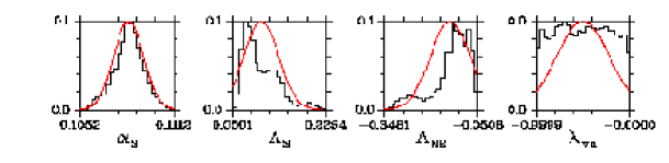
Figure 8: Plot of the distribution (black histograms) of four of the parameters. The first one is $\alpha_{s}$, the strong coupling constant at the mass of the $Z$-boson. The line is a Gaussian distribution with same average and standard deviation as the histogram

5 Current fit

Draconian measures were needed to restart from scratch and re-evaluate each issue. We fixed the renormalization and factorisation scales, avoided data affected by nuclear binding and non-perturbative effects, and use a MRS-style parametrization for the input PDFs. The evolution of the PDFs is done by Mellin transform method, see Ref. [9]. All the quarks are considered massless. We imposed a positivity constraint on F2. A positivity constraint on other “observables” could also be imposed.

At the moment we are using H1 and BCDMS (proton data) measurement of $F_{2}^{p}$ for our core set. In order to be able to use these data we have to assume that all the uncertainties are Gaussian distributed . We then can calculate the $\chi^{2}(\lambda)$ and $P(\lambda)$ ($\approx\exp{-\chi^{2}/2}$) with all the correlations taken into account . We generated 50000 unit-weighted PDFs according to the probability function. For 532 data points, we obtained a minimum $\chi^{2}$ of 530 for 24 parameters. We have plotted in Fig. 8, the probability distribution of some of the parameters. Note that the first parameter is $\alpha_{s}$. The value is smaller than the current world average. However, it is known that the experiments we are using prefer a lower value of this parameter, see Ref. [10], and as already pointed out, our current uncertainties are lower limits. Note that the distribution of the parameter is not Gaussian, indicating that the asymptotic region is not reached yet. In this case, the blind use of the so-called chi-squared fitting method might be misleading.

From this large set of PDFs, it is straightforward to plot, for example, the correlation between different parameters and to propagate the uncertainties to other observables. In Fig. 9,

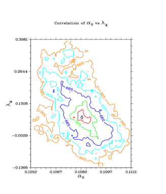
Figure 9: Correlation between two of the parameters: $\alpha_{s}$ and $\lambda_{g}$, see the text for their definition. Constant probability density levels are plotted.

the correlation between $\alpha_{s}$ and $\lambda_{g}$ is presented. $\lambda_{g}$ parametrizes the small Bjorken-$x$ behavior of the gluon distribution function at the initial scale: $xg(x)\sim x^{-\lambda_{g}}$. The lines are constant probability density levels that are characterized by a percentage, $\alpha$, wich is defined such that $1-\alpha$ is the ratio of the probability density corresponding to the level to the maximum probability density.

In Fig. 10, we show the correlation between two

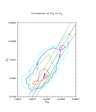
Figure 10: Correlation between the production cross sections for the $W$ and $Z$ vector bosons at the Tevatron, $\sigma_{W}$ and $\sigma_{Z}$ (in nbarns, includes leptonic branching fraction). The solid and dashed lines show the constraint due to the CDF measurement of the cross section ratio.

observables, the production cross sections for the $W$ and $Z$ vector bosons at the Tevatron along with the experimental result from CDF. The constant probability density levels are shown. The agreement between the theory and the data is qualitatively good.

In Fig. 11, we present data-theory for the lepton charge

Figure 11: Data-theory for the lepton charge asymmetry in $W$ decay at the Tevatron.

asymmetry in $W$ decay at the Tevatron. The data are the CDF result [11] and the theory correspond to the average value over the PDF sets for each data point, as defined in Eq. 7. The dashed line are the theory plots corresponding to the one standard deviation over the PDF sets, also defined in Eq. 7. The inner error bars are the statistical and systematic uncertainties added in quadrature. The outer error bar correspond to the experiment and theory uncertainties added in quadrature. The theory uncertainty is the uncertainty associated with the Monte-Carlo integration, the factorization and renormalization scale dependence are small and can be neglected. 5000 PDFs were used to generate this plot. It is well known that the data we have included so far in our fit mainly constraint the sum of the quark parton distribution weighted by the square of the charges. The lepton charge asymmetry is sensitive to the ratio of up-type to down-type quark and is therefore not well constraint. We can add this data set by simply weighting each PDF from our set with the likelihood of the new data. The resulting new range of the theory (calculated with weighted sums) is given by the band of solid curves in Fig 11.

The effect of the inclusion of the lepton charge asymmetry can be seen in Fig. 12, where the correlation between

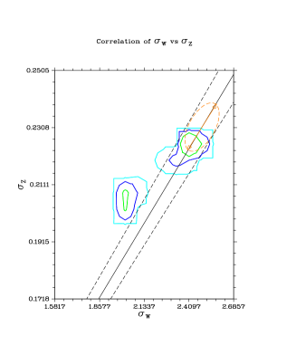
Figure 12: Same as in Fig. 10 for the weighted PDFs.

the $W$ and the $Z$ cross section is shown again but for the weighted PDFs. The agreement with the data is better than before, but the probability density has now two maxima.

It has been argued that for Run II at the Tevatron, the measurement of the number of $W$ and $Z$ produced could be used as a measurement of the Luminosity. That of course requires the knowledge of the cross section with a small enough uncertainties. In Fig. 13, the luminosity probability

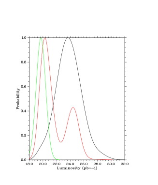
Figure 13: Probability distribution of the luminosity (run1a in $pb^{-1}$) for the unit-weighted (right plot) and weighted (middle plot) PDFs, compared to the value used by CDF (left plot).

distribution is presented for the unit-weighted and weighted PDF sets along with the the luminosity used by CDF. The plot for the weighted set has also two maxima, has in Fig. 12.

5.1 Conclusions

In conclusion, we remind the reader again that all the results should be taken as illustration of the method and that not all the uncertainties have been included in the fitting.

EXPERIMENTAL UNCERTAINTIES AND THEIR DISTRIBUTIONS IN THE INCLUSIVE JET CROSS SECTION.

R. Hirosky
University of Illinois, Chicago, IL 60607

1 Introduction

This workshop has been an important channel of communication between those performing global parton distribution function (pdf) fits and the experimental groups who provide the data at the Tevatron. In the particular case of jets analyses we have initiated a detailed dialog on the sources and distributions of experimental uncertainties. As part of my participation in the workshop, I have used the DØ inclusive jet cross section as an example of a jet measurement with a complex ensemble of uncertainties and have provided descriptions of each component uncertainty. Such dialogs will prove crucial in obtaining the best constraints on allowable pdf models from the data.

2 Uncertainties on the CDF and DØ inclusive jet cross sections

In the first meeting we summarized the jet inclusive cross section measurements from the DØ [1] and CDF [2] experiments. In particular, we illustrated the major corrections applied to the data, namely jet $E_{T}$ scale and $E_{T}$ resolution corrections, as well as the derivation methods for these corrections employed by each experiment. To review these methods see [3]-[4] and references therein.

The uncertainties by component in the CDF and DØ inclusive jet cross sections are shown in Figs.14-15. Each component of the uncertainty reported for the CDF cross section is taken to be completely correlated across jet $E_{T}$, while individual components are independent of one another. The DØ uncertainties (shown here symmetrized) are also independent of one another, however each component may be either fully or partially correlated across jet $E_{T}$. In the case of the energy scale uncertainty the band shown is constructed from eight subcomponents.

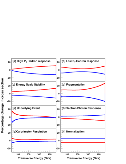
Figure 14: Uncertainties by component in the CDF inclusive jet cross section, $1/(\Delta\eta\Delta E_{T})\int\int d^{2}\sigma/(dE_{T}d\eta)dE_{T}d\eta$, $0.1<|\eta|<0.7$

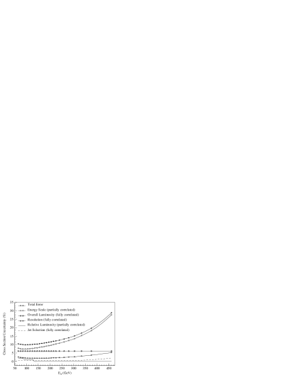
Figure 15: Uncertainties by component in the DØ  inclusive jet cross section, $1/(\Delta\eta\Delta E_{T})\int\int d^{2}\sigma/(dE_{T}d\eta)dE_{T}d\eta$, $|\eta|<0.5$

2.1 Comparisons with theory

The two experiments have used various means to compare their measurements to theoretical predictions. CDF has published a comparison of their cross section to a next-to-leading order (NLO) QCD calculation using a variety of pdf models by means of various normalization-insensitive, shape-dependent statistical measures [2] (Kolmogorov-Smirnov, Cramèr-VonMises, Anderson-Darling). DØ has formulated a covariance matrix using each uncertainty component in the cross section and its $E_{T}$ correlation information and employed a $\chi^{2}$ test to compare to NLO QCD [1]. It is difficult to generalize the various shape statistics to include non-trivial correlations in the systematic uncertainties and although correlations may be easily added to a covariant error matrix $\chi^{2}$ tests can show biases when faced with correlated scale errors. Reference [6] illustrates how correlated scale errors may lead to biases in parameter estimation by noting that systematic errors reported as a fraction of the observed data can be evaluated as artificially small when applied to a point that fluctuates low. This bias may be mitigated by parameterizing the systematic scale errors as percentages of a smooth model of the data or by placing them on the smooth theory directly (see contributions to these proceedings by W. Giele, S. Keller, and D. Kosower).

Other difficulties arise in interpretation of $\chi^{2}$ probabilities when uncertainties show large correlations. The probability that a prediction agrees with the data for a given $\chi^{2}$ is calculated assuming that the $\chi^{2}$ follows the distribution:

$$f(x;n)=\frac{(x)^{(n/2-1)}exp(x/2)}{2^{(n/2)}\Gamma(n/2)}$$ (31)

where $n$ is the number of degrees of freedom of the data set. The probability of getting a worse value of $\chi^{2}$ than the one obtained for the comparison is given by:

$$P(\chi^{2};n)=\int_{\chi^{2}}^{\infty}f(x;n)dx$$ (32)

Hence, to verify the accuracy of the probabilities quoted in the recent DØ cross section papers (inclusive jet cross section [1] and dijet mass spectrum [7]), the $\chi^{2}$ distribution may be compared to Equation 31 with the appropriate number of degrees of freedom. The $\chi^{2}$ distribution for the DØ dijet mass spectrum was tested by developing a Monte Carlo program [8] that generates many trial experiments based an ansatz cross section determined from the best smooth fit to the data (with a total of 15 bins, or 15 degrees of freedom). The first step generated trials based on statistical fluctuations taking the true number of events per bin as given by the ansatz cross section. The trial spectra were then generated for each bin according to Poisson statistics. The $\chi^{2}$ for each of these trials was calculated using the difference between the true and the generated values. Figure 16 (solid curve) shows the $\chi^{2}$ distribution for all of the generated trials. The distribution agrees well with Equation 31 for 15 degrees of freedom. The next step assumes that the uncertainties correlated as in the measurement of the dijet mass cross section. Trial spectra are generated using these uncertainties to generate a $\chi^{2}$ distribution (see the dotted curve in Fig. 16). It is clear that $\chi^{2}$ distribution very similar to the curve predicted by Equation 31. Hence, any probability generated using Equation 32 will be approximately correct. The resulting $\chi^{2}$ distribution was fitted by Equation 31 and the resulting fit is consistent with the distribution if 14.6 degrees of freedom are assumed.

Figure 16: $\chi^{2}$ distribution for random fluctuations around the nominal DØ Dijet Mass cross section. (Solid) Errors are fluctuated as uncorrelated. (Dashed) $E_{T}$ correlations are included.

A similar test using the DØ inclusive jet cross section finds the distributions shown in Fig. 17. The two distributions agree well for $\chi^{2}$ values below approximately 15 and then begin to diverge slowly. The distribution based on the cross section uncertainties includes a larger tail than the $\chi^{2}$ distribution generated with the wholly uncorrelated uncertainties, implying that probabilities based on a $\chi^{2}$ analysis will be slightly underestimated. See also the talks by B. Flaugher in this workshop for additional observations and comments on $\chi^{2}$ analyses.

Figure 17: $\chi^{2}$ distribution for random fluctuations around the nominal DØ inclusive jet cross section. (Solid) errors are fluctuated as uncorrelated. (Dashed) $E_{T}$ correlations are included.

3 Beyond the Normal assumption

Independent of any difficulties due to correlated uncertainties, a $\chi^{2}$ test necessarily relies on the assumption that the uncertainties follow a normal distribution. This may be a reasonable approximation in some cases. Upon close inspection we expect this assumption to be generally false for most rapidly varying observables (i.e. steeply falling cross section measurements). Perhaps, as in the most obvious case, some experimental uncertainties will simply be non-Gaussian in their distribution and furthermore symmetric uncertainties in the abscissa variable will develop into asymmetric uncertainties when propagated through to the measured distribution. The latter case is illustrated as follows. Consider an $E_{T}$-independent jet $E_{T}$ scale error of 2%. What is it’s effect on an inclusive jet cross section versus $E_{T}$? Jets are shifted bin-to-bin by fluctuating their $E_{T}$ values within the 2% range and as a result of the steeply falling cross section, more jets from low $E_{T}$ values are shifted into higher $E_{T}$ bins by one extreme of this scale uncertainty than the in reverse shift for higher $E_{T}$ jets. Figure. 18 shows how a flat 2% $E_{T}$ scale uncertainty alters the measured cross section using a smooth fit to the DØ data as the nominal cross section model. In general the degree of this asymmetry will depend on the steepness of the measured distribution. In order to define a covariance matrix, such errors are typically symmetrized.

Figure 18: Example of a 2% $E_{T}$ scale error propagated through an inclusive jet cross section measurement.

The use of an approximate covariance matrix will also result in a loss of sensitivity when errors are shown to follow distributions with tails smaller than in a normal distribution. As an example we show a correction factor with uncertainties of this type from the DØ jet cross section analysis in Fig. 19. This figure shows the hadronic response correction for jets as a function of jet energy. The correction is derived from an analysis of $\gamma+jet$ data [4]. The bands delimit regions that contain ensembles of deviations from the nominal response within certain confidence limits. It is evident that in this case assuming the uncertainty follows a normal distribution with variance equal to the 68% limits shown will tend of underestimate the sensitivity of the data for excluding certain classes of theories. Figure 20 shows the range of cross section uncertainty due to the response component only as a function of confidence level for several $E_{T}$ values of the DØ cross section.

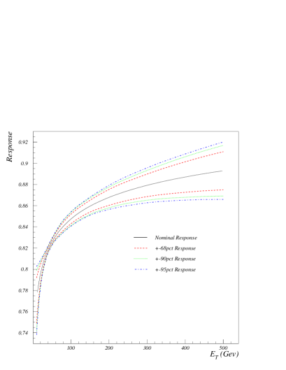
Figure 19: DØ Jet response correction versus Energy. The outer bands show the extreme deviation in response at a given confidence level as a function of jet energy.

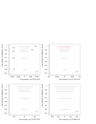
Figure 20: DØ response uncertainty propagated through the inclusive jet cross section measurement at various $E_{T}$ values. The solid bands represent extreme variations at various confidence levels. The dashed bands illustrate the overestimation of these variations by using a Gaussian approximation.

4 Application to pdf constraints

In this workshop W. Giele, S. Keller, and D. Kosower have reported on a method for extracting pdf distributions with quantitative estimates of pdf uncertainties. In effect their method [5] uses a Bayesian approach that integrates sets of pdf parameterizations over properly weighted samples of experimental uncertainties to produce a set of pdf models consistent with the data within a given confidence level. The basic method may be extended to use data with arbitrary error distributions and correlations. For such methods to function reliably the experiments must be able to provide detailed descriptions of their error distributions. Giele et al. make a distinction between ‘errors on the data’ and ‘errors on the theory’ for estimation of the most likely pdf models. In this context we take only uncertainties depending directly on the number of events in a bin as ‘errors on the data’. Other typical sources of uncertainty, luminosity, energy scale, resolution, etc., may be treated as ‘errors on the theory’ in that they are in some sense independent of the statistical precision of the data and represent how an underlying, true, distribution may be distorted by observation in the experiment.

As a result of these dialogs, we have revisited the DØ response uncertainty (our largest uncertainty in the inclusive jet cross section measurement) from Fig. 19 and generated a sampling of the probability density function for distributions in it parameters. This probability density function contains all the relevant information on both the shape of the uncertainty distribution and point-to-point correlations. It is clear that providing such information is a significant enhancement from traditional methods of summarizing experimental uncertainties. Optimum utilization of the data demands a detailed understanding and reporting of its associated uncertainties. Through our fruitful discussions in this workshop, we look forward to setting an example for the reporting of experimental uncertainties and to fully exploiting our cross section data in pdf analyses in the near future.

PARTON DENSITY UNCERTAINTIES AND SUSY PARTICLE PRODUCTION

T. Plehn^a, and M. Krämer^b,

a) Department of Physics, University of Wisconsin, Madison WI 53706, USA; b) Department of Physics and Astronomy, University of Edinburgh, Edinburgh EH9 3JZ, Scotland.

Abstract

Parton densities are important input parameters for SUSY particle cross section predictions at the Tevatron. Accurate theoretical estimates are needed to translate experimental limits, or measured cross sections, into SUSY particle mass bounds or mass determinations. We study the PDF dependence of next-to-leading order cross section predictions, with emphasis on a new set of parton densities [1]. We compare the resulting error to the remaining theoretical uncertainty due to renormalization and factorization scale variation in next-to-leading order SUSY-QCD.

1 Introduction

The search for supersymmetric particles is among the most important endeavors of present and future high energy physics. At the upgraded $p\bar{p}$ collider Tevatron, the searches for squarks and gluinos (and especially the lighter stops and sbottoms), as well as for the weakly interacting charginos and neutralinos, will cover a wide range of the MSSM parameter space [2, 3].

The hadronic cross sections for the production of SUSY particles generally suffer from unknown theoretical errors at the Born level [4]. For strongly interacting particles the dependence on the renormalization and factorization scale has been used as a measure for this uncertainty, leading to numerical ambiguities of the order of 100$\%$. For Drell-Yan type weak production processes the dependence on the factorization scale is mild. However, a comparison of leading and next-to-leading order predictions [5] reveals that the impact of higher-order corrections is much larger than the estimate through scale variation would have suggested. The use of next-to-leading order calculations [5, 6, 7] is thus mandatory to reduce theoretical uncertainties to a level at which one can reliably extract mass limits from the experimental data.

In addition to the scale ambiguity and the impact of perturbative corrections beyond next-to-leading order, hadron collider cross section are subject to uncertainties coming from the parton densities and the associated value of the strong coupling. Previously, the only way to estimate the PDF errors was to compare the best-fit results from various global PDF analyses. Clearly, this is not a reliable measure of the true uncertainty. As a first step towards a more accurate error estimate, the widely used sets CTEQ [8] and MRST [9] now offer different variants of PDF sets, e.g. using different values of the strong coupling constant. In this letter we compare their predictions to the preliminary GKK parton densities [1], which provide a systematic way of propagating the uncertainties in the PDF determination to new observables.

2 Stop Pair Production

For third generation squarks the off-diagonal left-right mass matrix elements do not vanish, but lead to mixing stop (and sbottom) states. The lighter mass eigenstate, denoted as $\tilde{t}_{1}$, is expected to be the lightest strongly interacting supersymmetric particle. Moreover, its pair production cross section, to a very good approximation, only depends on the stop mass, in contrast to the light flavor squark production. Nevertheless, considering the different decay channels complicates the analyses [3, 10]. At the Tevatron the fraction of stops produced in quark-antiquark annihilation and in gluon fusion varies strongly with the stop mass. Close to threshold the valence quark luminosity is dominant, but for lower masses a third of the hadronic cross section can be due to incoming gluons [7].

In Figure 21 we compare the total $\tilde{t}_{1}$-pair production cross sections for three sets of parton densities: only for incoming quarks do the CTEQ4 and MRST99 results lie on top of each other. For gluon fusion the corresponding cross sections differ by $\sim 10\%$. The GKK set centers around a significantly smaller value. This is in part due to the low average value $\langle\alpha_{s}({\rm GKK})\rangle=0.108$, which is expected to increase after including more experimental information in the GKK analysis. But even the normalized cross section $\sigma/\alpha_{s}^{2}$ is still smaller by $35\%$ compared to CTEQ4 and MRST99 because of the entangled fit of the strong coupling constant and the parton densities. However, the width of the Gaussian fit to the GKK results gives an uncertainty of $2\%$ and $8\%$ for the quark-antiquark and gluon fusion channel, similar to the difference between CTEQ4 and MRST99.

For heavier stop particles, Figure 22, the gluon luminosity is strongly suppressed due to the large final state mass, and mainly valence quarks induced processes contribute to the cross section. The Gaussian distribution of the GKK results has a width of $\sim 2\%$. The comparably large difference between CTEQ4 and MRST99 is caused by the small fraction of gluon induced processes, since the gluon flux at large values of $x$ differs for CTEQ4 and MRST99 by approximately $40\%$.

3 Chargino/Neutralino Production

The production of charginos and neutralinos at the Tevatron is particularly interesting in the trilepton $\tilde{\chi}_{2}^{0}\tilde{\chi}_{1}^{\pm}$ and the light chargino $\tilde{\chi}_{1}^{+}\tilde{\chi}_{1}^{-}$ channels [11]. The next-to-leading order corrections to the cross sections [5] reduce the factorization scale dependence, but at the same time introduce a small renormalization scale dependence. A reliable estimate of the theoretical error from the scale ambiguity will thus only be possible beyond next-to-leading order.

The Gaussian distribution of the GKK parton densities for light chargino pairs is shown in Figure 23. For the chosen mSUGRA parameters ($m_{0}=100\;\mbox{Ge$\!$V},A_{0}=300\;\mbox{Ge$\!$V},m_{1/2}=150\;\mbox{Ge$\!$V}$) the width is $\sim 2\%$, as one would expect from the quark-antiquark channel of the stop production. But in contrast to the stop production, where all quark luminosities add up, the chargino/neutralino channels can be extremely sensitive to systematic errors in different parton densities due to destructive interference between $s$ and $t$ channel diagrams. The total trilepton cross section for example will therefore be a particular challenge for a reliable error estimate.

4 Outlook

We have briefly reviewed the status of the theoretical error analysis of SUSY cross sections at the Tevatron. For strongly interacting final state particles, the inclusion of next-to-leading order corrections reduces the renormalization and factorization scale ambiguity to a level $\hbox to0.0pt{\lower 3.5pt\hbox{$\mathchar 0\relax\sim$}\hss}\raise 1.0pt\hbox{$<$}\;10\%$ where the size of the PDF errors becomes phenomenologically relevant. We have compared different recent PDF sets provided by the CTEQ [8] and MRST [9] collaborations to the preliminary GKK parton densities [1]. The large spread in the cross section predictions can mainly be attributed to the low average value of the strong coupling associated with the GKK sets. We expect this spread to be reduced once more data have been included in the GKK analysis and the corresponding average value of the strong coupling becomes closer to the world average. For weak supersymmetric Drell-Yan type processes [5] the scale dependence at NLO cannot serve as a measure for the theoretical error since the renormalization scale dependence is only introduced at NLO. The PDF induced errors for e.g. the case of $\tilde{\chi}_{1}^{+}\tilde{\chi}_{1}^{-}$ production are small; however, interference effects between the different partonic contributions must be taken into account.

The recently available variants of PDF sets provided by CTEQ and MRST and, in particular, the GKK parton densities allow for the first time a systematic exploration of PDF uncertainties for the prediction of SUSY particle cross sections. The preliminary GKK results do not yet allow a conclusive answer, but they point the way towards a complete and reliable error analysis in the near future.

Acknowledgments

The authors want to thank W. Beenakker, R. Höpker, M. Spira, P.M. Zerwas, and M. Klasen for the collaboration during different stages of this work. Furthermore we are grateful to S. Keller who triggered this analysis by making his preliminary set of parton densities available to us.

Figure 21: NLO production cross section for a light stop. The Gaussian fits the preliminary GKK parton densities. The renormalization/factorization scale is varied around the average final state mass.

Figure 22: NLO production cross section for a heavier stop, dominated by incoming valence quarks. The Gaussian fits the preliminary GKK parton densities. The renormalization/factorization scale is varied around the average final state mass.

Figure 23: NLO production cross section for the chargino channel $\tilde{\chi}_{1}^{+}\tilde{\chi}_{1}^{-}$. The Gaussian fits the preliminary GKK parton densities.

SOFT-GLUON RESUMMATION AND PDF THEORY UNCERTAINTIES

George Sterman and Werner Vogelsang

C.N. Yang Institute for Theoretical Physics SUNY at Stony Brook, Stony Brook, NY 11794-3840, USA.

Abstract

Parton distribution functions are determined by the comparison of finite-order calculations with data. We briefly discuss the interplay of higher order corrections and PDF determinations, and the use of soft-gluon resummation in global fits.

1 Factorization & the nlo model

A generic inclusive cross section for the process $A+B\rightarrow F+X$ with observed final-state system $F$, of total mass $Q$, can be expressed as

$$Q^{4}\,{d\sigma_{AB\rightarrow FX}\over dQ^{2}} = \phi_{a/A}(x_{a},\mu^{2})\;\otimes\;\phi_{b/B}(x_{b},\mu^{2})$$ (33)

$$\quad\quad\otimes\;{\hat{\sigma}}_{ab\rightarrow FX}\left(z,Q,\mu\right)\,,$$

with $z=Q^{2}/x_{a}x_{b}S$. The $\hat{\sigma}_{ab}$ are partonic hard-scattering functions, ${\hat{\sigma}}=\sigma_{\rm Born}+(\alpha_{s}(\mu^{2})/\pi){\hat{\sigma}}^{(1)}+\dots\,.$ They are known to NLO for most processes in the standard model and its popular extensions. Corrections begin with higher, uncalculated orders in the hard scattering, which respect the form of Eq. (33). The discussion is simplified in terms of moments with respect to $\tau=Q^{2}/S$,

$$\tilde{\sigma}_{AB\rightarrow FX} = \int_{0}^{1}d\tau\;\tau^{N-1}\ Q^{4}\,{d\sigma_{AB\rightarrow FX}/dQ^{2}}$$ (34)

$$=\sum_{a,b}\,\tilde{\phi}_{a/A}(N,\mu^{2})\;\tilde{\sigma}_{ab\rightarrow FX}(N,Q,\mu)\;\tilde{\phi}_{b/B}(N,\mu^{2})\,,$$

where the moments of the $\phi$’s and $\hat{\sigma}_{ab\rightarrow FX}$ are defined similarly.

Eqs. (33) and (34) are starting-points for both the determination and the application of parton distribution functions (PDFs), $\phi_{i/H}$, using 1-loop $\hat{\sigma}$’s [1, 2, 3] We may think of this collective enterprise as an “NLO model” for the PDFs, and for hadronic hard scattering in general. For precision applications we ask how well we really know the PDFs [4, 5, 6]. Partly this is a question of how well data constrain them, and partly it is a question of how well we could know them, given finite-order calculations in Eqs. (33) and (34). We will not attempt here to assign error estimates to theory. We hope, however, to give a sense of how to distinguish ambiguity from uncertainty, and how our partial knowledge of higher orders can reduce the latter.

2 Uncertainties, schemes & scales

It is not obvious how to quantify a “theoretical uncertainty”, since the idea seems to require us to estimate corrections that we haven’t yet calculated. We do not think an unequivocal definition is possible, but we can try at least to clarify the concept, by considering a hypothetical set of nucleon PDFs determined from DIS data alone [4]. To make such a determination, we would invoke isospin symmetry to reduce the set of PDF’s to those of the proton, $\phi_{a/P}$, and then measure a set of singlet and nonsinglet structure functions, which we denote $F^{(i)}$. Each factorized structure function may be written in moment space as

$$\tilde{F}^{(i)}(N,Q)=\sum_{a}\tilde{C}^{(i)}_{a}(N,Q,\mu)\,\tilde{\phi}_{a/P}(N,\mu^{2})\,,$$ (35)

in terms of which we may solve for the parton distributions by inverting the matrix $\tilde{C}$,

$$\tilde{\phi}_{a/P}(N,\mu^{2})=\sum_{i}\,\tilde{C}^{-1}{}^{(i)}_{a}(N,Q,\mu)\ \tilde{F}^{(i)}(N,Q)\,.$$ (36)

With “perfect” $\tilde{F}$’s at fixed $Q$, and with a specific approximation for the coefficient functions, we could solve for the moment-space distributions numerically, without the need of a parameterization. In a world of perfect data, but of incompletely known coefficient functions, uncertainties in the parton distributions would be entirely due to the “theoretical” uncertainties of the $C$’s:

$$\delta\tilde{\phi}_{a/P}(N,\mu)=\sum_{i}\,\delta\tilde{C}^{-1}{}^{(i)}_{a}(N,Q,\mu)\ \tilde{F}^{(i)}(N,Q)\,.$$ (37)

Our question now becomes, how well do we know the $C$’s? In fact this is a subtle question, because the coefficient functions depend on choices of scheme and scale.

Factorization schemes are procedures for defining coefficient functions perturbatively. For example, choosing for $F_{2}$ the LO (quark) coefficient function in Eq. (36) defines a DIS scheme (with $\tilde{C}$ independent of $\mu$, which is then to be taken as $Q$ in $\tilde{\phi}$). Computing the $C$’s from partonic cross sections by minimal subtraction to NLO defines an NLO $\overline{\rm MS}$ scheme, and so on. Once the choices of $C$’s and $\mu$ are made, the PDF’s are defined uniquely.

Evolution in an $\overline{\rm MS}$ or related scheme, enters through

$$\mu{d\over d\mu}\tilde{\phi}_{a/H}(N,\mu^{2}) = -\Gamma_{ab}(N,\alpha_{s}(\mu^{2}))\,\tilde{\phi}_{b/H}(N,\mu^{2})$$

$$\mu{d\over d\mu}\tilde{C}^{(i)}_{c}(N,Q,\mu) = \tilde{C}^{(i)}_{d}(N,Q,\mu)\,\Gamma_{dc}(N,\alpha_{s}(\mu^{2}))\,.$$ (38)

In principle, by Eq. (38), the scale-dependence of the $C_{a}^{(i)}$ exactly cancels that of the PDFs in Eq. (35) and, by extension, in Eq. (33). This cancelation, however, requires that each $C$ and the anomalous dimensions $\Gamma$ be known to all orders in perturbation theory.

To eliminate $\mu$-dependence up to order $\alpha_{s}^{n+1}$, we need $\hat{\sigma}$ to order $\alpha_{s}^{n}$ and the $\Gamma_{ab}$ to $\alpha_{s}^{n+1}$. One-loop (NLO) QCD corrections to hard scattering require two-loop splitting functions, which are known. The complete form of the NNLO splitting functions, is still somewhere over the horizon [7]. Even when these are known, it will take some time before more than a few hadronic hard scattering functions are known at NNLO.

We can clarify the role of higher orders by relating structure functions at two scales,$Q_{0}$ and $Q$. Once we have measured $F(N,Q_{0})$, we may predict $F(N,Q)$ in terms of the relevant anomalous dimensions and coefficient functions by

$$F(N,Q) = F(N,Q_{0})\ {\rm e}^{\int_{Q_{0}}^{Q}{d\mu^{\prime}\over\mu^{\prime}}\,\Gamma(N,\alpha_{s}(\mu^{\prime}{}^{2}))}$$ (39)

$$\quad\times\left[{\tilde{C}(N,Q,Q)\over\tilde{C}(N,Q_{0},Q_{0})}\right]\,.$$

This prediction, formally independent of PDFs and independent of the factorization scale, has corrections from the next, still uncalculated order in the anomalous dimension and in the ratio of coefficient functions. The asymptotic freedom of QCD gives a special role to LO: only the one-loop contribution to $\Gamma$ diverges with $Q$ in the exponent, and contributes to the leading, logarithmic scale breaking. NLO corrections already decrease as the inverse of the logarithm of $Q$, NNLO as two powers of the log. Thus, the theory is self-regulating towards high energy, where dependence on uncalculated pieces in the coefficients and anomalous dimensions becomes less and less important.

The general successes of the NLO model strongly suggest that relations like (39) are well-satisfied for a wide range of observables and values of $N$ (or $x$) in DIS and other processes. This does not mean, however, that we have no knowledge of, or use for, information from higher orders. In particular, near $x=1$ PDFs are rather poorly known [8]. At the same time, the ratio of $C$’s depends on $N$, and if $\alpha_{s}\ln N$ is large, it becomes important to control higher-order dependence on $\ln N$. This is a task usually referred to as resummation, to which we now turn.

3 Resummation

Let us continue our discussion of DIS, describing what is known about the $N$-dependence of the coefficient functions $C$, as a step toward understanding the role of higher orders. Specializing again for simplicity to nonsinglet or valence, the resummed coefficient function may be written as [9, 10]

$$\tilde{C}^{\rm res}(N,Q,\mu)=\tilde{C}^{\rm NLO}_{sub}(N,Q,\mu)+C_{\delta}^{\rm DIS}\,{\rm e}^{E_{\rm DIS}(N,Q,\mu)},$$ (40)

where “sub” implies a subtraction on $\tilde{C}^{\rm NLO}$ to keep $\tilde{C}^{\rm res}$ exact at order $\alpha_{s}$, and where $C_{\delta}^{\rm DIS}$ corresponds to the NLO $N$-independent (“hard virtual”) terms. The exponent resums logarithms of $N$:

$$E_{\rm DIS}(N,Q,\mu) =$$

$$\int_{Q^{2}/\bar{N}}^{\mu^{2}}{d\mu^{\prime}{}^{2}\over\mu^{\prime}{}^{2}}\Big{[}A(\alpha_{s}(\mu^{\prime}{}^{2}))\ln(\bar{N}\mu^{\prime}{}^{2}/Q^{2})+B(\alpha_{s}(\mu^{\prime}{}^{2}))\Big{]},$$

with $\bar{N}\equiv N{\rm e}^{\gamma_{E}}$, and with

$$A(\alpha_{s}) =$$

$${\alpha_{s}\over\pi}\,C_{F}\,\left[1+{\alpha_{s}\over 2\pi}\left(C_{A}\left({67\over 18}-{\pi^{2}\over 6}\right)-{10\over 9}T_{F}\right)\right]$$

$$B(\alpha_{s}) = {3\over 2}C_{F}{\alpha_{s}\over 2\pi}\,\,.$$ (42)

Eq. (3) is accurate to leading (LL) and next-to-leading logarithms (NLL) in $N$ in the exponent: $\alpha_{s}^{m}\ln^{m+1}N$ and $\alpha_{s}^{m}\ln^{m}N$, respectively. The $N$ dependence of the ratio $\tilde{C}_{2}^{\rm res}(N,Q,Q)/\tilde{C}_{2}^{\rm NLO}(N,Q,Q)$ is shown in Fig. 24, with $Q^{2}$ = 1, 5, 10, 100 GeV². At $N=1$ the ratio is unity. It is less than unity for moderate $N$, but then begins to rise, with a slope that increases strongly for small $Q$. At low $Q^{2}$ and large $N$, higher orders can be quite important. What does this mean for PDFs? We can certainly refit PDFs with resummed coefficient functions, and we see that the high moments of such PDFs are likely to be quite different from those from NLO fits.

Figure 24: Ratio of Mellin-$N$ moments of resummed and NLO $\overline{\rm MS}$-scheme quark coefficient functions for $F_{2}$. The numbers denote the value of $Q^{2}$ in GeV². We have chosen $\mu=Q$.

To get a sense of how such an NLL/NLO-$\overline{\rm MS}$ scheme might differ from a classic NLO-$\overline{\rm MS}$ scheme, we resort to a model set of resummed distributions, determined as follows. We define valence PDFs in the resummed scheme by demanding that their contributions to $F_{2}$ match those of the corresponding NLO valence PDFs at a fixed $Q=Q_{0}$, which is ensured by

$$\tilde{\phi}^{\rm res}(N,Q_{0}^{2})=\tilde{\phi}^{\rm NLO}(N,Q_{0}^{2})\;{\tilde{C}_{2}^{\rm NLO}(N,Q_{0},Q_{0})\over\tilde{C}_{2}^{\rm res}(N,Q_{0},Q_{0})}\,.$$ (43)

Using the resummed parton densities from Eq. (43), we can generate the ratios $F_{2}^{\rm res}(x,Q)/F_{2}^{\rm NLO}(x,Q)$.

The result of this test, picking $Q_{0}^{2}=100$ GeV² is shown in Fig. 25, for the valence $F_{2}(x,Q)$ of the proton, with $x$ = 0.55, 0.65, 0.75 and 0.85. The NLO distributions were those of [2], and the inversion of moments was performed as in [11]. The effect of resummation is moderate for most $Q$. At small values of $Q$, and large $x$, the resummed structure function shows a rather sharp upturn. One also finds a gentle decrease toward very large $Q$ [12]. We could interpret this difference as the uncertainty in the purely NLO valence PDFs implied by resummation.

Figure 25: Ratio of the valence parts of the resummed and NLO proton structure function $F_{2}(x,Q^{2})$, as a function of $Q^{2}$ for various values of Bjorken-$x$. For $F_{2}^{\rm res}$, the ‘resummed’ parton densities have been determined through Eq. (43).

From this simplified example, we can already see that the use of resummed coefficient functions is not likely to make drastic differences in global fits to PDFs based on DIS data, at least so long as the region of small $Q^{2}$, of 10 GeV² or below, is avoided at very large $x$. At the same time, it is clear that a resummed fit will make some difference at larger $x$, where PDFs are not so well known. We stress that a full global fit will be necessary for complete confidence.

4 Resummed hadronic scattering

Processes other than DIS play an important role in global fits, and in any case are of paramount phenomenological interest. Potential sources of large corrections can be identified quite readily in Eq. (34). At higher orders, factors such as $\alpha_{s}\ln^{2}N$, can be as large as unity over the physically relevant range of $z$ in some processes. In this case, they, and their scale dependence can be competitive with NLO contributions. Since they make up well-defined parts of the correction at each higher order, however, it is possible to resum them. To better determine PDFs in regions of phase space where such corrections are important, we may incorporate resummation in the hard-scattering functions that determine PDFs.

The Drell-Yan cross section is the benchmark for the resummation of logs of $1-z$, or equivalently, logarithms of the moment variable $N$ [9],

$$\hat{\sigma}_{q\bar{q}}^{\rm DY}(N,Q,\mu) = \sigma_{\rm Born}(Q)\;C_{\delta}^{\rm DY}\,{\rm e}^{E_{\rm DY}(N,Q,\mu)}$$ (44)

$$\hskip 28.45274pt+{\cal O}(1/N)\,.$$

The exponent is given in the $\overline{\rm MS}$ scheme by

$$E_{\rm DY}(N,Q,\mu) = 2\int^{\mu^{2}}_{Q^{2}/\bar{N}^{2}}{d\mu^{\prime}{}^{2}\over\mu^{\prime}{}^{2}}A(\alpha_{s}(\mu^{\prime}{}^{2}))\ln\bar{N}$$ (45)

$$+2\int^{Q^{2}}_{Q^{2}/\bar{N}^{2}}{d\mu^{\prime}{}^{2}\over\mu^{\prime}{}^{2}}A(\alpha_{s}(\mu^{\prime}{}^{2}))\ln\left({\mu^{\prime}\over Q}\right),$$

with $A$ as in Eq. (42), and where we have exhibited the dependence on the factorization scale, setting the renormalization scale to $Q$. Just as in Eq. (3) for DIS, Eq. (45) resums all leading and next-to-leading logarithms of $N$.

It has been noted in several phenomenological applications that threshold resummation, and even fixed-order expansions based upon it, significantly reduce sensitivity to the factorization scale [13]. To see why, we rewrite the moments of the Drell-Yan cross section in resummed form as

$$\sigma^{\rm DY}_{AB}(N,Q)$$ (46)

$$=\sum_{q}\;\phi_{q/A}(N,\mu)\;\hat{\sigma}_{q\bar{q}}^{\rm DY}(N,Q,\mu)\;\phi_{\bar{q}/B}(N,\mu)$$

$$=\sum_{q}\;\phi_{q/A}(N,\mu)\;e^{E_{\rm DY}(N,Q,\mu)/2}\sigma_{\rm Born}(Q)\,\,C_{\delta}^{\rm DY}$$

$$\times\;\phi_{\bar{q}/B}(N,\mu)\;e^{E_{\rm DY}(N,Q,\mu)/2}+{\cal O}({1/N})\,.$$

The exponentials compensate for the $\ln N$ part of the evolution of the parton distributions, and the $\mu$-dependence of the resummed expression is suppressed by a power of the moment variable,

$$\mu{d\over d\mu}\left[\,\phi_{q/A}(N,\mu)\;e^{E_{\rm DY}(N,Q,\mu)/2}\;\right]={\cal O}({1/N})\,.$$ (47)

This surprising relation holds because the function $A(\alpha_{s})$ in Eq. (42) equals the residue of the $1/(1-x)$ term in the splitting function $P_{qq}$. Thus, the remaining $N$-dependence in a resummed cross section still begins at order $\alpha_{s}^{2}$, but the part associated with the $1/(1-x)$ term in the splitting functions has been canceled to all orders. Of course, the importance of the remaining sensitivity to $\mu$ depends on the kinematics and the process. In addition, although resummed cross sections can be made independent of $\mu$ for all $\ln N$, they are still uncertain at next-to-next-to leading logarithm in $N$, simply because we do not know the function $A$ at three loops. Notice that none of these results depends on using PDFs from a resummed scheme, because $\overline{\rm MS}$ PDFs, whether resummed or NLO, evolve the same way. The remaining, uncanceled dependence on the scales leaves room for an educated use of scale-setting arguments [14]. The connection between resummation and the elimination of scale dependence has also been emphasized in [15].

Scale dependence aside, can we in good conscience combine resummed hard scattering functions in Eq. (33) with PDFs from an NLO scheme? This wouldn’t make much sense if resummation significantly changed the coefficient functions with which the PDFs were originally fit. As Fig. 25 shows, however, this is unlikely to be the case for DIS at moderate $x$. Thus, it makes sense to apply threshold resummation with NLO PDFs to processes and regions of phase space where there is reason to believe that logs are more important at higher orders than for the input data to the NLO fits.

At the same time, a set of fits that includes threshold resummation in their hard-scattering functions can be made [10], and their comparison to strict NLO fits would be quite interesting. Indeed, such a comparison would be a new measure of the influence of higher orders. A particularly interesting example might be to compare resummed and NLO fits using high-$p_{T}$ jet data [3].

5 Power-suppressed corrections

In addition to higher orders in $\alpha_{s}(\mu^{2})$, Eq. (33) has corrections that fall off as powers of the hard-scattering scale $Q$. In contrast to higher orders, these corrections require a generalization of the form of the factorized cross section. Often power corrections are parameterized as $h(x)/[(1-x)Q^{2}]$ in inclusive DIS, where they begin at twist four. In DIS, this higher twist term influences PDFs when included in joint fits with the NLO and NNLO models, and vice-versa [16, 17, 18]. As in the case with higher orders, such “power-improved” fits should be treated as new schemes.

6 Conclusions

The success of NLO fits to DIS and the studies of resummation above suggest that over most of the range of $x$, theoretical uncertainties of the NLO model are not severe. At the same time, to fit large $x$ with more confidence than is now possible may require including the resummed coefficient functions.

Resummation is especially desirable for global fits that employ a variety of processes, such as DIS and high-$p_{T}$ jet production, which differ in available phase space near partonic threshold. In a strictly NLO approach, uncalculated large corrections are automatically incorporated in the PDFs themselves. As a result, the NLO model cannot be expected to fit simultaneously the large-$x$ regions of processes with differing logs of $1-x$ in their hard-scattering functions, unless these higher-order corrections are taken into account.

The results illustrated in the figures suggest that these considerations may be important in DIS with $Q^{2}$ below a few GeV² and at large $x$, where they may have substantial effects on estimates of higher twist in DIS. In hadronic scattering, large-$N$ ($x\rightarrow 1$) resummation, which automatically reduces scale dependence, may play an even more important role than in DIS.

Acknowledgments

We thank Andreas Vogt and Stephane Keller for useful discussions.

PARTON DISTRIBUTION FUNCTIONS: EXPERIMENTAL DATA AND THEIR INTERPRETATION

L. de Barbaro

Northwestern University, Evanston, IL, USA.

1 Introduction

The last few years have seen both new and improved measurements of deep inelastic and related hard scattering processes and invigorated efforts to test the limits of our knowledge of parton distributions (PDF) and assess their uncertainty. Recent global analysis fits to the wealth of structure functions and related data provide PDFs of substantial sophistication compared to the previous parametrizations  [1][2]. The new PDF sets account for correlated uncertainty in strong coupling constant, variation from normalization uncertainty of data sets, theoretical assumptions regarding higher twists effects, initial parametrization form and starting $Q_{o}$ value, etc. Range of potential variation in gluon density, strange and charm quark densities or, recently, also in d quark distribution [3] are also provided. Participants of this Workshop in the PDF group primarily concentrated on finding new ways of inclusion of systematic uncertainties associated with experimental data into the framework of global analyses. Development in likelihood calculation by Giele, Keller, and Kossover, studies by CDF and D0 collaborators, and a parallel work of CTEQ collaboration are presented in these proceedings.

New or improved results from several experiments have contributed to better knowledge of PDFs, however, there are still areas where the interpretation of experimental data is not clear. Few of these contentious issues will be discussed in this note.

2 Issues in the Interpretation of Experimental Data

2.1 Gluon distribution at moderate to high x

In principle, many processes are sensitive to the gluon distribution, but its measurement is difficult beyond x $>$ 0.2 where it becomes very small. Fermilab second generation– direct photon experiment E706, although quite challenging experimentally, was designed to constrain gluon distribution at high x. For proton-nucleon interactions in LO, direct photons are produced through Compton scattering off gluon ($gq\to\gamma q$) 90% of the time in the E706 kinematic range.

The first direct photon measurements, as well as WA70 [4] were in agreement with the NLO theory and were used in several generations of global analysis fits. However, series of revisits of theoretical issues in 1990-ties (see, e.g., discussion in [5]) pointed to a large dependence of the NLO calculation on renormalization and factorization scales and necessity to include yet-unknown photon fragmentation function in the calculations. Since the available $\sqrt{(}s)$ energy is low (20-40 GeV) for the fixed target experiments missing perturbation orders in the calculation are important. Moreover, as shown by the E706 analysis, the transverse momentum of initial state partons ($k_{T}$) dramatically affects the differential cross sections measured versus transverse momentum of the outgoing photon ($p_{T}$). E706 measured the so-called $k_{T}$ smearing by observing kinematic imbalance in production of $\pi^{o}$ pairs, $\pi^{o}\gamma$, and double-direct photons and found $k_{T}$ values $\approx$ 1 GeV and increasing with $\sqrt{(}s)$ [6]. Similar results are obtained in dijets and Drell-Yan data. $K_{T}$ is believed to arise from both soft gluon emissions and non-perturbative phenomena. NLO calculations smeared with $k_{T}$ estimated from these measurements are increased by a factor of 2 to 4 (see Figure 26) and agree with the E706 direct photon and $\pi^{0}$ data on proton and Be targets, at $\sqrt{(}s)$ of 31 and 38 GeV. A strong indication of $k_{T}$ effects and the need for soft gluon resummation comes also from the analysis of double direct photon production. Both the NLO resummed theory and $k_{T}$ smeared NLO theory describe the double direct photon kinematics and cross section very well, in stark contrast to the “plain” NLO prediction [7].

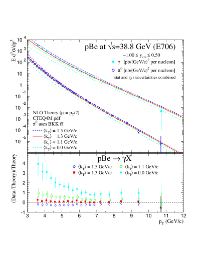
Figure 26: Data and Theory agree after $k_{T}$ smearing for $\pi^{0}$ and $\gamma$ production in pBe interactions at 800 GeV. Data-Theory/Theory comparison for various values of $k_{T}$ is shown in lower insert.

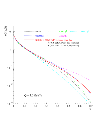
Figure 27: Recent PDF sets indicate substantial disagreement about the shape and size of gluon distribution at moderate to high x. CTEQ5 results closely follow CTEQ4M curve shown here.

A comparison of current gluon distribution parametrizations indicates our lack of knowledge of gluon in the moderate to high x range, (see Figure 27). The hardest gluon is the CTEQ4HJ distribution. Here the gluon distribution is forced to follow the high $E_{T}$ inclusive differential jet cross section measured at CDF. Latest PDF sets by CTEQ match the WA70 direct photon data at $\sqrt{(}s)$=23 GeV with no $k_{T}$, and require $k_{T}$=1.1 (1.3) GeV/c for the E706 data at $\sqrt{(}s)$=31 (38) GeV. Due to the difficulty in reconciling this approach no direct photon data is used in the CTEQ5 global analysis. The MRST group chose a different treatment: gluon distributions are reduced at high x to accommodate some $k_{T}$ smearing for both WA70 and E706 resulting in a moderately good description of the data and three PDF sets spanning the extremes (shown in Figure 27). The variety of predictions agree at low x, but differ widely at high x. The uncertainty in the $k_{T}$ modeling, its unknown shape versus $p_{T}$, and potential discrepancy between WA70 and E706 measurements (see discussions in [6] and [8]) require theoretical work to help resolve this outstanding controversy. Luckily, the interest in direct photon physics and its importance for gluon determination has caught on, and 98 and 99 have seen a flurry of publications, notably: “Soft-gluon resummation and NNLO corrections for direct photon production” by N. Kidonakis, J. Owens (hep-ph/9912388), “Results in next-to-leading-log prompt-photon hadroproduction” by S.Catani, M.Mangano, C.Oleari (hep-ph/9912206), “Unintegrated parton distributions and prompt photon hadroproduction” by M.Kimber, A.Martin, M.Ryskin (DTP/99/100), “Origin of $k_{T}$ smearing in direct photon production” by H.Lai, H.Li (hep-ph/9802414), “Sudakov resummation for prompt photon production in hadron collisions” by S.Catani, M.Mangano, P.Nason (hep-ph/9806484), etc. New resummation results are also expected from a group of G.Sterman and Vogelsang.

In addition to direct photons, the Tevatron jet and dijet measurements are also sensitive to the gluon distribution (in the moderate x region). These measurements and comparisons to theory have their own set of concerns, e.g. jet definition, which is never exactly the same in the data and in the NLO calculation or higher order correlations in the underlying event (see discussion in, e.g., [9]). The jet cross sections, strongly dominated by $q\bar{q}$ scattering, are also sensitive to changes in high x valence distributions. An unresolved issue in the jet cross section analysis is also a lack of full scaling between 630 and 1800 GeV data, predicted by QCD, and a discrepancy between the D0 and CDF measurements of this scaling ratio at lowest $x_{T}=E_{T}/\sqrt{(}s)$.

2.2 Valence distributions at high x

Apart from modifications to gluon and charm quark distributions, the valence d quark has received the biggest boost in high x region compared to previous PDF sets. The change is on the order of 30% at x=0.6 and $Q^{2}=20$GeV² and comes from inclusion of a new observable in the global analysis fits, namely W-lepton asymmetry measured at CDF. Precise measurement of W-lepton asymmetry serves as an independent check on the u and d quark distributions obtained from fits to deep inelastic data. The observable is directly correlated with the slope of the d/u ratio in the x range of 0.1-0.3. The consequence of this new constraint is that the predicted $F_{2}^{n}/F_{2}^{p}$ ratio is increased and the description of the NMC measurement of $F_{2}^{d}/F_{2}^{p}$ is improved relative to earlier PDF sets. There remain, however, two areas of uncertainty regarding valence distributions at high x: the value of d/u ratio at x=1 and a question regarding a need for nuclear corrections to $F_{2}^{d}/F_{2}^{p}$ NMC measurement. Deuterium is a loosely bound nucleus, of low A, and traditionally no corrections for nuclear effects have been applied. However, an analysis of SLAC $F_{2}$ data on different targets under the assumption that nuclear effects scale with the nuclear binding for all nuclei predicts nuclear correction for deuterium of 4$\pm$1% at x=0.7 [10]. There is also a lack of clarity regarding d/u value at 1. A non-perturbative QCD-motivated models of the 1970’s argue that the d/u ratio should approach 0.2 at highest x, whereas any standard form of the parametrization used in global fits drive this ratio to zero. The CTEQ collaboration has performed studies of change in d/u ratio, depending on assumptions regarding nuclear effects in deuterium and the value of d/u ratio at x=1 [3]. CTEQ5UD PDF set includes nuclear corrections for deuterium in $F_{2}^{d}/F_{2}^{p}$; its change relative to CTEQ5 is a plausible range for d distribution uncertainty in light of this unresolved question, see Figure 28.

Figure 28: The d/u ratio for CTEQ5 and CTEQ5UD PDF sets, illustrating difference from nuclear correction for NMC $F_{2}$ on deuterium. The dotted and dashed lines correspond to two different assumptions regarding value of d/u at x=1.

2.3 Resolved discrepancies between PDF fits and the data

During the duration of this Workshop (March - Nov 1999), two of the outstanding discrepancies between PDF fits or two sets of the experimental data have been resolved.

One of these was the near 20% discrepancy at small x (0.007-0.1) between structure function $F_{2}$ measured in muon (NMC) and neutrino (CCFR) deep inelastic scattering [11]. For the purpose of comparison of these structure functions, NMC $F_{2}^{\mu p}$ was “corrected” for nuclear shadowing, measured in muon scattering, to correspond to $F_{2}^{\mu Fe}$, and rescaled by the 5/18 charge rule to convert from muon to neutrino $F_{2}$. On the other hand, CCFR result was obtained in the framework of massless charm quark to avoid kinematic differences between muon and neutrino scattering off the strange quark ($\nu s\to\mu c$ versus $\mu s\to\mu s$) resulting from mass of the charm. Any one of the above procedures could have had an unquantified systematic uncertainty resulting in the observed disagreement.

New analysis from CCFR, presented at this Workshop [12], indicates that the SF measured in CCFR is in agreement with the $F_{2}$ of NMC, within experimental uncertainties. The analysis used a new measurement of the difference between neutrino and antineutrino structure functions $xF_{3}$, rather than the $\Delta xF_{3}$=4(s-c) parametrization used earlier. Comparison between calculations [13] indicated that there were large theoretical uncertainties in the charm production modeling for both $\Delta xF_{3}$ and the “slow rescaling” correction that converts from massive to massless charm quark framework. Therefore, in the new analysis “slow rescaling” correction was not applied and $\Delta xF_{3}$ and $F_{2}$ were extracted from two parameter fits to the data. The new measurement agrees well with the Mixed Flavor Scheme (MFS) for heavy quark production as implemented by MRST group. To compare with charged lepton scattering data each of the experimental results were divided by the theoretical predictions for $F_{2}$, using either light or heavy quark schemes implemented by MRST. The ratios of Data/Theory for $F_{2}^{\nu}$ (CCFR), $F_{2}^{\mu}$ (NMC), and $F_{2}^{e}$ (SLAC) are shown in Figure 29. Systematic errors, except for the overall normalization uncertainties, are included. The MFS MRST predictions have higher twist and target mass correction applied. Apart from resolving the NMC-CCFR discrepancy, the new measurement had also implication of ruling out one of the Variable Flavor Scheme calculations available on the market [14].

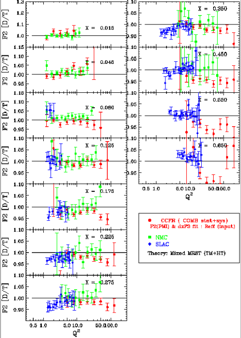
Figure 29: The ratio of the massive $F_{2}^{\nu}$ measured at CCFR to the prediction of MFS MRST prediction with target mass and higher twist corrections applied. Also shown are the ratios of $F_{2}{\mu}$ (NMC) and $F_{2}^{e}$ (SLAC) to the MFS MRST predictions.

Another example is that of Drell-Yan production ($pd\to\mu^{+}\mu^{-}$) as measured by Fermilab experiment E772, shown in Figure 30. The MRST fits are compared to the differential cross section in $x_{F}=x_{1}-x_{2}$ and in $\sqrt{(}\tau)=\sqrt{(}M^{2}/s)$, where $x_{1}$ and $x_{2}$ are the target and projectile fractional momenta, and $M$ - dimuon pair mass. The discrepancy, visible at high $x_{F}$ and low $\sqrt{(}\tau)$ was hard to reconcile, since in this kinematic region the dominant contribution to the cross section comes from $u(x_{1})\times[\bar{u}(x_{2})+\bar{d}(x_{2})]$ evaluated at $x_{1}\approx x_{F}$ and $x_{2}\approx$ 0.03, well constrained by the deep inelastic scattering data. Since then, the E772 experiment has reexamined their acceptance corrections and released an erratum to their earlier measurement [15]. The new values differ from the old ones only for large $x_{F}$ and small values of mass $M$, and the new cross section is decreased in this region by a factor up to two.

Figure 30: Drell-Yan production from E772 compared to the MRST prediction. The theory curves include K factor of 0.96 and the cross sections for different values of $x_{F}$ are offset by a factor of 10. Corrected E772 data reduce the discrepancy at high $x_{F}$ and low $\tau$.

3 Outlook for New Structure Function Measurements

Measurements of neutral and charged current cross sections in positron - proton collisions at large $Q^{2}$ from the 1994-97 data have just been published by HERA experiments [16][17]. The data sample corresponds to an integrated luminosity of 35 pb^-1. The $Q^{2}$ evolution of the parton densities of the proton is tested over 150-30000 GeV², Bjorken x between 0.0032-0.65, and yields no significant deviation from the prediction of perturbative QCD. These data samples are not yet sensitive eunough to pin down the d quark distribution at high x, however, an expected 1000 pb^-1 in positron and electron running in years 2001-2005, achievable after HERA luminosity upgrade, will have a lot to say about 20% -like effects at high x in the ratio of valence distributions.

HERA’s 1995-1999 data sets, not yet included in the global analysis fits, were ploted against standard PDFs and showed a good agreement over the new kinematic range that these data span (extention to lower yet x and higher $Q^{2}$ compared to 1994 data) [2]. HERA’s very large statistics and improved precision will allow further reduction of normalization uncertainty of PDF fits. This is important for QCD prediction like W and Z total cross sections at Tevatron - current 3% normalization uncertainty in PDFs directly translates to 3% uncertainty for these cross sections. Improvements in the measurements may need to go in hand with progress in the perturbative calculations; it is likely that NNLO analysis of deep inelastic scattering data will change the level and/or x dependence of PDFs at the percentish-type level.

One can expect continued progress in heavy quark treatment and in the theoretical understanding of soft gluon and non-perturbative effects in the direct photon production. In that case, the E706 data are sufficiently precise to severely constrain the gluon distribution.

One of the few currently active structure function – related experiments is also NuTeV (Fermilab E815). Better understanding of charm quark issues (see discussion in preceeding section) and much improved calibration of NuTeV detector relative to CCFR’s (with a similar statistical power of the data set) is expected to yield a more precise measurement of structure functions and differential cross section for $\nu$ and $\bar{\nu}$ interaction in Fe. Sign-selected beam and several advancements in the NLO theory of heavy quark production will allow NuTeV to improve systematic uncertainty in the new measurement of the strange seas $s$ and $\bar{s}$.

Last but not least, Run II physics promises to be a good source of new constraints on parton distributions. W-lepton asymmetry will be measured with much improved precision and in an expanded rapidity range. New observables are proposed for further exploring collider constrains on PDFs, e.g., W and Z rapidity distributions [18]. And hopefully, many of the issues in jet measurements will be addressed and understood – they are high on J.Wormesley Christmas wish-list! [19]

HEAVY QUARK PRODUCTION

R. Demina^a, S. Keller^b, M. Krämer^c, S. Kretzer^d, R. Martin^e, F.I. Olness^f, R.J. Scalise^f, D.E. Soper^g, W.-K. Tung^h,i, N. Varelas^e, and U.K. Yang^j.

a) Kansas State University, Physics Department, 116 Cardwell Hall, Manhattan, KS 66506; b) Theoretical Physics Division, CERN, CH-1211 Geneva 23, Switzerland; c) Department of Physics, University of Edinburgh, Edinburgh EH9 3JZ, Scotland; d) Univ. Dortmund, Dept. of Physics, D-44227 Dortmund, Germany; e) Univ. of Illinois at Chicago, Dept. of Physics, Chicago, IL 60607; f) Southern Methodist University, Department of Physics, Dallas, TX 75275-0175; g) Institute of Theoretical Science, University of Oregon, Eugene OR 97403, USA; h) Michigan State University, Department of Physics and Astronomy, East Lansing, Michigan 48824-1116; i) Fermi National Accelerator Laboratory, Batavia, IL 60510; j) University of Chicago, Enrico Fermi Institute, Chicago, IL 60637-1434.

Abstract

We present a status report of a variety of projects related to heavy quark production and parton distributions for the Tevatron Run II.

0.1 Introduction

The production of heavy quarks, both hadroproduction and leptoproduction, has become an important theoretical and phenomenological issue. While the hadroproduction mode is of direct interest to this workshop,[1] we shall find that the simpler leptoproduction process can provide important insights into the fundamental production mechanisms.[2, 3, 4, 5] Therefore, in preparation for the Tevatron Run II, we must consider information from a variety of sources including charm and bottom production at fixed-target and collider lepton and hadron facilities.

For example, the charm contribution to the total structure function $F_{2}$ at HERA, is sizeable, up to $\sim 25\%$ in the small $x$ region.[4] Therefore a proper description of charm-quark production is required for a global analysis of structure function data, and hence a precise extraction of the parton densities in the proton. These elements are important for addressing a variety of issues at the Tevatron.

In addition to the studies investigated at the Run II workshop series, we want to call attention to the extensive work done in the Standard Model Physics (and more) at the LHC Workshop organized by Guido Altarelli, Daniel Denegri, Daniel Froidevaux, Michelangelo Mangano, Tatsuya Nakada which was held at CERN during the same period. In particular, the investigations of the LHC b-production group (convenors: Paolo Nason, Giovanni Ridolfi, Olivier Schneider, Giuseppe Tartarelli, Vikas Pratibha) and the QCD group (convenors: Stefano Catani, Davison Soper, W. James Stirling, Stefan Tapprogge, Michael Dittmar) are directly relevant to the material discussed here. Furthermore, our report limits its scope to the issues discussed within the Run II workshop; for a recent comprehensive review, see Ref. [6].

0.2 Schemes for Heavy Quark Production

Heavy quark production also provides an important theoretical challenge as the presence of the heavy quark mass, $M$, introduces a new scale into the problem. The heavy quark mass scale, $M$, in addition to the characteristic energy scale of the process (which we will label here generically as $E$), will require a different organization of the perturbation series depending on the relative magnitudes of $M$ and $E$. We find there are essentially two cases to consider.

1. For the case of $E\sim M$, heavy-quark production is calculated in the so-called fixed flavor number (FFN) scheme from hard processes initiated by light quarks ($u,d,s$) and gluons, where all effects of the charm quark are contained in the perturbative coefficient functions. The FFN scheme incorporates the correct threshold behavior, but for large scales, $E\gg M$, the coefficient functions in the FFN scheme at higher orders in $\alpha_{s}$ contain potentially large logarithms $\ln^{n}(E^{2}/M^{2})$, which may need to be resummed.[7, 8, 9, 10]

2. For the case of $E\gg M$, it is necessary to include the heavy quark as an active parton in the proton. This serves to resum the potentially large logarithms $\ln^{n}(E^{2}/M^{2})$ discussed above. The simplest approach incorporating this idea is the so-called zero mass variable flavor number (ZM-VFN) scheme, where heavy quarks are treated as infinitely massive below some scale $E\sim M$ and massless above this threshold. This prescription has been used in global fits for many years, but it has an error of ${\cal O}(M^{2}/E^{2})$ and is not suited for quantitative analyses unless $E\gg M$.

While the extreme limits $E\gg M$ and $E\sim M$ are straightforward, much of the experimental data lie in the intermediate region As such, the correct PQCD formulation of heavy quark production, capable of spanning the full energy range, must incorporate the physics of both the FFN scheme and the ZM-VFN scheme. Considerable effort has been made to devise a prescription for heavy-flavor production that interpolates between the FFN scheme close to threshold and the ZM-VFN scheme at large $E$.

The generalized VFN scheme includes the heavy quark as an active parton flavor and involves matching between the FFN scheme with three active flavors and a four-flavor prescription with non-zero heavy-quark mass. It employs the fact that the mass singularities associated with the heavy-quark mass can be resummed into the parton distributions without taking the limit $M\to 0$ in the short-distance coefficient functions, as done in the ZM-VFN scheme. This is precisely the underlying idea of the Aivazis–Collins–Olness–Tung (ACOT) ACOT scheme[11] which is based on the renormalization method of Collins–Wilczek–Zee (CWZ).[12] The order-by-order procedure to implement this approach has now been systematically established to all orders in PQCD by Collins.[13]

Recently, additional implementations of VFN schemes have been defined in the literature. While these schemes all agree in principle on the result summed to all orders of perturbation theory, the way of ordering the perturbative expansion is not unique and the results differ at finite order in perturbation theory. The Thorne–Roberts (TR) [14] prescription has been used in the MRST recent global analyses of parton distributions.[15] The BMSN and CNS prescriptions have made use of the ${\cal O}(\alpha_{s}^{2})$ calculations by Smith, van Neerven, and collaborators[8, 9] to carry these ideas to higher order. The boundary conditions on the PDF’s at the flavor threshold become more complicated at this order; in particular, the PDF’s are no longer continuous across the N to N+1 flavor threshold. Buza et al.,[8] have computed the matching conditions, and this has been implemented in an evolution program by CSN.[9] More recently, a Simplified-ACOT (SACOT) scheme inspired by the prescription advocated by Collins [13] was introduced;[16] we describe this new scheme in Sec. 0.4.

0.3 From Low To High Energy Scale

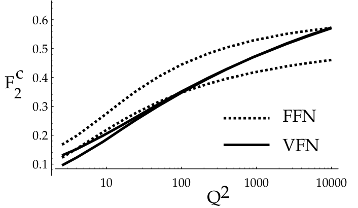
Figure 31: $F_{2}^{c}$ for $x=0.01$ as a function of $Q^{2}$ in GeV for two choices of $\mu$ as obtained within the ${\cal O}(\alpha_{s}^{1})$ FFN and (ACOT) VFN schemes. For details, see Ref. [17].

To compare the features of the FFN scheme with the ACOT VFN scheme concretely, we will take the example of heavy quark production in DIS; the features we extract from this example are directly applicable to the hadroproduction case relevant for the Tevatron Run II. One measure we have of estimating the uncertainty of a calculated quantity is to examine the variation of the renormalization and factorization scale dependence. While this method can only provide a lower bound on the uncertainty, it is a useful tool.

In Fig. 31, we display the component of $F_{2}^{c}$ for the $s+W\to c$ sub-process at $x=0.01$ plotted vs. $Q^{2}$. We gauge the scale uncertainty by varying $\mu$ from $1/2\,\mu_{0}$to $2.0\,\mu_{0}$ with $\mu_{0}=\sqrt{Q^{2}+m_{c}^{2}}$. In this figure, both schemes are applied to ${\cal O}(\alpha_{s}^{1})$. We observe that the FFN scheme is narrower at low $Q$, and increases slightly at larger $Q$. This behavior is reasonable given that we expect this scheme to work best in the threshold region, but to decrease in accuracy as the unresummed logs of $\ln^{n}(Q^{2}/m_{c}^{2})$ increase.

Conversely, the ACOT VFN scheme has quite the opposite behavior. At low $Q$, this calculation displays mild scale uncertainty, but at large $Q$ this uncertainty is significantly reduced. This is an indication that the resummation of the $\ln^{n}(Q^{2}/m_{c}^{2})$ terms via the heavy quark PDF serves to decrease the scale uncertainty at a given order of perturbation theory. While these general results were to be expected, what is surprising is the magnitude of the scale variation. Even in the threshold region where $Q\sim m_{c}$ we find that the VFN scheme is comparable or better than the FFN scheme.

At present, the FFN scheme has been calculated to one further order in perturbation theory, ${\cal O}(\alpha_{s}^{2})$. While the higher order terms do serve to reduce the scale uncertainty, it is only at the lowest values of $Q$ that the ${\cal O}(\alpha_{s}^{2})$ FFN band is smaller than the ${\cal O}(\alpha_{s}^{1})$ VFN band. Recently, ${\cal O}(\alpha_{s}^{2})$ calculations in the VFN scheme have been performed;[9] it would be interesting to extend such comparisons to these new calculations.

Let us also take this opportunity to clarify a misconception that has occasionally appeared in the literature. The VFN scheme is not required to reduce to the FFN scheme at $Q=m_{c}$. While it is true that the VFN scheme does have the FFN scheme as a limit, this matching depends on the definitions of the PDF’s, and the choice of the $\mu$ scale. In this particular example, even at $Q=m_{c}$, the resummed logs in the heavy quark PDF can yield a non-zero contribution which help to stabilize the scale dependence of the VFN scheme result.

The upshot is that even in the threshold region, the resummation of the logarithms via the heavy quark PDF’s can help the stability of the theory.

0.4 Simplified ACOT (SACOT) prescription

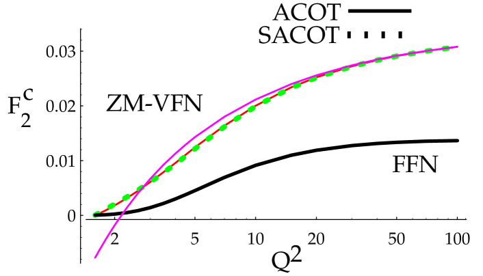
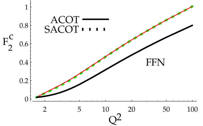
Figure 32: $F_{2}^{c}$ as a function of $Q^{2}$ in GeV computed to ${\cal O}(\alpha_{s}^{1})$ in the ZM-VFN, FFN, ACOT, and SACOT schemes using CTEQ4M PDF’s. Fig. a) $x=0.1$ , and Fig. b) $x=0.001$. Figures taken from Ref. [16].

We investigate a modification of the ACOT scheme inspired by the prescription advocated by Collins.[13] This prescription has the advantage of being easy to state, and allowing relatively simple calculations. Such simplicity could be crucial for going beyond one loop order in calculations.

Simplified ACOT (SACOT) prescription. Set $M_{H}$ to zero in the calculation of the hard scattering partonic functions $\widehat{\sigma}$ for incoming heavy quarks.

For example, this scheme tremendously simplifies the calculation of the neutral current structure function $F_{2}^{charm}$ even at ${\cal O}(\alpha_{s}^{1})$. In other prescriptions, the tree process $\gamma+c\to c+g$ and the one loop process $\gamma+c\to c$ must be computed with non-zero charm mass, and this results in a complicated expression.[20] In the SACOT scheme, the charm mass can be set to zero so that the final result for these sub-processes reduces to the very simple massless result.

While the SACOT scheme allows us to simplify the calculation, the obvious question is: does this simplified version contain the full dynamics of the process. To answer this quantitatively, we compare prediction for $F_{2}^{charm}$ obtained with 1) the SACOT scheme at order $\alpha_{s}^{1}$ with 2) the predictions obtained with the original ACOT scheme, 3) the ZM-VFN procedure in which the charm quark can appear as a parton but has zero mass, and 4) the FFN procedure in which the charm quark has its proper mass but does not appear as a parton. For simplicity, we take $\mu=Q$.

In Fig. 32 we show $F_{2}^{c}(x,Q)$ as a function of $Q$ for $x=0.1$ and $x=0.001$ using the CTEQ4M parton distributions.[21, 22] We observe that the ACOT and SACOT schemes are effectively identical throughout the kinematic range. There is a slight difference observed in the threshold region, but this is small in comparison to the renormalization/factorization $\mu$-variation (not shown). Hence the difference between the ACOT and SACOT results is of no physical consequence. The fact that the ACOT and SACOT match extremely well throughout the full kinematic range provides explicit numerical verification that the SACOT scheme fully contains the physics.

Although we have used the example of heavy quark leptoproduction, let us comment briefly on the implications of this scheme for the more complex case of hadroproduction.[1, 23, 24, 25] At present, we have calculations for the all the ${\cal O}(\alpha_{s}^{2})$ hadroproduction sub-processes such as $gg\to Q\bar{Q}$ and $gQ\to gQ$. At ${\cal O}(\alpha_{s}^{3})$ we have the result for the $gg\to gQ\bar{Q}$ sub-processes, but not the general result for $gQ\to ggQ$ with non-zero heavy quark mass. With the SACOT scheme, we can set the heavy quark mass to zero in the $gQ\to ggQ$ sub-process and thus make use of the simple result already in the literature. This is just one example of how the SACOT has the practical advantage of allowing us to extend our calculations to higher orders in the perturbation theory. We now turn to the case of heavy quark production for hadron colliders.

0.5 Heavy Quark Hadroproduction

Figure 33: Differential cross section for b-production vs. $p_{T}$ comparing the Fixed-Order (FO) and the Fixed-Order Next-to-Leading-Log (FONLL) result in the $\overline{MS}$ scheme. The bands are obtained by varying independently the renormalization and factorization scales. The cross section is scaled by $m_{T}^{5}$ with $m_{T}=\sqrt{m_{b}^{2}+p_{T}^{2}}$, and $\sqrt{s}=1800\,GeV$, $m_{b}=5\,GeV$, $y=0$, with CTEQ3M PDF’s. Figure taken from Cacciari, Greco, and Nason, Ref. [27].

There has been notable progress in the area of hadroproduction of heavy quarks. The original NLO calculations of the $gg\to b\bar{b}$ subprocess were performed by Nason, Dawson, and Ellis [23], and by Beenakker, Kuijf, van Neerven, Meng, Schuler, and Smith[24]. Recently, Cacciari and Greco[26] have used a NLO fragmentation formalism to resum the heavy quark contributions in the limit of large $p_{T}$; the result is a decreased renormalization/factorization scale variation in the large $p_{T}$ region. The ACOT scheme was applied to the hadroproduction case by Olness, Scalise, and Tung.[25] More recently, the NLO fragmentation formalism of Cacciari and Greco has been merged with the massive FFN calculation of Nason, Dawson, and Ellis by Cacciari, Greco, and Nason,[27]; the result is a calculation which matches the FFN calculation at low $p_{T}$, and takes advantage of the NLO fragmentation formalism in the high $p_{T}$ region, thus yielding good behavior throughout the full $p_{T}$ range. This is displayed in Fig. 33 where we see that this Fixed-Order Next-to-Leading-Log (FONLL) calculation displays reduced scale variation in the large $p_{T}$ region, and matches on the the massive NLO calculation in the small $p_{T}$ region. Further details can be found in the report of the LHC Workshop b-production group.

0.6 $W$ + Heavy Quark Production

PDF Set	Mass (GeV)	LO	$WQ\bar{Q}$	NLO
CTEQ1M	$m_{c}$=1.7	96	20	161
MRSD0’	$m_{c}$=1.7	81	20	138
CTEQ3M	$m_{c}$=1.7	83	20	141
CTEQ3M	$m_{b}$=5.0	0.17	9.09	9.33

Table 3: The $W$ + charm-tagged one-jet inclusive cross section in $pb$ for LO, $W+Q\bar{Q}$, and NLO (including the $W+Q\bar{Q}$ contribution) using different sets of parton distribution functions. Table is taken from Ref. [28].

Figure 34: Differential $d\sigma/dp_{T}^{\gamma}$ for $\gamma$ plus tagged heavy quark production as compared with Pythia and the NLO QCD results. Figure taken from Ref. [29]. NLO QCD calculations from Ref. [30].

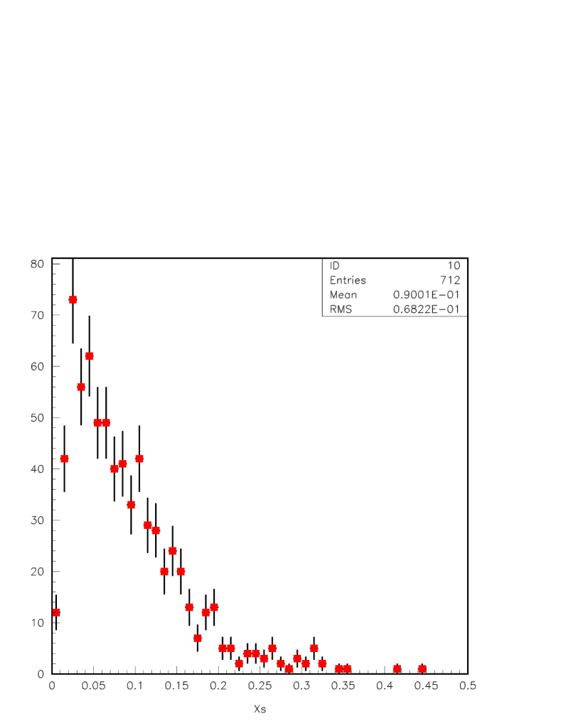
Figure 35: Distribution of $Events/0.01$ vs. $x$ of the s-quarks which contribute to the $s+W\to c$ process. Figure taken from Ref. [31].

The precise measurement of $W$ plus heavy quark ($W$+$Q$) events provides an important information on a variety of issues. Measurement of $W$+$Q$ allows us to test NLO QCD theory at high scales and investigate questions about resummation and heavy quark PDF’s. For example, if sufficient statistics are available, $W$+$charm$ final states can be used to extract information about the strange quark distribution. In an analogous manner, the $W$+$bottom$ final states are sensitive to the charm PDF; furthermore, $W$+$bottom$ can fake Higgs events, and are also an important background for sbottom ($\widetilde{b}$) searches.

The cross sections for $W$ plus tagged heavy quark jet were computed in Ref. [28], and are shown in Table. 3. Note that this process has a large $K$-factor, and hence comparison between data and theory will provide discerning test of the NLO QCD theory. While the small cross sections of these channels hindered analysis in Run I, the increased luminosity in Run II can make this a discriminating tool. For example, Run I provided minimal statistics on $W$+$Q$, but there was data in the analogous neutral current channel $\gamma$+$Q$. The NLO QCD cross sections for $\gamma$ plus heavy quark were computed in Ref. [30]. Fig. 34 displays preliminary Tevatron data from Run I and the comparison with both the PYTHIA Monte Carlo and the NLO QCD calculations; again, note the large $K$-factor. If similar results are attainable in the charged current channel at Run II, this would be revealing.

Extensive analysis the $W$+$Q$ production channels were performed in Working Group I: “QCD tools for heavy flavors and new physics searches,” and we can make use of these results to estimate the precision to which the strange quark distribution can be extracted. We display Fig. 35 (taken from the WGI report[31]) which shows the distribution in $x$ of the s-quarks which contribute to the $W$+$c$ process. This figure indicates that there will good statistics in an $x$-range comparable to that investigated by neutrino DIS experiments;[2, 3] hence, comparison with this data should provide an important test of the strange quark sea and the underlying mechanisms for computing such processes.

0.7 The Strange Quark Distribution

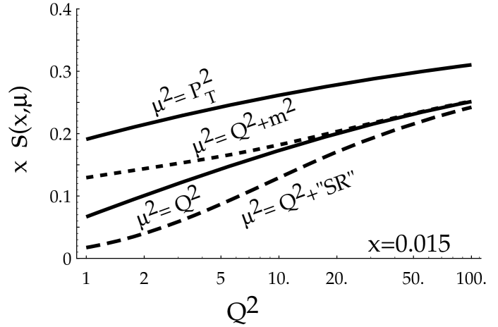
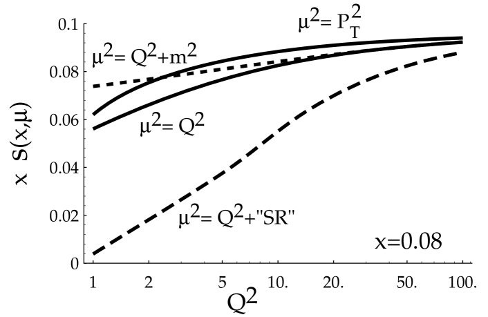
Figure 36: Variation of $x\,s(x,\mu)$ for three choices of $\mu$, and also with a “SR” (slow-rescaling) type correction: $x\to x(1+m_{c}^{2}/Q^{2})$.

Figure 37: $\Delta xF_{3}/2$ vs. $Q^{2}$ for three choices of $x$. Calculations provided by S. Kretzer.

A primary uncertainty for $W$+$charm$ production discussed above comes from the strange sea PDF, $s(x)$, which has been the subject of controversy for sometime now. One possibility is that new analysis of present data will resolve this situation prior to Run II, and provide precise distributions as an input the the Tevatron data analysis. The converse would be that this situation remains unresolved, in which case new data from Run II may help to finally solve this puzzle.

The strange distribution is directly measured by dimuon production in neutrino-nucleon scattering. The basic sub-process is $\nu N\to\mu^{-}cX$ with a subsequent charm decay $c\to\mu^{+}X^{\prime}$.

The strange distribution can also be extracted indirectly using a combination of charged ($W^{\pm}$) and neutral ($\gamma$) current data; however, the systematic uncertainties involved in this procedure make an accurate determination difficult.[32] The basic idea is to use the relation

$$\frac{F_{2}^{NC}}{F_{2}^{CC}}=\frac{5}{18}\left\{1-\frac{3}{5}\,\frac{(s+\bar{s})-(c+\bar{c})+...}{q+\bar{q}}\right\}$$ (48)

to extract the strange distribution. This method is complicated by a number of issues including the $xF_{3}$ component which can play a crucial role in the small-$x$ region—precisely the region where there has been a long-standing discrepancy.

The structure functions are defined in terms of the neutrino-nucleon cross section via:

$$\frac{d^{2}\sigma^{\nu,\bar{\nu}}}{dx\,dy}=\frac{\scriptstyle G_{F}^{2}ME}{\pi}\left[F_{2}(1-y)+xF_{1}y^{2}\pm xF_{3}y(1-\frac{y}{2})\right]$$

It is instructive to recall the simple leading-order correspondence between the $F$’s and the PDF’s:

$$F_{2}^{(\nu,\bar{\nu})N} = x\left\{u+\bar{u}+d+\bar{d}+2s+2c\right\}$$

$$xF_{3}^{(\nu,\bar{\nu})N} = x\left\{u-\bar{u}+d-\bar{d}\pm 2s\mp 2c\right\}$$ (49)

Therefore, the combination $\Delta xF_{3}$:

$$\Delta xF_{3}=xF_{3}^{\nu N}-xF_{3}^{\bar{\nu}N}=4x\{s-c\}$$ (50)

can be used to probe the strange sea distribution, and to understand heavy quark (charm) production. This information, together with the exclusive dimuon events, may provide a more precise determination of the strange quark sea.

To gauge the dependence of $\Delta xF_{3}$ upon various factors, we first consider $xs(x,\mu)$ in Fig. 36, and then the full NLO $\Delta xF_{3}$ in Fig. 37; this allows us to see the connection between $\Delta xF_{3}$ and $xs(x,\mu)$ beyond leading order. In Fig. 36 we have plotted the quantity $xs(x,\mu)$ vs. $Q^{2}$ for two choices of $x$ in a range relevant to the the dimuon measurements. We use three choices of the $\mu^{2}$ scale: $\{Q^{2},Q^{2}+m_{c}^{2},P_{T_{max}}^{2}\}$. The choices $Q^{2}$ and $Q^{2}+m_{c}^{2}$ differ only at lower values of $Q^{2}$; the choice $P_{T_{max}}^{2}$ is comparable to $Q^{2}$ and $Q^{2}+m_{c}^{2}$ at $x=0.08$ but lies above for $x=0.015$. The fourth curve labeled $Q^{2}+``SR"$ uses $\mu^{2}=Q^{2}$ with a “slow-rescaling” type of correction which (crudely) includes mass effects by shifting $x$ to $x(1+m_{c}^{2}/Q^{2})$; note, the result of this correction is significant at large $x$ and low $Q^{2}$.

In Fig. 37 we have plotted the quantity $\Delta xF_{3}/2$ for an isoscalar target computed to order $\alpha_{s}^{1}$. We display three calculations for three different $x$-bins relevant to strange sea measurement. 1) A 3-flavor calculation using the GRV98[33] distributions, and $\mu=\sqrt{Q^{2}+m^{2}}$. 2) A 3-flavor calculation using the CTEQ4HQ distributions, and $\mu=Q$. 3) A 4-flavor calculation using the CTEQ4HQ distributions, and $\mu=Q$.

The two CTEQ curves show the effect of the charm distribution, and the GRV curve shows the effect of using a different PDF set. Recall that the GRV calculation corresponds to a FFN scheme.

The pair of curves using the CTEQ4HQ distributions nicely illustrates how the charm distribution $c(x,\mu^{2})$ evolves as $\ln(Q^{2}/m_{c}^{2})$ for increasing $Q^{2}$; note, $c(x,\mu^{2})$ enters with a negative sign so that the 4-flavor result is below the 3-flavor curve. The choice $\mu=Q$ ensures the 3- and 4-flavor calculation coincide at $\mu=Q=m_{c}$; while this choice is useful for instructive purposes, a more practical choice might be $\mu\sim\sqrt{Q^{2}+m^{2}}$, cf., Sec. 0.2, and Ref. [17].

For comparison, we also display preliminary data from the CCFR analysis.[32] While there is much freedom in the theoretical calculation, the difference between these calculations and the data at low $Q$ values warrants further investigation.

0.8 Conclusions and Outlook

A detailed understanding of heavy quark production and heavy quark PDF’s at the Tevatron Run II will require analysis of fixed-target and HERA data as well as Run I results. Comprehensive analysis of the combined data set can provide incisive tests of the theoretical methods in an unexplored regime, and enable precise predictions that will facilitate new particle searches in a variety of channels. This document serves as a progress report, and work on these topics will continue in preparation for the Tevatron Run II.

This work is supported by the U.S. Department of Energy, the National Science Foundation, and the Lightner-Sams Foundation.

PARTON DENSITIES FOR HEAVY QUARKS

J. Smith

C.N. Yang Institute for Theoretical Physics, SUNY at Stony Brook , Stony Brook, NY 11794-3840)

Abstract

We compare parton densities for heavy quarks.

Reactions with incoming heavy (c,b) quarks are often calculated with heavy quark densities just like those with incoming light mass (u,d,s) quarks are calculated with light quark densities. The heavy quark densities are derived within the framework of the so-called zero-mass variable flavor number scheme (ZM-VFNS). In this scheme these quarks are described by massless densities which are zero below a specific mass scale $\mu$. The latter depends on $m_{c}$ or $m_{b}$. Let us call this scale the matching point. Below it there are $n_{f}$ massless quarks described by $n_{f}$ massless densities. Above it there are $n_{f}+1$ massless quarks described by $n_{f}+1$ massless densities. The latter densities are used to calculate processes with a hard scale $M\gg m_{c},m_{b}$. For example in the production of single top quarks via the weak process $q_{i}+b\rightarrow q_{j}+t$, where $q_{i}$, $q_{j}$ are light mass quarks in the proton/antiproton, one can argue that $M=m_{t}$ should be chosen as the large scale and $m_{b}$ can be neglected. Hence the incoming bottom quark can be described by a massless bottom quark density.

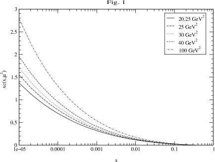
Figure 38: The charm quark density $xc_{\rm NNLO}(5,x,\mu^{2})$ in the range $10^{-5}<x<1$ for $\mu^{2}=$ 20.25, 25, 30, 40 and 100 in units of $({\rm GeV/c}^{2})^{2}$.

The generation of these densities starts from the solution of the evolution equations for $n_{f}$ massless quarks below the matching point. At and above this point one solves the evolution equations for $n_{f}+1$ massless quarks. However in contrast to the parameterization of the $x$-dependences of the light quarks and gluon at the initial starting scale, the $x$ dependence of the heavy quark density at the matching point is fixed. In perturbative QCD it is defined by convolutions of the densities for the $n_{f}$ quarks and the gluon with specific operator matrix elements (OME’s), which are now know up to $O(\alpha_{s}^{2})$ [1]. These matching conditions determine both the ZM-VFNS density and the other light-mass quark and gluon densities at the matching points. Then the evolution equations determine the new densities at larger scales. The momentum sum rule is satisfied for the $n_{f}+1$ quark densities together with the corresponding gluon density.

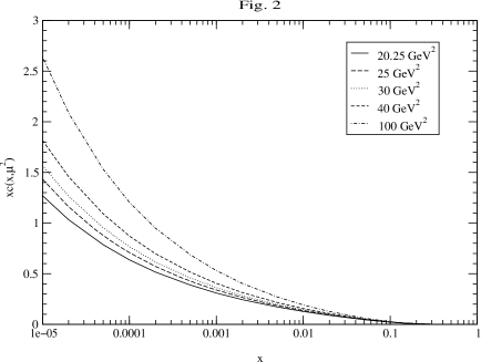
Figure 39: Same as Fig.1 for the NLO results from MRST98 set 1.

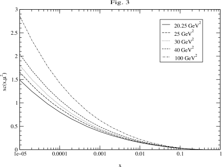
Figure 40: Same as Fig.1 for the NLO results from CTEQ5HQ.

Parton density sets contain densities for charm and bottom quarks, which generally directly follow this approach or some modification of it. The latest CTEQ densities [2] use $O(\alpha_{s})$ matching conditions. The $x$ dependencies of the heavy c and b-quark densities are zero at the matching points. The MRST densities [3] have more complicated matching conditions designed so that the derivatives of the deep inelastic structure functions $F_{2}$ and $F_{L}$ with regard to $Q^{2}$ are continuous at the matching points. Recently we have provided another set of ZM-VFNS densities [4], which are based on extending the GRV98 three-flavor densities in [5] to four and five-flavor sets. GRV give the formulae for their LO and NLO three flavor densities at very small scales. They never produced a c-quark density but advocated that charm quarks should only exist in the final state of production reactions, which should be calculated from NLO QCD with massive quarks as in [6]. We have evolved their LO and NLO densities across the matching point $\mu=m_{c}$ with $O(\alpha_{s}^{2})$ matching conditions to provide LO and NLO four-flavor densities containing massless c-quark densities. Then these LO and NLO densities were evolved between $\mu=m_{c}$ and $\mu=m_{b}$ with four-flavor LO and NLO splitting functions. At this new matching point the LO and NLO four-flavor densities were then convoluted with the $O(\alpha_{s}^{2})$ OME’s to form five-flavor sets containing massless b-quarks. These LO and NLO densities were then evolved to higher scales with five-flavor LO and NLO splitting functions. Note that the $O(\alpha_{s}^{2})$ matching conditions should really be used with NNLO splitting functions to produce NNLO density sets. However the latter splitting functions are not yet available, so we make the approximation of replacing the NNLO splitting functions with NLO ones.

Figure 41: The bottom quark density $xb_{\rm NNLO}(5,x,\mu^{2})$ in the range $10^{-5}<x<1$ for $\mu^{2}=$ 20.25, 25, 30, 40 and 100 in units of $({\rm GeV/c}^{2})^{2}$.

In this short report we would like to compare the charm and bottom quark densities in the CS, MRS and CTEQ sets. We concentrate on the five-flavor densities, which are more important for Tevatron physics. In the CS set they start at $\mu^{2}=m_{b}^{2}=20.25$ ${\rm GeV}^{2}$. At this scale the charm densities in the CS, MRST98 (set 1) and CTEQ5HQ sets are shown in Figs.1,2,3 respectively. Since the CS charm density starts off negative for small $x$ at $\mu^{2}=m_{c}^{2}=1.96$ ${\rm GeV}^{2}$ it evolves less than the corresponding CTEQ5HQ density. At larger $\mu^{2}$ all the CS curves in Fig.1 are below those for CTEQ5HQ in Fig.3 although the differences are small. In general the CS c-quark densities are more equal to those in the MRST (set 1) in Fig.2.

Figure 42: Same as Fig.4 for the NLO results from MRST98 set 1.

At the matching point $\mu^{2}=20.25$ ${\rm GeV}^{2}$ the b-quark density also starts off negative at small $x$ as can be seen in Fig.4, which is a consequence of the explicit form of the OME’s in [1]. At $O(\alpha_{s}^{2})$ the OME’s have nonlogarithmic terms which do not vanish at the matching point and yield a finite function in $x$, which is the boundary value for the evolution of the b-quark density. This negative start slows down the evolution of the b-quark density at small $x$ as the scale $\mu^{2}$ increases. Hence the CS densities at small $x$ in Fig.4 are smaller than the MRST98 (set 1) densities in Fig.5 and the CTEQ5HQ densities in Fig.6 at the same values of $\mu^{2}$. The differences between the sets are still small, of the order of five percent at small $x$ and large $\mu^{2}$. Hence it should not really matter which set is used to calculate cross sections for processes involving incoming b-quarks at the Tevatron.

Figure 43: Same as Fig.4 for the NLO results from CTEQ5HQ.

We suspect that the differences between these results for the heavy c and b-quark densities are primarily due to the different gluon densities in the three sets rather to than the effects of the different boundary conditions. This could be checked theoretically if both LO and NLO three-flavor sets were provided by MRST and CTEQ at small scales. Then we could rerun our programs to generate sets with $O(\alpha_{s}^{2})$ boundary conditions. However these inputs are not available. We note that CS uses the GRV98 LO and NLO gluon densities, which are rather steep in $x$ and generally larger than the latter sets at the same values of $\mu^{2}$. Since the discontinuous boundary conditions suppress the charm and bottom densities at small $x$, they enhance the gluon densities in this same region (in order that the momentum sum rules are satisfied). Hence the GRV98 three flavour gluon densities and the CS four and five flavor gluon densities are generally significantly larger than those in MRST98 (set 1) and CTEQ5HQ. Unfortunately experimental data are not yet precise enough to decide which set is the best one. We end by noting that all these densities are given in the $\overline{\rm MS}$ scheme.

CONSTRAINTS ON THE GLUON DENSITY FROM LEPTON PAIR PRODUCTION

E. L. Berger^a, and M. Klasen^b,.

a) HEP Theory Group, Argonne National Laboratory, 9700 South Cass Avenue, Argonne, IL 60439,USA; b) II. Institut für Theoretische Physik, Universität Hamburg, Luruper Chaussee 149, D-22761 Hamburg, Germany

Abstract

The hadroproduction of lepton pairs with mass $Q$ and finite transverse momentum $Q_{T}$ is described in perturbative QCD by the same partonic subprocesses as prompt photon production. We demonstrate that, like prompt photon production, lepton pair production is dominated by quark-gluon scattering in the region $Q_{T}>Q/2$. This feature leads to sensitivity to the gluon density in kinematical regimes accessible in collider and fixed target experiments, and it provides a new independent method for constraining the gluon density.

1 Introduction

The production of lepton pairs in hadron collisions $h_{1}h_{2}\rightarrow\gamma^{*}X;\gamma^{*}\rightarrow l\bar{l}$ proceeds through an intermediate virtual photon via $q{\bar{q}}\rightarrow\gamma^{*}$, and the subsequent leptonic decay of the virtual photon. Traditionally, interest in this Drell-Yan process has concentrated on lepton pairs with large mass $Q$ which justifies the application of perturbative QCD and allows for the extraction of the antiquark density in hadrons [1].

Prompt photon production $h_{1}h_{2}\rightarrow\gamma X$ can be calculated in perturbative QCD if the transverse momentum $Q_{T}$ of the photon is sufficiently large. Because the quark-gluon Compton subprocess is dominant, $gq\rightarrow\gamma X$, this reaction provides essential information on the gluon density in the proton at large $x$ [2]. Unfortunately, the analysis suffers from fragmentation, isolation, and intrinsic transverse momentum uncertainties. Alternatively, the gluon density can be constrained from the production of jets with large transverse momentum at hadron colliders [3], but the information from different experiments and colliders is ambiguous.

In this paper we demonstrate that, like prompt photon production, lepton pair production is dominated by quark-gluon scattering in the region $Q_{T}>Q/2$. This realization means that new independent constraints on the gluon density may be derived from Drell-Yan data in kinematical regimes that are accessible in collider and fixed target experiments but without the theoretical and experimental uncertainties present in the prompt photon case.

In Sec. 2, we review the relationship between virtual and real photon production in hadron collisions in next-to-leading order QCD. In Sec. 3 we present our numerical results, and Sec. 4 is a summary.

2 Next-to-leading order qcd formalism

In leading order (LO) QCD, two partonic subprocesses contribute to the production of virtual and real photons with non-zero transverse momentum: $q\bar{q}\rightarrow\gamma^{(*)}g$ and $qg\rightarrow\gamma^{(*)}q$. The cross section for lepton pair production is related to the cross section for virtual photon production through the leptonic branching ratio of the virtual photon $\alpha/(3\pi Q^{2})$. The virtual photon cross section reduces to the real photon cross section in the limit $Q^{2}\rightarrow 0$.

The next-to-leading order (NLO) QCD corrections arise from virtual one-loop diagrams interfering with the LO diagrams and from real emission diagrams. At this order $2\rightarrow 3$ partonic processes with incident gluon pairs $(gg)$, quark pairs $(qq)$, and non-factorizable quark-antiquark $(q\bar{q}_{2})$ processes contribute also. Singular contributions are regulated in $n$=4-2$\epsilon$ dimensions and removed through $\overline{\rm MS}$ renormalization, factorization, or cancellation between virtual and real contributions. An important difference between virtual and real photon production arises when a quark emits a collinear photon. Whereas the collinear emission of a real photon leads to a $1/\epsilon$ singularity that has to be factored into a fragmentation function, the collinear emission of a virtual photon yields a finite logarithmic contribution since it is regulated naturally by the photon virtuality $Q$. In the limit $Q^{2}\rightarrow 0$ the NLO virtual photon cross section reduces to the real photon cross section if this logarithm is replaced by a $1/\epsilon$ pole. A more detailed discussion can be found in [4].

The situation is completely analogous to hard photoproduction where the photon participates in the scattering in the initial state instead of the final state. For real photons, one encounters an initial-state singularity that is factored into a photon structure function. For virtual photons, this singularity is replaced by a logarithmic dependence on the photon virtuality $Q$ [5].

A remark is in order concerning the interval in $Q_{T}$ in which our analysis is appropriate. In general, in two-scale situations, a series of logarithmic contributions will arise with terms of the type $\alpha_{s}^{n}\ln^{n}(Q/Q_{T})$. Thus, if either $Q_{T}>>Q$ or $Q_{T}<<Q$, resummations of this series must be considered. For practical reasons, such as event rate, we do not venture into the domain $Q_{T}>>Q$, and our fixed-order calculation should be adequate. On the other hand, the cross section is large in the region $Q_{T}<<Q$. In previous papers [4], we compared our cross sections with available fixed-target and collider data on massive lepton-pair production, and we were able to establish that fixed-order perturbative calculations, without resummation, should be reliable for $Q_{T}>Q/2$. At smaller values of $Q_{T}$, non-perturbative and matching complications introduce some level of phenomenological ambiguity. For the goal we have in mind, viz., contraints on the gluon density, it would appear best to restrict attention to the region $Q_{T}\geq Q/2$, but below $Q_{T}>>Q$.

3 Predicted cross sections

In this section we present numerical results for the production of lepton pairs in $p\bar{p}$ collisions at the Tevatron with center-of mass energy $\sqrt{S}=1.8$ and 2.0 TeV. We analyze the invariant cross section $Ed^{3}\sigma/dp^{3}$ averaged over the rapidity interval -1.0 $<y<$ 1.0. We integrate the cross section over various intervals of pair-mass $Q$ and plot it as a function of the transverse momentum $Q_{T}$. Our predictions are based on a NLO QCD calculation [6] and are evaluated in the $\overline{\rm MS}$ renormalization scheme. The renormalization and factorization scales are set to $\mu=\mu_{f}=\sqrt{Q^{2}+Q_{T}^{2}}$. If not stated otherwise, we use the CTEQ4M parton distributions [7] and the corresponding value of $\Lambda$ in the two-loop expression of $\alpha_{s}$ with four flavors (five if $\mu>m_{b}$). The Drell-Yan factor $\alpha/(3\pi Q^{2})$ for the decay of the virtual photon into a lepton pair is included in all numerical results.

In Fig. 44 we display the NLO QCD cross section for lepton pair

Figure 44: Invariant cross section $Ed^{3}\sigma/dp^{3}$ as a function of $Q_{T}$ for $p\bar{p}\rightarrow\gamma^{*}X$ at $\sqrt{S}=1.8$ TeV in non-resonance regions of $Q$. The cross section falls with the mass of the lepton pair $Q$ and, more steeply, with its transverse momentum $Q_{T}$.

production at the Tevatron at $\sqrt{S}=1.8$ TeV as a function of $Q_{T}$ for four regions of $Q$. The regions of $Q$ have been chosen to avoid resonances, i.e.  between $2$ GeV and the $J/\psi$ resonance, between the $J/\psi$ and the $\Upsilon$ resonances, above the $\Upsilon$’s, and a high mass region. The cross section falls both with the mass of the lepton pair $Q$ and, more steeply, with its transverse momentum $Q_{T}$. No data are available yet from the CDF and D0 experiments. However, prompt photon production data exist to $Q_{T}\simeq 100$ GeV, where the cross section is about $10^{-3}$ pb/GeV². It should be possible to analyze Run I data for lepton pair production to at least $Q_{T}\simeq 30$ GeV where one can probe the parton densities in the proton up to $x_{T}=2Q_{T}/\sqrt{S}\simeq 0.03$. The UA1 collaboration measured the transverse momentum distribution of lepton pairs at $\sqrt{S}=630$ GeV up to $x_{T}=0.13$ [8], and their data agree well with our theoretical results [4].

The fractional contributions from the $qg$ and $q\bar{q}$ subprocesses through NLO are shown in Fig. 45. It is evident

Figure 45: Contributions from the partonic subprocesses $qg$ and $q\bar{q}$ to the invariant cross section $Ed^{3}\sigma/dp^{3}$ as a function of $Q_{T}$ for $p\bar{p}\rightarrow\gamma^{*}X$ at $\sqrt{S}$ = 1.8 TeV. The $qg$ channel dominates in the region $Q_{T}>Q/2$.

that the $qg$ subprocess is the most important subprocess as long as $Q_{T}>Q/2$. The dominance of the $qg$ subprocess diminishes somewhat with $Q$, dropping from over 80 % for the lowest values of $Q$ to about 70 % at its maximum for $Q\simeq$ 30 GeV. In addition, for very large $Q_{T}$, the significant luminosity associated with the valence dominated $\bar{q}$ density in $p\bar{p}$ reactions begins to raise the fraction of the cross section attributed to the $q\bar{q}$ subprocesses. Subprocesses other than those initiated by the $q\bar{q}$ and $qg$ initial channels are of negligible import.

We update the Tevatron center-of-mass energy to Run II conditions ($\sqrt{S}=2.0$ TeV) and use the latest global fit by the CTEQ collaboration (5M). Figure 46

Figure 46: Invariant cross section $Ed^{3}\sigma/dp^{3}$ as a function of $Q_{T}$ for $p\bar{p}\rightarrow\gamma^{*}X$ and two different center-of-mass energies of the Tevatron (Run 1: $\sqrt{S}=1.8$ TeV, Run 2: $\sqrt{S}=2.0$ TeV). The cross section for Run 2 is 5 to 20 % larger, depending on $Q_{T}$.

demonstrates that the larger center-of-mass energy increases the invariant cross section for the production of lepton pairs with mass 5 GeV $<Q<$ 6 GeV by 5 % at low $Q_{T}\simeq 1$ GeV and 20 % at high $Q_{T}\simeq 100$ GeV. In addition, the expected luminosity for Run II of 2 fb^-1 should make the cross section accessible to $Q_{T}\simeq 100$ GeV or $x_{T}\simeq 0.1$. This extension would constrain the gluon density in the same regions as prompt photon production in Run I.

Next we present a study of the sensitivity of collider and fixed target experiments to the gluon density in the proton. The full uncertainty in the gluon density is not known. Here we estimate this uncertainty from the variation of different recent parametrizations. We choose the latest global fit by the CTEQ collaboration (5M) as our point of reference [3] and compare results to those based on their preceding analysis (4M[7]) and on a fit with a higher gluon density (5HJ) intended to describe the CDF and D0 jet data at large transverse momentum. We also compare to results based on global fits by MRST [2], who provide three different sets with a central, higher, and lower gluon density, and to GRV98 [9].

In Fig. 47 we plot the cross section for lepton pairs with mass between the

Figure 47: Invariant cross section $Ed^{3}\sigma/dp^{3}$ as a function of $Q_{T}$ for $p\bar{p}\rightarrow\gamma^{*}X$ at $\sqrt{S}=2.0$ TeV in the region between the $J/\psi$ and $\Upsilon$ resonances. The largest differences from CTEQ5M are obtained with GRV98 at low $Q_{T}$ (minus 10 %) and with MRST(g$\uparrow$) at large $Q_{T}$ (minus 7 %).

$J/\psi$ and $\Upsilon$ resonances at Run II of the Tevatron in the region between $Q_{T}=10$ and 30 GeV ($x_{T}=0.01\dots 0.03$). For the CTEQ parametrizations we find that the cross section increases from 4M to 5M by 2.5 % ($Q_{T}=30$ GeV) to 5 % ($Q_{T}=10$ GeV) and from 5M to 5HJ by 1 % in the whole $Q_{T}$-range. The largest differences from CTEQ5M are obtained with GRV98 at low $Q_{T}$ (minus 10 %) and with MRST(g$\uparrow$) at large $Q_{T}$ (minus 7%).

The theoretical uncertainty in the cross section can be estimated by varying the renormalization and factorization scale $\mu=\mu_{f}$ around the central value $\sqrt{Q^{2}+Q_{T}^{2}}$. Figure 48

Figure 48: Invariant cross section $Ed^{3}\sigma/dp^{3}$ as a function of the renormalization and factorization scale $\mu=\mu_{f}$ for $p\bar{p}\rightarrow\gamma^{*}X$ at $\sqrt{S}=2.0$ TeV in the region between the $J/\psi$ and $\Upsilon$ resonances and $Q_{T}=5.5$ GeV. In the interval $0.5<\mu/\sqrt{Q^{2}+Q_{T}^{2}}<2$ the dependence of the cross section on the scale $\mu=\mu_{f}$ drops from $\pm 15\%$ (LO) to $\pm 2.5\%$ (NLO). The $K$-Factor (NLO/LO) is approximately 2.

shows this variation for $p\bar{p}\rightarrow\gamma^{*}X$ at $\sqrt{S}=2.0$ TeV in the region between the $J/\psi$ and $\Upsilon$ resonances. In the interval $0.5<\mu/\sqrt{Q^{2}+Q_{T}^{2}}<2$ the dependence of the cross section on the scale $\mu=\mu_{f}$ drops from $\pm 15\%$ (LO) to the small value $\pm 2.5\%$ (NLO). The $K$-factor ratio (NLO/LO) is approximately 2, as one might expect naively.

A similar analysis for Fermilab’s fixed target experiment E772 [11] is shown in Fig. 49.

Figure 49: Invariant cross section $Ed^{3}\sigma/dp^{3}$ as a function of $Q_{T}$ for $pN\rightarrow\gamma^{*}X$ at $p_{\rm lab}=$ 800 GeV. The cross section is highly sensitive to the gluon distribution in the proton in regions of $x_{T}$ where it is poorly constrained in current analyses.

In this experiment, a deuterium target is bombarded with a proton beam of momentum $p_{\rm lab}=$ 800 GeV, i.e. $\sqrt{S}=38.8$ GeV. The cross section is averaged over the scaled longitudinal momentum interval 0.1 $<x_{F}<$ 0.3. In fixed target experiments one probes substantially larger regions of $x_{T}$ than in collider experiments. Therefore one expects greater sensitivity to the gluon distribution in the proton. We find that use of CTEQ5HJ increases the cross section by 7 % (26 %) w.r.t. CTEQ5M at $Q_{T}=3$ GeV ($Q_{T}=6$ GeV) and by 134 % at $Q_{T}=10$ GeV. With MRST(g$\downarrow$) the cross section drops relative to the CTEQ5M-based values by 17 %, 40 %, and 59 % for these three choices of $Q_{T}$.

Figure 50

Figure 50: Invariant cross section $Ed^{3}\sigma/dp^{3}$ as a function of the renormalization and factorization scale $\mu=\mu_{f}$ for $pN\rightarrow\gamma^{*}X$ at $p_{\rm lab}=$ 800 GeV. In the interval $0.5<\mu/\sqrt{Q^{2}+Q_{T}^{2}}<2$ the dependence of the cross section on the scale $\mu$ drops from $\pm 49\%$ (LO) to $\pm 37\%$ (NLO).

shows the variation of the fixed target cross section on the renormalization and factorization scale $\mu=\mu_{f}$. In the interval $0.5<\mu/\sqrt{Q^{2}+Q_{T}^{2}}<2$ the dependence decreases from $\pm 49\%$ (LO) to $\pm 37\%$ (NLO). An optimal scale choice might be $\mu=\mu_{f}=\sqrt{Q^{2}+Q_{T}^{2}}/4$, where the points of Minimal Sensitivity (maximum of NLO) and of Fastest Apparent Convergence (LO=NLO) nearly coincide. At $\mu=\mu_{f}=\sqrt{Q^{2}+Q_{T}^{2}}$, the $K$-factor ratio is 2.6. The NLO cross section turns negative at the lowest scale shown $\mu=\mu_{f}=\sqrt{Q^{2}+Q_{T}^{2}}/8\simeq 1$ GeV, a value too low to guarantee perturbative stability.

4 Summary

The production of Drell-Yan pairs with low mass and large transverse momentum is dominated by gluon initiated subprocesses. In contrast to prompt photon production, uncertainties from fragmentation, isolation, and intrinsic transverse momentum are absent. The hadroproduction of low mass lepton pairs is therefore an advantageous source of information on the parametrization and size of the gluon density. The increase in luminosity of Run II increases the accessible region of $x_{T}$ from 0.03 to 0.1. The theoretical uncertainty has been estimated from the scale dependence of the cross sections and found to be very small for collider experiments.

CONCLUSION: MANIFESTO

Our goal in this conclusion is not to summarize each of the individual contributions, but to introduce simple guidelines, a “Manifesto”, for RunII analysis :

• Each analysis should provide a way to calculate the Likelihood for their data, the probability of the data given a theory prediction.

• The likelihood information should be stored permanently and made available.

The current practice is generally to take experimental data, correct for acceptance and smearing and compare the result to the theoretical predictions. In many cases, the acceptance and smearing corrections depend on the theoretical prediction and thus the practice may lead to uncontrolled uncertainties. Data are generally presented as tables of central values with one-sigma standard deviation. That information is clearly not enough to reconstruct the Likelihood when the uncertainties are not Gaussian distributed. Hence the first guideline of our Manifesto to provide a way to calculate the likelihood, the probability of the data given a theory. The likelihood contains all the information about the experiment and is the basis for any analysis. It should consist of a code and necessary input tables of “data”. The code can be as simple as a $\chi^{2}$ calculation when all the appropriate conditions are met, but will be significantly more involved in the general case, see [2]. The likelihood function should be stored in a format which remains valid for several decades. This means ASCII format for data and simplicity in the code. This is important if we want the experimental data to remain useful even as theoretical calculations evolve. If the experimental results are not tied to theory as it stands in the year 2001, they we will be able to continue to use them, even as the theory evolves from NLO to NNLO to resummed calculation.

The likelihood functions should be stored in a central repository and treated in the same fashion as papers. This is important because Collaboration evolve over time and eventually disappear.

Note that the burden is of course not just on the experimental side. Theoreticians need to provide predictions with understood theoretical uncertainties over a defined kinematic range. Numerical calculations should be made more efficient. Codes are usually written with the anticipation that they will be run a few times with a few different PDFs. One can anticipate that if the goal to extract uncertainties for the PDFs from data is to be reached that these codes will have to be run many orders of magnitude more. Event generators are preferable as they allow a better match to experimental cuts and the possibility of comparison of smeared theory to raw data. A central repository for the theoretical code would also be very helpful.

In this series of workshops several groups reported significant progress towards extracting PDFs from data with uncertainties [2, 3]. Note also that other groups, not connected to this workshop [4], have reported results on PDF uncertainties since this workshop started. We are therefore optimistic that realistic PDF uncertainties will be available from several groups by the start of Run II at the Tevatron.

Progress has also been made on the study of the best way to present data [5] for Run II. Clearly, the use of the Run II Tevatron data to their full potential will require planning and care through a collaborative effort between phenomenologists and experimentalists.

References

- [1] CDF Collaboration (Abe et al.), Phys. Rev. Lett. 77, (1996) 439.
- [2] J. Huston, E. Kovacs, S. Kuhlman, H. L. Lai, J. F. Owens, D. Soper, W. K. Tung, Phys. Rev. Lett. 77, 444(1996); E. W. N. Glover, A. D. Martin, R. G. Roberts, and W. J. Stirling, “Can partons describe the CDF jet data?”, hep-ph/9603327.
- [3] S. Alekhin, Eur. Phys. J. C10, 395 (1999) [hep-ph/9611213]; and contribution to Proceedings of Standard Model Physics (and more) at the LHC, 1999.
- [4] W. T. Giele and S. Keller, Phys. Rev. D58, 094023; contribution to this Workshop by W. T. Giele, S. Keller and D. Kosower; and private communication.
- [5] H. L. Lai, J. Huston, S. Kuhlmann, J. Morfin, F. Olness, J. F. Owens, J. Pumplin and W. K. Tung, hep-ph/9903282, (to appear in Eur. J. Phys.); and earlier references cited therein
- [6] A. D. Martin and R. G. Roberts and W. J. Stirling and R. S. Thorne, Eur. Phys. J. C4, (1998) 463, hep-ph/9803445; and earlier references cited therein.
- [7] M. Gluck and E. Reya and A. Vogt, Eur. Phys. J. C5, (1998) 461, hep-ph/9806404.
- [8] A. D. Martin, R. G. Roberts, W. J. Stirling, and R. S. Thorne, “Parton Distributions and the LHC: W and Z Production”, hep-ph/9907231.
- [9] J. Huston, et al, Phys. Rev. D51, (1995) 6139, hep-ph/9501230. L. Apanasevich, C. Balazs, C. Bromberg, J. Huston, A. Maul, W. K. Tung, S. Kuhlmann, J. Owens, M. Begel, T. Ferbel, G. Ginther, P. Slattery, M. Zielinski, Phys.Rev. D59, 074007 (1999); P. Aurenche, M. Fontannaz, J.Ph. Guillet, B. Kniehl, E. Pilon, M. Werlen, Eur. Phys. J. C9, 107 (1999).
- [10] BCDMS Collaboration (A.C. Benvenuti, et.al..), Phys.Lett. B223, 485 (1989); and Phys. Lett.B237, 592 (1990).
- [11] NMC Collaboration: (M. Arneodo et al.) Phys. Lett. B364, 107 (1995).
- [12] H1 Collaboration (S. Aid et al.): “1993 data” Nucl. Phys. B439, 471 (1995); “1994 data”, DESY-96-039, e-Print Archive: hep-ex/9603004; and H1 Webpage.
- [13] ZEUS Collaboration (M. Derrick et al.): “1993 data” Z. Phys. C65, 379 (1995) ; “1994 data”, DESY-96-076 (1996).
- [14] CCFR Collaboration (W.C. Leung, et al.), Phys. Lett. B317, 655 (1993); and (P.Z. Quintas, et al.), Phys. Rev. Lett. 71, 1307 (1993).
- [15] E605: (G. Moreno, et al.), Phys. Rev. D43, 2815 (1991).
- [16] E866 Collaboration (E.A. Hawker, et al.), Phys. Rev. Lett. 80, 3175 (1998).
- [17] NA51 Collaboration (A. Baldit, et al.), Phys. Lett. B332, 244 (1994).
- [18] CDF Collaboration (F. Abe, et al.), Phys. Rev. Lett. 74, 850 (1995).
- [19] See [1] and F. Bedeschi, talk at 1999 Hadron Collider Physics Conference, Bombay, January, 1999.
- [20] D0 Collaboration: B. Abbott et al., FERMILAB-PUB-98-207-E, e-Print Archive: hep-ex/9807018
- [21] D.E. Soper and J.C. Collins, “Issues in the Determination of Parton Distribution Functions”, CTEQ Note 94/01; hep-ph/9411214.

References

- [1] A. D. Martin, R. G. Roberts, W. J. Stirling, and R. S.Thorne, Eur. Phys. J. C4 (1998) 463-496.
- [2] S. Alekhin, hep-ph/9611213, recently published in Eur. Phys. J. C10 (1999) 395-403.
- [3] W. Giele and S. Keller, Phys. Rev. D58 (1998) 094023.
- [4] see, for example, G. D’Agostini, Probability and Measurement Uncertainty in Physics - a Bayesian Primer, hep-ph/9512295; and CERN-99-03.
- [5] Numerical Recipes in C, Second Edition, W. H. Press, S. A. Teukolsky, W. T. Vetterling, and B. P. Flannery. Cambridge University Press.
- [6] R. D. Cousins and G. J. Feldman, Phys. Rev. D57 (1998) 3873-3889
- [7] Workshop on ’Confidence Limits’, 17-18 January 2000, CERN, organized by F. James and L. Lyons.
- [8] R. Hirosky, these proceedings.
- [9] D. Kosower, Nucl.Phys. B520 (1998) 263278; ibid. B506 (1997) 439-467.
- [10] Fig. 21 in Ref. [1]. S.K. thanks W. J. Stirling for pointing this out.
- [11] CDF collaboration, Phys. Rev. Lett. 81 (1998) 5754-5759.

References

- [1] B. Abbott et al., Phys. Rev. Lett. 82, 2451 (1999).
- [2] F. Abe et al., Phys. Rev. Lett. 77, 438 (1996).
- [3] G. Blazey and B. Flaugher, Ann. Rev. of Nucl. and Part. Sci., Vol. 49, (1999), FERMILAB-Pub-99/038-E.
- [4] “Determination of the Absolute Jet Energy Scale in the DØ Calorimeters”, B. Abbott et al., Nucl. Instrum. Methods Phys. Res. A424, 352 (1999); Fermilab-Pub-97/330-E; hep-ex/9805009.
- [5] W. Giele and S. Keller, Phys. Rev. D58 (1998) 094023
- [6] G. D’Agostini, hep-ph/9512295.
- [7] DØ Collaboration, B. Abbott et al., Phys. Rev. Lett. 82, 245t (1999).
- [8] Thanks to Iain Bertram for providing studies with the Monte Carlo method.

References

- [1] W. Giele, S. Keller, D. Kosover, contributions to this volume.
- [2] M. Carena, R.L. Culbertson, S. Reno, H.J. Frisch, and S. Mrenna, ANL-HEP-PR-97-98, hep-ph/9712022 and references therein.
- [3] R. Demina, J.D. Lykken, K.T. Matchev, and A. Nomerotski, hep-ph/9910275.
- [4] G.L. Kane and J.P. Leveillé, Phys. Lett. B112 (1982) 227; P.R. Harrison and C.H. Llewellyn Smith, Nucl. Phys. B213 (1983) 223 (Err. Nucl. Phys. B223 (1983) 542); E. Reya and D.P. Roy, Phys. Rev. D32 (1985) 645; S. Dawson, E. Eichten and C. Quigg, Phys. Rev. D31 (1985) 1581; H. Baer and X. Tata, Phys. Lett. B160 (1985) 159.
- [5] H. Baer, B.W. Harris and M.H. Reno, Phys. Rev. D57 (1998) 5871; W. Beenakker, T. Plehn, M. Klasen, M. Krämer, M. Spira, and P.M. Zerwas, Phys. Rev. Lett. 83 (1999) 3780.
- [6] W. Beenakker, R. Höpker, M. Spira, and P.M. Zerwas, Nucl. Phys. B492 (1995) 51.
- [7] W. Beenakker, M. Krämer, T. Plehn, M. Spira, and P.M. Zerwas, Nucl. Phys. B515 (1998) 3.
- [8] H.L. Lai, J. Huston, S. Kuhlmann, F. Olness, J. Owens, D. Soper, W.K. Tung and H. Weerts, Phys. Rev. D55 (1997) 1280.
- [9] A. Martin, R.G. Roberts, W.J. Stirling, and R.S. Thorne, Eur. Phys. J. C4 (1998) 463.
- [10] see e.g. S. Kraml, H. Eberl, A. Bartl, W. Majerotto, and W. Porod, Phys. Lett. B386 (1996) 175; A. Djouadi, W. Hollik and C. Jünger, Phys. Rev. D55 (1997) 6975; W. Beenakker, R. Höpker, T. Plehn, and P.M. Zerwas, Z. Phys. C75 (1997) 349; J. Guasch, W. Hollik and J. Sola, hep-ph/0001254.
- [11] see e.g. V. Barger and C. Kao, Phys. Rev. D60 (1999) 115015; K.T. Matchev and D.M. Pierce, Phys. Lett. B467 (1999) 225; H. Baer, M. Drees, F. Paige, P. Quintana, and X. Tata, hep-ph/9906233.

References

- [1] A.D. Martin, R.G. Roberts, W.J. Stirling and R.S. Thorne, Eur. Phys. J. C4 (1998) 463, hep-ph/9803445; hep-ph/9906231.
- [2] M. Glück, E. Reya and A. Vogt, Eur Phys. J. C5 (1998) 461, hep-ph/9806404.
- [3] CTEQ Collaboration (H.L. Lai et al.), Eur. Phys. J. C12 (2000) 375, hep-ph/9903282.
- [4] S. Alekhin, Eur. Phys. J. C10 (1999) 395-403, hep-ph/9611213.
- [5] J. Huston et al., Phys. Rev. D58 (1998) 114034, hep-ph/9801444.
- [6] W.T. Giele and S. Keller, Phys. Rev. D58 (1998) 094023, hep-ph/9803393; V. Periwal (1999) Phys. Rev. D59, 094006, hep-ph/9808474.
- [7] S.A. Larin, T. van Ritbergen and J.A.M. Vermaseren, Nucl. Phys. B427 (1994) 41; S.A. Larin, P. Nogueira, T. van Ritbergen and J.A.M. Vermaseren, Nucl. Phys. B492 (1997) 338, hep-ph/9605317.
- [8] S. Kuhlmann et. al., hep-ph/9912283.
- [9] G. Sterman, Nucl. Phys. B 281 (1987) 310; S. Catani and L. Trentadue, Nucl. Phys. B 327 (1989) 323; ibid 353 (1991) 183.
- [10] S. Catani, M.L. Mangano and P. Nason, JHEP 9807 (1998) 024, hep-ph/9806484.
- [11] S. Catani, M.L. Mangano, P. Nason and L. Trentadue, Nucl. Phys. B478 (1996) 273, hep-ph/9604351.
- [12] S. Catani, hep-ph/9712442.
- [13] R. Bonciani, S. Catani, M.L. Mangano and P. Nason, Nucl. Phys. B 529 (1998) 424, hep-ph/9801375; N. Kidonakis and R. Vogt, Phys. Rev. D59 (1999) 074014, hep-ph/9806526; E.L. Berger and H. Contopanagos, Phys. Rev. D57 (1998) 253, hep-ph/9706206; S. Catani, M.L. Mangano, P. Nason, C. Oleari and W. Vogelsang, JHEP 9903 (1999) 025, hep-ph/9903436; E. Laenen and S.-O. Moch, Phys. Rev. D59 (1999) 034027, hep-ph/9809550; N. Kidonakis, hep-ph/9905480; N. Kidonakis and J. Owens, hep-ph/9912388.
- [14] P.M. Stevenson, Phys. Rev. D 23 (1981) 2916; S.J. Brodsky, G.P. Lepage and P.B. Mackenzie, Phys. Rev. D28 (1983) 228; G. Grunberg, Phys. Lett. B 95 (1984) 70.
- [15] C.J. Maxwell, hep-ph/9908463.
- [16] U.K. Yang and A. Bodek, Phys. Rev. Lett. 82 (1999) 2467, hep-ph/9809480.
- [17] A.L. Kateev, A.V. Kotikov, G. Parente and A.V. Sidorov, Phys. Lett. B 388 (1996) 179, hep-ph/9605367; ibid 417 (1998) 374, hep-ph/9706534; hep-ph/9905310.
- [18] W.L. van Neerven and A. Vogt, hep-ph/9907472; A. Vogt, Phys. Lett. B471 (1999) 97, hep-ph/9910545.

References

- [1] CTEQ Collaboration: H.Lai et al., hep-ph/9903282 (1999).
-
[2]
MRST Collaboration: A.Martin et al., Eur.Phys.J. C4
(1998) 463, hep-ph/9803445.
MRST Collaboration: A.Martin et al., Phys.Lett. B443 (1998) 301, hep-ph/9808371.
MRST Collaboration: A.Martin et al. (1999) hep-ph/9906231. - [3] S.Kuhlmann et al. (1999) hep-ph/9912283.
- [4] M.Bonesini et al., Z.Phys. C38 (1988) 371.
- [5] W.Vogelsang, A.Vogt, Nucl.Phys. B453 (1995) 334, hep-ph/9505404.
-
[6]
L.Apanasevich et al., hep-ex/9711017 (1997).
L.Apanasevich et al., hep-ph/9808467 (1998). - [7] M.Begel for the E706 Collaboration, DPF99, to be published in proceedings, http://home.fnal.gov/ begel/dpf99.html.
- [8] P.Aurenche et al., hep-ph/9811332 (1998).
- [9] J.Huston, ICHEP98 proceedings.
-
[10]
U.Yang,A.Bodek, Phys.Rev.Lett 82 (1999) 2467.
U.Yang,A.Bodek, hep-ph/9912543 (1999). - [11] W.Seligman et al., Phys.Rev.Lett. 79 (1997) 1213.
- [12] U.Yang et al. submitted to PRL (2000)
-
[13]
G.Kramer, B.Lampe, H.Spiesberger, Z.Phys C72 (1996) 99.
R.Thorne and R.Roberts, Phys.Lett B421 (1998) 303.
A.Martin et al. Eur.Phys.J C4 (1998) 463. - [14] U.Yang et al., DIS99, hep-ex/9906042.
- [15] E772 Collaboration, Erratum to Phys.Rev D50 (1994) 3038.
- [16] H1 Collaboration: C.Adloff et al., submitted to Eur.Phys.J., hep-ex/9908059
- [17] ZEUS Collaboration, Eur. Phys. Journal C 11 (1999) 3, 427
- [18] CDF Collaboration: A.Bodek et al., DIS99, Fermilab-Conf-99/160-E.
- [19] J.Wormesley, Fermilab-Conf-99/353.

References

- [1] F. Abe et al. [CDF Collaboration], Phys. Rev. Lett. 71, 2396 (1993); F. Abe et al. [CDF Collaboration], Phys. Rev. Lett. 71, 500 (1993); B. Abbott et al. [D0 Collaboration], hep-ex/9907029.
- [2] J. Yu [CCFR / NuTeV Collaboration], hep-ex/9806030; A. O. Bazarko et al. [CCFR Collaboration], Z. Phys. C65, 189 (1995); T. Adams et al. [NuTeV Collaboration], hep-ex/9906037.
- [3] P. Vilain et al. [CHARM II Collaboration], Eur. Phys. J. C11, 19 (1999).
- [4] J. Breitweg et al. [ZEUS Collaboration], Eur. Phys. J. C12, 35 (2000); C. Coldewey [H1 and ZEUS Collaborations], Nucl. Phys. Proc. Suppl. 74, 209 (1999).
- [5] M. E. Hayes and M. Kramer, J. Phys. G G25, 1477 (1999).
- [6] S. Frixione, M. L. Mangano, P. Nason and G. Ridolfi, hep-ph/9702287. Heavy Flavours II, ed. by A.J. Buras and M. Lindner, World Scientific. pp.609-706.
- [7] E. Laenen, S. Riemersma, J. Smith, W.L. van Neerven, Nucl. Phys. B392 (1993) 162; Phys. Rev. D49 (1994) 5753.
- [8] M. Buza, Y. Matiounine, J. Smith, R. Migneron, W.L. van Neerven, Nucl. Phys. B472 (1996) 611; M. Buza, Y. Matiounine, J. Smith, and W. L. van Neerven, Phys. Lett. B411 (1997) 211; Nucl. Phys. B500 (1997) 301; Eur. Phys. J. C1, 301,1998.
- [9] A. Chuvakin, J. Smith, W.L. van Neerven, hep-ph/9910250; hep-ph/0002011; A. Chuvakin, J. Smith, hep-ph/9911504.
- [10] F.I. Olness, S.T. Riemersma, Phys. Rev. D51 (1995) 4746.
- [11] F. Olness, W.K. Tung, Nucl. Phys. B308 (1988) 813; M. Aivazis, F. Olness, W.K. Tung, Phys. Rev. D50 (1994) 3085; M. Aivazis, J.C. Collins, F. Olness, W.K. Tung, Phys. Rev. D50 (1994) 3102.
- [12] J. Collins, F. Wilczek, and A. Zee, Phys. Rev. D18, 242 (1978).
- [13] J.C. Collins, Phys. Rev. D58 (1998) 094002.
- [14] R.S. Thorne, R.G. Roberts, Phys. Lett. B421 (1998) 303; Phys. Rev. D57 (1998) 6871.
- [15] A.D. Martin, R.G. Roberts, W.J. Stirling, R.S. Thorne, Eur. Phys. J. C4, 463, 1998.
- [16] M. Krämer, F. Olness, D. Soper, hep-ph/0003035.
- [17] C. Schmidt, hep-ph/9706496; J. Amundson, C. Schmidt, W. K. Tung, X. Wang, MSU preprint, in preparation; J. Amundson, F. Olness, C. Schmidt, W. K. Tung, X. Wang, FERMILAB-CONF-98-153-T, Jul 1998.
- [18] J.C. Collins, W.-K. Tung Nucl. Phys. B278, 934 (1986).
- [19] S. Qian, ANL-HEP-PR-84-72; UMI-85-17585.
- [20] S. Kretzer, I. Schienbein Phys. Rev. D56 (1997) 1804; Phys. Rev. D58 (1998) 094035; Phys. Rev. D59 (1999) 054004.
- [21] H. L. Lai et al., Phys. Rev. D55 (1997) 1280; hep-ph/9903282.
- [22] H. L. Lai and W.-K. Tung, Z. Phys. C74, 463 (1997).
- [23] P. Nason, S. Dawson and R. K. Ellis, Nucl. Phys. B327, 49 (1989). P. Nason, S. Dawson and R. K. Ellis, Nucl. Phys. B303, 607 (1988).
- [24] W. Beenakker, W. L. van Neerven, R. Meng, G. A. Schuler and J. Smith, Nucl. Phys. B351, 507 (1991). W. Beenakker, H. Kuijf, W. L. van Neerven and J. Smith, Phys. Rev. D40, 54 (1989).
- [25] F. I. Olness, R. J. Scalise and W. Tung, Phys. Rev. D59, 014506 (1999)
- [26] M. Cacciari and M. Greco, Nucl. Phys. B421, 530 (1994).
- [27] M. Cacciari, M. Greco, and P. Nason, hep-ph/9803400, J. High Energy Phys. 05, 007 (1998).
- [28] W. T. Giele, S. Keller and E. Laenen, Nucl. Phys. Proc. Suppl. 51C, 255 (1996); Phys. Lett. B372, 141 (1996); hep-ph/9408325.
- [29] S. Kuhlmann [CDF Collaboration], FERMILAB-CONF-99-165-E, Prepared for 7th International Workshop on Deep Inelastic Scattering and QCD (DIS 99), Zeuthen, Germany, 19-23 Apr 1999.
- [30] B. Bailey, E. L. Berger and L. E. Gordon, Phys. Rev. D54, 1896 (1996).
- [31] R. Demina, J. D. Lykken, K. T. Matchev and A. Nomerotski, hep-ph/9910275.
- [32] U. K. Yang et al. [CCFR-NuTeV Collaboration], hep-ex/9906042.
- [33] M. Gluck, E. Reya and A. Vogt, Eur. Phys. J. C5, 461 (1998).

References

- [1] M. Buza, Y. Matiounine, J. Smith, W.L. van Neerven, Eur. Phys. J. C1, 301 (1998).
- [2] H.L. Lai, J. Huston, S. Kuhlmann, J. Morfín, F. Olness, J. Owens, J. Pumplin, W.K. Tung, hep-ph/9903282.
- [3] A.D. Martin, R.G. Roberts, W.J. Stirling and R. Thorne, Eur. Phys. J. C4, 463 (1998).
- [4] A. Chuvakin, J. Smith, hep-ph/9911504, to be published in Phys. Rev. D.
- [5] M. Glück, E. Reya and A. Vogt, Eur. Phys. J. C5, 461 (1998).
- [6] E. Laenen, S. Riemersma, J. Smith and W.L. van Neerven, Nucl. Phys. B392, 162 (1993); ibid. 229 (1993); S. Riemersma, J. Smith and W.L. van Neerven, Phys. Lett. B347, 43 (1995); B.W. Harris and J. Smith, Nucl. Phys. B452, 109 (1995).

References

- [1] S.D. Drell and T. Yan, Phys. Rev. Lett. 25 (1970) 316.
- [2] A.D. Martin, R.G. Roberts, W.J. Stirling and R.S. Thorne, Eur. Phys. J. C4 (1998) 463, hep-ph/9803445, and hep-ph/9907231.
- [3] H.L. Lai et al. [CTEQ Collaboration], hep-ph/9903282.
-
[4]
E.L. Berger, L.E. Gordon and M. Klasen,
Phys. Rev. D58 (1998) 074012, hep-ph/9803387; E. L. Berger and M. Klasen, hep-ph/9906402. - [5] M. Klasen, G. Kramer and B. Pötter, Eur. Phys. J. C1 (1998) 261, hep-ph/9703302.
- [6] P.B. Arnold and R.P. Kauffman, Nucl. Phys. B349 (1991) 381.
- [7] H.L. Lai et al., Phys. Rev. D55 (1997) 1280, hep-ph/9606399.
- [8] C. Albajar et al. [UA1 Collaboration], Phys. Lett. 209B (1988) 397.
- [9] M. Glück, E. Reya and A. Vogt, Eur. Phys. J. C5 (1998) 461, hep-ph/9806404.
- [10] M. Glück, E. Reya and A. Vogt, Z. Phys. C53 (1992) 127.
- [11] P.L. McGaughey et al. [E772 Collaboration], Phys. Rev. D50 (1994) 3038.

References

- [1] S. Alekhin, hep-ph/9611213, recently published in Eur. Phys. J. C10 (1999) 395-403.
- [2] W. Giele, S. Keller, D. Kosower, ’ Parton Distribution Uncertainties’.
- [3] D. Casey and W. K. Tung.
- [4] M. Botje, DESY-99-038, NIKHEF-99-011, hep-ph/9912439.
- [5] R. Hirosky, ’Experimental uncertainties and their distributions in the inclusive jet cross section’.