Out-of-equilibrium Photon Production from
Disoriented Chiral Condensates

Abstract

We study the production of photons through the non-equilibrium relaxation of a disoriented chiral condensate. We propose that to search for non-equilibrium photons in the direct photon measurements of heavy-ion collisions can be a potential test of the formation of disoriented chiral condensates.

Recently, there have been many investigations into the formation of “ Disoriented Chiral Condensates” (DCCs) following relativistic heavy ion collisions proposed by Bjorken et al. for a navel signature for the chiral phase transition[1, 2, 3, 4, 5]. The generally accepted picture of heavy energetic nuclei collisions is based on the Bjorken’s scenario. In the collisions of these highly Lorentz contracted nuclei, they essentially pass through each other, leaving behind a hot plasma in the central rapidity region with large energy density corresponding to temperature above $200~{}{\rm MeV}$ where the chiral symmetry is restored. This plasma then cools down via rapid hydrodynamic expansion through the chiral phase transition during which the long-wavelength fluctuations become unstable and grow due to the spinodal instabilities [2, 4, 5]. The growth of these unstable modes results in the formation of DCCs. The DCCs are the correlated regions of space-time where the chiral order parameter of QCD is chirally rotated from its usual orientation in isospin space. Subsequent relaxation of such DCCs to the true QCD vacuum is expected to radiate copious soft pions with a navel distribution in the ratio of neutral to charged pions, $f~{}(P(f)\approx 1/\sqrt{f})$, which could be a potential experimental signature of the chiral phase transition observable at RHIC and LHC. However, since these emitted pions will undergo the strong final interaction, the signals for the distribution $P(f)$ may be severely masked and become indistinguishable from the background. It then becomes important to study other possible signatures of DCCs that would be less affected by the final state interaction. Electromagnetic probe such as photon and lepton with longer mean free path in the medium than the pions serves as a good candidate and can reveal more detailed non-equilibrium information on the DCCs with minimal distortion [6, 7, 8].

Minakawa and Muller [9] have recently suggested that the presence of strong electromagnetic fields in relativistic heavy ion collisions induces a quasi-instantaneous “kick” to the field configuration along the $\pi^{0}$ direction such that it is plausible that the chiral order parameter in the DCC domains, if formed, will acquire a component in the direction of the neutral pion. In this Letter, we consider the production of photons through the non-equilibrium relaxation of a DCC within which the chiral order parameter initially has a non-vanishing expectation value along the $\pi^{0}$ direction and subsequently oscillates around the minimum of the effective potential. Our aim is to understand how the photons can be produced from this oscillating $\pi^{0}$ field via the dynamics of parametric amplification as well as spinodal instabilities. In Ref. [8], Boyanovsky et al. have extensively studied the photon production from the low energy coupling of the neutral pion to photon via the ${\rm U}_{\rm A}(1)$ anomalous vertex. They have found that for large initial amplitudes of the $\pi^{0}$ field photon production is enhanced by parametric amplification. These processes are non-perturbative with a large contribution during the non-equilibrium stages of the evolution and result in a distinct distribution of the produced photons. Here we will take into account another dominant contribution that also involves the dynamics of $\pi^{0}$ due to the decay of the vector meson through the electromagnetic vertex. Although the corresponding dimensionless effective coupling involving the vector meson is quite small perturbatively, as we will see later, in fact, for the large amplitude oscillations of the $\pi^{0}$ mean field, the contribution to the photon production is of the same order of magnitude as the anomalous interaction.

The relevant phenomenological Lagrangian density is given by

$${\cal L}={\cal L}_{\sigma}+{\cal L}_{\gamma}+{\cal L}_{\pi^{0}\gamma\gamma}+{\cal L}_{V}+{\cal L}_{V\pi\gamma},$$ (1)

where

$${\cal L}_{\sigma} = {1\over 2}\partial^{\mu}{\vec{\Phi}}\cdot\partial_{\mu}{\vec{\Phi}}-{1\over 2}m^{2}(t){\vec{\Phi}}\cdot{\vec{\Phi}}-\lambda\left({\vec{\Phi}}\cdot{\vec{\Phi}}\right)^{2}+h\sigma,$$ (2)

$${\cal L}_{\gamma}+{\cal L}_{\pi^{0}\gamma\gamma} = -{1\over 4}F^{\mu\nu}F_{\mu\nu}+\frac{e^{2}}{32\pi^{2}}\frac{\pi^{0}}{f_{\pi}}\epsilon^{\alpha\beta\mu\nu}F_{\alpha\beta}F_{\mu\nu},$$ (3)

$${\cal L}_{V}+{\cal L}_{V\pi\gamma} = -{1\over 4}V^{\mu\nu}V_{\mu\nu}-\frac{1}{2}m_{V}V^{\mu}V_{\mu}+\frac{e\lambda_{V}}{4m_{\pi}}\epsilon^{\alpha\beta\mu\nu}F_{\alpha\beta}V_{\mu\nu}\pi^{0},$$ (4)

where $F_{\mu\nu}=\partial_{\mu}A_{\nu}-\partial_{\nu}A_{\mu}$ is the electromagnetic field-strength tensor, and $V_{\mu\nu}=\partial_{\mu}V_{\nu}-\partial_{\nu}V_{\mu}$ is the field-strength tensor of the vector meson with mass $m_{V}$. In addition, ${\vec{\Phi}}=(\sigma,\pi^{0},{\vec{\pi}})$ is an $O(N+1)$ vector with $\vec{\pi}=(\pi^{1},\pi^{2},...,\pi^{N-1})$ representing the $N-1$ pions. This Lagrangian without the vector meson piece is the model considered in Ref. [8]. In this work, we will follow closely the formalism developed there. Likewise, we are going to ignore the hydrodynamical expansion and adopt the simple “quench” phase transition from an initial thermodynamic equilibrium state at a temperature ($T_{i}$) higher than the critical temperature ($T_{c}$) for the chiral phase transition cooled instantaneously to zero temperature. This “quench” scenario, which has been widely used in the study of non-equilibrium phenomena of DCCs [5, 6, 7, 8], can capture the qualitative features of this non-equilibrium problem and allow a concrete analytical calculation. Thus, we take [5, 7, 8]

$$m^{2}(t)=\frac{m^{2}_{\sigma}}{2}\left[\frac{T_{i}^{2}}{T_{c}^{2}}\Theta(-t)-1\right],~{}~{}T_{i}>T_{c}.$$ (5)

The parameters can be determined by the low-energy pion physics as follows:

$$m_{\sigma}\approx 600~{}{\rm MeV},~{}~{}f_{\pi}\approx 93~{}{\rm MeV},~{}~{}{\lambda}\approx 4.5,~{}~{}T_{c}\approx 200~{}{\rm MeV},$$ (6)

$$h\approx(120~{}{\rm MeV})^{3},~{}~{}m_{V}\approx 782~{}{\rm MeV},~{}~{}\lambda_{V}\approx 0.36,$$ (7)

where $V$ is identified as the $\omega$ meson, and the coupling $\lambda_{V}$ is obtained from the $\omega\rightarrow\pi^{0}\gamma$ decay width [10].

Since we are only interested in the photon production, we can integrate out the vector meson to obtain the effective Lagrangian density that contains the relevant degrees of freedom given by

$${\cal L}_{\rm eff}={\cal L}_{\sigma}+{\cal L}_{\gamma}+{\cal L}_{\pi^{0}\gamma\gamma}-\frac{e^{2}\lambda_{V}^{2}}{8m_{\pi}^{2}m_{V}^{2}}\epsilon^{\mu\nu\lambda\delta}\epsilon^{\alpha\beta\gamma}_{~{}~{}~{}\delta}~{}\partial_{\lambda}\pi^{0}\partial_{\gamma}\pi^{0}F_{\mu\nu}F_{\alpha\beta},$$ (8)

where the higher derivative terms are dropped out. At this point it must be noticed that here we have assumed the validity of the low-energy effective vertices. The effective vertices that account for the above mentioned processes may be modified in the strongly out of equilibrium situation [11]. In fact, one should obtain the non-equilibrium vertices by integrating out the quark fields and the vector meson in the context of the fully non-equilibrium formalism that we are currently studying in detail.

Before proceeding further, let us discuss the qualitative features of the relative importance of these two effective couplings to the photon production . For small amplitude oscillations of the $\pi^{0}$ mean field (e.g. smaller than the mass of the ${\pi^{0}}$), from the naive perturbation argument with the parameters in Eq. (7), we expect that the effect of photon production from the coupling of $(\partial\pi^{0}{\tilde{F}})^{2}$ is one order of magnitude smaller than that of the anomalous interaction. However, for large amplitude oscillations, the non-linearity results in the $(\partial\pi^{0}{\tilde{F}})^{2}$ term being of the same order of magnitude as the anomalous interaction, and moreover this non-linear effect will make the photon production mechanism due to these two couplings more effective as we can see later.

Following the non-equilibrium quantum field theory that requires a path integral representation along the complex contour in time [12], the non-equilibrium Lagrangian density is given by

$${\cal L}_{\rm neq}={\cal L}_{\rm eff}[\Phi^{+},A_{\mu}^{+}]-{\cal L}_{\rm eff}[\Phi^{-},A_{\mu}^{-}],$$ (9)

where $+(-)$ denotes the forward (backward) time branches. The non-equilibrium equations of motion are obtained via the tadpole method. As mentioned before, the situation of interest to us is a DCC in which both the $\sigma$ and $\pi^{0}$ fields acquire the vacuum expectation values. We then shift $\sigma$ and $\pi^{0}$ by their expectation values described by the initial non-equilibrium states specified later,

$$\sigma(\vec{x},t) = \phi(t)+\chi(\vec{x},t),~{}~{}\phi(t)=\langle\sigma(\vec{x},t)\rangle,$$ (10)

$$\pi^{0}(\vec{x},t) = \zeta(t)+\psi(\vec{x},t),~{}~{}~{}~{}\zeta(t)=\langle\pi^{0}(\vec{x},t)\rangle,$$ (11)

with the tadpole conditions,

$$\langle\chi(\vec{x},t)\rangle=0,~{}~{}\langle\psi(\vec{x},t)\rangle=0,~{}~{}\langle\vec{\pi}(\vec{x},t)\rangle=0.$$ (12)

This tadpole conditions will be imposed to all orders in the corresponding expansion. In order to derive the non-equilibrium evolution equations that incorporate quantum fluctuation effects from the strong $\sigma-\pi$ interactions, we will use the large-$N$ limit to provide a consistent, non-perturbative framework to study this dynamics. To leading order in the $1/N$ expansion, following the Hartree factorizations (Eqs. (2.7)-(2.9) of Ref. [8]) implemented for both $\pm$ components, the Lagrangian then becomes

$${\cal L}_{\rm eff}\left[\phi+\chi^{+},\zeta+\psi^{+},{\vec{\pi}}^{+},A_{\mu}^{+}\right]-{\cal L}_{\rm eff}\left[\phi+\chi^{-},\zeta+\psi^{-},{\vec{\pi}}^{-},A_{\mu}^{-}\right]$$ (13)

$$=\left\{\frac{1}{2}(\partial\chi^{+})^{2}+\frac{1}{2}(\partial\psi^{+})^{2}+\frac{1}{2}(\partial{\vec{\pi}}^{+})^{2}-U_{1}(t)\chi^{+}-U_{2}(t)\psi^{+}\right.$$ (14)

$$-\frac{1}{2}M_{\chi}^{2}(t)\chi^{+2}-\frac{1}{2}M_{\psi}^{2}(t)\psi^{+2}-\frac{1}{2}M_{\vec{\pi}}^{2}(t){\vec{\pi}}^{+2}-{1\over 4}F^{+}_{\mu\nu}F^{+\mu\nu}+\frac{e^{2}}{32\pi^{2}f_{\pi}}\zeta(t)\epsilon^{\alpha\beta\mu\nu}F^{+}_{\alpha\beta}F^{+}_{\mu\nu}$$ (15)

$$+\frac{e^{2}}{32\pi^{2}f_{\pi}}\psi^{+}\epsilon^{\alpha\beta\mu\nu}F^{+}_{\alpha\beta}F^{+}_{\mu\nu}-\frac{e^{2}\lambda^{2}_{V}}{8m^{2}_{V}m^{2}_{\pi}}(\dot{\zeta}(t))^{2}\epsilon^{\mu\nu 0\delta}\epsilon^{\alpha\beta 0}_{~{}~{}~{}\delta}~{}F^{+}_{\mu\nu}F^{+}_{\alpha\beta}+\frac{e^{2}\lambda^{2}_{V}}{4m^{2}_{V}m^{2}_{\pi}}\ddot{\zeta}(t)\psi^{+}\epsilon^{\mu\nu 0\delta}\epsilon^{\alpha\beta 0}_{~{}~{}~{}\delta}~{}F^{+}_{\mu\nu}F^{+}_{\alpha\beta}$$ (16)

$$+\frac{e^{2}\lambda^{2}_{V}}{4m^{2}_{V}m^{2}_{\pi}}\dot{\zeta}(t)\psi^{+}\epsilon^{\mu\nu 0\delta}\epsilon^{\alpha\beta\sigma}_{~{}~{}~{}\delta}~{}\partial_{\sigma}F^{+}_{\mu\nu}F^{+}_{\alpha\beta}\left.-\frac{e^{2}\lambda^{2}_{V}}{8m^{2}_{V}m^{2}_{\pi}}\epsilon^{\mu\nu\lambda\delta}\epsilon^{\alpha\beta\gamma}_{~{}~{}~{}\delta}~{}\partial_{\lambda}\psi^{+}\partial_{\gamma}\psi^{+}F^{+}_{\mu\nu}F^{+}_{\alpha\beta}\right\}-\left\{+\rightarrow-\right\},$$ (17)

where

$$U_{1}(t) = \ddot{\phi}(t)+\left[m^{2}(t)+4\lambda\phi^{2}(t)+4\lambda\zeta^{2}(t)+4\lambda\Sigma(t)\right]\phi(t)-h,$$ (19)

$$U_{2}(t) = \ddot{\zeta}(t)+\left[m^{2}(t)+4\lambda\phi^{2}(t)+4\lambda\zeta^{2}(t)+4\lambda\Sigma(t)\right]\zeta(t),$$ (20)

$$M_{\chi}^{2}(t) = m^{2}(t)+12\lambda\phi^{2}(t)+4\lambda\zeta^{2}(t)+4\lambda\Sigma(t)$$ (21)

$$M_{\psi}^{2}(t) = m^{2}(t)+4\lambda\phi^{2}(t)+12\lambda\zeta^{2}(t)+4\lambda\Sigma(t),$$ (22)

$$M_{\vec{\pi}}^{2}(t) = m^{2}(t)+4\lambda\phi^{2}(t)+4\lambda\zeta^{2}(t)+4\lambda\Sigma(t),$$ (23)

$$\Sigma(t) = \langle{\vec{\pi}}^{2}\rangle(t)-\langle{\vec{\pi}}\rangle(0).$$ (24)

The expectation value described by the initial non-equilibrium states will be determined self-consistently. Here, we have performed a subtraction of $\langle{\vec{\pi}}^{2}\rangle(t)$ at $t=0$ absorbing $\langle{\vec{\pi}}^{2}\rangle(0)$ into the finite renormalization of the mass term.

Since we consider the direct photon production driven by the time dependent oscillating field in which the photon does not appear in the intermediate states. It proves to be convenient to choose the Coulomb gauge that contains physical degrees of freedom without any other redundant fields [8]. With the above Hartree-factorized Lagrangian in the Coulomb gauge, following the tadpole conditions, we can obtain the full one-loop equations of motion while we treat the weak electromagnetic coupling perturbatively:

$$\ddot{\phi}(t)+\left[m^{2}(t)+4\lambda\phi^{2}(t)+4\lambda\zeta^{2}(t)+4\lambda\Sigma(t)\right]\phi(t)-h=0,$$ (25)

$$\ddot{\zeta}(t)+\left[m^{2}(t)+4\lambda\phi^{2}(t)+4\lambda\zeta^{2}(t)+4\lambda\Sigma(t)\right]\zeta(t)-\frac{e^{2}}{32\pi^{2}f_{\pi}}\epsilon^{\alpha\beta\mu\nu}\langle F_{\alpha\beta}F_{\mu\nu}\rangle(t)$$ (26)

$$~{}~{}~{}~{}~{}~{}~{}~{}~{}~{}~{}~{}~{}~{}~{}~{}~{}~{}~{}~{}~{}~{}~{}~{}~{}~{}~{}~{}~{}~{}~{}~{}~{}~{}~{}~{}~{}~{}~{}~{}~{}~{}~{}~{}~{}~{}~{}~{}-\frac{e^{2}\lambda_{V}^{2}}{m_{\pi}^{2}m_{V}^{2}}\frac{d}{dt}\left[\dot{\zeta}(t)\langle A_{{\rm T}}^{i}{\vec{\nabla}}^{2}A_{{\rm T}}^{i}\rangle(t)\right]=0.$$ (27)

Now we decompose the fields ${\vec{\pi}}$ and $\vec{A}_{T}$ into their Fourier mode functions $U_{\vec{k}}(t)$ and $V_{\lambda\vec{k}}(t)$ respectively,

$${\vec{\pi}}(\vec{x},t) = \int\frac{d^{3}k}{\sqrt{2(2\pi)^{3}\omega_{\pi\vec{k}}}}\left[{\vec{a}}_{\vec{k}}U_{\vec{k}}(t)e^{i\vec{k}\cdot\vec{x}}+{\rm h.c.}\right],$$ (28)

$$\vec{A}_{T}(\vec{x},t) = \sum_{\lambda=1,2}\int\frac{d^{3}k\;\vec{\epsilon}_{\lambda\vec{k}}}{\sqrt{2(2\pi)^{3}\omega_{A\vec{k}}}}\left[b_{\lambda\vec{k}}V_{\lambda\vec{k}}(t)e^{i\vec{k}\cdot\vec{x}}+{\rm h.c.}\right],$$ (29)

where ${\vec{a}}_{\vec{k}}$ and $b_{\lambda\vec{k}}$ are destruction operators, and $\vec{\epsilon}_{\lambda\vec{k}}$ are circular polarization unit vectors. The frequencies $\omega_{\pi\vec{k}}$ and $\omega_{A\vec{k}}$ can be determined from the initial states and will be specified below. Then the mode equations can be read off from the quadratic part of the Lagrangian in the form

$$\left[\frac{d^{2}}{dt^{2}}+k^{2}+m^{2}(t)+4\lambda\phi^{2}(t)+4\lambda\zeta^{2}(t)+4\lambda\Sigma(t)\right]U_{k}(t)=0,$$ (30)

$$\frac{d^{2}}{dt^{2}}V_{1k}(t)+\left[1-\frac{e^{2}\lambda_{V}^{2}}{m^{2}_{\pi}m^{2}_{V}}\dot{\zeta}^{2}(t)\right]k^{2}V_{1k}(t)-k\frac{e^{2}}{2\pi^{2}f_{\pi}}\dot{\zeta}(t)V_{1k}(t)=0,$$ (31)

$$\frac{d^{2}}{dt^{2}}V_{2k}(t)+\left[1-\frac{e^{2}\lambda_{V}^{2}}{m^{2}_{\pi}m^{2}_{V}}\dot{\zeta}^{2}(t)\right]k^{2}V_{2k}(t)+k\frac{e^{2}}{2\pi^{2}f_{\pi}}\dot{\zeta}(t)V_{2k}(t)=0.$$ (32)

With $\lambda_{V}=0$, this reproduces the mode equations derived in Ref. [8]. To solve these mode functions, we must specify initial conditions. At the time of “quench”, we assume that the quantum fluctuations for the $\pi$ fields which undergo the strong interactions are in the local thermodynamic equilibrium at the initial temperature $T_{i}>T_{c}$ with the chiral order parameter displaced initially away from the equilibrium position and with a non-vanishing initial amplitude along the $\pi^{0}$ direction, i.e., $\zeta(0)\neq 0$ and $\phi(0)=0$. However, since the photons interact electromagnetically, their mean free paths are longer than the estimated size of the presumed quark-gluon plasma fireball so that the produced photons will escape from the plasma freely [13]. Therefore, one can argue that the photonic medium effects play no role in the dynamics of photon production. Based on the above arguments, the initial conditions for the mode functions are given by

$$U_{k}(0)=1,\;\dot{U}_{k}(0)=-i\omega_{\pi k},\;\omega_{\pi k}^{2}=k^{2}+m^{2}(t<0)+4\lambda[\phi^{2}(0)+\zeta^{2}(0)]\;;$$ (33)

$$V_{\lambda k}(0)=1,\;\dot{V}_{\lambda k}(0)=-i\omega_{Ak},\;\omega_{Ak}=k,$$ (34)

with the expectation values with respect to the initial states given by

$$\Sigma(t) = (N-1)\int^{\Lambda}\frac{d^{3}k}{2(2\pi)^{3}\omega_{\pi k}}\left[|U_{k}(t)|^{2}-1\right]\coth\left[\frac{\omega_{\pi k}}{2T_{i}}\right],$$ (35)

$$\epsilon^{\alpha\beta\mu\nu}\langle F_{\alpha\beta}F_{\mu\nu}\rangle(t) = \int^{\Lambda}\frac{d^{3}k}{2(2\pi)^{3}\omega_{Ak}}(4k)\frac{d}{dt}\left[|V_{2k}(t)|^{2}-|V_{1k}(t)|^{2}\right],$$ (36)

$$\langle A_{{\rm T}}^{i}{\vec{\nabla}}^{2}A_{{\rm T}}^{i}\rangle(t) = \int^{\Lambda}\frac{d^{3}k}{2(2\pi)^{3}\omega_{Ak}}(-k^{2})\left[|V_{1k}(t)|^{2}+|V_{2k}(t)|^{2}\right],$$ (37)

where we set the cutoff scale $\Lambda\simeq m_{V}$ and $N=3$. The above specified initial conditions are physically plausible and simple enough for us to investigate a quantitative description of the dynamics. The expectation value of the number operator for the asymptotic photons with momentum $\vec{k}$ is given by [8]

$$\langle{\bf N}_{k}(t)\rangle = {\frac{1}{2k}}\left[\dot{\vec{A}_{T}}({\vec{k}},t)\cdot\dot{\vec{A}_{T}}(-{\vec{k}},t)\right.\left.+k^{2}{\vec{A}_{T}}({\vec{k}},t)\cdot{\vec{A}_{T}}({-\vec{k}},t)\right]-1$$ (38)

$$= {1\over 4k^{2}}\sum_{\lambda}\left[|\dot{V}_{\lambda k}(t)|^{2}+k^{2}|V_{\lambda k}(t)|^{2}\right]-1.$$ (39)

This gives the spectral number density of the photons produced at time $t$, $dN(t)/d^{3}k$.

We now perform the numerical analysis. We choose to represent the quench from an initial temperature set to be $T_{i}=220~{}{\rm MeV}=1.1~{}{\rm fm}^{-1}$ to zero temperature [8]. The evolution is tracked up to a time of about $10~{}{\rm fm}$ after which the hydrodynamical expansion becomes important. Fig. 1 shows the temporal evolution of the $\zeta(t)$ by choosing the initial conditions $\zeta(0)=0.5~{}{\rm fm}^{-1}$ and $1~{}{\rm fm}^{-1}$, and $\dot{\zeta}(0)=\phi(0)=\dot{\phi}(0)=0$. The $\zeta(t)$ evolves with damping due to the backreaction effects from the quantum fluctuations. In Fig. 2, we present the time-averaged invariant photon production rate, $kdR/d^{3}k$, where

$$dR={1\over T}\int_{0}^{T}\frac{dN(t)}{dt}dt,$$ (40)

over a period from the initial time to time $T=10~{}{\rm fm}$.

In the case of $\zeta(0)=1~{}{\rm fm}^{-1}$, the produced non-thermal photons have spectrum peaks around two photon momenta, $k=1.35~{}{\rm fm}^{-1}$ and $k=2.7~{}{\rm fm}^{-1}$, which exhibits the features of the unstable bands and the growth of the fluctuating modes. The growth of the modes in the unstable bands translates into the profuse particle production. Note that the peaks are located at $k=\omega_{\zeta}/2$ and $k=\omega_{\zeta}$ where $\omega_{\zeta}$ is the oscillating frequency of the $\zeta(t)$ field with $\zeta(0)=1~{}{\rm fm}^{-1}$ in Fig. 1. The spectrum peaks clearly result from the oscillations of the $\zeta$ field that serves as the time dependent frequency term in the mode equations of $\vec{A}_{T}$ (32). Thus, the photon production mechanism is that of parametric amplification. Comparing with the results in Ref. [8], where the authors consider the photon production only via the $U_{\rm A}(1)$ anomalous interaction, and the dotted curve in Fig. 2 which denotes the time-averaged invariant photon production rate for $\zeta(0)=1~{}{\rm fm}^{-1}$ with the vector meson channel turned off ($\lambda_{V}=0$), we can easily recognize that the $1.35~{}{\rm fm}^{-1}$ peak is resulted from the coupling $\pi^{0}F{\tilde{F}}$ while the $2.7~{}{\rm fm}^{-1}$ peak is from the interaction $(\partial\pi^{0}{\tilde{F}})^{2}$. For a smaller initial field amplitude $\zeta(0)=0.5~{}{\rm fm}^{-1}$, the oscillating frequency decreases while the peaks shift to the lower-momentum region with peak values almost two orders of magnitude lower than those of $\zeta(0)=1~{}{\rm fm}^{-1}$. This explicitly shows the non-linearity of the amplification process.

We now provide the analytical analysis to understand qualitatively the above numerical results and especially why the $(\partial\pi^{0}{\tilde{F}})^{2}$ coupling is dominant at $k=2.7~{}{\rm fm}^{-1}$ in photon production although it is small perturbatively. From Fig. 1 for $\zeta(0)=1~{}{\rm fm}^{-1}$, it shows that the solution of $\zeta(t)$ is a quasiperiodic function with a decreasing amplitude during the first few oscillations. To obtain the analytical estimates for the locations of the unstable bands in the produced photon spectrum as well as their growth rates, let us approximate the $\zeta(t)$ as $\zeta(t)\simeq\bar{\zeta}\sin(\omega_{\zeta}t)$. The $\bar{\zeta}$ is the average amplitude over a period from the initial time up to time of $10~{}{\rm fm}$, and is about $\bar{\zeta}\simeq 0.8~{}{\rm fm}^{-1}$, and the oscillation frequency, $\omega_{\zeta}\simeq 2.7~{}{\rm fm}^{-1}$, measured directly from Fig. 1. Then, the photon mode equation in Eq. (32) becomes

$$\frac{d^{2}}{dt^{2}}V_{1k}(t)+\left[1-\frac{e^{2}\lambda_{V}^{2}\bar{\zeta}^{2}\omega_{\zeta}^{2}}{2m^{2}_{\pi}m^{2}_{V}}\cos(2\omega_{\zeta}t)\right]k^{2}V_{1k}(t)-k\frac{e^{2}\bar{\zeta}\omega_{\zeta}}{2\pi^{2}f_{\pi}}\cos(\omega_{\zeta}t)V_{1k}(t)=0.$$ (41)

When the vector meson channel is turned off ($\lambda_{V}=0$), we change the variable to $z=\omega_{\zeta}t/2$. Then, Eq. (41) becomes

$$\frac{d^{2}}{dz^{2}}V_{1k}+\frac{4k^{2}}{\omega_{\zeta}^{2}}V_{1k}-\frac{4ke^{2}\bar{\zeta}}{2\pi^{2}f_{\pi}\omega_{\zeta}}\cos(2z)V_{1k}=0.$$ (42)

This is the standard Mathieu equation [14]. The widest and most important instability is the first parametric resonance that occurs at $k=\omega_{\zeta}/2$ with a narrow bandwidth $\delta\simeq e^{2}\bar{\zeta}/(2\pi^{2}f_{\pi})$. The instability leads to the exponential growth of photon modes with a growth factor $f=e^{2\mu z}$, where the growth index $\mu\simeq\delta/2$. This growth explains the peak at $k=1.35~{}{\rm fm}^{-1}$ in Fig. 2. When the ${\rm U}_{\rm A}(1)$ anomalous vertex is turned off ($f_{\pi}\rightarrow\infty$), we change the variable to $z^{\prime}=\omega_{\zeta}t$. Then, Eq. (41) becomes

$$\frac{d^{2}}{dz^{\prime 2}}V_{1k}+\frac{k^{2}}{\omega_{\zeta}^{2}}V_{1k}-\frac{k^{2}e^{2}\lambda_{V}^{2}\bar{\zeta}^{2}}{2m^{2}_{\pi}m^{2}_{V}}\cos(2z^{\prime})V_{1k}=0.$$ (43)

Now, the parametric resonance occurs at $k=\omega_{\zeta}$ with a growth factor $f^{\prime}=e^{2\mu^{\prime}z^{\prime}}$, where $\mu^{\prime}\simeq e^{2}\lambda_{V}^{2}\bar{\zeta}^{2}\omega_{\zeta}^{2}/(8m^{2}_{\pi}m^{2}_{V})$. This growth explains the peak at $k=2.7~{}{\rm fm}^{-1}$ in Fig. 2. Taking $\bar{\zeta}=0.8~{}{\rm fm}^{-1}$ and $t\simeq 10~{}{\rm fm}$, the ratio of their growth rates is given by ${\dot{f}^{\prime}}/{\dot{f}}\simeq 0.5$. This means that the height of the $2.7~{}{\rm fm}^{-1}$ peak is about one half of the $1.35~{}{\rm fm}^{-1}$ peak as we can see in Fig. 2.

We then compare our results with the thermal photon emitted from a quark-gluon plasma and a hadron gas. In Fig. 2, the invariant photon production rate for the quark-gluon plasma is drawn using the parameters given in Ref. [15]. For the hadron gas, we have used the rates for the most important scattering and decay processes [16]. It is shown that the $1.35~{}{\rm fm}^{-1}$ peak and the $2.7~{}{\rm fm}^{-1}$ peak is about an order of magnitude larger than the thermal photons. Therefore, we can come to the conclusion that these non-thermal photons can be regarded as a distinct signature of non-equilibrium DCCs.

In conclusion, we have studied the production of photons through the non-equilibrium relaxation of a disoriented chiral condensate within which the chiral order parameter initially has a non-vanishing expectation value along the $\pi^{0}$ direction . Under the “quench” approximation, the invariant production rate for non-equilibrium photons driven by the oscillation of the $\pi^{0}$ field due to parametric amplification is given, which exceeds that for thermal photons from a thermal quark-gluon plasma or hadron gas for photon energies around $0.2-0.7\;{\rm GeV}$. These relatively high-energy non-thermal photons can be a potential test of the formation of disoriented chiral condensates in relativistic heavy-ion-collision experiments.

We would like to thank D. Boyanovsky for his useful discussions. The work of D.S.L. (K.W.N.) was supported in part by the National Science Council, ROC under the Grant NSC89-2112-M-259-008-Y (NSC89-2112-M-001-001).

FIGURE CAPTIONS

Fig. 1 Time evolution of the mean field $\zeta(t)$ with initial amplitudes $0.5~{}{\rm fm}^{-1}$ and $1~{}{\rm fm}^{-1}$.

Fig. 2 Lower and upper solid curves are the time-averaged invariant photon production rates for $\zeta(0)=0.5~{}{\rm fm}^{-1}$ and $1~{}{\rm fm}^{-1}$ respectively. The latter shows profuse photon production. The dot-dashed curve is the invariant photon production rate for the thermal hadron gas at $T=220~{}{\rm MeV}$. The rate for $T=220~{}{\rm MeV}$ quark-gluon plasma is denoted by the dashed curve. Also shown is the dotted curve which denotes the rate for $\zeta(0)=1~{}{\rm fm}^{-1}$ with the vector meson channel turned off, i.e., $\lambda_{V}=0$.

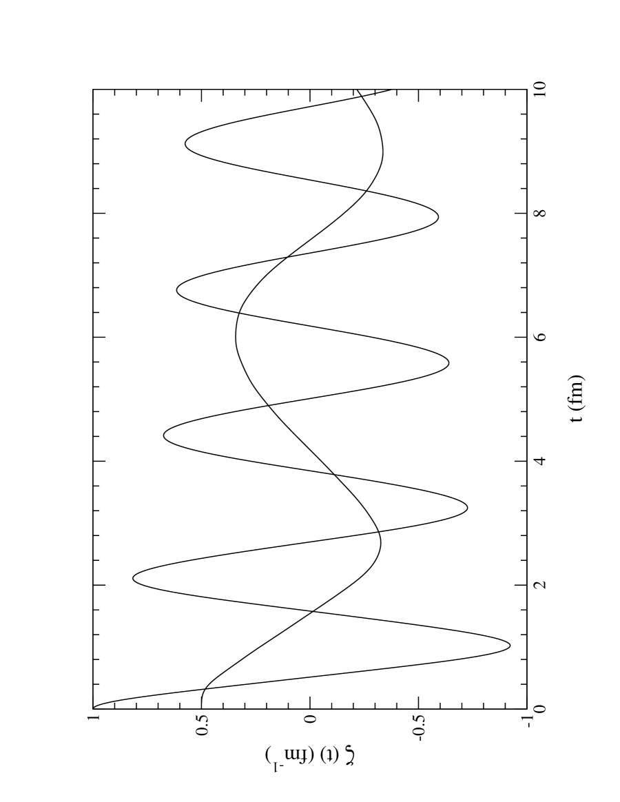
FIG. 1.:

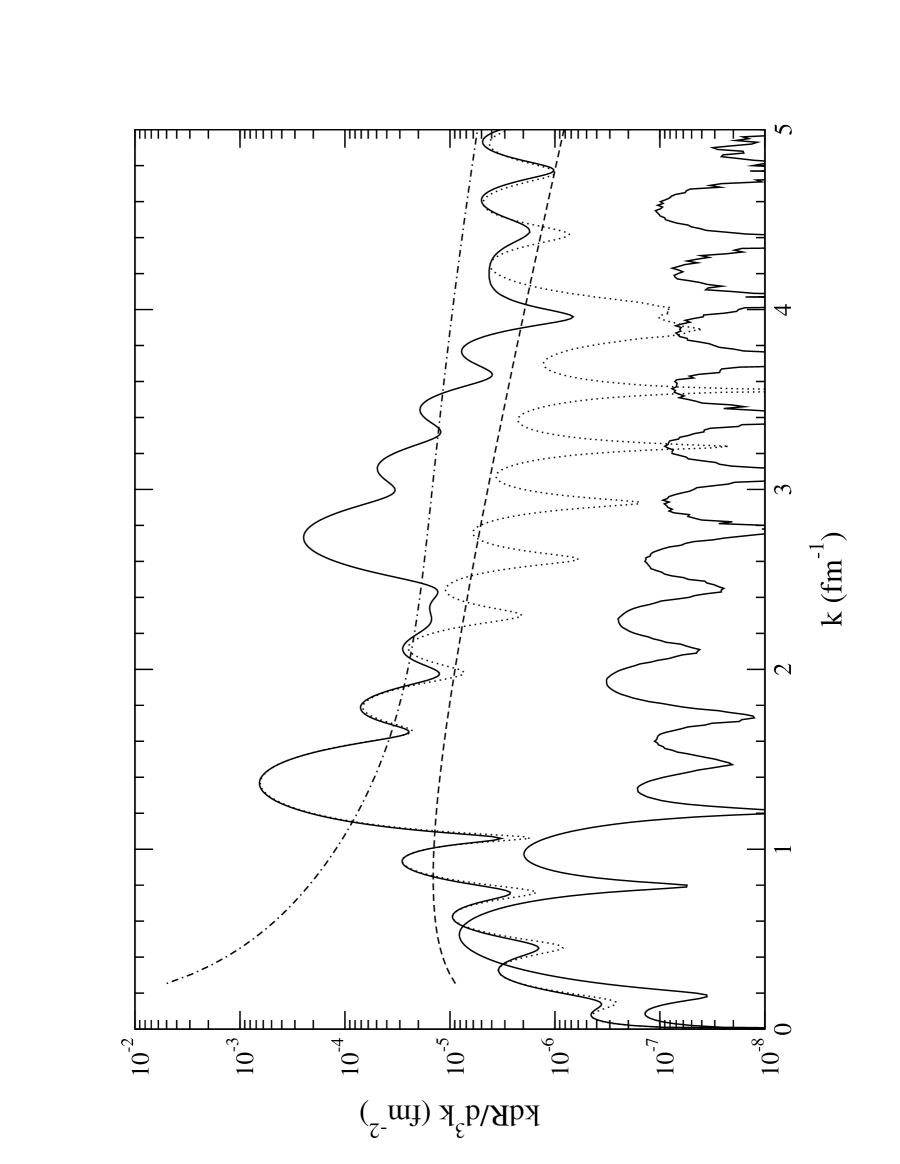
FIG. 2.:

REFERENCES

• [1] J. D. Bjorken, Int. J. Mod. Phys. A7, 4189 (1992); Acta Phys. Polon. B 23, 561 (1992); A. Anselm, Phys. Lett. B 217, 169 (1989); A. Anselm and M. Ryskin, Phys. Lett. B 226, 482 (1991); J. P. Blaizot and A. Krzywicki, Phys. Rev. D 46, 246 (1992); K. L. Kowalski and C. C. Taylor, CWRU report 92- hep-ph/9211282 (unpublished); J. D. Bjorken, K. L. Kowalski, and C. C. Taylor, Proceedings of Les Rencontres de Physique del Valle d’Aoste, La Thuile (SLAC PUB 6109) (1993); G. Amelino-Camelia, J. D. Bjorken, S. E. Larsson, Phys. Rev. D 56, 6942 (1997); J. D. Bjorken, Acta Phys. Polon. B 28, 2773 (1997).
• [2] K. Rajagopal and F. Wilczek, Nucl. Phys. B 399, 395 (1993); K. Rajagopal and F. Wilczek, Nucl. Phys. B 404, 577 (1993); for a review, see K. Rajagopal in “Quark-Gluon Plasma”, Ed. by R. C. Hwa (World Scientific, Singapore, 1995).
• [3] S. Gavin, A. Gocksch, and R. D. Pisarski, Phys. Rev. Lett, 72, 2143 (1994); S. Gavin and B. Muller, Phys. Lett. B 329, 486 (1994); Z. Huang and X.-N. Wang, Phys. Rev. D 49, 4335 (1994); J. Randrup, Phys. Rev. Lett 77, 1226 (1996); Phys. Rev. D 55, 1188 (1997); Nucl. Phys. A 616, 531 (1997).
• [4] F. Cooper, Y. Kluger, E. Mottola, and J. P. Paz. Phys. Rev. D 51, 2377 (1995); Y. Kluger, F. Cooper, E. Mottola, J. P. Paz, and A. Kovner, Nucl. Phys. A 590, 581 (1995); F. Cooper, Y. Kluger, and E. Mottola, Phys. Rev. C 54, 3298 (1996); M. A. Lampert, J. F. Dawson, and F. Cooper, Phys. Rev. D 54, 2213 (1996).
• [5] D. Boyanovsky, H. J. de Vega, and R. Holman, Phys. Rev. D 51, 734 (1995).
• [6] Z. Huang and X.-N. Wang, Phys. Lett. B 383, 457 (1996); Y. Kluger, V. Koch, J. Randrup, and X.-N. Wang, Phys. Rev. C 57, 280 (1998).
• [7] D. Boyanovsky, H. J. de Vega, R. Holman, and S. Prem Kumar, Phys. Rev. D 56, 5233 (1997).
• [8] D. Boyanovsky, H. J. de Vega, R. Holman, and S. Prem Kumar, Phys. Rev. D 56, 3929 (1997).
• [9] H. Minakata and B. Muller, Phys. Lett. B 377, 135 (1996).
• [10] R. Davidson, N. C. Mukhopadhyay and R. Wittman, Phys. Rev. D 43, 71 (1991).
• [11] D. Boyanovsky, H. J. de Vega, R. Holman, S. Prem Kumar, and R. D. Pisarski, Phys. Rev. D 58, 125009 (1998); S. Prem Kumar, D. Boyanovsky, H. J. de Vega, and R. Holman, Phys. Rev. D 61, 065002 (2000), and references therein.
• [12] D. Boyanovsky and H. J. de Vega, Phys. Rev. D 47, 2343 (1993); D. Boyanovsky, D.-S. Lee, and A. Singh, Phys. Rev. D 48, 800 (1993); D. Boyanovsky, H. J. de Vega and R. Holman, Phys. Rev. D 49, 2769 (1994); D. Boyanovsky, H. J. de Vega, R. Holman, D.-S. Lee, and A. Singh, Phys. Rev. D 51, 4419 (1995); D. Boyanovsky, M. D’Attanasio, H. J. de Vega, R. Holman, and D.-S. Lee, Phys. Rev. D 52, 6805 (1995); D. Boyanovsky, H. J. de Vega, D.-S. lee, Y. J. Ng, and S.-Y. Wang, Phys. Rev. D 59, 125009 (1999); S.-Y. Wang, D. Boyanovsky, H. J. de Vega, D.-S. Lee, and Y. J. Ng, Phys. Rev. D 61, 065004 (2000).
• [13] M. Le Bellac, Thermal Field Theory (Cambridge University Press, 1989).
• [14] N. MacLachlan, Theory and Application of Mathieu Functions (Dover, New York, 1961).
• [15] J. Kapusta, P. Lichard, and D. Seibert, Phys. Rev. D 44, 2774 (1991).
• [16] H. Nadeau, J. Kapusta, and P. Lichard, Phys. Rev. C 45, 3034 (1992); 47, 2426 (1993); L. Xiong, E. Shuryak, and G. E. Brown, Phys. Rev. D 46, 3798 (1992).