Three flavour neutrino oscillations in models with large extra dimensions

Abstract

The key challenges for models with large extra dimensions, posed by neutrino physics are: first to understand why neutrino masses are small and second, whether one can have a simultaneous explanation of all observed oscillation phenomena. There exist models that answer the first challenge by using singlet bulk neutrinos coupled to the standard model in the brane. Our goal in this paper is to see to what extent the simplest versions of these models can answer the second challenge. Our conclusion is that the minimal framework that has no new physics beyond the above simple picture cannot simultaneously explain solar, atmospheric and LSND data, whereas there are several ways that it can accommodate the first two. This would suggest that confirmation of LSND data would indicate the existence of new physics either in the brane or in extra dimensions or both, if indeed it turns out that there are large extra dimensions.
PACS: 14.60.Pq; 14.60.St; 11,10.Kk;

I Introduction

Particle physics models where there are large hidden space dimensions beyond the three familiar ones have been the focus of intense activity during the past two years[1, 2]. Beyond the simple reason that such extra dimensions are predicted by string theories, a major point of interest in these models is that often these large extra dimensions come with a TeV scale for the strings which leads to a plethora of new observable phenomena in collider as well in other arenas of particle physics and cosmology.

In order for these models to provide a satisfactory description of low energy particle physics, they must handle some obvious problems that come with the existence of a fundamental scale in the multi-TeV range. One such problem has to do with understanding the small neutrino masses in a natural manner. The conventional seesaw[3] explanation which is believed to provide the most satisfactory way to understand this, requires that the new physics scale (or the scale of $SU(2)_{R}\times U(1)_{B-L}$) be around $10^{12}$ GeV or higher. Clearly, low string scale theories do not have any fundamental scale of that type. Moreover, the low value of the string scale leads to enhanced (and unacceptable) contributions to neutrino masses from higher dimensional operators. While there are suggestions involving thick branes with point splitting[4] to remedy similar problems that arise from $\Delta B\neq 0$ operators, they don’t work for neutrino mass operators. Therefore, a necessary ingredient to understand small neutrino masses in the low string scale models is to assume that theory have a $B-L$ symmetry. This will forbid higher dimensional operators $LHLH/M^{*}$ ($M^{*}$ is the string scale), which are the source of the problem for neutrino masses.

Depending on whether $B-L$ is a global or local symmetry, one can have two ways to solve the neutrino mass problem in models with large extra dimensions. In the former case, discussed in [6], one has to introduce singlet bulk neutrinos which then lead to small Dirac masses for them. On the other hand, if $B-L$ symmetry is chosen to be a local symmetry, anomaly cancellation requires that, right handed neutrinos be present in the brane as in the models discussed in Ref.[7, 8]. Since local $B-L$ must be broken to avoid massless gauge bosons, one again has to deal with the induced operators of the same type as above with $M^{*}=M_{B-L}$. It was shown in Ref.[7, 8] that to get neutrino masses in the desired eV range, one must have string scale $M^{*}\simeq M_{B-L}\sim 10^{9}$ GeV range or higher. As a result, a class of experimentally accessible phenomenological predictions are lost, although long range gravity tests are still possible. These models are similar to the ones discussed in [9].

In the context of models that have global $U(1)_{B-L}$ symmetry, one can maintain the TeV scale for the strings and still get small neutrino masses by introducing isosinglet neutrinos in the bulk as has already been discussed in Ref.[6]. These models are interesting because a very minimal set of particles beyond the standard model are sufficient to get small neutrino masses. Key reason for this result is the relation between the fundamental scale, $M^{*}$, the radius of the extra dimensions, $R$, and effective Planck scale, $M_{P\ell}$,

$$M^{*2+n}R^{n}=M^{2}_{P\ell},$$ (1)

Since the singlet neutrino is a bulk field, the effective couplings of its Fourier modes to the standard model fields are naturally suppressed by the ratio $M^{*}/M_{P\ell}$, which for a TeV $M^{*}$ produces the right order of magnitude for neutrino masses.

An analysis of the implications of the mixing profile in these models for solar neutrino deficit was discussed in [10]. Also, implications for atmospheric neutrinos were discussed in [11], and some phenomenological bounds were given in [10, 11, 12, 13]. Our goal in this paper is to attempt a unified explanation of all known neutrino oscillation data i.e. solar, atmospheric as well as LSND under different assumptions for the initial input parameters for the minimal bulk neutrino scenario.

The basic reason for embarking on such an ambitious program is the encouraging feature that the masses of the lower KK modes of the bulk neutrinos are given by integral multiples of $R^{-1}$ which is of order $10^{-3}$ eV when $R\sim$ millimeter. This is of the right order necessary to solve the solar neutrino problem via small angle MSW mechanism using $\nu_{e}$ to $\nu_{s}$ oscillation. Thus we see that there exists a natural way to understand the lightness of the sterile neutrino[8, 10, 14], a situation if realized would pose a major challenge to four dimensional theories. Once the solar neutrino problem is understood, it would appear that all the necessary ingredients are at hand to understand the atmospheric and LSND data using oscillations among the familiar neutrinos i.e. $\nu_{e}\rightarrow\nu_{\mu}$ for LSND and $\nu_{\mu}\rightarrow\nu_{\tau}$ for atmospheric.

This program has already been undertaken in special parameter domains and it has already been suspected[8, 11] that it does not really work. Our goal is to extend these discussions to a somewhat larger parameter domain to see if there is chance for this program to succeed and unfortunately our answer is also in the negative. Our work complements the above works and extends them. Specifically, we try to give analytical reasonings to see how the different oscillation data can (or cannot) be understood. Since we do not take recourse to a detailed numerical analysis, we cannot rule out the possibility that some small parameter domain exists where all data can be accommodated; but we consider that unlikely.

The negative conclusion of our work, combined with the works of [8, 11] implies with virtual certainty that in the large extra dimension framework, understanding the neutrino data does require new physics beyond the standard model in the brane or new physics in extra dimensions or both.

Our basic strategy is as follows: we start by requiring that the parameters of the theory provide an explanation for solar and atmospheric oscillations. Then we ask whether they can account for the small LSND probability of $\nu_{e}$ appearance from the $\nu_{\mu}$ beam.

This paper is organized as follows: in section II, we discuss neutrino oscillations with a single flavour, which depends on two parameters, the bulk radius and a dimensionless parameter $\xi$ related to the Dirac mass term in the theory. The latter defines the pattern of neutrino oscillations. This analysis sets the stage for the three flavour case, which we discuss in section III for various possible domains of the parameter space. We end the paper with a concluding section that summarizes the results and discusses their implications.

II Oscillations with a single flavour

Let us begin our discussion by focusing on the simplest case with one generation of fermions in the brane and one bulk neutrino, to understand the general profile of the neutrino oscillations in models with large extra dimensions. We will discuss the necessary ingredients to understand the three flavour case that is explored in the next section. Obviously, the fields that could propagate in the extra dimensions are chosen to be gauge singlets. Let us denote bulk neutrino by $\nu_{B}(x^{\mu},y)$. It has a five dimensional kinetic energy term and a coupling to the brane field $L(x^{\mu})$ given by

$${\cal L}=\kappa\bar{L}H\nu_{BR}(x,y=0)+\int dy\ \bar{\nu}_{BL}(x,y)\partial_{5}\nu_{BR}(x,y)+h.c.$$ (2)

where from the five dimensional kinetic energy, we have only kept the 5th component that contributes to the mass terms of the KK modes in the brane; $H$ denotes the Higgs doublet, and $\kappa=h{M^{*}\over M_{P\ell}}$ the suppressed Yukawa coupling. It is worth pointing out that this suppression is independent of the number and radius hierarchy of the extra dimensions, provided that our bulk neutrino propagates in the whole bulk. For simplicity, we will assume that there is only one extra dimension with radius of compactification as large as a millimiter, and the rest with much smaller compactification radii. The smaller dimensions will only contribute to the relationship (1) but its KK excitations will be very heavy and decouple from neutrino spectrum. Thus, all the analysis could be done as in five dimensions.

The first term in Eq. (2) will be responsible for the neutrino mass once the Higgs field develops its vacuum. The induced Dirac mass parameter will be given by $m=\kappa v$, which for $M^{*}=1$ TeV is about $h\cdot 10^{-5}$ eV. Obviously this value depends only linearly on the fundamental scale. Larger values for $M^{*}$ will increase $m$ proportionally. After introducing the expansion of the bulk field in terms of the KK modes, the Dirac mass terms in (2) could be written as

$$(\bar{\nu}_{eL}\bar{\nu}^{\prime}_{BL})\left(\begin{array}[]{cc}m&\sqrt{2}m\\ 0&\partial_{5}\end{array}\right)\left(\begin{array}[]{c}\nu_{0B}\\ \nu^{\prime}_{BR}\end{array}\right),$$ (3)

where our notation is as follows: $\nu^{\prime}_{B}$ represents the KK excitations, the off diagonal term $\sqrt{2}m$ is actually an infinite row vector of the form $\sqrt{2}m(1,1,\cdots)$. The operator $\partial_{5}$ stands for the diagonal and infinite KK mass matrix whose $n$-th entrance is given by $n/R$. This notation was introduced in [7] to represent the infinite mass matrix in a compact manner.

Using this short hand notation makes it easier to calculate the exact eigenvalues and the eigenstates of this mass matrix [8]. Simple algebra yields the characteristic equation

$$2\lambda_{n}=\pi\xi^{2}\cot(\pi\lambda_{n}),$$ (4)

with $\lambda_{n}=m_{n}R$, $\xi=\sqrt{2}mR$, and where $m_{n}$ is the mass eigenvalue [6, 10]. The eigenstates, on the other hand are given symbolically by [8]

$$\tilde{\nu}_{nL}={1\over N_{n}}\left[\nu_{L}+{\sqrt{2}m\partial_{5}\over m_{n}^{2}-\partial_{5}^{2}}\,\nu^{\prime}_{BL}\right],$$ (5)

where the sum over the KK modes in the last term is implicit. $N_{n}$ is the normalization factor given by

$$N^{2}_{n}={1\over\xi^{2}}\left(\lambda_{n}^{2}+f(\xi)\right),$$ (6)

where $f(\xi)=\xi^{2}/2+\pi^{2}\xi^{4}/4$. Figures 1 and 2 depict the exact numerical results of $\lambda_{n}$ and $N_{n}$ for several choices for the value of the $\xi$ parameter. Using the expression (5), we can write down the weak eigenstate $\nu_{L}$ in terms of the massive modes as

$$\nu_{L}=\sum_{n=0}^{\infty}{1\over N_{n}}\tilde{\nu}_{nL}.$$ (7)

Thus, the weak eigenstate is actually a coherent superposition of an infinite number of massive modes. Therefore, even for this single flavour case, the time evolution of the mass eigenstates involves in principle all mass eigenstates and is very different from the simple oscillatory behaviour familiar from the conventional two or three neutrino case. The time dependent survival probability is given by

$$P_{surv}(L) = \left|\langle\nu_{L}(L)|\nu_{L}(0)\rangle\right|^{2}=\left|\sum_{n=0}^{\infty}{e^{i{L\over 2ER^{2}}\lambda_{n}^{2}}\over N^{2}_{n}}\right|^{2}=1-2\sum_{k,n=0}^{\infty}{\sin^{2}\left({L\over 4ER^{2}}(\lambda_{n}^{2}-\lambda_{k}^{2})\right)\over N_{n}^{2}N_{k}^{2}}.$$ (8)

It is clear that the survival probability depends strongly on the parameter $\xi$, reflecting the universal coupling of all the KK components of $\nu_{B}$ with $\nu_{L}$ in (2). Figures 3 and 4 show the profile of the survival probability obtained from the numerical solutions for three different values of $\xi$ and is clearly very different from simple familiar oscillatory behaviour. However, to better understand these results, we will follow an analytical approach in what follows.

It is simpler to consider the two limiting cases. First let us assume that $\xi\ll 1$. As already known [8, 10], the eigenvalues in this case are given by $\lambda_{0}=mR$, and $\lambda_{n}=n$ otherwise. Therefore, to a good approximation, we may take the mixing parameters $N_{0}=\eta$, and $N_{n}=(n/\xi)\eta$ for non zero $n$. Where the extra factor $\eta=(1+\pi^{2}\xi^{2}/6)^{1/2}$ is introduced to keep the proper normalization in the expansion (7). This approximation is confirmed by our figures 1 and 2. The survival probability is now given as

$$P_{surv}(L)=1-{4\over\eta^{4}}\xi^{2}\sum_{n=1}^{\infty}{\sin^{2}\left({n^{2}L\over 4ER^{2}}\right)\over n^{2}}-{2\over\eta^{4}}\xi^{4}\sum_{k,n=1}^{\infty}{\sin^{2}\left[{(n^{2}-k^{2})L\over 4ER^{2}}\right]\over n^{2}k^{2}}.$$ (9)

It is simple to see from last expression that the probability has an oscillation length $L_{osc}=4\pi ER^{2}$. A typical profile in this case is depicted in figure 4. Also, the main contribution to the oscillation pattern comes from the lowest elements of the tower, which turns out to be the main component of $\nu_{L}$. Another way to see this result is to note that $\xi$ could be made small by making $R$ small; but this makes the KK excitation masses large so that they decouple from the light sector of the theory leaving only the right handed component of the zero mode of the bulk neutrino, $\nu_{BR}$ to form a Dirac mass with $\nu_{L}$ and stay light. The left-handed zero mode decouples and remains massless.

In the $\xi\ll 1$ limit, the small mixing with the tower elements leads to an oscillation pattern dominated by the lightest KK mode with a mass just about $1/R$ and more or less simulate the familiar oscillatory one. This can happen, for instance, if $R\sim 0.2\ mm$, which gives $1/R^{2}\sim 10^{-6}~{}eV^{2}$, just about what it is needed to provide an explanation to the solar neutrino problem assuming a small MSW mixing angle [10]. To use this case to compare with solar neutrino data, one needs to include the matter effect, which has already been discussed in Ref.[10] and we do not enter into this here.

A more direct application of the formula in Eq. (9) can be made to discuss the atmospheric neutrino oscillations, which is a vacuum oscillation. However, to get the equivalent of large mixing angle we need to adjust $\xi\sim 1$ and $1/R^{2}\sim\Delta m^{2}_{atm}$, which means that Eq. (9) is not applicable and we must therefore use Eq. (8) and study its large $\xi$ limit.

To discuss this, we start with the limit when $\xi\gg 1$. First thing to note is that the pattern of eigenvalues is very different in this case from the small $\xi$ case. For small values of $n$ the eigenvalues are well approximated by $\lambda_{n}={2n+1\over 2}$, while $N_{n}$ becomes $n$ independent until certain cut off value that roughly speaking is given by $n_{\Lambda}=\pi^{2}\xi^{2}/4$. Beyond that point $\lambda_{n}\approx n$ and we may no longer neglect the contribution of $\lambda_{n}$ to (6). This results in a suppression of $N_{n}$ that goes like $1/n$. It should therefore be reasonable to consider as a first approximation that the expansion (7) is cut off at $n_{\Lambda}$, and that all the mass eigenstates contributing to $\nu_{L}$ are equally suppressed by $1/\sqrt{n_{\Lambda}}$. In this approximation, we obtain the survival probability to be

$$P_{surv}(L)=1-{2\over{n_{\Lambda}}^{2}}\sum_{k,n=0}^{n_{\Lambda}}\sin^{2}\left[{L\over 4ER^{2}}(\lambda_{n}^{2}-\lambda_{k}^{2})\right].$$ (10)

Certainly, this relation presents a oscillatory profile, however, the superposition of the equally suppressed oscillations will result most of the time on a destructive interference, with the exception of the very sharp resonances that appear each time $L$ reaches a multiple of the oscillation length. In other words, $\nu_{L}$ is a superposition of a large number of mass eigenstates, with masses covering a large range, from $1/2$ to $n_{\Lambda}$ in units of $1/R$, all of them contributing by the same amount. As a result, once $\nu_{L}$ is released, one may surmise that the time evolution of the different components will most likely wash out the original coherent superposition and the initial $\nu_{L}$ will almost disappear. As fig. 3 shows, this conclusion is borne out by the the numerical analysis. To get an analytical result that also supports this conclusion, note that in the sum in Eq. (10), the dominant contributions come when $n\neq k$ in which case each term in the sum averages to $1/2$ and on performing the double sum it is easy to see that one arrives at $\bar{P}_{surv}\approx 1/{n_{\Lambda}}$.

If $n_{\Lambda}$ is very large, it suppresses the survival probability too much and cannot help in the understanding of the atmospheric data. So, clearly, if we wanted an understanding of the atmospheric data, we must assume smaller $\xi$, perhaps values closer to one. In this case, truncating the sum in the expression for the survival probability in Eq. (9), cannot be justified and we must seek an alternative way to deal with Eq. (8). An approach suggested in [11] is to use a continuous approximation to the sum in Eq. (8), which leads to

$$P_{surv}(z)=\left|\int_{0}^{\infty}\!dn{e^{izn^{2}}\over n^{2}+f(\xi)}\right|^{2}\xi^{4}=\left({\pi^{2}\xi^{4}\over 4f(\xi)}\right)\left|1-{\rm erf}\left(\sqrt{izf(\xi)}\right)\right|^{2},$$ (11)

where $z=L/2ER^{2}$. Clearly, for large $\xi$; $f(\xi)\sim\pi^{2}\xi^{4}/4$, and last expression in Eq. (11) simplifies. In order to study the dependence of $P_{surv}(z)$ on $\xi$, we plot $P_{surv}$ in Fig. 3 in the continuous and discrete approximations. One thing that emerges is the non-oscillatory nature of the function as we exceed $\xi=1$. We also see that the continuous limit gives a good approximation for the slope (see figure 3), even for cases where $\xi\leq 1$ [11]. This expression, however, does not represent the survival probability in the limit $\xi\ll 1$, since in this case (i.e. $\xi\ll 1$), the $P_{surv}$ has an oscillatory behaviour unlike the last term in Eq. (11) (see figure 4). In the overlap region close to $\xi\simeq 1$, one may evaluate the second term in Eq. (11) in a slightly different way which leads to an expression for the survival probability as

$$P_{surv}(\zeta)=\rho^{2}(\zeta)+\vartheta^{2}(\zeta),$$ (12)

where we have introduced the new variable $\zeta=\sqrt{zf(\xi)}=(\pi\xi^{2}/2R)\sqrt{L/2E}$ and the functions $\rho(\zeta)=1-C(\zeta)-S(\zeta)$; and $\vartheta(\zeta)=C(\zeta)-S(\zeta)$ with $S$ and $C$ the sine and cosine Fresnel integrals:

$\displaystyle C(\zeta)=\sqrt{2\over\pi}\int_{0}^{\zeta}\!dt~{}\cos(t^{2})\qquad\mbox{ and }\qquad S(\zeta)=\sqrt{2\over\pi}\int_{0}^{\zeta}\!dt~{}\sin(t^{2}).$We draw attention to the fact that $\zeta$ involves not only the model parameters $\xi$ and $R$ but also the experimental variable $z$. Thus for a given model, the variable $\zeta$ has different values for different oscillation experiments; for instance, for the atmospheric neutrino case, a typical value for $\zeta\sim\frac{\pi\xi^{2}}{2R}1.2\times 10^{2}$ eV^-1.

The expression (12) is valid just before $P_{surv}(\zeta)$ reaches the average, $\bar{P}_{surv}=4/\pi^{2}\xi^{2}$. In figure 5 we present the behaviour of $\rho$, $\vartheta$ and $P_{surv}$. Note the steep fall off of $P_{surv}$ as $\zeta$ increases. For $\zeta=1$, $P_{surv}$ has already dropped under 20%, which is smaller than the observed deficit in solar and atmospheric data. Therefore, if we want to fit the overall suppression of the atmospheric neutrinos, we must remain in a very narrow range of parameters. A rough estimate of these parameters may be obtained by expanding (12) to first order on $\zeta$, which yields

$$P_{surv}(\zeta)\approx 1-2\sqrt{2\over\pi}\zeta=1-2\sqrt{\pi}\left({\xi^{2}\over R}\right)\left({L\over 4E}\right)^{1\over 2}.$$ (13)

Now, we may invert the last equation to get

$${\xi^{2}\over R}\simeq{(1-\bar{P}_{exp})\over\sqrt{4\pi}}\left({L\over 4E}\right)^{-{1\over 2}}_{exp}.$$ (14)

Using average values for the $L,E$ and $P_{exp}$ for atmospheric neutrinos, we find $\xi^{2}/R\approx 10^{-2}eV$. Note that this naive approximation gives just about the value obtained by the numerical fitting of the data in [11]. For this value, as $\xi>1$, we get $R$ in the range $10^{-3}~{}eV<1/R<10^{-2}~{}eV$ implying $1<\xi^{2}<10$. Thus a solution to the atmospheric neutrino puzzle using KK modes requires that $R$ be in the sub-millimeter range. This in turn determines how large $M^{*}$ should be to avoid any unwanted large fine tuning. We see that for $m\geq 10^{-3}~{}eV$ and Yukawa coupling $h$ of order one, we need $M^{*}\geq 100~{}TeV$.

We also point out that in the case of $\xi\geq 1$, extra dimensions must be much larger than a millimeter if we want to fit the solar neutrino data either via MSW or via vacuum oscillation. To see this note that if we take $\Delta m^{2}_{sol}\sim 10^{-6}$ eV², this would imply $L/4E\sim 1/\Delta m^{2}_{sol}\sim 10^{6}$ eV^-2. Putting this in Eq. (13), we get $\xi^{2}/R\simeq 10^{-4}$ eV. For $\xi\gg 1$, this implies that $R\gg 0.2$ mm. Similar estimate for the case of vacuum oscillation yields $R\gg 2$ cm. Therefore, in all our discussion of solar neutrino oscillations involving the bulk neutrinos, we will work in the approximation $\xi\ll 1$.

Let us now summarize our findings for a single neutrino case: for $\xi\ll 1$, $P_{surv}$ has an oscillatory behaviour as given by (9). As $\xi$ approaches 1, $\lambda_{n}$ starts to deviate from the integer value $n$, which in turn disturbs the periodic nature of $P_{surv}$ and the maximum and minimum values of probability are not reached away from the source [6]. This picture gets worse as one approaches $\xi\gg 1$ when a very sharp slope drives the probability near zero as we move away from the source of the neutrinos and it remains around its average, $4/\pi^{2}\xi^{2}$, most of the time. For this reason, whenever we try to fit the atmospheric neutrino data with bulk neutrinos, the value of $\xi$ must be tuned to a very narrow range.

Let us apply the discussions of this section to study how the oscillation of known neutrinos to bulk ones would effect the current experiments such as CHOOZ-PALOVERDE, LSND and the atmospheric neutrinos. For this purpose, we first note that in contrast with the usual two neutrino oscillation case, where the pattern is determined by three parameters, the mixing angle $\theta$, the $\Delta m^{2}$ and $L/4E$ for the experiment, in the case of bulk neutrino oscillation, we have $L/4E$ characterizing an experiment like before, bulk radius $R$, which replaces $\Delta m^{2}$ (which we will assume to be in the milli-meter range) and model parameter $\xi$ (which is the analog of the mixing angle). For a given $R$, $\xi$ is the only parameter characterizing the oscillation pattern. In Fig. 6, we plot the variation of the survival probability $P_{surv}$ against $\xi$ for the various cases mentioned above for a typical characteristic value of $L/4E$. We see from this figure that to explain the observed overall deficit of atmospheric neutrinos by nearly 50%, one needs to go to $\xi\sim 1.5$ or so. This conclusion is in acoord with our conclusion based on Eq. (14) above.

III Three flavour oscillations

Let us now apply the discussion of the previous section to the case of three standard model generations in the brane so that we have three brane neutrinos $\nu_{e,\mu,\tau}$. To give masses to all of them in a minimal scenario, we will use three bulk neutrinos and allow arbitrary Yukawa couplings between the bulk and the brane neutrinos. This leads to an arbitrary Dirac mass matrix that involves the familiar left-handed neutrinos and the right handed Kaluza-Klein modes of the bulk neutrinos. As already discussed in [8], the most general Dirac mass terms with three flavours may be written, after a rotation of the bulk fields, as

$${\cal L}=\bar{\bf\nu}_{L}\cdot UM_{D}\cdot{\bf\nu}_{BR}(y=0)+\int dy\,\bar{\bf\nu}_{BL}\cdot\partial_{5}\cdot{\bf\nu}_{BR}+h.c.,$$ (15)

where $U$ is a unitary matrix and $M_{D}=Diag(m_{1},m_{2},m_{3})$, in the basis where ${\bf\nu}_{L}=(\nu_{e},\nu_{\mu},\nu_{\tau})_{L}$; and ${\bf\nu}_{B}=(\nu^{1}_{B},\nu^{2}_{B},\nu^{3}_{B})$. The mass parameters $m_{\alpha}$ are just the eigenvalues of the Yukawa coupling matrix multiplied by $v$, the vacuum expectation value of the standard model doublet field. They are of the order of eV or less since the couplings of the bulk modes to the brane fields are naturally suppressed, as already stated on the previous section.

Now, to simplify the discussion, we rotate the weak eigenstate neutrinos $\nu_{a}$ to the ones related to the weak eigenstates by the rotation $U$ i.e. $\nu_{a}=U_{a\alpha}\nu_{\alpha}$, where $a=e,\mu,\tau$ and $\alpha=1,2,3$. We then have

$${\cal L}=\sum_{\alpha=1}^{3}\left[m_{\alpha}\bar{\nu}_{\alpha L}\nu^{\alpha}_{BR}(y=0)+\int dy\,\bar{\nu}^{\alpha}_{BL}\partial_{5}\nu^{\alpha}_{BR}+h.c.\right].$$ (16)

This reduces the problem to a consideration of three KK towers mixing with three neutrinos which are related to the weak interaction eigenstates by the unitary matrix $U$ defined above. Each tower is characterized by its $\xi_{\alpha}$ parameter defined in analogy with section II as $\xi_{\alpha}\equiv\sqrt{2}m_{\alpha}R$. After diagonalization of the mass matrices in each tower, each standard neutrino can be written as a coherent superposition of the three different towers of mass eigenstates:

$$\nu_{a}=\sum_{\alpha=1}^{3}U_{a\alpha}\nu_{\alpha}=\sum_{\alpha=1}^{3}\sum_{k=0}^{\infty}U_{a\alpha}{1\over N_{\alpha k}}\tilde{\nu}_{\alpha k}.$$ (17)

This expression generalizes Eq. (7). It is now clear that the three flavour oscillations will correspond to the oscillations among the three towers. In this regards, the explanation to neutrino puzzles is not any more described in terms of three single neutrinos, as in the usual case; instead all the KK modes can contribute (unless all the KK excitations decouple from the spectrum).

To proceed further, let us define the partial transition probabilities

$$p_{\alpha\beta}(L)\equiv\overline{\langle\nu_{\alpha}(L)|\nu_{\alpha}(0)\rangle}\langle\nu_{\beta}(L)|\nu_{\beta}(0)\rangle.$$ (18)

Notice that the diagonal component $p_{\alpha\alpha}$ may be interpreted as the survival probability of $\nu_{\alpha}$, and it takes the form of Eqs. (9) and (12) in that case. It of course involves the $\nu_{\alpha}$’s and not the flavor eigenstates as is obvious. The transition probability among standard flavours can be written in terms of the $p_{\alpha\beta}$’s as

$$P_{ab}=\sum_{\alpha\beta}U^{*}_{a\alpha}U_{b\alpha}U^{*}_{b\beta}U_{a\beta}\ p_{\alpha\beta}.$$ (19)

Neglecting all CP phases we may expand Eq. (18) to the form

$$p_{\alpha\beta}=1-2\sum_{k,n=0}^{\infty}{\sin^{2}\left(\frac{z}{2}(\lambda_{\alpha n}^{2}-\lambda_{\beta k}^{2})\right)\over{N^{2}_{\alpha n}(\xi_{\alpha})N^{2}_{\beta k}(\xi_{\beta})}}.$$ (20)

Now, we are ready to address the oscillation problem. Our approach will be as follows: we will first select the parameter range that provides overall reduction required to explain the solar and atmospheric data, and then ask whether for the same range of parameters we can explain the observed oscillation between $\bar{\nu}_{\mu}$ to $\bar{\nu}_{e}$ reported by LSND. Without loss of generality, we can assume the hierarchy $\xi_{1}<\xi_{2}<\xi_{3}$. We consider three possible scenarios:

• $\xi_{1,2,3}\ll 1$;

• $\xi_{1,2}\ll 1\leq\xi_{3}$ and

• $\xi_{1}\ll 1\leq\xi_{2,3}$.

The case where all $\xi_{a}>1$ is already ruled out since, as we discussed earlier, it cannot explain the solar neutrino data without implying that the extra dimensions be too large. We therefore do not discuss this case. In the discussion of our results, the following expressions for the partial transition probabilities will be very useful: If $\xi_{\alpha,\beta}\ll 1$, then

$$p_{\alpha\beta}={1\over\eta_{\alpha}^{2}\eta_{\beta}^{2}}\left[\cos\left({L\over 2E}\Delta m_{\alpha\beta}^{2}\right)+\left(\xi_{\alpha}^{2}+\xi_{\beta}^{2}\right)c(z)+\xi_{\alpha}^{2}\xi_{\beta}^{2}\left(c^{2}(z)+s^{2}(z)\right)\right],$$ (21)

with $\Delta m_{\alpha\beta}^{2}=m_{\alpha}^{2}-m_{\beta}^{2}$; $\eta_{\alpha}^{2}=1+\pi^{2}\xi_{\alpha}^{2}/6$ and $z=L/2ER^{2}$ as before, and where we have introduced the functions

$$\left(\begin{array}[]{c}c(z)\\ s(z)\end{array}\right)=\sum_{n=1}^{\infty}{1\over n^{2}}\left(\begin{array}[]{c}\cos(zn^{2})\\ \sin(zn^{2})\end{array}\right).$$ (22)

It is simple to check that the diagonal term of Eq. (21) reduces to Eq. (9). For $\xi_{\alpha}\ll 1<\xi_{\beta}$ we get

$$p_{\alpha\beta}={1\over\eta_{\alpha}^{2}}c_{\beta}(z)+{\xi_{\alpha}^{2}\over\eta_{\alpha}^{2}}\left(c(z)\ c_{\beta}(z)+s(z)\ s_{\beta}(z)\right);$$ (23)

where we now used $c_{\beta}(z)=\cos(\zeta_{\beta}^{2})\rho(\zeta_{\beta})-\sin(\zeta_{\beta}^{2})\vartheta(\zeta_{\beta})$ and $s_{\beta}(z)=\sin(\zeta_{\beta}^{2})\rho(\zeta_{\beta})+\cos(\zeta_{\beta}^{2})\vartheta(\zeta_{\beta})$ with $\zeta_{\beta}=\sqrt{z}\pi\xi_{\beta}^{2}/2$, and $\rho$ and $\vartheta$ as defined in the previous section, we should stress that all those functions have a similar deep behaviour. And, finally, for $\xi_{\alpha,\beta}>1$ we have

$$p_{\alpha\beta}=c_{\alpha}(z)\ c_{\beta}(z)+s_{\alpha}(z)\ s_{\beta}(z).$$ (24)

Again, it is straightforward to check that the diagonal component of this equation reduces to Eq.(12).

A Case I: $\xi_{\alpha}\ll 1$

Substituting Eq. (21) into (19), we get, to leading order in $\xi_{\alpha}$

$$P_{ab}=\delta_{ab}-2\sum_{\alpha,\beta}U_{a\alpha}U_{b\alpha}U_{b\beta}U_{a\beta}\sin^{2}\left({L\over 4E}\Delta m_{\alpha\beta}^{2}\right)+O(\xi_{\alpha}^{2}).$$ (25)

Therefore, as expected, to this order, we obtain the standard expression for the transition probability well known for the three neutrino case. It is clear that in this scenario, solar and atmospheric data can be explained as in the usual three flavour neutrino models by adjusting the spacing of the different $\xi_{\alpha}$’s. For the solar neutrino puzzle, one may either use MSW or VO solution depending on how much fine tuning one is willing to tolerate.

For intermediate values where ${L/4E}\ll 1/\Delta m_{\alpha\beta}^{2}$, the leading corrections in $\xi$ become important. Expanding $P_{ab}$ up to order $\xi^{4}$, by introducing Eq. (21) and neglecting the standard oscillatory term we found

$$P_{ab} \approx \delta_{ab}\left[1-2\sum_{\alpha}|U_{a\alpha}|^{2}{\xi_{\alpha}^{2}\over\eta^{2}_{\alpha}}\left({\pi^{2}\over 6}-c(z)\right)\right]+\left(\sum_{\alpha}U_{a\alpha}U_{b\alpha}{\xi_{\alpha}^{2}}\right)^{2}I(z);$$ (26)

where we have denoted

$$I(z)=\left[{\pi^{4}\over 36}+c^{2}(z)+s^{2}(z)-{\pi^{2}\over 3}c(z)\right],$$ (27)

Notice that the first term between parenthesis on Eq. (26) contains the lower order correction to the standard survival probability in Eq. (25), while the second term, of oder $\xi^{4}_{\alpha}$ will be only relevant for flavour transitions. Taking the average on the last equations, and using that $\bar{c}=0$ and $\overline{c^{2}+s^{2}}=\pi^{4}/90$, we get

$$\bar{P}_{ab}\approx\delta_{ab}\left(1-\frac{\pi^{2}}{3}\sum_{\alpha}|U_{a\alpha}|^{2}{\xi_{\alpha}^{2}\over\eta^{2}_{\alpha}}\right)+{7\over 180}\pi^{4}\left(\sum_{\alpha}U_{a\alpha}U_{b\alpha}{\xi_{\alpha}^{2}}\right)^{2}.$$ (28)

This last expression generalizes that presented in Ref. [11], where only the contribution of $\xi_{3}$ was assumed.

It is clear that understanding LSND results in this case would require that $\nu_{\mu}$ first undergo a transition to the lower KK modes of the bulk neutrinos and then back to the $\nu_{e}$. One might hope that if we adjusted the extra dimension radius to be small enough $R^{-1}\sim 0.2-2$ eV, then one would get the right mass difference to fit LSND data. The key question then is to see whether the transition rate comes out right. For this purpose, we consider up to the lowest non-vanishing order in $\xi_{\alpha}$ for $P_{\mu e}$ given in (26), which after using the unitarity of $U$ and the fact that $\xi^{2}_{3}-\xi^{2}_{1}=2\Delta m_{atm}^{2}R^{2}$ turns out to have the form

$$P_{\mu e}\approx\sin^{2}2\theta_{\mu e}\ \left(\Delta m_{atm}^{2}R^{2}\right)^{2}I(z)$$ (29)

with $\sin^{2}2\theta_{\mu e}\equiv 4(U_{\mu 3}U_{e3})^{2}$. It is straightforward to check that $P_{\mu e}(L=0)=0$ by using the identities $c(0)=\pi^{2}/6$ and $s(0)=0$. From the limits obtained by the CHOOZ and Palo Verde collaboration, we know that $|U_{e3}|^{2}<0.03$ [15], and assuming $|U_{\mu 3}|^{2}=0.5$ for maximal mixing, the largest optimistic value for the mixing angle we may take is about $\sin^{2}2\theta_{\mu e}=0.06$. By fixing $L/E$ as for LSND, $I(z)$ becomes only a function of $R$ (since $z=L/2ER^{2}$). In figure 7 we have plotted $I(R)$ versus $R$. From this figure we see that for a reasonable large $R$ ($\sim 10~{}eV^{-1}$), the function $I(R)$ has very small values already. The combined effect with the factor $\Delta m_{atm}^{2}R^{2}<1$ will reduce $P_{\mu e}$ even more. Clearly, $P_{\mu e}$ will be maximal for the larger possible value of $R$. However, the largest allowed radius that permit us to still be confident in our approach is about $1/R\sim\sqrt{\Delta m_{atm}^{2}}\sim 0.06~{}eV$. A numerical calculation with these inputs gives for LSND $P_{\mu e}=3\times 10^{-4}$, which is one order of magnitude smaller than the observed anomaly in the $\bar{\nu}$ beam of LSND. Since higher order corrections in $\xi_{\alpha}$ to the probability are unlikely to introduce enough enhancement (a factor of 10 is needed), we conclude that this scenario yields a too small probability for $\nu_{\mu}-\nu_{e}$ transition to explain the LSND observations.

B Case II: $\xi_{1,2}\ll 1\leq\xi_{3}$

To proceed with this case, it is convenient to write the survival probability $P_{aa}$ in the following form:

$$P_{aa}=\sum_{\alpha,\beta=1,2}\left(U_{a\alpha}U_{a\beta}\right)^{2}\ p_{\alpha\beta}+2U_{a3}^{2}\sum_{\alpha=1,2}U_{a\alpha}^{2}\ p_{\alpha 3}+U_{a3}^{4}\ p_{33}.$$ (30)

The first term in the above equation can be written to leading order in the small $\xi$’s as follows:

$$\sum_{\alpha,\beta=1,2}\left(U_{a\alpha}U_{a\beta}\right)^{2}p_{\alpha\beta}\approx\left(1-U_{a3}^{2}\right)^{2}-\sin^{2}2\theta_{aa}\sin^{2}\left({L\over 4E}\Delta m_{21}^{2}\right)~{}+~{}O(\xi^{2})$$ (31)

where $\sin^{2}2\theta_{aa}=4(U_{a1}U_{a2})^{2}$. This term by itself can explain the solar neutrino deficit. Clearly, the standard two neutrino oscillation expression is recovered to this order if we set $U_{e3}\sim 0$ to satisfy the bounds imposed by the reactor data[15]. This will make the contributions of the last two terms in the survival probability (30) negligible and the first oscillatory term can then be used to solve the solar neutrino puzzle. One can of course use the MSW mechanism to solve the solar neutrino problem or the vacuum oscillation. The constraint on the parameter space is that the $\Delta m^{2}_{12}$ be appropriately adjusted. This does not impose any condition on the bulk radius and can be satisfied by the initial choice of parameters (the Yukawa couplings) in the theory. For instance, $M^{*}\sim 10$ TeV can lead to the MSW-type mass differences. Let us note that, if $\Delta m^{2}_{12}\sim 10^{-5}$ eV², then, we will have $|\xi^{2}_{1}-\xi^{2}_{2}|\sim 10^{-5}R^{2}$ (eV cm)².

Now let us consider $P_{\mu\mu}$. From Eq (30), we see that there are several contributions to the atmospheric neutrino deficit. First, there is the contribution of the towers labeled by $\xi_{1,2}$, which is oscillatory, although it can not be identified as in the usual $\nu_{\mu}\rightarrow\nu_{\tau}$ oscillations. Then, there is also the contribution induced by the term $p_{33}$ which is of the form of (12). Finally, there is also a mixed term, $p_{\alpha 3}$.

To proceed with the full discussion, let us consider two cases:

Case (i): $U_{\mu 3}=0$

If $U_{\mu 3}=0$, the last two contributions are removed and we get the survival probability

$$P_{\mu\mu}\approx 1-4\left(2U_{\mu 2}^{2}\Delta m_{21}^{2}R^{2}+\xi^{2}_{1}\right)\left(\frac{\pi^{2}}{6}-c(z)\right)$$ (32)

One might then hope that the oscillations into the lower KK modes with mass differences of about $1/R$ will do the job provided we choose $1/R\sim\sqrt{\Delta m_{atm}^{2}}$ to match the data. In this case, the atmospheric muon neutrinos oscillate into the sterile neutrinos, a possibility which has its characteristic tests. For this solution to work, one needs to assume $\xi_{1}\sim 1$ so that one gets maximal mixing. This in turn means that, to explain both solar and atmospheric neutrino data, an almost degeneracy $\xi_{1}\sim\xi_{2}$ must be maintained. This alters our explanation of the solar neutrino deficit since, now, these new contribution to it (see the $O(\xi^{2})$ terms in Eq. (28)), become more and more important and in fact of order one, making it hard to understand the solar neutrino deficit, since $c(z)\sim 1$. We will, therefore, consider this case as an unfavorable one for understanding the neutrino puzzles.

Case (ii): $U_{\mu 3}\neq 0$

Turning to the case where $U_{\mu 3}\neq 0$, if we keep $\xi_{1,2}\ll 1$ (to maintain our understanding of the solar neutrino data) then, the corrections of order $\xi^{2}_{1,2}$ to the transition probability become almost negligible and the dominant contribution to $P_{ab}$ then must come from $\xi_{3}$ corrections. This yields

$$P_{ab} \approx \left(\delta_{ab}-U_{a3}U_{b3}\right)^{2}-4(U_{a1}U_{b2})^{2}\sin^{2}\left({L\over 4E}\Delta m_{21}^{2}\right)$$ (34)

$$+2U_{a3}U_{b3}\left(\delta_{ab}-U_{a3}U_{b3}\right)c_{3}(z)+(U_{a3}U_{b3})^{2}p_{33}.$$

Notice that $p_{33}$ in the last equation has the same form as Eq. (12), and the function $c_{3}$ is the one defined above with the same sharp behaviour as $p_{33}$. Then specializing Eq. (34) to the $\nu_{\mu}$ in the atmospheric case, we get

$$P_{\mu\mu}\approx\left(1-U_{\mu 3}^{2}\right)^{2}+2U_{\mu 3}^{2}(1-U_{\mu 3}^{2})\ c_{3}(z)+U_{\mu 3}^{4}\ p_{33}.$$ (35)

From our naive analysis in the previous section we may expect that this equation can account for the atmospheric data without too much trouble as long as $\xi_{3}^{2}/R\sim 10^{-2}$ eV or so to make the width of the slope larger than the experimental parameters and to avoid the over washing of the $\nu_{\mu}$ flux. Indeed, it has been checked numerically in reference [11] that the atmospheric neutrino data can be fitted in this case if $U_{\mu 3}^{2}\approx 0.4$ and $\xi_{3}^{2}/R\sim 0.02~{}eV$. It is worth mentioning that a mixed explanation could be also possible, where the three towers contribute equally to provide atmospheric oscillations, but we will not discuss this case here.

An important point to note however is that due to the features of the function $c_{3}(z)$, the atmospheric neutrino data will not exhibit the oscillatory behaviour that one would expect in the conventional two neutrino models.

Lets turn now to LSND results. By taking that $U_{e3}\sim 0$ as suggested by solar neutrino and reactor data[15], the transition probability reduces to $P_{\mu e}=\sum_{\alpha,\beta=1,2}U_{\mu\alpha}U_{e\alpha}U_{\mu\beta}U_{e\beta}\ p_{\alpha\beta}$. This reflects the fact that the same argument that suppresses the contribution of the third KK tower to $P_{ee}$ also does the same for $P_{\mu e}$. As $U_{e3}=0$ remove the contributions of the third tower, we may expand $P_{\mu e}$ to the lowest order by the same expression (26) used in the previous case, which is now given as

$$P_{\mu e}\approx\sin^{2}2\theta_{\mu e}\ \left(\Delta m_{sol}^{2}R^{2}\right)^{2}I(z)$$ (36)

where now $\sin^{2}2\theta_{\mu e}=4(U_{\mu 2}U_{e2})^{2}$, and $I(z)$ as given in Eq. (27). This resembles our former expression in (29). In order to estimate the magnitude of this contribution, note that the atmospheric neutrino fitting requires $\xi^{2}_{3}/R\sim 10^{-2}$ eV. For $\xi^{2}_{3}\sim 1-10$, this implies that $R^{2}\sim 10^{4}-10^{6}$ eV^-2. Thus if $\Delta m^{2}_{sol}$ corresponds to the MSW solution (large or small angle), then $\Delta m^{2}_{sol}R^{2}\simeq 1$ and one obtains $P_{\mu e}=\sin^{2}2\theta_{\mu e}I(z)$. From Fig. 7, we see again that for relevant values of $R$ and $L/E$, the function $I(z)$ takes very small values ($\sim 10^{-4}$), making the $P_{e\mu}$ very small.

Notice that this argument is independent of the way we get the atmospheric deficit. We could also imagine, for instance, that a small value of $U_{e3}$ is allowed, and then calculate the leading correction to the above expression. However, it turns out to be of the form $(U_{\mu 3}U_{e3})\sum_{\alpha=1,2}U_{\mu\alpha}U_{e\alpha}\ \xi_{\alpha}^{2}(c(z)-{\pi^{2}\over 6})$, where last term between parenthesis is already smaller than $10^{-4}$ by itself.

C Case III: $\xi_{1}\ll 1\leq\xi_{2,3}$

In this case, the transition probability can be written as

$$P_{ab}=(U_{a1}U_{b1})^{2}\ p_{11}+2U_{a1}U_{b1}\sum_{\alpha=2,3}U_{a\alpha}U_{b\alpha}\ p_{\alpha 1}+\sum_{\alpha,\beta=2,3}U_{a\alpha}U_{b\alpha}U_{b\beta}U_{a\beta}\ p_{\alpha\beta}.$$ (37)

The simplest possibility is to let the first term in above equation is be responsible for solar neutrino oscillations into bulk neutrinos as explained by Eq. (9) [10]. This requires that the radius be fixed to be about $1/R\sim 10^{-3}~{}eV$. In this case, to keep the $\nu_{e}$ from mixing too much with the other neutrinos and generate further reduction of the survival probability for the solar neutrino, we choose $U_{e1}\sim 1$. This essentially decouples the first tower from the others. As a simple approximation, if we assume that $U_{e,2,3}=0$, then clearly this suppresses the oscillations from $\nu_{\mu}$ into $\nu_{e}$, making it difficult to understand the LSND results.

Moreover, in this scenario, even the explanation for atmospheric data seems to run into some trouble. As $U_{e1}\sim 1$, it is not unreasonable to conclude based on orthogonality that $U_{\mu 1}\sim 0$. This implies that

$$P_{\mu\mu}=\sum_{\alpha,\beta=2,3}(U_{\mu\alpha}U_{\mu\beta})^{2}\ p_{\alpha\beta},$$ (38)

where all $p_{\alpha\beta}$ are given as in Eq. (24). As a rough approximation, if we assume that the partial transition probabilities are all almost of the same order (as they seem to be numerically), say $p_{33}$, and use orthogonality once more to get $P_{\mu\mu}\approx p_{33}$. Therefore, we get maximal contribution from the large deficit generated by $p_{33}$. A hierarchical $p_{\alpha\beta}$ will not help with this, since either we get equal mixing among them or one of them has a dominant contribution. In any case, the leading order will combine both things, a large and fast developing slope, and a large mixing angle. Nevertheless, based on the results of [11], where they found some scenarios where those two ingredients come together (although for small $\xi$), it is still hard to rule out the scenario without a careful numerical analysis of the data. In any case, the simplest requirement to get a deficit not too large compared with the experimental data, imposes a tuning of the main parameters $\xi^{2}_{2,3}/R\sim 10^{-2}$, which combined with the condition for $R$ to understand the solar neutrino data fixes $\xi^{2}_{2,3}\sim 10$.

In order to understand the LSND results, we must allow for small $U_{e2}$ and/or $U_{\mu 1}$. Since, in the present scenario, the solar neutrino deficit is being explained purely by oscillation into the bulk, so, we get the following picture: The first tower contributions are too small for LSND, they are even smaller than the size of those considered on the previous cases, while the oscillations involving the other towers are mainly destructive due to large values of $\xi$ involved. The conversion will not occur but for a small contribution related with the small part of those towers contained in $\nu_{e}$. However, as one may suspect, the contributions are all proportional to the mixing angles $(U_{\mu\alpha}U_{e\alpha})^{2}$, which can not be larger than $10^{-2}$. So, the question is whether the behaviour of $p_{\alpha\beta}$ can help. To analyze this point we notice that

$$P_{\mu e}\approx\sum_{\alpha,\beta=2,3}U_{\mu\alpha}U_{e\alpha}U_{e\beta}U_{\mu\beta}\ (1-p_{\alpha\beta}).$$ (39)

Note that one can estimate the value of $(1-p_{\alpha\beta})$ from the the information on atmospheric neutrino deficit as follows. First point is that all $p_{\alpha\beta}$’s are of same order and therefore, one can write the $P_{\mu e}\approx(U_{\mu 1}U_{e1})^{2}(1-P_{surv})$, where $P_{surv}(\zeta)$ is the same function which for $\zeta=\zeta_{atmos}$ gives the survival probability of muon neutrinos in the atmospheric data. Thus, $P_{surv}(\zeta_{atm})\approx 0.5$. The value of $\zeta$ corresponding to the LSND case is however much smaller due to smaller oscillation distance; therefore to estimate $P_{\mu e}$ we must use the value of $\zeta$ which is much smaller and find the corresponding $P_{surv}$. A numerical evaluation gives $(1-P_{surv})\sim 10^{-2}$. The next question is how large the mixing parameters are. In order not to make $P_{ee}$ in atmospheric neutrino data different from one, $U_{\mu 2}$ must be much smaller than 1. On the other hand to fit LSND observations, we need to have $U_{\mu 1}\sim 0.5$. It therefore appears difficult to accommodate the LSND observations in this case.

IV Concluding remarks

The analysis of the present paper shows that in minimal models for neutrino masses in theories with large extra dimensions, it is not possible to get a simultaneous explanation of gross overall oscillations needed to understand the solar, atmospheric and the LSND data. Fitting the overall deficit in the atmospheric and solar neutrino data for various ranges of the input parameters, the largest conversion probability, $P_{\mu e}$, that we find, is around $10^{-4}$. This is too low to explain the LSND observations. One must therefore invoke new physics beyond the standard model in the brane[8, 17] or new physics outside the brane[14] for a simultaneous understanding of all observed neutrino data.

The oscillation pattern is governed by the dimensionless parameters $\xi_{\alpha}$. Three of them arise in the models under consideration and we get the following picture:

• $\xi_{1,2,3}\ll 1$: in this case, solar and atmospheric neutrino data are understood as in the case of four dimensional models and the hope that the presence of the bulk neutrinos with an appropriate KK excitation scale could provide an understanding of the LSND data is not realized.

• $\xi_{1,2}\ll 1\leq\xi_{3}$: solar neutrino data is provided as in the four dimensional models but atmospheric data is explained by $\nu_{\mu}$ to $\nu_{bulk}$ oscillation once the appropriate values of the bulk radius is chosen i.e. either $\xi_{1}\approx\xi_{2}$ and $1/R\sim\sqrt{\Delta m_{atm}^{2}}$ or $\xi_{3}^{2}/R\sim 10^{-2}$. In this case, the atmospheric neutrino flux does not oscillate as a function of $L/E$, a feature distinct from the conventional two neutrino oscillation picture.

• $\xi_{1}\ll 1\leq\xi_{2,3}$. Both, solar and atmospheric data are explained by $\nu\rightarrow\nu_{bulk}$ oscillations. Therefore $1/R^{2}\sim\Delta m_{sol}^{2}\sim 10^{-3}~{}eV$ with matter effects for solar and $\xi_{2,3}^{2}\sim 10$. Again, the $L/E$ behaviour of the atmospheric flux is not oscillatory.

• $\xi_{1,2,3}\gg 1$. There is no explanation for solar neutrino data in this case. This parameter range is therefore ruled out.

Acknowledgements. The work of RNM is supported by a grant from the National Science Foundation under grant number PHY-9802551. The work of APL is supported in part by CONACyT (México).

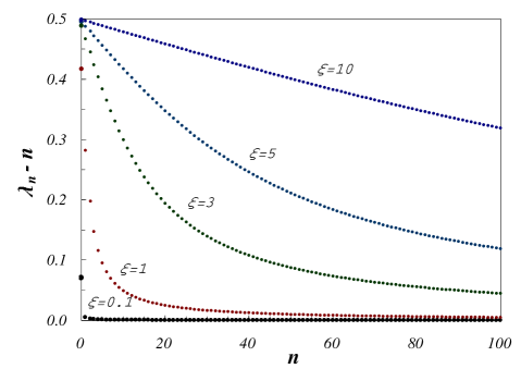
FIG. 1.: Eigenvalues $\lambda_{n}$ as calculated from Eq. (4) for various values of $\xi$. For comparison with the low $\xi$ limit discussed in the main text we show the deviation from the integer numbers. This picture depict how for large $\xi$ the eigenvalues get shifted close to semi-integer numbers. Notice also that for small $\xi$; $\lambda_{0}$ is clearly the only non integer eigenvalue.

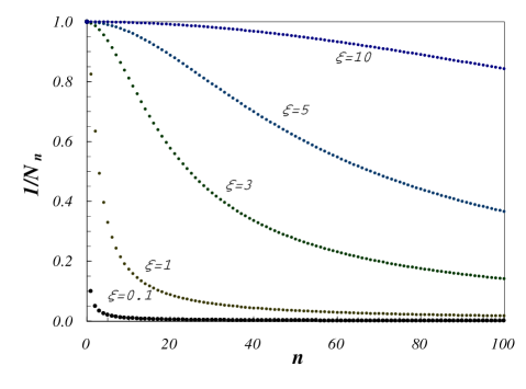
FIG. 2.: Mixing factors for the expansion (7) for different values of the parameter $\xi$. To make the effect for large $\xi$ visible we have introduced an arbitrary normalization where $N_{0}=1$. This amplifies the value of $1/N_{n}$ by a constant scaling. Of course, the real values satisfy the normalization condition. This figure shows how, for large $\xi$, the effective number of KK mass eigenmodes contributing into the weak eigenstate $\nu_{L}$ gets larger and those modes become almost equally suppressed, while for small $\xi$ the lightest mode ($n=0$) become the main component, with the decoupling of all other modes.

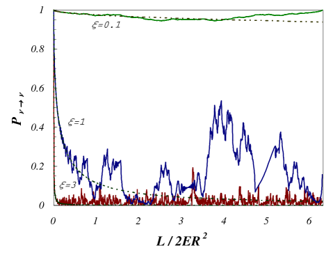
FIG. 3.: Exact survival probability for $\nu_{L}$ versus $L/2E$ in units of $R^{2}$ (as it is explicit in the argument) for three different values of $\xi$. Dotted lines represent the continuos approximation discused in the main text. Note that only the low $\xi$ limit has a periodic behaviour.

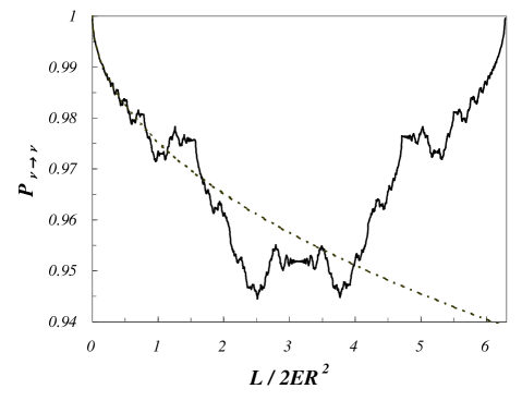
FIG. 4.: Here we show an amplification of the survival probability for the $\xi=0.1$ case showed in figure 3. Note the large number of wiggles produced by the oscillation of consecutive levels in Eq. (9). We also depict the continuos limit (dotted line) for comparison.

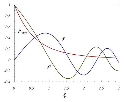
FIG. 5.: In this figure we plot the functions $\rho(\zeta)$ and $\vartheta(\zeta)$ that describe the slope of the survival probability $P_{surv}$ (which we also show) in the continuos limit where $\xi\geq 1$. The argument is the dimensionless parameter $\zeta=(\pi\xi^{2}/2R)\sqrt{L/2E}$ defined in the main text.

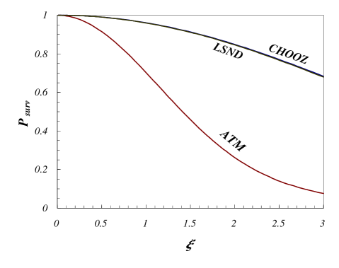
FIG. 6.: Dependance of the survival probability as a function of $\xi$ for the characteristic experimental values of $L/4E$, with $R=0.2~{}mm$.

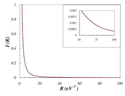
FIG. 7.: The function $I(R)$ versus $R$ for the experimental ratio $L/2E$ as in LSND. The window on the upper right shows an amplification of the region for large $R$, where $I(R)\leq 10^{-3}$.

REFERENCES

- [1] I. Antoniadis, Phys. Lett. B246 (1990) 377; I. Antoniadis, K. Benakli and M. Quirós, Phys. Lett. B331 (1994) 313; P. Horava and E. Witten, Nucl. Phys. B460 (1996) 506; idem B475(1996) 94; J. Lykken, Phys. Rev. D54 (1996) 3693. K.R. Dienes, E. Dudas and T. Gherghetta, Nucl. Phys. B436 (1998) 55; N. Arkani-Hamed, S. Dimopoulos and G. Dvali, Phys. Lett. B429 (1998) 263; Phys. Rev. D59 (1999) 086004; I. Antoniadis, S. Dimopoulos and G. Dvali, Nucl. Phys. B516 (1998) 70; N. Arkani-Hamed, S. Dimopoulos and J. March-Russell, hep-th/9809124.
- [2] For early proposals see: V. A. Rubakov and M. E. Shaposhnikov, Phys. Lett. B152 (1983) 136; K. Akama, in Lecture Notes in Physics, 176, Gauge Theory and Gravitation, Proceedings of the International Symposium on Gauge Theory and Gravitation, Nara, Japan, August 20-24, 1982, edited by K. Kikkawa, N. Nakanishi and H. Nariai, (Springer-Verlag, 1983), 267; M. Visser, Phys. Lett B159 (1985) 22; E.J. Squires, Phys. Lett B167 (1986) 286; G.W. Gibbons and D.L. Wiltshire, Nucl. Phys. B287 (1987) 717.
- [3] M. Gell-Mann, P. Ramond and R. Slansky, in Supergravity, eds. P. van Niewenhuizen and D.Z. Freedman (North Holland 1979); T. Yanagida, in Proceedings of Workshop on Unified Theory and Baryon number in the Universe, eds. O. Sawada and A. Sugamoto (KEK 1979); R. N. Mohapatra and G. Senjanović, Phys. Rev. Lett. 44, 912 (1980).
- [4] N. Arkani-Hamed and M. Schmaltz, Phys. Rev. D 61 (2000) 033005.
- [5] E. Witten, Invited talk at the Neutrino2000 Conference, Sudbury, Canada (June, 2000).
- [6] K.R. Dienes, E. Dudas and T. Gherghetta, Nucl. Phys. B557 (1999) 25; N. Arkani-Hamed, S. Dimopoulos, G. Dvali and J. March-Russell, hep-ph/9811448.
- [7] R. N. Mohapatra, S. Nandi and A. Pérez-Lorenzana, Phys. Lett B466 (1999) 115.
- [8] R. N. Mohapatra and A. Pérez-Lorenzana, Nucl. Phys. B576 (2000) 466.
- [9] C. Burgess, L. Ibanez and F. Quevedo, Phys. Lett. B447 (1999) 257.
- [10] G. Dvali and A.Yu. Smirnov, Nucl. Phys. B563 (1999) 63.
- [11] R. Barbieri, P. Creminelli and A. Strumia, hep-ph/0002199.
- [12] A. Faraggi and M. Pospelov, Phys. Lett. B458 (1999) 237; G. C. McLaughlin, J. N. Ng, Phys. Lett. B470 (1999) 157; nucl-th/0003023. A. Ioannisian, A. Pilaftsis, hep-ph/9907522.
- [13] A. Das and O. C. W. Kong, Phys. Lett. B470 (1999) 149; Y. Grossman and M. Neubert, Phys. Lett. B474 (2000) 361; A. Lukas and A. Romanino, hep-ph/0004130; E. Ma, M. Raidal and U. Sarkar, hep-ph/0006046.
- [14] A. Ioannissian and J. W. F Valle, hep-ph/9911349.
- [15] CHOOZ collaboration, M. Apollonio et al., Phys. Lett. B466 (1999) 415; Palo Verde collaboration, F. Boehm et al., hep-ex/0003022.
- [16] See the invited talk by T. Kajita, Neutrino2000 conference, Sudbury, Canada (2000).
- [17] D. Caldwell, R. N. Mohapatra and S. Yellin, to appear.