Cosmology and Hierarchy in Stabilized Warped Brane Models

Abstract

We examine the cosmology and hierarchy of scales in models with branes immersed in a five-dimensional curved spacetime subject to radion stabilization. When the radion field is time-independent and the inter-brane spacing is stabilized, the universe can naturally find itself in the radiation-dominated epoch. This feature is independent of the form of the stabilizing potential. We recover the standard Friedmann equations without assuming a specific form for the bulk energy-momentum tensor. In the models considered, if the observable brane has positive tension, a solution to the hierarchy problem requires the presence of a negative tension brane somewhere in the bulk. We find that the string scale can be as low as the electroweak scale. In the situation of self-tuning branes where the bulk cosmological constant is set to zero, the brane tensions have hierarchical values. In the case of a polynomial stabilizing potential no new hierarchy is created.

I. Introduction. It has recently been realized that the string scale can be much lower than the Planck scale and even close to the electroweak scale [1]. A low string scale provides new avenues on solving the hierarchy problem [2, 3]. The argument resides in the fact that a low string scale ($M_{X}$) may result in the apparent size of the Planck scale ($M_{Pl}$) due to the existence of a large volume ($R^{n}$) of compact extra dimensions, $M_{Pl}^{2}\sim M_{X}^{n+2}R^{n}$ [2]. Such a scenario may lead to a rich phenomenology at low energies and is thus testable at collider experiments [4].

Recently, a model involving just one extra dimension with a background $AdS_{5}$ metric was proposed by Randall and Sundrum [3] (see also Ref. [5]). In this scenario, two branes (one with positive tension and the other with negative tension) are located at the fixed points of an $S^{1}/\mathbf{Z_{2}}$ orbifold in a bulk with negative cosmological constant. An exponential hierarchy between the physical scales on the two branes is generated due to the curved spacetime, providing an explanation for the large hierarchy between the weak and Planck scales. The model is amenable to a holographic interpretation motivated by string theories [6]. However, the Randall-Sundrum model has some drawbacks. First, a perfect fine-tuning among the brane tensions and the bulk cosmological constant is needed to guarantee a static solution for the warped metric of spacetime. Mechanisms for stabilizing the brane locations via interactions between a bulk scalar field (called the radion) and the branes were suggested in [7] and elaborated in [8], where an elegant solution that accounts for the back-reaction of the scalar profile on the geometry is outlined. An overall fine-tuning equivalent to setting the four-dimensional cosmological constant to zero is still present. Second, it was found that the brane world may not lead to the standard cosmology [9, 10]. In particular, the Hubble parameter $H$ was found to be proportional to the matter density $\rho$ [10], in contradiction with the usual $H\sim\sqrt{\rho}$ behavior. Although this can be remedied by a fine-tuned cancellation between the brane tension and the bulk cosmological constant [11], only with a negative energy density on the observable brane is the standard cosmology recovered [12]. Much attention has been devoted to studying cosmology without an explicit stabilization mechanism [13]. The connection between radion stabilization and cosmology was explored in [12, 14, 15], and the standard cosmology can be obtained if the radion is time-dependent [12]. There have been attempts to modify the Randall-Sundrum model so that the observable brane has positive tension [16, 17, 18, 19], since the localization of matter and gauge fields on positive tension branes is well understood in string theory. An initial study with two positive tension branes was carried out [16], incorporating localized gravity in a noncompact $AdS_{5}$ geometry [20]. The necessary hierarchy can be generated between the Planck and electroweak scales by placing the hidden and observable branes at specific locations in the infinite dimension. We will refer to this as the Lykken-Randall model.

In this letter we examine the cosmology and hierarchy in models with radion stabilization. We shall adopt the formalism of Ref. [8] to stabilize the brane separation. We call this the Solution Generating Technique. We generalize it to the case of branes with arbitrary tensions and no relation between the metrics on either side of the branes. Using this technique we study the cosmology resulting from radion stabilization and find a cancellation between the bulk cosmological constant and the brane tension. This approach is rather different in philosophy from the one adopted in Refs. [14, 15, 19], where the bulk energy-momentum tensor extracted from the linearized field equations is chosen specifically to get the conventional cosmology. We obtain the important result that the stabilization of the inter-brane spacing can naturally lead to the cosmology of the radiation-dominated universe. Specifically, this is a consequence of requiring consistency in the equation of motion of the radion before and after perturbing the solutions by placing matter energy density on the observable brane. We argue that to obtain the complete evolution of our universe, a time-dependence of the radion field on the brane should be introduced. We speculate on the existence of some new dynamics that causes the transition from one epoch to the next.

Guided by cosmology, we explore the consequences on the hierarchy between the Planck and electroweak scales. As concrete examples, we study two classes of models. The first is the “self-tuning” model, motivated by recent attempts to solve the cosmological constant problem [21]. A dilaton-like coupling of a bulk scalar field with a brane was shown to result in a vanishing bulk cosmological constant. The result persists irrespective of the tension on the brane. This feature is referred to as self-tuning. The other model involves a Higgs-like radion potential, similar to that in [7]. In both models, the cosmology on the observable brane is independent of the configuration of branes and the potential that leads to radion stabilization. All that is required is some stabilizing potential and that the observable brane has positive tension. To generate the hierarchy of scales, at least one hidden brane with negative tension is required. The latter cannot be positioned at an orbifold fixed point.

The self-tuning brane model has the following properties:

1. The model illustrates the unique minimal configuration from which the hierarchy of scales can be obtained without fine-tuning. There are two positive tension branes (one of which is the observable brane), and one negative tension brane. The values of the brane tensions become hierarchical.

2. A dilatonic coupling between the branes and the bulk stabilizes the inter-brane spacings. Thus the radion may be identified with the dilaton.

3. The same coupling ensures self-tuning of the branes to be flat and the bulk cosmological constant to be zero. The tree-level contribution to the four-dimensional cosmological constant is eliminated. We will truncate the space to avoid curvature singularities.

The model with a Higgs-like radion potential possesses the following properties:

1. The minimal set-up to generate the scale hierarchy requires one positive tension observable brane and one negative tension hidden brane.

2. The extra dimension is linearly infinite with finite proper volume.

3. The radion field is unbounded above and leads to the bulk cosmological constant being unbounded below.

In Section II we present the Solution Generating Technique. Section III is devoted to studying the cosmology in a general setting. In Section IV we demonstrate a realization of a Lykken-Randall-like model with self-tuning branes. In Section V we perform a similar analysis but with a polynomial superpotential. We conclude in Section VI.

II. Solution Generating Technique. It is possible to use a gauged supergravity-inspired approach to reduce the nonlinear classical field equations of brane models with scalar-tensor gravity to a system of decoupled first order differential equations [8]. Using the technique of [8], the brane spacing can be stabilized. We assume the scalar field to be static to prevent the four-dimensional Planck mass from being time-dependent. The formalism is independent of whether the fifth dimension is compact or noncompact. We shall present the arguments for the case of a noncompact dimension.

We assume the presence of three 3-branes in the space $(-\infty,\infty)$, at $y_{0}=0\,$, $y_{1}$ and $y_{2}$ with the observable brane located at $y_{0}\,$. We will refer to the branes at $y_{1}$ and $y_{2}$ as hidden branes. The four-dimensional metric on the brane labelled by its position $y_{i}$ is $g_{\mu\nu}^{(i)}(x^{\mu})\equiv g_{\mu\nu}(x^{\mu},y=y_{i})\,$, where $g_{AB}$ is the five-dimensional metric and $A,B=0,1,2,3,5$ and $\mu,\nu=0,1,2,3$. We use the metric signature $(-,+,+,+,+)$. The five-dimensional gravitational action including a scalar field $\phi(y)$ is $S=S_{Gravity}+S_{Brane}$ with

$$S_{Gravity} = \int d^{4}x~{}dy~{}\sqrt{-g}\{{1\over 2\,\kappa^{2}}\,R-{1\over 4\,\kappa^{2}}\,\partial_{A}\phi\,\partial^{A}\phi-\Lambda(\phi)\}~{},~{}\,$$ (1)

$$S_{Brane} = -\sum_{i=0}^{2}\int d^{4}x~{}dy~{}\sqrt{-g^{(i)}}\>V_{i}(\phi)\,\delta(y-y_{i})~{},~{}\,$$ (2)

where $\kappa^{2}=8\,\pi\,G_{N}^{(5)}=M_{X}^{-3}$ is the five-dimensional coupling constant of gravity, $M_{X}$ is the Planck scale in five dimensions, $R$ is the curvature scalar and $V_{i}(\phi_{i})$ is the tension of the brane at $y_{i}$. $\Lambda(\phi)$ is the potential of the field $\phi$ in the bulk and is interpreted as the cosmological constant although it has a $\phi$-dependence. We allow it to be discontinuous at the branes, but continuous in each section. We write $\Lambda(\phi)$ as $\Lambda_{0}(\phi)\,$ if $\,y<0\,$, $\Lambda_{1}(\phi)\,$ if $\,0<y<y_{1}\,$ as $\Lambda_{2}(\phi)\,$ if $\,y_{1}<y<y_{2}\,$ and $\Lambda_{3}(\phi)\,$ if $\,y>y_{2}\,$ (see Fig. 1).

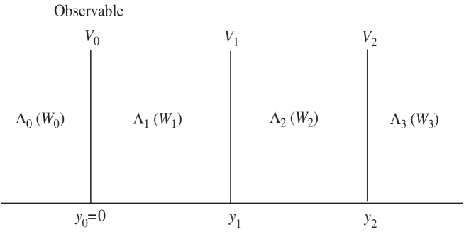
FIG. 1.: The configuration of branes in the bulk. $V_{i}$ is the tension of the brane at $y_{i}\,$, $\Lambda_{i}$ is the cosmological constant in the slice of $AdS_{5}$ between $y_{i-1}$ and $y_{i}$ and $W_{i}$ is the corresponding superpotential.

The five-dimensional Einstein equations arising from the above action are

$$G_{AB}\equiv R_{AB}-{1\over 2}g_{AB}R=\kappa^{2}\,T_{AB} = {1\over 2}\,(\partial_{A}\phi\,\partial_{B}\phi-{1\over 2}\,g_{AB}\,(\partial\phi)^{2})-\kappa^{2}\,g_{AB}\Lambda(\phi)$$ (4)

$$-\kappa^{2}\,\sum_{i=0}^{2}V_{i}(\phi)\sqrt{{g^{(i)}\over g}}~{}g_{\mu\nu}^{(i)}~{}\delta^{\mu}_{A}\delta^{\nu}_{B}~{}\delta(y-y_{i})\,,$$

where $R_{AB}$ is the five-dimensional Ricci tensor. The most general five-dimensional metric that respects four-dimensional Poincaré symmetry is

$$ds^{2}=e^{2\,A(y)}\ \eta_{\mu\nu}\ dx^{\mu}dx^{\nu}+(dy)^{2}~{}.~{}\,$$ (5)

The factor $e^{2\,A(y)}$ is commonly called a “warp factor”. The equation of motion of $\phi$ is

$$\phi^{\prime\prime}+4\,A^{\prime}\,\phi^{\prime} = 2\,\kappa^{2}\left({\partial\Lambda(\phi)\over\partial\phi}+\sum_{i=0}^{2}{\partial V_{i}(\phi)\over\partial\phi}~{}\delta(y-y_{i})\right)\,,$$ (6)

and the Einstein equations can be written as

$$A^{\prime\prime}=-{1\over 6}\phi^{\prime 2}-{\kappa^{2}\over 3}\sum_{i=0}^{2}V_{i}(\phi)~{}\delta(y-y_{i})\,,\ \ \ \ \ \ \ A^{\prime 2}={1\over 24}\phi^{\prime 2}-{\kappa^{2}\over 6}\Lambda(\phi)\ .$$ (7)

Here a prime denotes a derivative with respect to $y$. The jumps corresponding to the presence of the branes are

$$A^{\prime}\Big{|}^{y_{i}+\epsilon}_{y_{i}-\epsilon}=-{\kappa^{2}\over 3}V_{i}(\phi_{i})\,,\ \ \ \ \ \ \phi^{\prime}\Big{|}^{y_{i}+\epsilon}_{y_{i}-\epsilon}=2\,\kappa^{2}{\partial V_{i}(\phi)\over\partial\phi}\Bigg{|}_{\phi=\phi_{i}}\,,$$ (8)

where $\phi_{i}\equiv\phi(y_{i})$.

Let $W(\phi)$ be any sectionally continuous function (which we call the superpotential), with sectional functions $W_{i}(\phi)$ defined analogous to $\Lambda_{i}(\phi)$ (see Fig. 1). Taking

$$2\,\kappa^{2}\,\Lambda(\phi) = {1\over 2}\,\left(\partial W(\phi)\over\partial\phi\right)^{2}-{1\over 3}\,W(\phi)^{2}\,,$$ (9)

it is possible to show that a solution to the equations,

$$\phi^{\prime}={\partial W(\phi)\over\partial\phi}\,,\ \ \ \ \ \ A^{\prime}=-{1\over 6}\,W(\phi)\,,$$ (10)

subject to the constraints,

$$W(\phi)\Big{|}^{y_{i}+\epsilon}_{y_{i}-\epsilon}={2\,\kappa^{2}}V_{i}(\phi_{i})\,,\ \ \ \ \ \ {\partial W(\phi)\over\partial\phi}\Bigg{|}^{y_{i}+\epsilon}_{y_{i}-\epsilon}={2\,\kappa^{2}}{\partial V_{i}(\phi)\over\partial\phi}\Bigg{|}_{\phi=\phi_{i}}$$ (11)

is also a solution to the system of equations ($\ref{motion1}-\ref{bc}$). By solving Eq. (10) in the bulk and applying boundary conditions on the branes, we can determine the locations of the branes and hence their separation. Note that up to an arbitrary function $\sum_{n=2}^{\infty}\gamma_{n}\,(\phi-\phi_{i})^{n}\,$, the brane tension is completely determined by the superpotential and the value of $\phi$ on the brane,

$${2\,\kappa^{2}}\,V_{i}(\phi)=W_{i+1}(\phi_{i})-W_{i}(\phi_{i})+\left({\partial\over\partial\phi}(W_{i+1}(\phi)-W_{i}(\phi))\right)\Bigg{|}_{\phi=\phi_{i}}\,(\phi-\phi_{i})\,.$$ (12)

The solution involves fine-tuning even though it appears not to be the case. There are six constraints arising from the jump conditions on the three branes, but only five integration constants; the equations of motion and the jumps depend only upon $A^{\prime}(y)$ and $A^{\prime\prime}(y)$ thereby rendering the value of $A$ on one of the branes irrelevant [8].

III. Cosmology: General Considerations. Our starting point is the most general five-dimensional metric that preserves three-dimensional rotational and translational invariance. Thus, we adopt the cosmological principle of isotropy and homogeneity on the observable brane. However, $y$-dependence is maintained in the metric tensor since isotropy is broken in the fifth dimension due to the presence of branes. We consider the metric to be of the form

$$ds^{2}=-n^{2}(\tau,y)d\tau^{2}+a^{2}(\tau,y)d{\mathbf{x}^{2}}+b^{2}(\tau,y)dy^{2}.$$ (13)

The Einstein tensor for this metric is given by [10],

$$G_{00} = 3\left\{\frac{\dot{a}}{a}\left(\frac{\dot{a}}{a}+\frac{\dot{b}}{b}\right)-\frac{n^{2}}{b^{2}}\left(\frac{a^{\prime\prime}}{a}+\frac{a^{\prime}}{a}\left(\frac{a^{\prime}}{a}-\frac{b^{\prime}}{b}\right)\right)\right\},$$ (14)

$$G_{ij} = \frac{a^{2}}{b^{2}}\delta_{ij}\left\{\frac{a^{\prime}}{a}\left(\frac{a^{\prime}}{a}+2\frac{n^{\prime}}{n}\right)-\frac{b^{\prime}}{b}\left(\frac{n^{\prime}}{n}+2\frac{a^{\prime}}{a}\right)+2\frac{a^{\prime\prime}}{a}+\frac{n^{\prime\prime}}{n}\right\}$$ (16)

$$+\frac{a^{2}}{n^{2}}\delta_{ij}\left\{\frac{\dot{a}}{a}\left(-\frac{\dot{a}}{a}+2\frac{\dot{n}}{n}\right)-2\frac{\ddot{a}}{a}+\frac{\dot{b}}{b}\left(-2\frac{\dot{a}}{a}+\frac{\dot{n}}{n}\right)-\frac{\ddot{b}}{b}\right\},$$

$$G_{05} = 3\left(\frac{n^{\prime}}{n}\frac{\dot{a}}{a}+\frac{a^{\prime}}{a}\frac{\dot{b}}{b}-\frac{\dot{a}^{\prime}}{a}\right),$$ (17)

$$G_{55} = 3\left\{\frac{a^{\prime}}{a}\left(\frac{a^{\prime}}{a}+\frac{n^{\prime}}{n}\right)-\frac{b^{2}}{n^{2}}\left(\frac{\dot{a}}{a}\left(\frac{\dot{a}}{a}-\frac{\dot{n}}{n}\right)+\frac{\ddot{a}}{a}\right)\right\}.$$ (18)

where a dot denotes a derivative with respect to $\tau$. Note that the time-independent solution of the previous section corresponds to $a(\tau,y)=n(\tau,y)=e^{A(y)}$ and $b(\tau,y)=1$. We will maintain the assumption that the stabilizing potential is static, $\dot{b}=0\,$, and without loss of generality we set $b=1$. The energy-momentum tensor can be decomposed into two parts: a contribution from fields on the observable brane, ${\tilde{T}^{A}}_{\ \ B}=diag(-\rho_{0},p_{0},p_{0},p_{0},0)\,\delta(y)\,$, and the contribution ${\check{T}^{A}}_{\ \ B}$ of all other sources, i.e. bulk fields and matter on the other brane: ${T^{A}}_{B}={\tilde{T}^{A}}_{\ \ B}+{\check{T}^{A}}_{\ \ B}\,$. In the time-independent case, ${\tilde{T}^{A}}_{\ \ B}=diag(-V_{0},-V_{0},-V_{0},-V_{0},0)\,\delta(y)\,$. The jump conditions on the observable brane are [10]

$${{[a^{\prime}]}\over{a_{0}}}=-{{{\kappa}^{2}}\over 3}\rho_{0}\,\ \ \ {\rm{and}}\ \ \ {{[n^{\prime}]}\over{n_{0}}}={{{\kappa}^{2}}\over 3}\left(3\,p_{0}+2\,\rho_{0}\right),$$ (19)

where $[a^{\prime}]=a^{\prime}(+\epsilon)-a^{\prime}(-\epsilon)\,$, and functions with the subscript $0$ are evaluated on the observable brane. On taking the jump of the (0,5) component of Einstein’s equations, these conditions lead to the energy conservation equation,

$$\dot{\rho_{0}}+3(p_{0}+\rho_{0}){{\dot{a_{0}}}\over{a_{0}}}=0\,.$$ (20)

which is independent of $\dot{b}$. Taking the jump of the (5,5) component of Einstein’s equations, we get

$$3\,p_{0}\,{{{\langle a^{\prime}\rangle}}\over{a_{0}}}=\rho_{0}{{{\langle n^{\prime}\rangle}}\over{n_{0}}}+{[\check{T}_{55}]\over a_{0}}\,,$$ (21)

where

$$2\,{\langle a^{\prime}\rangle}=a^{\prime}(+\epsilon)+a^{\prime}(-\epsilon)\,.$$ (22)

We choose $n_{0}=1$, which amounts to identifying $\tau$ with time in conventional cosmology. Evaluating the (5,5) component of Einstein’s equations on either side of the observable brane and adding, we obtain

$$\left({\dot{a_{0}}\over a_{0}}\right)^{2}+{\ddot{a_{0}}\over a_{0}}=-{\kappa^{4}\over 36}\,\rho_{0}\,(\rho_{0}+3\,p_{0})-{\kappa^{2}\over 3}\,{\langle\check{T}_{55}\rangle}+{{{\langle a^{\prime}\rangle}}^{2}\over a_{0}^{2}}(1+{3\,p_{0}\over\rho_{0}})-{{\langle a^{\prime}\rangle}\,[\check{T}_{55}]\over\rho_{0}\,a_{0}^{2}}\,.$$ (23)

Usually, motivated by Hořava-Witten supergravity [22], a $\mathbf{Z_{2}}$ symmetry is imposed on the solutions. We simplify the above result by requiring the solutions to Einstein’s equations to obey a “$Z_{2}$ symmetry” in the neighborhood of the observable brane. By this we simply mean

$$W(\phi(+\epsilon))=-W(\phi(-\epsilon))\,,$$ (24)

because it leads to the warp factor being symmetric on either side of the observable brane. By a contextual abuse of terminology, we will call this a “local $Z_{2}$ symmetry”. (Of course, in no sense are we gauging the symmetry). To create a distinction, we will reserve the bold font for the “global” $\mathbf{Z_{2}}$ symmetry. We are therefore left with the following Friedmann-like equation:

$$\left({\dot{a_{0}}\over a_{0}}\right)^{2}+{\ddot{a_{0}}\over a_{0}}=-{\kappa^{4}\over 36}\,\rho_{0}\,(\rho_{0}+3\,p_{0})-{\kappa^{2}\over 3}\,{\langle\check{T}_{55}\rangle}\,,$$ (25)

derived in [10]. Let us emphasize the two assumptions on which our results will hinge. They are:

1. The extra dimension is assumed to be stable before studying cosmology.

2. The solutions satisfy a $Z_{2}$ symmetry in the immediate neighborhood of the observable brane, Eq. (24).

In finding the static solution of the previous section, we ignored the matter energy densities on the branes by assuming that they are negligible in comparison to the brane tensions. We now include their contribution as a perturbation to the “matter-less” solution. Thus, we can study the resulting cosmology by making the ansatz

$$\rho_{0}=\rho+V_{0}\,,\ \ \ \ p_{0}=p-V_{0}\,,$$ (26)

and Eq. (25) becomes

$$\left({\dot{a_{0}}\over a_{0}}\right)^{2}+{\ddot{a_{0}}\over a_{0}}={\kappa^{4}\over 18}\,V_{0}^{2}-\,{1\over 18}\,{\langle W(\phi_{0})^{2}\rangle}+{\kappa^{4}\over 36}\,V_{0}\,(\rho-3\,p)-{\kappa^{4}\over 36}\,\rho\,(\rho+3\,p)\,.$$ (27)

Here we have used

$$\kappa^{2}\,{\langle\check{T}_{55}\rangle}\,={1\over 6}\,{\langle W(\phi_{0})^{2}\rangle}\,,$$ (28)

which is obtained by inserting (9) and (10) into (4). Notice that $W(\phi_{0})$ is proportional to $A^{\prime}(0)$ and is therefore not well-defined. However, ${\langle W(\phi_{0})^{2}\rangle}$ is well-defined. On account of the local $Z_{2}$ symmetry and Eq. (12), we have

$$W(\phi(+\epsilon))^{2}=W(\phi(-\epsilon))^{2}=\kappa^{4}\,V_{0}^{2}\,.$$ (29)

The definition of ${\langle W(\phi_{0})^{2}\rangle}$ is analogous to Eq. (22), and we obtain

$${\langle W(\phi_{0})^{2}\rangle}=\kappa^{4}\,V_{0}^{2}\,.$$ (30)

This result relies heavily on the existence of the local $Z_{2}$ symmetry. The first two terms on the right hand side of Eq. (27) cancel out and we are left with

$$\left({\dot{a_{0}}\over a_{0}}\right)^{2}+{\ddot{a_{0}}\over a_{0}}={\kappa^{4}\over 36}\,V_{0}\,(\rho-3\,p)-{\kappa^{4}\over 36}\,\rho\,(\rho+3\,p)\,.$$ (31)

The leading term on the right-hand side reproduces the standard cosmology if we make the identification, $\kappa^{4}V_{0}=6/M_{Pl}^{2}$. It is essential for the observable brane to possess positive tension to arrive at the correct Friedmann equations in spite of an explicit radion stabilization. Furthermore, a specific form of the bulk energy-momentum tensor was not chosen to implement the cancellation. Beyond the conventional fine-tuning one does not need additional machinery to obtain the usual cosmology.

In introducing the perturbation (26), it is no longer obvious that the solutions remain consistent. Let us consider the equation of motion of $\phi$. On the observable brane it is

$$\phi^{\prime\prime}+\left(3\,\frac{a^{\prime}}{a}+\frac{n^{\prime}}{n}\right)\,\phi^{\prime}=2\,\kappa^{2}{\partial\over\partial\phi}(\Lambda(\phi)+V_{0}(\phi))\,,$$ (32)

where all quantities are evaluated at $y_{0}$. We started with just tension on the branes and demanded that the radion stabilize the configuration of branes. Having obtained this static solution we then proceeded to consider the effect of matter on the observable brane. Let us require that the positions of the branes be unchanged by appealing to the stability of such a scenario. This is equivalent to saying that $\phi$ and $\Lambda(\phi)$ are unchanged before and after the introduction of the matter energy density. Then consistency requires,

$$\left(3\,\frac{a^{\prime}}{a}+\frac{n^{\prime}}{n}\right)\Big{|}_{0\,,\,Static}=\left(3\,\frac{a^{\prime}}{a}+\frac{n^{\prime}}{n}\right)\Big{|}_{0\,,\,Perturbed}\ \,.$$ (33)

Again, using the local $Z_{2}$ symmetry and the jump conditions (19), we get

$$-\,{\kappa^{2}\over 2}\,V_{0}-{\kappa^{2}\over 6}\,V_{0}=-\,{\kappa^{2}\over 2}\,(\rho+V_{0})+{\kappa^{2}\over 6}\,(3\,p+2\,\rho-V_{0})\,,$$ (34)

which leads to the condition for a radiation-dominated (RD) universe,

$$\rho=3\,p\,.$$ (35)

The interpretation of the above constraint is interesting. When matter on the observable brane is radiation, the inter-brane spacing is identical to the case when there is no matter on the brane. Conversely, when the brane location is unaffected by the matter-perturbation, the universe is RD. This observation is consistent with the fact that the radion couples to the trace of the energy-momentum tensor [12, 15], which is zero for radiation. It may be possible to identify the process of radion stabilization with inflation and reheating and the time at which the inter-brane spacing becomes stable marks the end of reheating. The RD universe then ensues.

To study cosmology at lower temperatures, we need the radion to be time-dependent. The radion can be written as

$$\phi(\vec{x},t,y)=\phi(\vec{x},t)\,\phi(y)\,,$$ (36)

the form of which encodes the requirement that the bulk remain static (so as to maintain a non-fluctuating Planck scale). In our previous analysis we have set $\phi(\vec{x},t)=1$. The Solution Generating Technique is still applicable provided the derivatives of $\phi(\vec{x},t)$ with respect to $\vec{x}$ and $t$ are negligible. It is conceivable that $\phi(\vec{x},t)$ plays a role in the evolution from a RD universe to a matter-dominated universe and is perhaps responsible for the transition to an accelerating universe as in quintessence models [23].

IV. Self-tuning Flat Branes. In this section we study the case where the superpotential takes on the form of the tree-level dilaton coupling. This will lead us to the case of a vanishing bulk cosmological constant [21]. The resulting $\phi$ has two singularities at finite distances on either side of the observable brane. We will describe how these singularities can be dealt with.

Consider a superpotential of the exponential form

$$W_{i}(\phi) = \omega_{i}\,e^{-\beta\phi}\,,$$ (37)

for which

$$12\,\kappa^{2}\,\Lambda_{i}(\phi)=(3\,\beta^{2}-2)\,\omega_{i}^{2}\,e^{-2\beta\phi}\,.$$ (38)

For $\beta^{2}=2/3$, we have the important result that $\Lambda=0$ [21]. Henceforth, we restrict ourselves to this choice. When we have not committed to the sign of $\beta$, we will leave it explicit in the equations. With $\beta^{2}=2/3$ the branes are flat and will remain so, independent of the matter on them (hence the expression “self-tuning flat branes”).

As we pointed out in Sec. II, the tension on the branes is fixed by the superpotential. As long as the tension satisfies Eq. (12), it is irrelevant what functional form it takes, i.e. the particular form of the tension we choose is simply a calculational device with no bearing on the physics. We take

$${12\,\kappa^{2}}\,V_{i}(\phi) = (\omega_{i+1}-\omega_{i})\,e^{-\beta\phi}\,.$$ (39)

Then it can be shown that

$$\phi(y)={1\over\beta}\ln[{-(\sum_{i=0}^{2}k_{i}\,|y-y_{i}|+k_{c}\,y)+c}]\,,\ \ \ \ \ A(y)={1\over{6\,\beta}}\phi(y)+h\,,$$ (40)

where $k_{i}=(\omega_{i+1}-\omega_{i})/3\,$ and $k_{c}=(\omega_{0}+\omega_{3})/3\,$. Here $c$ is a constant that can be fixed by the boundary conditions on any brane. Conventionally, the constant $h$ is set to zero, but its value does not affect the hierarchy of scales. Let us call the argument of the logarithm in Eq. (40), $f(y)$. Then,

$$f(y)\equiv e^{\beta\phi(y)}=-{2\over 3}\,\omega_{i}\,y+c_{i}\ \ \ {\rm{for}}\ \ \ y_{i-1}\leq y\leq y_{i}\,,$$ (41)

where $c_{i}$ is a constant of integration. Note that when $\omega_{i}$ is positive (negative), $e^{\beta\phi}$ falls (rises) linearly. When $f$ vanishes, $\phi$ diverges and the warp factor vanishes. The space collapses to a point at these locations and these points can be identified with horizons. Assume that the horizons at $y_{min}$ and $y_{max}$ are such that $y_{min}<0$ and $y_{max}>y_{2}$. We will truncate the space at the horizons. There is much debate about the justification of this procedure if one hopes to solve the cosmological constant problem. It has been claimed that the four-dimensional cosmological constant vanishes only when the singularities contribute to the vacuum energy [24]. If negative tension branes are introduced at the singularities, it is possible to set the four-dimensional cosmological constant to zero, but not without fine-tuning [24]. Attempts have been made to find bulk potentials such that self-tuning remains while simultaneously removing the singularities. It has been found [25] that if the singularities are removed, gravity is no longer localized and the four-dimensional Planck scale diverges. We will content ourselves with having $\Lambda=0$ as an improvement to the cosmological constant problem. We assume the presence of some dynamics at the singularities that does not affect the global properties of the solution and may resolve the problem of fine-tuning. So that $\phi$ be well-defined and accommodate our assumptions, we must impose the constraint,

$$\sum_{i=0}^{2}k_{i}>|k_{c}|\ \Rightarrow\begin{array}[]{ll}\ \omega_{3}>0\ \ {\rm{iff}}\ \ k_{c}<0\,,\ \ \ \ \ \omega_{0}<0\ \ {\rm{iff}}\ \ k_{c}>0\,.\end{array}$$ (42)

Now we can calculate the four-dimensional Planck scale in terms of the five-dimensional Planck scale $M_{X}$,

$$M_{Pl}^{2}=M_{X}^{3}\,\int e^{2\,A(y)}\,dy$$ (43)

to be

$$M_{Pl}^{2}=M_{X}^{3}\,{e^{2\,h}}\,\left[({1\over\omega_{1}}-{1\over\omega_{0}})\,e^{\phi_{0}/\beta}+({1\over\omega_{2}}-{1\over\omega_{1}})\,e^{\phi_{1}/\beta}+({1\over\omega_{3}}-{1\over\omega_{2}})\,e^{\phi_{2}/\beta}\right]\,.$$ (44)

We recall that the electroweak scale ($M_{EW}$) can be generated from the five-dimensional Planck scale $M_{X}$ via the square root of the warp factor [3],

$$M_{EW}\simeq M_{X}\,e^{A(0)}=M_{X}\,e^{\phi_{0}/(6\,\beta)}\,.$$ (45)

Two branes geometry: Let us specialize to the case of just two branes. The formulae for the case of three branes apply by simply dropping the terms corresponding to the extra indices. We choose

$$W_{1}(\phi)=-W_{0}(\phi)=\omega_{1}\,e^{-\beta\phi}\,,\ \ \ W_{2}(\phi)=\omega_{2}\,e^{-\beta\phi}\,.$$ (46)

As required by cosmology, $W(\phi)^{2}$ has a local $Z_{2}$ symmetry about the observable brane. From Eq. (39), we need to impose $\omega_{1}>0$ so that the observable brane has positive tension. The four-dimensional Planck scale is

$$M_{Pl}^{2}=M_{X}^{3}\left[{2\over\omega_{1}}\,e^{\phi_{0}/\beta}+({1\over\omega_{2}}-{1\ \over\omega_{1}})\,e^{\phi_{1}/\beta}\right]\,.$$ (47)

From Eq. (41), one can readily see that $e^{\phi_{0}/\beta}>e^{\phi_{1}/\beta}$. Since $\omega_{0}=-\omega_{1}<0\,$, the constraint from Eq. (42) requires $\omega_{2}>\omega_{1}\,$. This implies that the hidden brane has positive tension. Therefore, the second term in Eq. (47) makes a negative contribution to $M_{Pl}^{2}$. The first term must be the dominant contribution for $M_{Pl}^{2}>0$ and $\phi_{0}/\beta\gg\phi_{1}/\beta$ must be satisfied, where “$\gg$” implies a hierarchy of at most two orders of magnitude. We would like the fundamental parameters $M_{X}$ and $\omega_{i}$ to be roughly of the same order of magnitude to avoid a fine-tuned hierarchy of scales. We obtain

$$M_{Pl}\simeq M_{X}\,e^{\phi_{0}/(2\,\beta)}\,,\quad M_{Pl}/M_{EW}\simeq e^{\phi_{0}/(3\,\beta)}.$$ (48)

We need $\phi_{0}/(3\beta)\simeq 37$ to get the correct hierarchy with $M_{Pl}\simeq 10^{19}$ GeV and $M_{EW}\simeq 10^{3}$ GeV. This leads to $M_{X}\simeq 10^{-5}$ GeV. Interpreting $M_{X}$ as the string scale is now impossible. The difficulty arises because both the Planck and electroweak scales are determined by the value of $\phi$ on the observable brane. Any self-tuning brane model with only two branes shares this problem; $\phi$ will always be required to have its maximum value on the observable brane because of the local $Z_{2}$ symmetry.

Three branes geometry: We construct a model with three branes in which the Planck scale will be generated by the value of $\phi$ on a neighboring brane. We investigate the superpotential

$$W_{1}(\phi)=-W_{0}(\phi)=\omega_{1}\,e^{-\beta\phi}\,,\ \ \ W_{2}(\phi)=\omega_{2}\,e^{-\beta\phi}\,,\ \ \ W_{3}(\phi)=\omega_{3}\,e^{-\beta\phi}\,.$$ (49)

Notice that $W(\phi)^{2}$ has a local $Z_{2}$ symmetry. We leave the sign of the tensions of the hidden branes unspecified for the time being. The Planck scale is given by Eq. (44) with $\omega_{0}=-\omega_{1}$. Again, from Eq. (41), $e^{\phi_{0}/\beta}>e^{\phi_{1}/\beta}$. The only way of getting $e^{\phi_{2}/\beta}>e^{\phi_{0}/\beta}$ is by choosing $\omega_{2}<0$. From Eq. (39) we can see that the brane at $y_{1}$ must have negative tension. Since there are no more branes in the bulk, so that $e^{\phi/\beta}\to 0$ at $y_{max}$, we must have $\omega_{3}>0$. Thus, the brane at $y_{2}$ has positive tension. This situation calls for two hidden branes, one with positive and the other with negative tension in a unique configuration. The configuration of branes, the profiles of $e^{\beta\phi}$ and the warp factor $e^{2\,A(y)}=\sqrt{e^{\beta\phi}}$ are shown in Fig. 2. The model resembles the “$+-+$” model of Ref. [17], which however is not derived by imposing constraints from radion stabilization and has a compactification on $S^{1}/{\mathbf{Z_{2}}}$ .

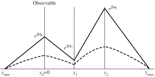
FIG. 2.: The profile of $e^{\beta\phi}$ (solid) and the warp factor (dashed) in the case of self-tuning branes. In regions where $\omega_{i}$ is positive (negative), $e^{\beta\phi}$ falls (rises) linearly. The brane at $y_{1}$ must have negative tension so that $e^{\beta\phi_{2}}>e^{\beta\phi_{0}}$.

If we assume $M_{X}$ and $\omega_{i}$ to be of the same order of magnitude and $\phi_{2}/\beta\gg\phi_{1}/\beta\,,\ \phi_{0}/\beta$, then

$$M_{Pl}\simeq M_{X}\,e^{\phi_{2}/(2\,\beta)}\,,\quad M_{Pl}/M_{EW}\simeq e^{{(\phi_{2}-\phi_{0}/3)}/(2\,\beta)}\,.$$ (50)

To obtain the correct hierarchy we must have $(\phi_{2}-\phi_{0}/3)/(2\beta)\simeq 37$. By choosing appropriate values of $\phi_{0}$ and $\phi_{2}$, we are able to generate the hierarchy between $M_{Pl}$ and $M_{EW}$ for essentially any value of $M_{X}$ in between. For illustration, we present two particularly interesting examples. First, we can achieve $M_{X}\simeq M_{Pl}$ by taking $\phi_{2}\to 0$ (or any other value that yields $e^{\phi_{2}}\simeq{\cal O}(1)$), corresponding to $\phi_{0}/\beta\simeq-220$. At the other extreme, we can obtain $M_{X}\simeq M_{EW}$ by taking $\phi_{0}\to 0$, corresponding to $\phi_{2}/\beta\simeq 75$. We mention in passing that the solution that leads to $M_{X}\simeq M_{EW}$ is slightly less fine-tuned in terms of the difference in $|\phi_{i}|$ than the one leading to the high energy string scale. A lighter string scale is preferred in this sense.

A couple of points are noteworthy. The solution presented represents the unique minimal configuration that allows for the generation of the hierarchy of scales without fine-tuning. The negative tension brane must lie between two positive tension branes. In the case at hand, it is not possible to place the negative tension brane at the fixed point of an orbifold. The only possible discrete symmetry that can be imposed on $R^{1}$ is $\mathbf{Z_{2}}$. If we considered the orbifold $R^{1}/\mathbf{Z_{2}}$ with a fixed point at $y_{1}$, we would not be able to satisfy $e^{\phi_{2}/\beta}>e^{\phi_{0}/\beta}$. Since the negative tension brane is not at an orbifold fixed point, the radion may have a problem with positivity of energy [26]. This is an unpleasant circumstance but nevertheless, we assume the model to be theoretically feasible. More problematic is the introduction of a new hierarchy problem. By inspecting Eq. (39) it can be seen that due to the exponential dependence of the brane tensions on $\phi\,$, a large hierarchy is generated between the values of the tensions for even moderately different values of $\phi$.

V. Polynomial Superpotentials. Here we consider the type of superpotential that leads to the stabilization mechanism suggested in [7]. In [8] it was demonstrated that a quadratic superpotential results in the mechanism of [7]. We have studied all geometries with two positive tension branes (with bounded and unbounded $\phi$) and numerically scanned the parameter space. As in the model of the previous section, we find that it is not possible to generate the appropriate scale hierarchy with only positive tension branes. We therefore study a model with two branes where the hidden brane has negative tension. The first column of Table I shows our particular choice of the polynomial superpotential, which is guided by cosmology discussions with a $Z_{2}$ symmetry. For simplicity, we have multiplied $y$ by $M_{X}$ to make it dimensionless. The second and third columns of Table I present the static solution to Einstein’s equations, where $a_{0}$ is an irrelevant integration constant which we set to zero. We find it necessary for the radion to be unbounded for $y>y_{1}$. This leads to $\Lambda(\phi)$ being unbounded below. This is often seen in $AdS$ supergravity and offers no threat to the model [8]. In the region $y<0$, the radion may or may not be bounded without affecting the hierarchy. We will choose it to be unbounded in both regions, thus making the value of $\phi_{0}$ a global minimum. Figure 3 illustrates the profiles of $\phi$ and $A(y)$ in the bulk.

$W(\phi)/M_{X}$	$\phi(y)$	$A(y)$	Region
$(\eta-\phi^{2})$	$\phi_{0}\,e^{2\,|y|}$	$a_{0}+{1\over 6}\,\eta\,|y|-{\phi_{0}^{2}\over 24}\,e^{4\,|y|}$	$y<0$
$-(\eta-\phi^{2})$	$\phi_{0}\,e^{2\,y}$	$a_{0}+{1\over 6}\,\eta\,y-{\phi_{0}^{2}\over 24}\,e^{4\,y}$	$0<y<y_{1}$
$-(\xi-\phi^{2})$	$\phi_{0}\,e^{2\,y}$	$a_{0}+{1\over 6}\,\eta\,y_{1}+{1\over 6}\,\xi\,(y-y_{1})-{\phi_{0}^{2}\over 24}\,e^{4\,y}$	$y_{1}<y$

TABLE I.: The solution to Einstein’s equations in a model with a polynomial superpotential.

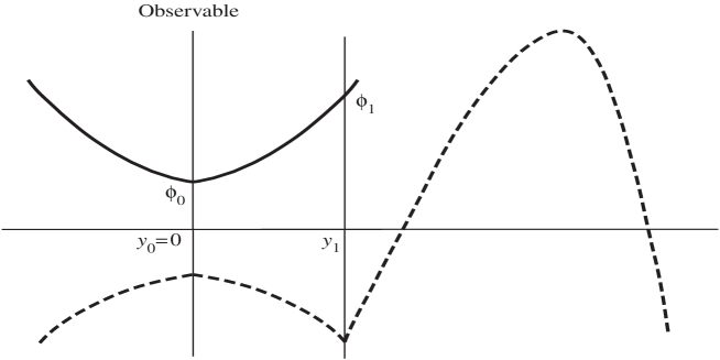
FIG. 3.: Representative configurations of the radion (solid) and $A(y)$ (dashed) in the case of a quadratic superpotential. To generate the appropriate hierarchy of scales, the hidden brane at $y_{1}$ is required to have negative tension.

The location of the hidden brane is

$$y_{1}=\ln\left({{\phi_{1}\over\phi_{0}}}\right)^{1\over 2}\,.$$ (51)

The electroweak scale is

$$M_{EW}\simeq M_{X}\,e^{A(0)}=M_{X}\,e^{-{\phi_{0}^{2}\over 24}}\,.$$ (52)

The Planck scale is given by

$$\left(2\,{M_{Pl}\over M_{X}}\right)^{2}=\left({\phi_{0}^{2}\over 12}\right)^{-{\xi\over 12}}\,\Gamma\left({\xi\over 12},{\phi_{1}^{2}\over 12},\infty\right)+\left({\phi_{0}^{2}\over 12}\right)^{-{\eta\over 12}}\,\left[\Gamma\left({\eta\over 12},{\phi_{0}^{2}\over 12},{\phi_{1}^{2}\over 12}\right)+\,\Gamma\left({\eta\over 12},{\phi_{0}^{2}\over 12},{\infty}\right)\right]\,,$$ (53)

where the generalized incomplete gamma function is $\Gamma(a,x,y)\equiv\int_{x}^{y}t^{a-1}\,e^{-t}\,{dt}\,$. Consistency conditions imposed by positivity of the tension of the observable brane and the profile of the radion are $\eta<\phi_{0}^{2}<\phi_{1}^{2}\,$. When the correct hierarchy is generated, by far the dominant contribution to $M_{Pl}$ comes from the first term on the right-hand-side of Eq. (53). This term is the integral over the space $y>y_{1}$. The condition under which this integral dominates is $\phi_{0}^{2}<\phi_{1}^{2}<\xi$. Then $\eta<\xi\,$, and the brane at $y_{1}$ has negative tension. If we choose $\eta>\xi\,$, the brane will have positive tension, but the desired hierarchy of scales cannot be obtained. It is not possible to place the negative tension brane at an orbifold fixed point because the space beyond $y_{1}$ is crucial for generating the scale hierarchy. We can again obtain a solution with a string scale anywhere between $M_{EW}$ and $M_{Pl}$.

As an explicit realization that solves the hierarchy problem, consider the following choice of parameters: $\eta=12\,,\phi_{0}^{2}=24\,,\phi_{1}^{2}=100\,,\xi=450$. The largest hierarchy among these parameters is only ${\cal O}(10)$. With the above choice, $M_{Pl}\approx 10^{15}\,M_{X}\,$ and $M_{EW}\approx 10^{-1}\,M_{X}\,$.

VI. Conclusion. We have studied the cosmology and hierarchy in models with branes immersed in a five-dimensional curved spacetime subject to radion stabilization. We found that when the radion field is time-independent and the inter-brane spacing is stabilized, consistent solutions that reproduce the conventional cosmological equations can naturally lead to a radiation-dominated universe. This feature is independent of the form of the stabilizing potential. The only assumption made is that the warp factor is symmetric on either side of the observable brane.

Guided by constraints on the stabilizing superpotential imposed by cosmology, we proceeded to consider solutions to the hierarchy problem. We insisted that the observable brane have positive tension and considered a noncompact fifth dimension. We examined two classes of models— an exponential and a polynomial superpotential. We find that these scenarios generically require at least one hidden brane with negative tension to get the correct hierarchy. This brane cannot be located at the fixed point of an orbifold. In both models, the correct hierarchy between the electroweak and Planck scales can be obtained for any value of the string scale, including the interesting result $M_{X}\simeq M_{EW}$, without fine-tuning. The exponential superpotential leads to the interesting case of a vanishing bulk cosmological constant, referred to as a self-tuning brane model. As in [21], we needed to truncate the space to avoid curvature singularities. In this model, generating the hierarchy of scales results in the brane tensions becoming hierarchical. In the case of a polynomial superpotential no new hierarchy is created.

Acknowledgments. We thank C. Goebel for discussions. This work was supported in part by a DOE grant No. DE-FG02-95ER40896, in part by the Wisconsin Alumni Research Foundation, and in part by the Fermi National Accelerator Laboratory, which is operated by the Universities research Association, Inc., under contract No. DE-AC02-76CHO3000.

REFERENCES

- [1] I. Antoniadis, Phys. Lett. B246, 377 (1990); J. D. Lykken, Phys. Rev. D54, 3693 (1996); G. Shiu and S.H.H. Tye, Phys. Rev. D58, 106007 (1998).
- [2] N. Arkani-Hamed, S. Dimopoulos and G. Dvali, Phys. Lett. B429, 263 (1998); I. Antoniadis, N. Arkani-Hamed, S. Dimopoulos and G. Dvali, Phys. Lett. B436, 257 (1998).
- [3] L. Randall and R. Sundrum, Phys. Rev. Lett. 83, 3370 (1999).
- [4] G.F. Giudice, R. Rattazzi and J.D. Wells, Nucl. Phys. B544, 3 (1999); E. A. Mirabelli, M. Perelstein and M. Peskin, Phys. Rev. Lett 82, 2236 (1999); T. Han, J.D. Lykken and R.-J. Zhang, Phys. Rev. D59, 105006 (1999); J. Hewett, Phys. Rev. Lett 82, 4765 (1999); T. Rizzo, Phys. Rev. D59, 115010 (1999).
- [5] M. Gogberashvili, hep-ph/9812296; Europhys. Lett. 49, 396 (2000).
- [6] H. Verlinde, hep-th/9906182.
- [7] W. Goldberger and M. Wise, Phys. Rev. Lett. 83, 4922 (1999).
- [8] O. DeWolfe, D. Freedman, S. Gubser and A. Karch, hep-th/9909134.
- [9] A. Lukas, B.A. Ovrut, K.S. Stelle and D. Waldram, Phys. Rev. D59, 086001 (1999); N. Kaloper and A. Linde, Phys. Rev. D59, 101303 (1999); A. Lukas, B.A. Ovrut, and D. Waldram, Phys. Rev. D60, 086001 (2000); Phys. Rev. D61, 023506 (2000); D.J.H. Chung and K. Freese, Phys. Rev. D61, 023511 (2000).
- [10] P. Binétruy, C. Deffayet and D. Langlois, Nucl. Phys. B565, 269 (2000).
- [11] C. Csáki, M. Graesser, C. Kolda and J. Terning, Phys. Lett. B462, 34 (1999); J. Cline, C. Grojean and G. Servant, Phys. Rev. Lett. 83, 4245 (1999).
- [12] C. Csáki, M. Graesser, L. Randall and J. Terning, hep-ph/9911406.
- [13] H. A. Chamblin and H. S. Reall, Nucl. Phys. B562, 133 (1999); T. Nihei, Phys. Lett. B465, 81 (1999); N. Kaloper, Phys. Rev. D60, 123506 (1999); H. B. Kim and H. D. Kim, Phys. Rev. D61, 064003 (2000); P. Binétruy, C. Deffayet and U. Ellwanger, Phys. Lett. B477, 285 (2000); E. Flanagan, H. Tye and I. Wasserman, hep-ph/9909373; hep-ph/9910498; H. Stoica, H. Tye and I. Wasserman, hep-ph/0004126; R. Mohapatra, A. Pérez-Lorenzana and C. A. de S. Pires, hep-ph/0003328; J. E. Kim and B. Kyae, Phys. Lett. B486, 165 (2000); J. Lesgourgues, S. Pastor, M. Peloso and L. Sorbo, hep-ph/0004086.
- [14] P. Kanti, I. Kogan, K.A. Olive and M. Pospelov, Phys. Lett. B468, 31 (1999); H. B. Kim, Phys. Lett. B478, 285 (2000).
- [15] P. Kanti, I. Kogan, K.A. Olive and M. Pospelov, Phys. Rev. D61, 106004 (2000).
- [16] J. D. Lykken and L. Randall, JHEP 0006:014 (2000).
- [17] I. Kogan, S. Mouslopoulos, A. Papazoglou, G. Ross and J. Santiago, hep-ph/9912552.
- [18] T. Li, hep-th/9911234; hep-th/9912182.
- [19] P. Kanti, K.A. Olive and M. Pospelov, hep-ph/0002229; hep-ph/0005146.
- [20] L. Randall and R. Sundrum, Phys. Rev. Lett. 83, 4690 (1999).
- [21] N. Arkani-Hamed, S. Dimopoulos, N. Kaloper and R. Sundrum, hep-th/0001197; S. Kachru, M. Schulz and E. Silverstein, hep-th/0001206; hep-th/0002121.
- [22] P. Hořava and E. Witten, Nucl. Phys. B460, 506 (1996).
- [23] I. Zlatev, L. Wang and P. Steinhardt, Phys. Rev. Lett. 82, 896 (1999); C. Armendariz-Picon, V. Mukhanov and P. Steinhardt, astro-ph/0004134.
- [24] S. Förste, Z. Lalak, S. Lavignac and H.P. Nilles, hep-th/0002164.
- [25] C. Csáki, J. Erlich, C. Grojean and T. Hollowood, hep-th/0004133.
- [26] E. Witten, hep-ph/0002297; L. Pilo, R. Rattazzi and A. Zaffaroni, hep-th/0004028.