Measuring the neutrino mass using intense photon and neutrino beams

Abstract

We compute the cross section for neutrino-photon scattering taking into account a neutrino mass. We explore the possibility of using intense neutrino beams, such as those available at proposed muon colliders, together with high powered lasers to probe the neutrino mass in photon-neutrino collisions.

I Introduction

Several experiments studying solar, atmospheric and reactor neutrinos accumulated over the past several years provide an increasing body of evidence supporting the existence of neutrino oscillations conrad ; SLAC . The existence of neutrino oscillations will require a significant departure from the the Standard Model. Oscillations imply that at least one of the neutrinos is massive and that lepton number is not conserved. The oscillation probability depends on the mass difference between the oscillating neutrinos and is insensitive to the value of the neutrino mass. The possible values of the mass difference are small, lying typically in the range $10^{-5}$ to $10^{-3}$ eV. The experimental limits on the muon and tau neutrino masses come from kinematic distributions in weak decays. They are pdg $m_{\nu_{\mu}}<0.17$  MeV and $m_{\nu_{\tau}}<18.2$  MeV. If oscillations do occur, the mass of $\nu_{\tau}$ is expected to be within less than 1 eV from that of $\nu_{\mu}$, and, therefore, the determination of the muon neutrino mass is of special importance. The experimental measurement setting a limit on the $\nu_{\mu}$ mass is based on the kinematics of pion decay at rest and is dominated by difficult to control systematic effects. Consequently, it is of special particular interest to explore all possible other processes that may be sensitive to the neutrino mass.

We note that neutrino photon scattering, with and without photon production in both the non-relativistic and relativistic regimes, has been studied extensively within the standard model DR . Astrophysical implications have been considered in, for example, teplitz and the effect of scattering in a background magnetic field has also been investigated sha ; chyi .

This paper attempts to exploit the fact that these cross sections vary as the square of the neutrino mass to determine whether it might be possible to measure the elastic scattering cross section for values of the muon neutrino mass below its current limit cited above. We find that it is not possible with neutrinos from a facility on the order of the muon collider under current discussion. We provide an indication of the kind of facility that would support such a measurement. In Section 2 we derive the needed formulae and evaluate the cross section and in Section 3 we sketch the scope of an experiment to measure $m_{\nu}$. This is followed by a discussion.

II Contributions to the $\bm{\gamma\nu\to\gamma\nu}$ cross section

II.1 ${\bm{Z}^{0}}$ exchange

A typical contribution to the amplitude for photon-neutrino scattering due to a fermion loop with $Z^{0}$ exchange is illustrated in Fig. 1. Because of Yang’s theorem Yang , this amplitude will contain a factor of the neutrino mass $m_{\nu}$ GellMann . For center of mass energies low compared to the $Z^{0}$ mass,

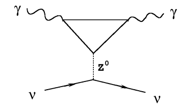
Figure 1: A typical fermion triangle diagram for the $\gamma\nu\to\gamma\nu$ amplitude is shown. The particle in the loop can be an electron, up quark, down quark, etc.

the effective neutral current coupling between the charged fermions and neutrinos due to $Z^{0}$ exchange is

$${\cal L}_{Z}=\frac{G_{F}}{\sqrt{2}}\bar{\nu}(x)\gamma_{\mu}(1+\gamma_{5})\nu(x)\bar{f}(x)\gamma_{\mu}\left((t_{3}(f)-2q_{f}\sin^{2}\theta_{W})+t_{3}(f)\gamma_{5}\right)f(x)\,,$$ (1)

where $t_{3}(f)$ is the third component of the fermion weak isospin, and $q_{f}$ is the fermion charge in units of the proton charge. When the coupling, Eq. (1) is combined with the fermion electromagnetic coupling, only the weak axial vector contribution survives. For a particular fermion, the triangle amplitude takes the form

$${\cal A}_{Z}=\frac{G_{F}}{\sqrt{2}}\bar{u}(p_{2})\gamma_{\mu}(1+\gamma_{5})u(p_{1})t_{3}(f){\cal M}_{\lambda\rho,\mu}\varepsilon_{\lambda}(k_{1})\varepsilon_{\rho}^{*}(k_{2})\,,$$ (2)

with

$${\cal M}_{\lambda\rho,\mu}=\frac{4\alpha q_{f}^{2}C_{f}}{\pi t}\left[\frac{1}{2}+\frac{m_{f}^{2}}{t}\int_{0}^{1}\frac{dx}{x}\ln\left(1-\frac{t}{m_{f}^{2}}x(1-x)\right)\right]\varepsilon_{\lambda\rho\alpha\beta}k_{1\,\alpha}k_{2\,\beta}(k_{1}-k_{2})_{\mu}\,,$$ (3)

where $C_{f}$ is the fermion color factor and $t=2k_{1}\!\cdot\!k_{2}$ is the invariant momentum transfer. The remaining integral can be evaluated as

$$\int_{0}^{1}\frac{dx}{x}\ln\left(1+yx(1-x)\right)=2\mbox{\rm arcsinh}^{2}\!\left(\sqrt{\frac{\displaystyle y}{\displaystyle 4}}\,\right)\,,$$ (4)

when $y\geq 0$. From Eq. (4), ${\cal M}_{\lambda\rho,\mu}$ is expressible as

$${\cal M}_{\lambda\rho,\mu}=\frac{4\alpha q_{f}^{2}C_{f}}{\pi t}\left[\frac{1}{2}+2\frac{m_{f}^{2}}{t}\mbox{\rm arcsinh}^{2}\!\left(\sqrt{\frac{\displaystyle-t}{\displaystyle 4m_{f}^{2}}}\,\right)\right]\varepsilon_{\lambda\rho\alpha\beta}k_{1\,\alpha}k_{2\,\beta}(k_{1}-k_{2})_{\mu}\,.$$ (5)

With these simplifications, the amplitude for elastic scattering can be written

$${\cal A}_{Z} = \frac{G_{F}}{\sqrt{2}}\frac{4\alpha}{\pi t}\bar{u}(p_{2})\gamma_{\mu}(1+\gamma_{5})u(p_{1})\varepsilon_{\lambda\rho\alpha\beta}k_{1\,\alpha}k_{2\,\beta}\varepsilon_{\lambda}(k_{1})\varepsilon_{\rho}^{*}(k_{2})(k_{1}-k_{2})_{\mu}$$ (6)

$$\times\sum_{f}\left\{t_{3}(f)q_{f}^{2}C_{f}\left[\frac{1}{2}+2\frac{m_{f}^{2}}{t}\mbox{\rm arcsinh}^{2}\!\left(\sqrt{\frac{\displaystyle-t}{\displaystyle 4m_{f}^{2}}}\right)\right]\right\}\,.$$

Using the equations of motion, we have

$$(k_{1}-k_{2})_{\mu}\bar{u}(p_{2})\gamma_{\mu}(1+\gamma_{5})u(p_{1}) = (p_{2}-p_{1})_{\mu}\bar{u}(p_{2})\gamma_{\mu}(1+\gamma_{5})u(p_{1})$$ (7)

$$= 2im_{\nu}\bar{u}(p_{2})\gamma_{5}u(p_{1})\,$$

and

$${\cal A}_{Z}=\frac{8iG_{F}m_{\nu}\alpha}{\sqrt{2}\pi t}\bar{u}(p_{2})\gamma_{5}u(p_{1})\varepsilon_{\lambda\rho\alpha\beta}k_{1\,\alpha}k_{2\,\beta}\varepsilon_{\lambda}(k_{1})\varepsilon_{\rho}^{*}(k_{2}){\cal B}(t)\,,$$ (8)

with

$${\cal B}(t)=\sum_{f}\left\{t_{3}(f)q_{f}^{2}C_{f}\left[\frac{1}{2}+2\frac{m_{f}^{2}}{t}\mbox{\rm arcsinh}^{2}\!\left(\sqrt{\frac{\displaystyle-t}{\displaystyle 4m_{f}^{2}}}\,\right)\right]\right\}\,.$$ (9)

In Eq. (9), the sum $\sum_{f}t_{3}(f)q_{f}^{2}C_{f}$ vanishes for any generation, providing the anomaly cancellation, and we effectively have

$${\cal B}(t) \to \frac{2}{t}\sum_{f}t_{3}(f)q_{f}^{2}C_{f}m_{f}^{2}\mbox{\rm arcsinh}^{2}\!\left(\sqrt{\frac{\displaystyle-t}{\displaystyle 4m_{f}^{2}}}\,\right)$$ (10)

$$= \frac{2}{t}{\cal C}(t)\,.$$

The squared amplitude then has the form

$$\left|{\cal A}_{Z}\right|^{2}=\frac{16^{2}G_{F}^{2}m_{\nu}^{2}\alpha^{2}}{2\pi^{2}t^{4}}|{\cal C}(t)|^{2}|\bar{u}(p_{2})\gamma_{5}u(p_{1})\varepsilon_{\lambda\rho\alpha\beta}k_{1\,\alpha}k_{2\,\beta}\varepsilon_{\lambda}(k_{1})\varepsilon_{\rho}^{*}(k_{2})|^{2}\,,$$ (11)

which, with the spin sum

$$\sum_{\rm spin}|\bar{u}(p_{2})\gamma_{5}u(p_{1})\varepsilon_{\lambda\rho\alpha\beta}k_{1\,\alpha}k_{2\,\beta}\varepsilon_{\lambda}(k_{1})\varepsilon_{\rho}^{*}(k_{2})|^{2}=-t^{3}\,,$$ (12)

yields

$$\sum_{\rm spin}\left|{\cal A}_{Z}\right|^{2}=\frac{16^{2}G_{F}^{2}m_{\nu}^{2}\alpha^{2}}{2\pi^{2}(-t)}|{\cal C}(t)|^{2}\,.$$ (13)

Using the expansion $\mbox{\rm arcsinh}^{2}(x)=x^{2}-x^{4}/3$, ${\cal C}(t)$ can be expanded to the lowest order in $t/m_{f}^{2}$ as

$${\cal C}(t)=-\frac{t^{2}}{48}\sum_{f}\frac{t_{3}(f)q_{f}^{2}C_{f}}{m_{f}^{2}}\,.$$ (14)

Figure 2: The exact (solid) and leading order (dashed) cross sections for $\gamma\nu\to\gamma\nu$ are shown for a range of neutrino energies $E_{\nu}$. The neutrino mass is 100 keV, the photon energy is 10 eV, and the up and down quark masses are $m_{u}=3\,$MeV and $m_{d}=6\,$MeV.

The differential cross section may now be calculated using

$$\frac{d\sigma}{dt} = \frac{1}{16\pi(s-m_{\nu})^{2}}\frac{1}{2}\sum_{\rm spin}\left|{\cal A}_{Z}\right|^{2}$$ (15)

$$= \frac{16^{2}G_{F}^{2}m_{\nu}^{2}\alpha^{2}}{(4\pi)^{3}(s-m_{\nu}^{2})^{2}}\frac{|{\cal C}(t)|^{2}}{(-t)}\,,$$

where $-(s-m_{\nu}^{2})^{2}/s\leq-t\leq 0$, and the total cross section is

$$\sigma=\frac{16^{2}G_{F}^{2}m_{\nu}^{2}\alpha^{2}}{(4\pi)^{3}(s-m_{\nu}^{2})^{2}}\int_{0}^{(s-m_{\nu}^{2})^{2}/s}\frac{dt}{t}|{\cal C}(-t)|^{2}\,.$$ (16)

To the leading order, Eq. (14) can be used to obtain

$$\int_{0}^{(s-m_{\nu}^{2})^{2}/s}\frac{dt}{t}|{\cal C}(-t)|^{2}=\frac{1}{16^{2}}\frac{1}{36}\left(\sum_{f}\frac{t_{3}(f)q_{f}^{2}C_{f}}{m_{f}^{2}}\right)^{2}\frac{(s-m_{\nu}^{2})^{8}}{s^{4}}\,.$$ (17)

This results in the leading order cross section

$$\sigma=\frac{G_{F}^{2}m_{\nu}^{2}\alpha^{2}}{144(4\pi)^{3}}\left(1+\frac{m_{e}^{2}}{3m_{d}^{2}}-\frac{4m_{e}^{2}}{3m_{u}^{2}}\right)^{2}\frac{(s-m_{\nu}^{2})^{6}}{m_{e}^{4}s^{4}}\,.$$ (18)

Note the $m_{e}^{-4}$ dependence of Eq. (18).

The exact result for $\sigma$ can be obtained by numerical integration, and is shown in Fig. 2 together with the leading order result, Eq. (18). It is clear that the leading order cross section is an overestimate. A few specific numbers are listed in Table 1.

The dependence of the cross section on the square of the center of mass energy $s$ can be seen in Fig. 3. The maximum value is $\sigma=8.89\times 10^{-54}\,$ cm², which corresponds to $s=31.4\,$ MeV².

Figure 3: The cross section $\sigma(\gamma\nu\to\gamma\nu)$ is shown for a range of center of mass energy squared. The maximum occurs at $s=31.4$ MeV².

In the laboratory frame, where the invariant momentum transfer $t$ is

$$t=-\frac{2\omega^{2}(E_{\nu}+p_{\nu})(1-\cos\theta)}{\omega+E_{\nu}-(\omega-p_{\nu})\cos\theta}\,,$$ (19)

the angular distribution is extremely sharply peaked in the backward direction, as shown in left panel of Fig. 4.

Figure 4: In the left panel, backward peak in the photon angular distribution is shown as a function of the angle $\theta^{\prime}$ away from the backward direction. The right panel shows the energy $\omega^{\prime}$ of the backward scattered photon in MeV for a neutrino beam with $E_{\nu}=10$ GeV.

The energy of the backward scattered photon is shown in the right panel of Fig. 4, and it, too, is sharply peaked.

II.2 Higgs exchange

In addition to contributions from $Z^{0}$ exchange, the standard model fermion-Higgs-boson coupling, $-gm_{f}\bar{f}fH^{0}/2m_{W}$, gives rise to a scalar triangle diagram similar to Fig. 1, with $H^{0}$ replacing $Z^{0}$. The amplitude associated with this contribution has the form

$${\cal A}_{H}=\frac{G_{F}m_{\nu}}{\displaystyle\sqrt{2}}\frac{m_{f}^{2}}{m_{H}^{2}}\bar{u}(p_{2})u(p_{1}){\cal M}_{\mu\nu}\varepsilon_{\mu}(k_{1})\varepsilon_{\nu}^{*}(k_{2})\,,$$ (20)

with

$${\cal M}_{\mu\nu}=\frac{4\alpha q_{f}^{2}C_{f}}{\pi}\int_{0}^{1}dx\int_{0}^{(1-x)}dy\frac{(1-4xy)}{(m_{f}^{2}-txy)}\,(k_{1}\!\cdot\!k_{2}\delta_{\mu\nu}-k_{2\mu}k_{1\nu})\,.$$ (21)

Because of the spinor factors in Eqs. (3) and (20), there is no interference between the $Z^{0}$ and $H^{0}$ amplitudes. We can, therefore, assess the importance of the scalar amplitude by simply calculating corresponding cross section. Using the result

$$\int_{0}^{1}dx\int_{0}^{(1-x)}dy\frac{(1-4xy)}{(m_{f}^{2}-txy)}=\frac{2}{t}\left[1+\frac{(4m_{f}^{2}-t)}{t}\mbox{\rm arcsinh}^{2}\!\left(\sqrt{\frac{\displaystyle-t}{\displaystyle 4m_{f}^{2}}}\,\right)\right]\,,$$ (22)

the amplitude for a particular fermion takes the form

$${\cal A}_{H}=\frac{8G_{F}m_{\nu}\alpha q_{f}^{2}C_{f}}{\sqrt{2}\pi t}\frac{m_{f}^{2}}{m_{H}^{2}}\bar{u}(p_{2})u(p_{1})(k_{1}\!\cdot\!k_{2}\varepsilon_{1}\!\cdot\!\varepsilon_{2}^{*}-k_{2}\!\cdot\!\varepsilon_{1}k_{1}\!\cdot\!\varepsilon_{2}^{*}){\cal B}^{\prime}(t)\,,$$ (23)

with

$${\cal B}^{\prime}(t)=\left[1+\frac{(4m_{f}^{2}-t)}{t}\mbox{\rm arcsinh}^{2}\!\left(\sqrt{\frac{\displaystyle-t}{\displaystyle 4m_{f}^{2}}}\,\right)\right]\,.$$ (24)

In this case, the spin averaged squared matrix element is

$$\frac{1}{2}\sum_{\mbox{\rm spin}}|{\cal A}_{H}|^{2}=\frac{16G_{F}^{2}m_{\nu}^{2}\alpha^{2}}{\pi^{2}}\left(\frac{m_{f}^{2}}{m_{H}^{2}}\right)^{2}(q_{f}^{2}C_{f})^{2}(4m_{\nu}^{2}-t)|{\cal B}^{\prime}(t)|^{2}\,,$$ (25)

which leads to the differential cross section

$$\frac{d\sigma}{dt}=\frac{G_{F}^{2}m_{\nu}^{2}\alpha^{2}}{\pi^{3}}\left(\frac{m_{f}^{2}}{m_{H}^{2}}\right)^{2}(q_{f}^{2}C_{f})^{2}\frac{(4m_{\nu}^{2}-t)}{(s-m_{\nu}^{2})^{2}}|{\cal B}^{\prime}(t)|^{2}\,.$$ (26)

Before evaluating Eq. (26) in detail, recall that the fermion-Higgs coupling is proportional to the fermion mass $m_{f}$, in which case the contribution from the heaviest quark dominates. Since $|t|\leq(s-m_{\nu}^{2})^{2}/s\sim 1.0\,$ MeV, we have $-t<<m_{f}^{2}$, and

$${\cal B}^{\prime}(t)\to\frac{1}{6}\frac{t}{m_{f}^{2}}\,.$$ (27)

This implies that the leading contribution to the total cross section from $H^{0}$ exchange behaves as

$$\sigma\sim\frac{G_{F}^{2}m_{\nu}^{2}\alpha^{2}}{\pi^{3}}\frac{(s-m_{\nu}^{2})^{6}}{m_{H}^{4}s^{4}},$$ (28)

which is a factor $(m_{e}^{2}/m_{H}^{2})^{2}$ smaller than the leading order term from $Z^{0}$ exchange, Eq. (18), and hence completely negligible. This analysis shows that the cross section is dominated by the diagram with the lowest mass particle, the electron, in the loop and even this contribution is further suppressed by the anomaly cancellation mechanism. In the same way, the triangle diagrams with $W$’s in the loop are also negligible. The remainder of our discussion is based on using the cross section Eq. (16).

III Neutrino Factories and the process $\bm{\gamma\nu\to\gamma\nu}$

A neutrino factory, such as that described in the Neutrino Factory and Muon Collaboration (NFMC) feasibility reportnfmc , may be the only viable way to study neutrino-photon scattering. We use the machine design described in that report as our general guideline for estimating the event rate. Unfortunately, the cross section we have obtained is discouragingly small and major improvements in laser and storage ring technology will be required in order to make this process accessible at a future neutrino factory. Our aim is to delineate the basic requirements for the study of this process. We hope that our somewhat naive theoretical projections will motivate a more careful and experimentally more realistic study.

We take as our baseline equipment a muon storage ring such as that described in the NFMC reportnfmc . Such a machine would be a first step in the construction and operation of a future muon collider. One of the designs mentioned in the report has a race track shaped storage ring with a total circumference of 1 km. Each of the straight sections has a length of about one quarter the circumference. The muon energy would be 50 GeV and the muon flux is projected to be of the order of a millimole per year. A highly energetic, high flux neutrino beam will be generated by the decay of $10^{20}-10^{21}$ muons. The neutrinos generated along the straight sections will be highly collimated. The actual size of the storage ring is a function of the muon beam energy, in order to consider a variety of beam energies we will make use of the expression given in reference geer for the storage ring circumference in meters,

$$L\simeq\frac{60E_{\mu}}{B},$$ (29)

where $B$ is the magnetic field for the bending magnets in units of Tesla and $E_{\mu}$ is the muon energy in units of GeV. For the photon source we envision some type of high powered laser which would be placed close to the ring and aimed directly at the muon/neutrino beam along one of the linear segments of the ring. The analysis presented below is grounded on this basic experimental set-up. It is possible that a more ingenious set-up could improve the prospects for observing neutrino-photon interactions.

The rate of neutrino-photon scatterings can be expressed as,

$$R=f_{R}N_{\nu}n_{\gamma}\sigma,$$ (30)

where $N_{\nu}$ is the number of neutrinos per bunch which overlaps with the photon beam (Eq. (35)), $n_{\gamma}$ is the number of photons per cross sectional area, $f_{R}$ is the repetition rate or number of bunches per second, and $\sigma$ is the cross section (Eq. (16)). For simplicity we will assume that the repetition rate for the laser, like that of the muon storage ring, is equal to 15 Hz.

The properties of the neutrino beam are well defined by the muon energy $E_{\mu}$. In the muon rest frame the maximum muon neutrino energy is given by, $E^{*}_{\nu_{\mu}}=m_{\mu}/2$, the energy distribution peaks at this maximum value, and has an average value which is seventy percent of the maximum value. In the lab frame the neutrino energy is then, $E^{lab}_{\nu_{\mu}}\simeq E_{\mu}/3$. Polarization effects in this process are small and we will ignore them in what follows.

In the lab frame the polar angle, measured with respect to the beam direction, is related to the CM polar angle by,

$$\theta_{l}\simeq\frac{m_{\mu}\,\tan(\theta_{\rm cm}/2)}{E_{\mu}},$$ (31)

where on average $\tan(\theta_{\rm cm}/2)$ is close to 1.0. We assume that this is the dominant source of divergence in the neutrino beam. The width of the neutrino beam at the interaction region is then of the order of,

$$d_{\nu}\sim\frac{zm_{\mu}}{E_{\mu}}\,$$ (32)

where $z$ is the distance from the point of decay to the interaction region.

Given a fixed area $A$, determined by the width of the photon beam, only a fraction of the muon decays along the straight section will contribute to the scattering process. Decays which are closer to the interaction region will generate a larger fraction of neutrinos which could lead to neutrino photon scattering than decays which are further away. In order to determine that fraction, $\eta$, we will assume that all decays at a given decay point generate a gaussian shaped neutrino beam whose width is of the order of $d_{\nu}$. Then the fraction of neutrinos which originate from muon decays at a distance $z$ from the interaction region, and which fall within a distance $\delta\simeq\sqrt{A}$ of the center of the beam, is given by,

$$P(z,\delta)=\frac{2}{\sqrt{\pi}}\int_{0}^{\delta/\sqrt{2}d_{\nu}}du\,e^{-u^{2}}\,.$$ (33)

Furthermore, the fraction of all muon decays that occur over a length $\ell$ and which give rise to muon neutrinos that fall within a distance $\delta$ of the center of the beam is then,

$$\eta=\frac{1}{\ell{}^{\prime}}\int_{0}^{\ell\,^{\prime}}dz\,P(z,\delta),$$ (34)

where, $\ell^{\prime}=\ell+D$, and $D$ is the distance from the end of the straight section to the interaction region. We will assume that $D$ is of the order of 30 m or less mcfarlane . For the energies considered here the effects of $D$ are small, smaller than 25% for $E_{\mu}=30$ GeV. The effects become less important at higher energies and we ignore $D$ from this point on. We also assume that the length of the straight section is fixed at 25% of the total circumferencegeer . Therefore, if there are $N_{B}$ muons per bunch, and we assume that the muons are equally likely to decay anywhere along the ring, the number of neutrinos falling within a distance $\delta$ of the center of the beam is given by,

$$N_{\nu}=\frac{1}{4}\,\eta N_{B}.$$ (35)

For our estimates, we use $N_{B}=10^{12}$ quigg .

With these assumptions and the use of Eq. (29), we can see that $\eta$ is roughly independent of the muon energy. The expression for $\eta$ can be rewritten in terms of dimensionless integral as,

$$\eta=\xi\int_{0}^{\frac{1}{\xi}}dx\,\mbox{\rm erf}(1/x)\,,$$ (36)

where $\mbox{\rm erf}(x)$ is the error function associated with the normal distribution and the dimensionless parameter $\xi$ is defined by,

$$\xi=\frac{2\sqrt{2}\,\delta E_{\mu}}{m_{\mu}\,L}.$$ (37)

Using Eq. (29) gives

$$\xi=.45\;\delta B\,,$$ (38)

with $\delta$ in meters and $B$ in Tesla. Thus, with the assumptions used here, $\eta$ is a function of $\delta$ and $B$, i.e. $\eta=\eta(\delta,B)$.

Figure 5: The fraction $\eta$ of muon neutrinos which will contribute to neutrino-photon scattering within a circle of radius $\delta$ centered on the center of the neutrino beam is shown. The variable $\xi$ is related to $\delta$ by Eq. (38) in the text. The right panel is a magnified view for the range $.1<\xi<2$.

In Fig. 5 we present a plot of $\eta$ for a range of values of $\xi$. From this figure and the definition of $\xi$ one can determine the fraction $\eta$ for any given set of storage ring parameters. For example from the figure we can determine that, given a bending magnetic field of 8 T (3 T), sixty percent of the decays within the straight section will fall within a circle of radius 7 cm (18 cm). Therefore, one way to increase $\eta$ and thus improve the results presented below is to increase $B$ or equivalently have the ratio $L/E_{\mu}$ be as small as possible.

In regard to the laser system we have used the parameters for ultra-powerful plasma lasers described in the work of Malkin, Shvets, and Fisch malkin . In this speculative work Malkin et al. report that short pulsed lasers with energies of up to $1.6\times 10^{7}$ J per pulse may be possible. These high energies require pulsed-lasers with very short pulse durations ($\sim 1$ fs). In principle, these lasers can reach densities up to the critical value of $10^{34}$ eV/cm²malkin . At such high densities the electromagnetic fields are large enough to produce electron-positron pairs and induce vaccuum breakdown. This number represents an absolute limit for lasers and thus imposes a strong restriction on how well we will be able to use lasers to study neutrino-photon interactions.

Our results are summarized in Tables 3 and 4. The results were obtained assuming an energy per pulse of $1.6\times 10^{7}$ J for the laser, a muon neutrino mass of $100$ keV, and a bending magnetic field of 8 T. In Table 3 we use, $E_{\gamma}=2.6$ eV, and present the results for several neutrino energies and two representative choices of the beam width. In the first case we set the beam width equal to five times the photon wavelength, $\delta=5\lambda$. In this case $\eta=1.2\times 10^{-4}$ and the energy density is $1.8\times 10^{33}$ eV/cm². For the second case we use $\delta=1$ cm; the fraction is then $\eta=1.6\times 10^{-1}$ and the energy density is $10^{26}$ eV/cm². To obtain one event per year the rate should be about $3\times 10^{-8}$ s^-1. From the fourth and fifth columns we can see that even with the optimistic laser parameters we have used here the results are five to six orders of magnitude too small for observability. Note that in both cases the photon energy densities are close to the critical limit so there is not much room for improvement on the laser side. Note also that increasing the beam size so as to increase the fraction $\eta$ only makes things worse. Furthermore, increasing the neutrino energy helps very little; this remains true as long as Eq. 29 remains valid. The best improvement would come from increasing the neutrino flux.

In Table 4 we present the results with the higher photon energy proposed in reference malkin , $E_{\gamma}=50$ eV. Again the results for several neutrino energies and two representative choices of the beam width are presented. For the first case we follow Ref. malkin and set the beam width equal to forty times the photon wavelength, $\delta=40\lambda$. In this case $\eta=5.3\times 10^{-5}$ and the energy density is at the critical limit of $10^{34}$ eV/cm². For the second case we use the same parameters as in the second case of Table 3. Results are of the same order of magnitude as those in Table 3.

IV Discussion

The cross section for neutrino-photon scattering with massive neutrinos is greatly enhanced over the standard model cross section for massless neutrinos. Using the cross section for massive neutrinos, which scales as $m_{\nu}^{2}$, we have explored the feasibility of measuring the muon neutrino mass in at a future neutrino factory.

The results for the reaction rate are five to six orders of magnitude too small to be observable at the rate of 1 event/year. This result was obtained despite having assumed rather optimistic parameters for the laser system. Currently the highest energy laser, the pentawatt laser at LBLmourou , has an energy per pulse of $10^{3}$ J and a repetition rate of only .008 Hz. However, lasers with peak powers of the order of exawatts and high repetition rates ($\sim 10$ Hz) are within reach of current technologiesmourou . Therefore, the laser systems described in ref. malkin may not be far off.

Assuming these great advances in laser technology, it would still be necessary to improve the neutrino flux by five to six orders of magnitude in order to study neutrino photon scattering using the approach suggested here. Further improvements may be obtained by decreasing the $L/E_{\mu}$ ratio or increasing the bending magnetic field $B$ from the 8 T assumed here. Finally, more complicated arrangements with several lasers located along the circumference storage beam may serve to overcome the deficiencies of our simpler approach.

Observation of the scattering event is relatively easy because neutrino-photon scattering results predominantly in a back scattered high energy photon (see Fig. 4) and the standard photon detection techniques, e.g. crystal calorimetry, can be used with high efficiency and low backgroundrich .

Tables

$E_{\nu}$ (GeV)	$\sigma$ (fb)	$\sigma_{\rm Leading}$ (fb)
5	$3.797\times 10^{-17}$	$4.422\times 10^{-17}$
10	$1.448\times 10^{-16}$	$1.948\times 10^{-16}$
25	$6.674\times 10^{-16}$	$1.291\times 10^{-15}$
50	$1.711\times 10^{-15}$	$5.269\times 10^{-15}$

Table 1: A comparison of the exact cross section and the leading order approximation is given for several values of the neutrino energy $E_{\nu}$

$E_{\nu}$ (GeV)	$\omega$ (eV)
10	785
15	523
20	393
50	157

Table 2: The laboratory photon energy $\omega$ at which the maximum cross section $\sigma_{\mathrm{max}}=8.89\times 10^{-54}\mathrm{cm^{2}}$ occurs is given as a function of the neutrino energy $E_{\nu}$.

$E_{\nu}$ (GeV)	$\sqrt{s}$ (MeV)	$\sigma$ (cm2)	$R$ (s-1)
			$\delta=5\lambda_{\gamma}$	$\delta=1$ cm
$3.00\times 10^{1}$	$.567$	$1.00\times 10^{-55}$	$3.0\times 10^{-14}$	$2.3\times 10^{-18}$
$5.00\times 10^{1}$	$.728$	$2.50\times 10^{-55}$	$7.6\times 10^{-14}$	$5.8\times 10^{-18}$
$2.50\times 10^{2}$	$1.62$	$2.40\times 10^{-54}$	$7.3\times 10^{-13}$	$5.5\times 10^{-17}$
$1.00\times 10^{3}$	$3.23$	$7.10\times 10^{-54}$	$2.2\times 10^{-12}$	$1.6\times 10^{-16}$
$1.00\times 10^{5}$	$32.2$	$8.60\times 10^{-55}$	$2.6\times 10^{-13}$	$2.0\times 10^{-17}$

Table 3: The reaction rate $R$ for neutrino-photon scattering is shown. The photon energy is fixed at $E_{\gamma}=2.6$ eV ($\lambda_{\gamma}=476.7$ nm), the neutrino mass is taken to be 100 keV and the bending magnetic field is 8 T. For the laser, the bunch energy is fixed at $1.6\times 10^{7}$ J, and a repetition rate of 15 Hz is assumed. Results are presented for several muon neutrino energies and two distinct values for $\delta$: $\delta=5\lambda_{\gamma}$ and $\delta=1$ cm.

$E_{\nu}$ (GeV)	$\sqrt{s}$ (MeV)	$\sigma$ (cm2)	$R$ (s-1)
			$\delta=40\lambda_{\gamma}$	$\delta=1$ cm
$3.00\times 10^{1}$	$2.45$	$5.10\times 10^{-54}$	$2.1\times 10^{-13}$	$6.1\times 10^{-18}$
$5.00\times 10^{1}$	$3.16$	$6.90\times 10^{-54}$	$2.8\times 10^{-13}$	$8.3\times 10^{-18}$
$1.50\times 10^{2}$	$5.48$	$9.10\times 10^{-54}$	$3.7\times 10^{-13}$	$1.1\times 10^{-17}$
$2.50\times 10^{2}$	$7.07$	$8.60\times 10^{-54}$	$3.5\times 10^{-13}$	$1.0\times 10^{-17}$
$1.00\times 10^{3}$	$14.10$	$4.40\times 10^{-54}$	$1.8\times 10^{-13}$	$5.3\times 10^{-18}$

Table 4: The reaction rate $R$ for neutrino-photon scattering is shown. The photon energy is fixed at $E_{\gamma}=50$ eV ($\lambda_{\gamma}=24.79$ nm), and $\delta=40\lambda_{\gamma}$. The other parameters are the same as in Table 3.

References

• (1) J.M. Conrad, Proceedings of the 29th International Conference on High Energy Physics, Vancouver, Canada, July, 1998.
• (2) Plenary talk at the XIX International Symposium on Lepton and Photon Interactions, Stanford, California, August, 1999. hep-ex 9912007.
• (3) Review of Particle Physics, The European Physical Journal C3, 1 (1998).
• (4) D. A. Dicus and W. W. Repko, Phys. Rev. D 48, 5106 (1993); D. A. Dicus and W. W. Repko, Phys. Rev. Lett. 79, 569 (1997); D. A. Dicus, C. Kao and W. W. Repko, Phys. Rev. D 59, 013005 (1999).
• (5) M. Harris, J. Wang and V. Teplitz, astro-ph/9707113 (unpublished).
• (6) R. Shaisultanov, Phys. Rev. Lett. 80, 1586 (1998).
• (7) T.-K. Chyi et al., hep-ph/9907384.
• (8) C. N. Yang, Phys. Rev. 77, 242 (1950).
• (9) M. Gell-Mann, Phys. Rev. Lett. 6, 70 (1961).
• (10) K.T. McDonald et al., hep-ph/9911009.
• (11) K. McFarland, http://www.pas.rochester.edu/ksmcf/musr, Fermilab Neutrino Factory Physics Study, February 18, 2000.
• (12) S. Geer, Phys. Rev. D 57, 6989 (1998).
• (13) C. Quigg, Physics with a Millimole of Muons, hep-ph/9803326.
• (14) V.M. Malkin, G. Shvets, and N.J. Fisch, Phys. Plasmas 7, 2232 (2000).
• (15) G.A. Mourou, C.P.J. Barty, and M.D. Perry, Phys. Today 51, 22 (Jan. 1998).
• (16) R. Stroynowski, Private conversation.