REPORT OF THE QCD WORKING GROUP

Abstract

The activities of the QCD working group concentrated on improving the understanding and Monte Carlo simulation of multi-jet final states due to hard QCD processes at Lep, i.e. quark-antiquark plus multi-gluon and/or secondary quark production, with particular emphasis on four-jet final states and $b$-quark mass effects. Specific topics covered are: relevant developments in the main event generators Pythia, Herwig and Ariadne; the new multi-jet generator Apacic++; description and tuning of inclusive (all-flavour) jet rates; quark mass effects in the three- and four-jet rates; mass, higher-order and hadronization effects in four-jet angular and shape distributions; $b$-quark fragmentation and gluon splitting into $b$-quarks.

1 INTRODUCTION

1.1 Objectives of the working group

Fully hadronic multi-jet topologies play an important role at Lep2, in the contexts both of physics measurements and of searches for new phenomena. For example four and more hadronic jet topologies dominate the statistics both in the measurements of $W$ boson pairs and in the searches for Higgs bosons, because of the large hadronic decay branching ratios of all heavy bosons involved. Improving our understanding of the physics of QCD processes and of the modelling provided by our main generators is relevant at Lep2 for two main reasons:

• In contrast to the other two main decay topologies occurring in boson pair production and studied at Lep2 (the semi- or fully leptonic ones), four-quark production processes leading to fully hadronic topologies must be analysed in the presence of large backgrounds from two-quark production, which can lead to similar multi-jet topologies via hard QCD processes.

• The reconstruction of basic event observables such as for instance boson masses is intrinsically more difficult in fully hadronic channels because of soft QCD processes, which broaden the jets, create ambiguities in assigning the jets, and can also result in cross-talk between the produced bosons (if they are short-lived) which may be large enough to be noticeable in precision measurements such as that of the $W$ mass.

This working group on QCD generators has focussed its activity on the first of the two items above, dealing mainly with hard QCD processes. The second item (physics and modeling of soft QCD), has been and still is pursued in the framework of the WWMM-2000 (previously called Crete) workshop [1].

The work described here was originally motivated by the desire to assess the performance of the various QCD generators used to model QCD backgrounds at Lep2, as well as the expected corresponding theoretical uncertainties. The point of view taken was that final publications at Lep2 should be based on the best possible Monte Carlo programs, and that we should be able to specify corrections when needed, and to quote uncertainties, in a reliable way, particularly when fully satisfactory treatments are not yet available.

In addition to serving the Lep2 community, the improvements of the programs and of the basic understanding also benefits a number of other genuine QCD studies.

In the following section the programs available and investigated by the working group are described by their authors. In the case of standard programs commonly used in the community, only those aspects relevant to the topics studied, and the related improvements stimulated by the working group, are covered. Also several new approaches and options are described.

Then follow five sections where the investigations of the main physics features considered are reported :

• Inclusive (all flavour) jet rates are not extremely well modelled and can result in significant discrepancies, even at Lep2, when four-jet events are selected. The different Monte-Carlo approaches available, and the tuning strategies adopted by the different collaborations, are compared, and a procedure to extrapolate the uncertainty to Lep2 energies, based on the quality of the description achieved at Lep1, is outlined.

• Mass effects in 3- and 4-jet rates were not previously considered in detail by the modellers, but are relevant to analyses in which $b$-tagging is used as a tool, such as the Higgs searches at Lep2. In addition several features of the modelling result in uncertainties in basic QCD measurements at Lep1, such as that of the $b$-quark mass. A consistent method to quantify the theoretical uncertainty is presented, and the performance of the different Monte-Carlo programs available, including recent improvements, described. Additional uncertainties from gluon splitting processes into $b{\bar{b}}$ (see below as well) in the case of the 4-jet rate are also considered.

• Genuine four-jet observables, particularly angular distributions, are not well described by Monte-Carlo programs based on parton shower approaches matched to matrix elements at the level of three partons. This can result in biases when methods based on topological information are used to select (or anti-select) the events. An additional basic motivation for improving the description in this respect lies in the use of four-jet events to measure the strong interaction coupling constant $\alpha_{\mathrm{S}}$. The emphasis of the work was to estimate uncertainties, and to evaluate new Monte-Carlo programs in which matching of the parton shower approach with matrix elements is attempted beyond three partons.

• The $b$-quark fragmentation function is relevant to a number of topics involving $b$ quarks, at both Lep1 and Lep2 energies, as it affects for instance the lifetime of $B$-hadrons and selection efficiencies of $b$-tagging algorithms. Although this topic was not a central one in this working group, it was felt important to report as much as possible the present status and recent results on this topic.

• Processes involving gluon splitting into $b{\bar{b}}$ are poorly known, both theoretically and experimentally, and become more important at Lep2 energies. Several new options exist in the different Monte-Carlo programs, which enable one to alter the rate and kinematics of the production. These are considered in the light both of analytical results and of measurements at Lep1.

The evaluations were based on comparisons of the different Monte-Carlo programs, with analytical results when available, and with data at Lep1. An effort was made to define dedicated observables enabling meaningful comparisons, and to estimate the theoretical uncertainties quantitatively. In several cases the calculations, the Monte-Carlo simulations and the evaluations of systematic uncertainties were extrapolated to Lep2 energies as well. In some cases discrepancies were found between the theoretical expectations, the data, and Monte-Carlo results. An attempt to quantify such discrepancies was then made, and the results served to stimulate improvements by the model builders. Several such improvements were actually achieved in the course of the workshop, and evaluations of the resulting new Monte-Carlo versions was carried out as well.

In the final section, overall conclusions are presented. Although in some instances real progress was achieved thanks to this working group, clearly in many cases still more work and checks are needed. Such additional investigations and developments are mentioned, based on the present knowledge. General recommendations on the use of the present programs are formulated in each of the relevant contexts.

1.2 Jet clustering algorithms

The jet clustering algorithms used in this report are those in most common use in $e^{+}e^{-}$ experiments: the Jade [2], Durham [3, 4, 5] and Cambridge [6] algorithms. They are used to define the jets at parton level in the theoretical calculations, and for grouping the selected charged and neutral particles into jets at the experimental level.

The Jade algorithm was the earliest of these and established the method of successive binary clustering that has been adopted in later algorithms. For all pairs of final-state particles $(i,j)$, a test variable $y_{ij}$ is defined as indicated in Table 1. The minimum of all $y_{ij}$ is compared with the so-called jet resolution parameter, $y_{c}$ (often called $y_{cut}$). If it is smaller, the two particles are recombined into a new pseudo-particle with four-momentum $p_{k}=p_{i}+p_{j}$. The algorithm can be applied again to the new group of pseudo-particles until all pairs satisfy $y_{ij}>y_{c}$. The number of jets in the event is then the number of pseudo-particles one has at the end. In perturbative theoretical calculations, this procedure leads to infrared-finite quantities because one excludes the regions of phase-space that cause trouble. For the same reason, sensitivity to non-perturbative physics is limited and hadronization corrections can be estimated from Monte-Carlo models.

The Jade algorithm was nevertheless found to have some unpleasant theoretical and experimental features, which arise from the fact that its resolution criterion is approximately one of invariant mass, $M_{ij}^{2}\simeq 2E_{i}E_{j}(1-\cos\theta_{ij})>y_{c}E_{vis}^{2}$. This means that particles at widely different angles can be combined into the same jet, leading to theoretical predictions with large higher-order corrections that cannot be resummed, and to the possibility of “ghost jets” (jets in directions where no particles are observed) at the experimental level.

The problems of the Jade algorithm are largely alleviated by replacing the test variable by one that measures the relative transverse momentum of pairs of particles rather than their invariant mass. This led to the formulation of the Durham algorithm, the most widely used for Lep physics, in which $\min(E_{i}^{2},E_{j}^{2})$ simply replaces $E_{i}E_{j}$ in the Jade formula (see Table 1). The resolution criterion then becomes $k_{Ti}^{2}>y_{c}E_{vis}^{2}$ at small angles, where $k_{Ti}$ is the transverse momentum of a particle/jet relative to the direction of any other in the event.

The Cambridge algorithm has been introduced to cure some remaining defects of the Durham algorithm at low values of the jet resolution $y_{c}$, with a better understanding of the processes involving soft gluon radiation, allowing one to explore regions of smaller $y_{c}$, where furthermore the experimental error of three-jet ratios is expected to be smaller. It uses the same recombination procedure and test variable as Durham but with the new ingredients of angular ordering and soft freezing.

The selection of the first pair of particles to be compared with the resolution parameter is now made according to the ordering variable $v_{ij}=2(1-\cos\theta_{ij})$ (see Table 1). Then, for the pair of particles with the smallest $v_{ij}$, one computes $y_{ij}$ and if $y_{ij}<y_{c}$ the two particles are recombined. If not, the soft freezing mechanism comes into the game by considering the softer particle as a resolved jet and by bringing back the other one into the binary procedure. The net effect of the new definition is that NLO corrections to the three-jet fraction become smaller [7].

In the Durham algorithm one can always define a transition value of $y_{c}$, $y^{n{\leftarrow}n+1}$, in which an $(n+1)$-jet configuration event becomes one with $n$ (or fewer) jets. Furthermore, the number of jets is monotonically decreasing for increasing $y_{c}$. However, in Cambridge, this property is lost due to the fact that the sequence of clustering depends on the external $y_{c}$ and in some circumstances certain jet topologies are not present for a specific event. In the case of three jets this affects ${\sim}1\%$ of the events in the range $y_{c}~{}{\geq}~{}0.01$.

For a more thorough discussion of these and other $e^{+}e^{-}$ jet algorithms in current use, see [8].

Algorithm	Resolution	Ordering	Recombination
Jade [2]	$y_{ij}$ = ${2\cdot E_{i}E_{j}\cdot(1-\cos\theta_{ij})\over E_{vis}^{2}}$	$v_{ij}$ = $y_{ij}$	$p_{k}=p_{i}+p_{j}$
Durham [3, 4, 5]	$y_{ij}$ = ${2\cdot{\rm min}(E_{i}^{2},E_{j}^{2})\cdot(1-\cos\theta_{ij})\over E_{vis}^{2}}$	$v_{ij}$ = $y_{ij}$	$p_{k}=p_{i}+p_{j}$
Cambridge [6]	$y_{ij}$ = ${2\cdot{\rm min}(E_{i}^{2},E_{j}^{2})\cdot(1-\cos\theta_{ij})\over E_{vis}^{2}}$	$v_{ij}$ = $2\cdot(1-\cos\theta_{ij})$	$p_{k}=p_{i}+p_{j}$

Table 1: Definition of the jet resolution variable $y_{ij}$, ordering variable and recombination procedure of the Jade, Durham and Cambridge jet finders. $E_{vis}$ is the total visible energy of the event, $p_{i}\equiv(E_{i},\vec{p}_{i})$ denotes a 4-vector and $\theta_{ij}$ is the angle between $\vec{p}_{i}$ and $\vec{p}_{j}$.

1.2.1 Jet rates

Having chosen a jet algorithm one may define the n-jet rate, $R_{n}$, by the fraction of hadronic final states that are clustered into precisely $n$ jets at jet resolution $y_{c}$:

$$R_{n}(y_{c})=\frac{\sigma_{n}(y_{c})}{\sigma_{had}}$$ (1)

where $\sigma_{n}$ and $\sigma_{had}$ are the $n$-jet and the total hadronic cross sections, respectively. Here we assume that all processes other than the direct QCD one, $e^{+}e^{-}\to Z^{0}/\gamma^{*}\to q\bar{q}\to$ hadrons, have been eliminated by suitable cuts. For some purposes it will be useful to define jet rates for a particular primary quark flavour:

$$R^{q}_{n}(y_{c})=\frac{\sigma_{q\bar{q}\to n\,jets}(y_{c})}{\sigma_{q\bar{q}\to had}}$$ (2)

where $q=\ell$, $c$ or $b$, with $\ell$ representing a light ($u,d,s$) quark.

2 MONTE CARLO GENERATORS

This Section gives brief descriptions of the main QCD event generators for two-fermion processes at Lep2, with emphasis on the features relevant to multi-jet and $b$-jet fragmentation.

2.1 PYTHIA

Pythia is a general-purpose generator [9]. The current version, Pythia 6.1, combines and extends the previous generation of programs, Pythia 5.7, Jetset 7.4 and Spythia [10]. Here we concentrate on those aspects of the program that have been modified as a consequence of the current workshop, or are of specific interest to this working group. Program code, manuals and sample main programs are obtainable from http://www.thep.lu.se/$\sim$torbjorn/Pythia.html.

2.1.1 Gluon radiation off heavy quarks

The Pythia final-state shower [11] consists of an evolution in the squared mass $m^{2}$ of a parton. That is, emissions are ordered in decreasing mass of the radiating parton, and the Sudakov form factor is defined as the no-emission rate in the relevant mass range. Such a choice is not as sophisticated as the angular one in Herwig or the transverse momentum one in Ariadne, but usually the three tend to give similar results. (An exception, where small but significant differences were found, is the emission of photons in the shower [12].) One of the advantages is that a mapping between the parton-shower and matrix-element variables is rather straightforward to $\mathcal{O}(\alpha_{\mathrm{S}})$ for massless quarks, and that already the basic shower populates the full phase space region very closely the same way as the matrix element. It is therefore possible to introduce a simple correction to the shower to bring the two into agreement.

The other main variable in the shower is $z$, as used in the splitting kernels. It is defined as the energy fraction in the CM frame of the event. That is, in a branching $a\to b+c$, $E_{b}=zE_{a}$ and $E_{c}=(1-z)E_{a}$. In the original choice of $z$, which is done at the same time as $m_{a}$ is selected, the $b$ and $c$ masses are not yet known. A cut-off scale $Q_{0}\approx 1$ GeV is used to constrain the allowed phase space, by assigning fictitious $b$ and $c$ masses $\simeq Q_{0}/2$ so that $a$ can only branch if $m_{a}>Q_{0}$, but kinematics is constructed as if $b$ and $c$ were massless. At a later stage, when $m_{b}$ and $m_{c}$ are being selected, possibly well above $Q_{0}$, the previously found $z$ may be incompatible with these. The solution is to take into account mass effects by reducing the magnitude of the three-momenta $\mathbf{p}_{b}=-\mathbf{p}_{c}$ in the rest frame of $a$. Expressed in four-momenta in an arbitrary frame, this is equivalent to

$$p_{b} = (1-k_{b})p_{b}^{(0)}+k_{c}p_{c}^{(0)}~{},$$

$$p_{c} = (1-k_{c})p_{c}^{(0)}+k_{b}p_{b}^{(0)}~{},$$ (3)

where $p_{b}^{(0)}$ and $p_{c}^{(0)}$ are the original massless momenta and $p_{b}$ and $p_{c}$ the modified massive ones. The parameters $k_{b}$ and $k_{c}$ are found from the constraints $p_{b}^{2}=m_{b}^{2}$ and $p_{c}^{2}=m_{c}^{2}$.

Angular ordering is not automatic, but is implemented by vetoing emissions that don’t correspond to decreasing opening angles. The opening angle of a branching $a\to b+c$ is calculated approximately as

$$\theta\approx\frac{p_{\perp b}}{E_{b}}+\frac{p_{\perp c}}{E_{c}}\approx\sqrt{z(1-z)}m_{a}\left(\frac{1}{zE_{a}}+\frac{1}{(1-z)E_{a}}\right)=\frac{1}{\sqrt{z(1-z)}}\frac{m_{a}}{E_{a}}~{}.$$ (4)

The procedure thus is the following. In the $\gamma^{*}/Z^{0}$ decay, the two original partons 1 and 2 are produced, back-to-back in the rest frame of the pair. In a first step, they are evolved downwards from a maximal mass equal to the CM energy, with the restriction that the two masses together should be below this CM energy. When the two branchings are found, they define $m_{1}$ and $m_{2}$ and the $z$ values of $1\to 3+4$ and $2\to 5+6$. These latter branchings obviously have smaller opening angles than the $180^{\circ}$ one between 1 and 2, so no angular-ordering constraints appear here. The matching procedure to the matrix element is used to correct the branchings, however, as will be described below. In subsequent steps, a pair of partons like 3 and 4 are evolved in parallel, from maximum masses given by the smaller of the mother (1) mass and the respective daughter (3 or 4) energy. Here angular ordering restricts the region of allowed $z$ values in their branchings, but there are no matrix-element corrections. Once $m_{3}$ and $m_{4}$ are fixed, the kinematics of the $1\to 3+4$ branching needs to be modified according to eq. (3).

Let us now compare the parton-shower (PS) population of three-jet phase space with the matrix-element (ME) one. With the conventional numbering $q(1)\bar{q}(2)g(3)$, and $x_{j}=2E_{j}/E_{CM}$, the matrix element is of the form

$$\frac{1}{\sigma_{0}}\frac{\mathrm{d}\sigma_{\mathrm{ME}}}{\mathrm{d}x_{1}\mathrm{d}x_{2}}=\frac{\alpha_{\mathrm{S}}}{2\pi}\,\frac{4}{3}\,\frac{M(x_{1},x_{2},r_{q})}{(1-x_{1})(1-x_{2})}~{}.$$ (5)

For massless quarks

$$M(x_{1},x_{2},0)=x_{1}^{2}+x_{2}^{2}~{},$$ (6)

while for massive ones

$$M\left(x_{1},x_{2},r_{q}=\frac{m_{q}^{2}}{E_{CM}^{2}}\right)=x_{1}^{2}+x_{2}^{2}-4r_{q}x_{3}-8r_{q}^{2}-(2r_{q}+4r_{q}^{2})\left(\frac{1-x_{2}}{1-x_{1}}+\frac{1-x_{1}}{1-x_{2}}\right)~{}.$$ (7)

There are two shower histories that could give a three-jet event. One is $\gamma^{*}/Z^{0}(0)\to q(i)\bar{q}(2)\to q(1)\bar{q}(2)g(3)$, i.e. with an intermediate ($i$) quark branching $q(i)\to q(1)g(3)$. For massless quarks this gives

$$Q^{2} = m_{i}^{2}=(p_{0}-p_{2})^{2}=(1-x_{2})E_{CM}^{2}~{},$$ (8)

$$z = \frac{p_{0}p_{1}}{p_{0}p_{i}}=\frac{E_{1}}{E_{i}}=\frac{x_{1}}{x_{1}+x_{3}}=\frac{x_{1}}{2-x_{2}}~{},$$ (9)

$$\Rightarrow \frac{\mathrm{d}Q^{2}}{Q^{2}}\,\mathrm{d}z=\frac{\mathrm{d}x_{2}}{1-x_{2}}\,\frac{\mathrm{d}x_{1}}{2-x_{2}}~{}.$$ (10)

The parton-shower probability for such a branching is

$$\frac{\alpha_{\mathrm{S}}}{2\pi}\,\frac{4}{3}\,\frac{1+z^{2}}{1-z}\mathrm{d}z\frac{\mathrm{d}Q^{2}}{Q^{2}}=\frac{\alpha_{\mathrm{S}}}{2\pi}\,\frac{4}{3}\,\frac{1-x_{1}}{x_{3}}\left[1+\left(\frac{x_{1}}{2-x_{2}}\right)^{2}\right]\frac{\mathrm{d}x_{1}\mathrm{d}x_{2}}{(1-x_{1})(1-x_{2})}~{}.$$ (11)

There also is a second history, where the rôles of $q$ and $\bar{q}$ are interchanged, i.e. $x_{1}\leftrightarrow x_{2}$. (On the Feynman diagram level, this is the same set as for the matrix element, except that the shower does not include any interference between the two diagrams.) Adding the two, one arrives at a form

$$\frac{1}{\sigma_{0}}\frac{\mathrm{d}\sigma_{\mathrm{PS}}}{\mathrm{d}x_{1}\mathrm{d}x_{2}}=\frac{\alpha_{\mathrm{S}}}{2\pi}\,\frac{4}{3}\,\frac{S(x_{1},x_{2},r_{q})}{(1-x_{1})(1-x_{2})}~{},$$ (12)

with

$$S(x_{1},x_{2},0)=1+\frac{1-x_{1}}{x_{3}}\left(\frac{x_{1}}{2-x_{2}}\right)^{2}+\frac{1-x_{2}}{x_{3}}\left(\frac{x_{2}}{2-x_{1}}\right)^{2}~{}.$$ (13)

In spite of the apparent complexity of $S(x_{1},x_{2},0)$ relative to $M(x_{1},x_{2},0)$, it turns out that $S(x_{1},x_{2},0)\approx M(x_{1},x_{2},0)$ everywhere but also that $S(x_{1},x_{2},0)>M(x_{1},x_{2},0)$. It is therefore straightforward and efficient to use the ratio

$$\frac{\mathrm{d}\sigma_{\mathrm{ME}}}{\mathrm{d}\sigma_{\mathrm{PS}}}=\frac{M(x_{1},x_{2},0)}{S(x_{1},x_{2},0)}$$ (14)

as an acceptance factor inside the shower evolution, in order to correct the first emission of the quark and antiquark to give a sum in agreement with the matrix element.

Clearly, the shower will contain further branchings that modify the simple result, e.g. by the emission both from the $q$ and the $\bar{q}$, but these effects are formally of $\mathcal{O}(\alpha_{\mathrm{S}}^{2})$ and thus beyond the accuracy we strive to match. One should also note that the shower modifies the distribution in three-jet phase space by the appearance of Sudakov form factors, and by using a running $\alpha_{\mathrm{S}}(p_{\perp}^{2})$ rather than a fixed one. In both these respects, however, the shower should be an improvement over the fixed-order result.

The prescription of correcting the first branchings by a factor $M(x_{1},x_{2},0)/S(x_{1},x_{2},0)$ was the original one, used up until Jetset 7.3. In 7.4 an intermediate “improvement” was introduced, in that masses were used in the matrix-element numerator, i.e. an acceptance factor $M(x_{1},x_{2},r_{q})/S(x_{1},x_{2},0)$. (The older behaviour remained as an option.) The experimental problems found with this procedure has prompted new studies as part of this workshop. Starting with Pythia 6.130, therefore also masses have been introduced in the shower expression, i.e. an acceptance factor $M(x_{1},x_{2},r_{q})/S(x_{1},x_{2},r_{q})$ is now used.

In the derivation $S(x_{1},x_{2},r_{q})$, one can start from the ansatz

$$x_{2} = 1-\frac{m_{i}^{2}-m_{q}^{2}}{E_{CM}^{2}}~{},$$

$$x_{1} = \left(1+\frac{m_{i}^{2}-m_{q}^{2}}{E_{CM}^{2}}\right)\left((1-k_{1})z+k_{3}(1-z)\right)~{},$$ (15)

$$x_{3} = \left(1+\frac{m_{i}^{2}-m_{q}^{2}}{E_{CM}^{2}}\right)\left((1-k_{3})(1-z)+k_{1}z\right)~{}.$$

The quark mass enters both in the energy splitting between the intermediate quark $i$ and the antiquark 2, and in the correction procedure of eq. (3) for the sharing of energy in the branching $q(i)\to q(1)g(3)$. The constraints $p_{1}^{2}=m_{q}^{2}$ and $p_{3}^{2}=0$ give $k_{1}=0$ and $k_{3}=m_{q}^{2}/m_{i}^{2}$. One then obtains

$$Q^{2} = m_{i}^{2}=(1-x_{2}+r_{q})E_{CM}^{2}~{},$$

$$z = \frac{1}{2-x_{2}}\left(x_{1}-r_{q}\frac{2-x_{1}-x_{2}}{1-x_{2}}\right)~{}.$$ (16)

By a fortuitous cancellation of mass terms, $\mathrm{d}Q^{2}/Q^{2}\,\mathrm{d}z$ is the same as in eq. (10), but the $(1+z^{2})/(1-z)$ factor is no longer simple. Therefore one obtains

$$S(x_{1},x_{2},r_{q})=\frac{1-x_{1}}{x_{3}}\frac{1-x_{2}}{1-x_{2}+r_{q}}\left[1+\frac{1}{(2-x_{2})^{2}}\left(x_{1}-r_{q}\frac{x_{3}}{1-x_{2}}\right)^{2}\right]+\left\{x_{1}\leftrightarrow x_{2}\right\}~{},$$ (17)

where the second term comes from the graph where the antiquark radiates.

Figure 1: The gluon emission rate as a function of emission angle, for a 10 GeV gluon energy at $E_{CM}=91$ GeV, and with $m_{b}=4.8$ GeV. All curves are normalized to the massless matrix-element expression. Dashed (upper): massless parton shower, i.e. $S(x_{1},x_{2},0)/M(x_{1},x_{2},0)$. Dash-dotted (middle): massive matrix element, i.e. $M(x_{1},x_{2},r_{q})/M(x_{1},x_{2},0)$. Full (lower): massive parton shower, i.e. $S(x_{1},x_{2},r_{q})/M(x_{1},x_{2},0)$.

The mass effects go in the “right” direction, $S(x_{1},x_{2},r_{q})<S(x_{1},x_{2},0)$, but actually so much so that $S(x_{1},x_{2},r_{q})<M(x_{1},x_{2},r_{q})$ in major regions of phase space. This is illustrated in Figure 1. The dashed curve here shows how well the PS and ME expressions agree in the massless case. The dash-dotted one is the well-known “dead cone effect” in the matrix element [13], and the full the corresponding suppression in the shower. Very crudely, one could say that the massive shower exaggerates the angle of the dead cone by about a factor of two (in this rather typical example).

Thus the amount of gluon emission off massive quarks is underestimated already in the original prescription, where masses entered in the kinematics but not in the ME/PS correction factor. If instead the ratio $M(x_{1},x_{2},r_{q})/S(x_{1},x_{2},0)$ is applied, the net result is a distribution even more off from the correct one, by a factor $S(x_{1},x_{2},r_{q})/S(x_{1},x_{2},0)$. Thus it would have been better not to introduce the mass correction in Jetset 7.4.

Armed with our new knowledge, we can now instead use the correct factor, namely the ratio $M(x_{1},x_{2},r_{q})/S(x_{1},x_{2},r_{q})$. A technical problem is that this ratio can exceed unity, in the example of Figure 1 by up to almost a factor of two. This could be solved e.g. by enhancing the raw rate of emissions by this factor. However, another trick was applied, based on the fact that the accessible $z$ range is smaller for a massive quark than a massless one. Therefore, without any loss of phase space, $z$ can be rescaled to a $z^{\prime}$ according to

$$(1-z^{\prime})=(1-z)^{k}~{},~{}~{}~{}\mathrm{with}~{}~{}~{}k=\frac{\ln(m_{q}^{2}/E_{CM}^{2})}{\ln(Q_{0}^{2}/E_{CM}^{2})}<1~{}.$$ (18)

The ME/PS correction factor then has to be compensated by $k$, and thereby comes below unity almost everywhere — the remaining weighting errors are too small to be relevant.

In Sec. 4.4 of this report it is shown that the corrected procedure now does a good job of describing mass effects in the amount of three-jet events. Problems still remain in the four-jet sector, however, where the emission off heavy quarks is reduced more in Pythia than in the data. These four-jets come in several categories in the Monte Carlo simulation. If one resolved gluon is emitted from the quark and another from the antiquark, or if a gluon branches into two resolved partons, the mass effects should now be included. If the quark emits both resolved gluons, however, the second emission involves no correction procedure. Instead the dead cone effect is exaggerated, similarly to what was shown in Figure 1. That might then explain the discrepancies noted above.

The intention is to find an alternative algorithm that better can take into account mass effects at all steps of the shower. For instance, if the evolution is performed in terms of the variable $Q^{2}=m^{2}-m_{q}^{2}$ rather than $Q^{2}=m^{2}$, then the dead-cone effect is underestimated rather than overestimated. A suppression factor could therefore be implemented to correct down to the desired level. The technical details have yet to be worked out.

2.1.2 The total four-jet rate

The above modifications partly address the four-jet rate off heavy quarks relative to light quarks, but not the shortfall in the overall four-jet rate in Pythia relative to the data. Currently the matrix-element correction procedure is used in the first branching of both sides of the event, i.e. both the quark and the antiquark ones. Thus not only the three-jet but also the four-jet rate is affected. If the correction procedure is only used on the side with the harder emission, here defined as the one occuring at the largest mass, one might hope to increase the four-jet rate relative to the three-jet one. This possibility was studied, for simplicity only for massless quarks. The result was disappointing, however. To the extent that the four-jet rate is at all changed, it is below the 1% level. In retrospect, this is maybe not so surprising, considering how close the matrix-element correction factor is to unity, cf. Figure 1. A solution to the four-jet rate problem therefore remains to be found.

2.1.3 Gluon splitting to heavy quarks

A few new options have been included in Pythia, that allow studies of the gluon splitting rate under varying assumptions. These developments are described in Sec. 7.3.

2.1.4 Fragmentation of low-mass strings

The Lund string fragmentation algorithm [14] has remained essentially unchanged over the years, and generally does a good job of describing data. Some improvements have recently been made (in Pythia 6.135 onwards) in the description of low-mass strings [15], however.

Whereas gluon emission only adds kinks on the string stretched between a quark end and an antiquark one, a gluon splitting $g\to q\bar{q}$ splits an existing string into two. In this process, one of the new strings can obtain a small invariant mass, so that it can only produce one or two primary hadrons. Such a low-mass system is called a cluster, and is handled separately from ordinary strings. If only one hadron is produced, “cluster collapse”, its flavour is completely specified by the string endpoints.

In fixed-target $\pi p$ collisions, strings are often stretched between a produced central charm quark and a beam remnant antiquark or diquark. Thus the cluster collapse mechanism favours the production of charm hadrons that share a valence flavour content with the incoming beam particles. This was predicted in Pythia, but the measurements have shown that production asymmetries are smaller in data than in the model. The new data have therefore been used to tune some aspects of the cluster treatment, and some other improvements were included at the same time. The ones relevant for $e^{+}e^{-}$ physics are summarized below.

The quark masses assigned to “on-shell” quarks, e.g. in the event listing, have been changed to $m_{u}=m_{d}=0.33$ GeV, $m_{s}=0.5$ GeV, $m_{c}=1.5$ GeV and $m_{b}=4.8$ GeV. In previous program versions, lower “current-algebra” masses were used to comply with requirements e.g. for Higgs physics, but these latter needs are now covered by the new running-mass function PYMRUN. The change in masses has consequences in several places, e.g. for the rate of $g\to q\bar{q}$ branchings. In this Section, the main point is the change in the string mass spectrum, and thereby in the fate of strings. For a string $q_{1}\bar{q}_{2}$, the cluster treatment is applied whenever $m(q_{1}\bar{q}_{2})<m(q_{1})+m(\bar{q}_{2})+1$ GeV, while the normal string routine is used above that.

A cluster can produce either one or two primary hadrons. The choice is made dynamically, as follows. The cluster is assumed to break into two hadrons $h_{1}=q_{1}\bar{q}_{3}$ and $h_{2}=q_{3}\bar{q}_{2}$ by the production of a new $q_{3}\bar{q}_{3}$ pair. The composition of the new flavour and the spin multiplet assignment of the hadrons is determined by standard string fragmentation parameters. If $m(h_{1})+m(h_{2})<m(q_{1}\bar{q}_{2})$, an allowed two-body decay of the cluster has been found. Even in case of failure, a subsequent new try might succeed, with another $q_{3}$ or another spin assignment. Therefore a very large number of tries would make each cluster decay to two hadrons if at all possible, while only one try gives a more gradual transition between one and two hadrons as the various two-body thresholds are passed. As a compromize between the extremes, up to two tries are made. If neither succeeds, the cluster collapses to one hadron

In a cluster collapse, it is not possible to conserve energy and momentum within the cluster. Instead other parts of the events have to receive or donate energy to put the hadron on mass shell. The algorithm handling this has now been made more physically appealing, by performing the shuffling to/from the parts of the event that are most closely moving in the same general direction as the collapsing cluster. The technical details [15] are not described here, but one may note that differences are small relative to the previous simpler algorithm (still available as an option and as a last resort, should the more sophisticated one fail to find a sensible solution).

The treatment of a two-body cluster decay has been improved to provide a smoother match to the string description in the overlapping mass region. At a first step, the cluster decay is isotropic. The decay is accepted with a weight $\exp(-p_{\perp}^{2}/2\sigma^{2})$, where the $p_{\perp}$ is defined relative to the $q_{1}\bar{q}_{2}$ axis in the cluster rest frame. This agrees with the standard Gaussian string fragmentation $p_{\perp}$ spectrum well above threshold, but reverts to isotropic decay near the threshold. Even with $p_{\perp}$ fixed, two “mirror” solutions exist for the longitudinal momenta of the hadrons. The relative probabilities are well-defined in the string model, and are here used to make the choice. Near threshold both are equally likely, while further above threshold the $q_{1}\bar{q}_{3}$ hadron is preferentially moving in the $q_{1}$ direction and vice versa.

2.1.5 A shower interface to four-jet events (massless ME)

A few years ago, an algorithm was developed to allow the Pythia shower to start from a given four-jet configuration, $q\bar{q}gg$ or $q\bar{q}q^{\prime}\bar{q}^{\prime}$ [16]. This was intended to allow comparisons e.g. of four-jet topologies between matrix-element calculations and data, with a realistic account of showering and hadronization effects not covered by the matrix-element calculations. The standard Pythia shower does not do this well, since it does not include any matching procedure to four-jet matrix elements and therefore does not do e.g. the azimuthal angles in branchings fully correctly.

A problem is that the standard shower routine is really set up only to handle systems of two showering partons, not three or more. (Actually an option does exist for three, but it is primitive and hardly used by anybody.) The trick [16] therefore is to try to guess the “prehistory” of shower branchings that gave the specified four-parton configuration, and thereafter to run a normal shower starting from two partons. Here two of the subsequent branchings already have their kinematics defined, while the rest are chosen freely as in a normal shower. Benefits of having a prehistory include (i) the availability of the standard machinery to take into account recoils when masses are assigned to partons massless in the matrix elements, (ii) a knowledge of angular-ordering constraints on subsequent emissions and azimuthal anisotropies in them, and (iii) information on the colour flow as required for the subsequent string description.

The choice among possible shower histories is based on a weight obtained from the mass poles and splitting kernels. As an example, consider a $q(1)\bar{q}(2)g(3)g(4)$ configuration, which could come e.g. from an initial $q(i)\bar{q}(2)$ configuration followed by branchings $q(i)\to q(1)g(j)$ and $g(j)\to g(3)g(4)$. The relative weight is then

$$\mathcal{P}=\mathcal{P}_{i\to 1j}\mathcal{P}_{j\to 34}=\frac{1}{m_{i}^{2}}\,\frac{4}{3}\,\frac{1+z_{i\to 1j}^{2}}{1-z_{i\to 1j}}\cdot\frac{1}{m_{j}^{2}}\,3\,\frac{(1-z_{j\to 34}(1-z_{j\to 34}))^{2}}{z_{j\to 34}(1-z_{j\to 34})}~{}.$$ (19)

Of course, one could imagine including further information, e.g. on azimuthal angles or on a scale-dependent $\alpha_{\mbox{\tiny S}}$.

The original routines were not set up to handle massive quarks, e.g. to correct the $z$ definition for the rescaling of eq. (3). This has now been included, and also the interface has been simplified. The re-implementation originally contained a bug, that was fixed in Pythia 6.137.

Users can now CALL PY4JET(PMAX,IRAD,ICOM) to shower and fragment a four-parton configuration. If ICOM is 0 or 1 the configuration is picked up either from the HEPEVT or the PYJETS commonblock. The partons have to be stored in the order $q\bar{q}gg$ or $q\bar{q}q^{\prime}\bar{q}^{\prime}$, where $q^{\prime}\bar{q}^{\prime}$ is assumed to be the secondary quark pair. (Interference terms make the primary/secondary pair distinction nontrivial in a matrix element, but pragmatic recipes should work well.) Initial-state photons can be interspersed anywhere in the given initial state, and final-state photon radiation in the shower is off or on for IRAD 0 or 1. PMAX sets the maximum mass scale allowed in the shower. In an exclusive description, i.e. where one wants four-jet only and not five or more jets, the logical choice would be to put PMAX equal to the mass cutoff applied to the matrix elements. An inclusive picture, where all emissions are allowed below the lowest mass scale of the reconstructed shower, is obtained for PMAX$=0$ (or, more precisely, PMAX$<Q_{0}$).

2.1.6 Interfacing 4 parton LO massive ME: Fourjphact.

As already explained in the preceding Sections, complete matrix elements calculations are expected to give a good description of multijet events when large separations among jets are involved and in particular when angular variables are considered. On the other hand, pure ME differential cross sections lack PS and hadronization and cannot reproduce collinear and soft radiation. It is therefore important to have the possibility to start with pure ME calculations and complement them with these additional features. The results obtained in this way (ME + PS + hadronization) can be compared with pure parton level ones as well as with those from dedicated QCD MC’s.

If one takes for example topologies with four or more jets, one expects that a reasonable description for not too small values of the jet resolution $y_{cut}$ may be obtained starting with four jet ME at a much lower $y_{cut}$ and adding to it PS and hadronization. One must however be aware of the fact that when starting with four parton ME, all events described by two or three parton ME + PS + hadronization are not taken into account. In this respect QCD MC’s, like Herwig or Pythia, surely give a more complete description, as they start PS from two parton ME and match 3 parton production with the respective ME results. The above mentioned approach of starting from 4 parton ME can however be considered as a complementary approach for some studies and a way to check MC results when for instance angular variables or mass effects are involved.

Fourjphact is a Fortran code which has been written to provide a tool for this kind of studies and comparisons. It computes exact LO massive ME for all $e^{+}e^{-}\rightarrow q\bar{q}q^{\prime}\bar{q}^{\prime}$ and $e^{+}e^{-}\rightarrow q\bar{q}gg$ final states and it interfaces them with the Pythia routine PY4JET described in the preceding Section. It can therefore be used to compute total or differential four jet cross sections at parton level or to study fully hadronic events initiated by 4 partons.

The program, together with instructions and examples, can be found in
http://www.to.infn.it/$\sim$ballestr/qcd/ .

Here we limit ourselves to a brief description of the main features of the program.

Fourjphact computes all $ee\rightarrow 4q$ ME’s with the method of ref. [17] while for $ee\rightarrow 2q2g$ it makes use of the routine of ref [18]. Numerical integration over phase space is performed with VEGAS [19]. Unweighted event generation and distributions at parton level are implemented as in the four fermion program WPHACT [20]. Initial State Radiation is included, when requested, via the structure function approach [21].

When using the program, one starts by computing some cross section. Unweighted events may be generated during this step, or in a second run in order to obtain a predetermined number of events. These may be passed to Pythia which provides PS and hadronization.

In the cross section computation one may choose between fixed or running $\alpha_{\mbox{\tiny S}}(M)$. In the second case, the scale $M$ for $4q$ diagrams is chosen to be the invariant mass of the gluon propagator, while for $2q2g$ the invariant mass of the two gluons is used.

An inventory of cuts at parton level are already defined in Fourjphact: to implement them one has only to specify the numerical values for minima and maxima of energies, transverse momenta, angles among partons and invariant masses. Jade or Durham or Cambridge $y_{cut}$ at parton level can be requested in a similar way. Any other cut can be easily defined in an include file. It must be noticed in this connection that massive LO ME for $2q2g$ cannot be computed without any cut or $y_{cut}$. $4q$ final states can in principle be computed without any cut, as quark masses are exactly accounted for. It is however wiser to use also in this case realistic cuts, in order to avoid regions which are computationally demanding and of dubious physical interpretation at this level of approximation

Parton level distributions can be easily defined in the include file. Corresponding values for each bin will be given after cross section computation in output .dat file. This feature might be useful when one wishes to compare partonic distributions with hadron level ones obtained after the call to PY4JET.

Fourjphact can compute or generate events for one final state at a time ( eg. $u\bar{u}gg$ or $b\bar{b}c\bar{c}$), or for all 20 final states with quarks (not top) and gluons at the same time. In this last case, the corresponding probability of every channel is determined or read from a file, and the generated events will have the correct fraction of all final states. This “one shot” option is often used when hadronization is required.

In the call to PY4JET(PMAX,IRAD,ICOM) the parameters PMAX, IRAD, ICOM are set respectively to 0.d0, 0, 0 in a data statement. Their meaning is explained in the previous Section and they can of course be changed if needed.

The partons have to be stored in the proper order before the call to PY4JET: this is unambiguous for $q\bar{q}gg$ while for $4q$ one has somehow to decide which of the two $q\bar{q}$ pair corresponds to the secondary emission. Such a distinction between first and second pair is not well defined in the case of ME. As the highest contribution comes, event by event, from the diagrams which have the lower $q\bar{q}$ invariant mass as secondary emission, we choose this configuration for giving the proper order to quarks. This we do also in the case of two identical flavours (e.g. $u\bar{u}u\bar{u}$).

Examples of results obtained with Fourjphact+Pythia and comparisons with other methods can be found in this report in Sec. 4.4.2, Sec. 5.3.3 and Sec. 5.3.4.

2.2 HERWIG

Like Pythia, Herwig [22] is a general-purpose event generator which uses parton showering to simulate higher-order QCD effects. The main differences are the variables used in the parton showers, which are chosen to simplify the treatment of soft gluon coherence, and the hadronization model, which is based on cluster rather than string fragmentation. The current version, described here, is Herwig 6.1 [23]. The program and documentation are available at
http://hepwww.rl.ac.uk/theory/seymour/herwig/

2.2.1 Parton showers

The Herwig parton shower evolution is done in terms of the parton energy fraction $z$ and an angular variable $\xi$. In the parton splitting $i\to jk$, $z_{j}=E_{j}/E_{i}$ and $\xi_{jk}=2(p_{j}\cdot p_{k})/(E_{j}E_{k})$. Thus $\xi_{jk}\simeq\theta_{jk}^{2}$ for massless partons at small angles.

The values of $z$ are chosen according to the relevant DGLAP splitting functions and the distribution of $\xi$’s is determined by the Sudakov form factors. See e.g. [24] for technical details. Coherence of soft gluon emission is simulated by angular ordering: each $\xi$ value must be smaller than the one for the previous branching of the parent parton.

The initial conditions for each parton cascade are determined by the configuration and colour structure of the primary hard process. The initial value of $\xi$ for the showering of parton $j$ is $\xi_{jk}$ where $k$ is the parton that is colour-connected to $j$. For example, in $e^{+}e^{-}\to q\bar{q}g$ the gluon has a colour that is connected to the antiquark and an anticolour connected to the quark. Therefore the initial angle for the quark jet is the angle between the quark and the gluon. For the gluon jet, the initial angle is either the gluon-quark or gluon-antiquark angle, with equal probability.

In general, the hard process may involve several possible colour flows, which are unique and distinct only in the limit of an infinite number of colours, $N_{c}\to\infty$. For example in $e^{+}e^{-}\to q\bar{q}g_{1}g_{2}$ either gluon 1 or gluon 2 may be connected to the quark. In the limit $N_{c}\to\infty$ these colour flows have distinct matrix elements-squared, $|{\cal M}_{1}|^{2}$ and $|{\cal M}_{2}|^{2}$. In Herwig colour flow 1 is chosen with probability $|{\cal M}_{1}|^{2}/(|{\cal M}_{1}|^{2}+|{\cal M}_{2}|^{2})$ and flow 2 with probability $|{\cal M}_{2}|^{2}/(|{\cal M}_{1}|^{2}+|{\cal M}_{2}|^{2})$, after using the full ($N_{c}=3$) matrix element to generate the momentum configuration. In this approximation, each final state has a unique colour flow which tells us how to limit the angles in each parton shower.

The parton showers are terminated as follows. For partons of mass $m_{i}$ there is a cutoff of the form $Q_{i}=m_{i}+Q_{0}$, and showering from any parton stops when a value of $\xi$ below $Q_{i}^{2}/E_{i}^{2}$ is selected for the next branching. The condition $\xi>Q_{i}^{2}/E_{i}^{2}$ corresponds to the “dead cone” for heavy quarks [13]. Then the parton is put on mass-shell, or given a small non-zero effective mass in the case of gluons. Working backwards from these on-shell partons, one can now construct the virtual masses of all the internal lines of the shower, and the overall jet mass, from the energies and opening angles of the branchings. Finally one can assign the azimuthal angles of the branchings, including EPR-type correlations, and deduce all the 4-momenta in the shower.

Next the parton showers are used to replace the (on mass-shell) partons that were generated in the original hard process. This is done in such a way that the jet 3-momenta have the same directions as the original partons in the c.m. frame of the hard process, but they are boosted to conserve 4-momentum taking into account their extra masses.

We see that combining any tree-level hard process matrix element with parton showers is quite straightforward in Herwig. Double-counting is avoided, or at least suppressed, by angular ordering, which limits the showers to cones defined by the hard process and its colour structure. The price for this simplicity is that one must know both the overall ($N_{c}=3$) matrix element-squared and the separate ones ($|{\cal M}_{1}|^{2}$ etc) for all the possible colour flows in the limit $N_{c}\to\infty$.

One must bear in mind that results from combined matrix elements and parton showers are only likely to make sense if all the energy scales in the hard process being modelled by the matrix element are bigger, or at least not much smaller, than those in the parton showers. Otherwise, the structure of the final state will be determined mainly by the showers and the details of the matrix element become irrelevant. This is ensured in Herwig by a variable EMSCA, set by the hard process subroutine, which acts as an upper limit on the relative transverse momentum of any branching in the associated parton showers. For example, in the $e^{+}e^{-}\to$ 4-jets matrix element option, discussed below in Sec. 2.2.4, EMSCA is (the square root of) the smallest of the invariant quantities $s_{ij}=2p_{i}\cdot p_{j}$ for the 4 partons generated in the hard process.

While the above procedure of attaching parton showers to a hard process generated by a tree-level matrix element may be straightforward, the problem of matching matrix elements and showers beyond tree level is certainly not. So far, this has only been done up to order $\alpha_{\mbox{\tiny S}}$ in Herwig (as in Jetset), for a limited class of processes including $e^{+}e^{-}\to q\bar{q}(g)$. In Herwig the problem separates into two parts. First (“hard” matrix element corrections) there is a region of phase space that $e^{+}e^{-}\to q\bar{q}$ + parton showers does not populate at all to order $\alpha_{\mbox{\tiny S}}$. That region can easily be filled by generating a gluon according to the matrix element. Second, there are the (“soft”) matrix element corrections that have to be applied inside the parton showers. As shown in Ref. [25], the right way to do this is to apply a correction not only to the first branching in each shower but also to every branching that is the “hardest so far”. This is especially important in Herwig where the evolution in $\xi$ means that several relatively soft (i.e. low $p_{t}$) wide-angle branchings can precede a harder one with a smaller angle.

To provide full matrix-element matching for 2-, 3- and 4-jets would mean extending the above procedure to next-to-next-to-leading order. There will be unpopulated regions of 4-parton phase space to be filled using the hard 4-jet matrix element, and “semi-hard” regions in which the 3-jet matrix element should be used in combination with order $\alpha_{\mbox{\tiny S}}$ “soft” corrections within a shower. However the bulk of the cross section will be in regions where order $\alpha_{\mbox{\tiny S}}^{2}$ corrections within the showers must be computed and applied – a daunting prospect.

One may, however, implement a less ambitious procedure for ‘combining’ 2, 3 and 4-jets so as to describe multijet distributions to leading order, which is discussed in Sec. 2.2.5.

2.2.2 Hadronization

Hadronization in Herwig is done using a cluster model. First of all, any “on mass-shell” gluons at the ends of the parton showers are split into light quark-antiquark pairs. As mentioned above, a unique colour flow is generated for each final state, so that each final-state quark is uniquely colour-connected to an antiquark and vice-versa. These connected pairs can therefore form colour-singlet clusters carrying the combined flavour and 4-momentum of the pair. In the simplest case these clusters decay directly into pairs of hadrons according to the density of states for possible pairs of the right flavour. The transverse momentum $\sim 300$ MeV generated in hadronization is a reflection of the typical momentum release in cluster decay, which is determined by the cutoff $Q_{0}$, the quark masses and the QCD intrinsic scale $\Lambda$.

If a cluster is too light to decay into two hadrons, it is converted into a single hadron of that flavour by donating some 4-momentum to a neighbouring cluster. If its mass is above a flavour-dependent value set by the parameter CLMAX (default value 3.35 GeV),

$$M_{jk}>[{\tt CLMAX}^{p}+(Q_{j}+Q_{k})^{p}]^{1/p}$$

where the power $p$ is given by a parameter CLPOW (default 2.0), it is split collinearly into two lighter clusters. A further parameter PSPLT (default 1.0) specifies the mass distribution of the resulting lighter clusters, which is taken to be proportional to $M^{\tt PSPLT}$.

The cluster mass spectrum falls rapidly at high masses and its peak lies below the threshold for cluster splitting. One can show that these features are asymptotically independent of the energy scale of the hard process. However, there is always a finite probability of producing a very massive cluster. In this case sequential collinear splitting is invoked, leading to string-like hadronization.

2.2.3 $b$-jet fragmentation

We concentrate here on primary $b$-quark showering and hadronization, leaving discussion of gluon $\to b\bar{b}$ to Sec. 7.4

The main point to note in connection with $b$-quark showering is the treatment of quark masses in Herwig parton showers. In the basic algorithm, the quantity $m_{i}$ appears only in the shower cutoff $Q_{i}=m_{i}+Q_{0}$, but this affects the distributions of $\xi$ and $z$ throughout the shower via the constraint

$$Q_{j}/(E_{i}\sqrt{\xi_{jk}})<z_{j}<1-Q_{k}/(E_{i}\sqrt{\xi_{jk}})$$

at each branching $i\to jk$. Since this is always a low-energy cutoff it seems clear that the relevant value of $m_{i}$ is the pole or constituent mass. On the other hand a running mass might well be more appropriate in evaluating the hard process matrix element and the corresponding matrix element corrections.

In the process of $b$-quark hadronization, the input value of $m_{b}$ clearly affects the fraction of $b$-flavoured clusters that become a single B meson, the fractions that decay into a B meson and another meson, or into a B baryon and an antibaryon, and the fraction that are split into more clusters. Thus the properties of $b$-jets depend on the parameters $m_{b}$, CLMAX, CLPOW and PSPLT in a rather complicated way.

In practice the parameters CLMAX, CLPOW and PSPLT are tuned to global final-state properties and one needs extra parameters to describe $b$-jets. A parameter B1LIM has been introduced to allow clusters somewhat above the B$\pi$ threshold mass $M_{th}$ to form a single B meson if

$$M<M_{lim}=(1+{\tt B1LIM})M_{th}\;.$$

The probability of such single-meson clustering is assumed to decrease linearly for $M_{th}<M<M_{lim}$. This has the effect of hardening the B spectrum if B1LIM is increased from the default value of zero.

Finally one should note that the properties of $b$-jets in Herwig are also affected by the parameters CLDIR and CLSMR, which control the decay angular distribution of clusters containing a perturbative quark (as opposed to the quark-antiquark pairs produced by the non-perturbative gluon splitting at the end of the parton showers – see above). If CLDIR=0, the decay of such a cluster is taken to be isotropic in its rest frame, as for other clusters. But if CLDIR=1 (the default value), the decay hadron carrying the flavour of the perturbative quark is assumed to continue in the same direction as that quark in the cluster rest-frame. This is suggested by the observation that the leading hadron in a quark jet preferentially carries the quark flavour. The value of CLSMR determines the amount of smearing [exponential in $(1-\cos\theta)$] of this angular correlation. The default value of zero corresponds to perfect correlation. Thus increasing CLSMR tends to soften and broaden the B-hadron distribution in $b$-jets. In practice, the predicted spectrum tends to be too soft and CLSMR=0 is preferred.

In Herwig version 6.1, the parameters PSPLT, CLDIR and CLSMR have been converted into two-dimensional arrays, with the first element controlling clusters that do not contain a $b$-quark and the second those that do. Thus tuning of $b$-fragmentation can now be performed separately from other flavours, by setting CLDIR(2)=1 and varying PSPLT(2) and CLSMR(2). By reducing the value of PSPLT(2), a harder B-hadron spectrum can be achieved.

2.2.4 4-jet matrix element + parton shower option (massless ME)

A new option available in Herwig version 6.1 is to generate events starting from the 4-parton processes $e^{+}e^{-}\to q\bar{q}gg$ and $e^{+}e^{-}\to q\bar{q}q\bar{q}$. The relevant process code is IPROC = 600 +IQ for primary quark flavour IQ or 600 for a sum over all flavours. The matrix elements used are those of Ellis Ross and Terrano [26] and Catani and Seymour [27], which include the relative orientation of initial and final states but not quark masses. As explained in Sec. 2.2.1, the kinematic effects of quark masses are taken into account in the subsequent parton showers and in matching the showers to the momentum configurations generated according to the matrix elements. As also explained there, the variable ${\tt EMSCA}=\min\{\sqrt{s_{ij}}\}$ sets a limit on the transverse momenta in the showers and is also used as the scale for $\alpha_{\mbox{\tiny S}}$. The latter feature has the effect of enhancing the regions of small $s_{ij}$ relative to matrix element calculations with $\alpha_{\mbox{\tiny S}}$ fixed.

To avoid soft and collinear divergences in the matrix elements, an internal parton resolution parameter Y4JT (default value 0.01) must be set. The interparton distance is calculated using either the Durham or Jade metric. This choice is governed by the logical parameter DURHAM (default .TRUE.). For reliability of the results, one should use the same metric for parton and final-state jet resolution, with a value of Y4JT smaller than the $y_{cut}$ value to be used for jet resolution.

2.2.5 Combined 2,3 and 4-jet matrix element + parton shower option

As a result of discussions in the working group, a preliminary version of a combined 2,3 and 4-jet option based on Herwig 6.1 was developed. The strategy for combining matrix elements and parton showers follows that of [28, 29], with some simplifications, as follows.

The program first generates conventional Herwig $e^{+}e^{-}$ hadronic events starting from matched $q\bar{q}$ and $q\bar{q}g$ matrix elements (process code IPROC=100). After parton showering, the Durham clustering algorithm is applied, and those events with precisely four jets at resolution scale $y_{1}\equiv{\tt Y4JT}$ (default value 0.008) are replaced by events generated using the (massless LO) 4-parton matrix element (IPROC=600), with Durham cutoff $y_{ij}>{\tt Y4JT}$. The 4 parton momenta are distributed according to the matrix element multiplied by a weight factor, which for $q\bar{q}gg$ is

$${\cal W}(y_{1},y_{3},y_{4})=\frac{\alpha_{\mbox{\tiny S}}(y_{3}s)}{\alpha_{\mbox{\tiny S}}(y_{1}s)}\frac{\alpha_{\mbox{\tiny S}}(y_{4}s)}{\alpha_{\mbox{\tiny S}}(y_{1}s)}\Delta_{g}(y_{1}s,y_{3}s)\Delta_{g}(y_{1}s,y_{4}s)$$ (20)

where $y_{3,4}$ are the jet resolution values at which the partons are just resolved into 3,4 jets, and $\Delta_{g}$ is the Sudakov form factor of the gluon (see e.g. [24]).

As explained in [28, 29], the extra weight factor (20) is necessary to ensure smooth matching to the parton showers at small values of $y_{1}$ — more specifically, to cancel leading and next-to-leading logarithms of $y_{1}$. Since this factor is always less than unity, reweighting is simply achieved by rejecting configurations with ${\cal W}(y_{1},y_{3},y_{4})<{\cal R}$ where ${\cal R}$ is a random number.

After a 4-parton configuration has been generated, parton showers are generated in the usual way except that (for the 4-parton events only) parton branchings that would lead to sub-jets resolvable at resolution $y_{1}$ are vetoed. This means they are not allowed, but the evolution scale for subsequent branching is reduced as if they had occurred. Again, this is necessary to cancel LL and NLL $y_{1}$-dependence between ME and PS. In Herwig it is simply ensured by resetting ${\tt EMSCA}=\sqrt{y_{1}s}$ after the 4-parton hard process.

Combining 2,3 and 4-jet events in Herwig 6.1 according to the above “replacement” algorithm is done by the (Fortran) program hw234jet.f. A prerelease version and some further discussion can be found at http://home.cern.ch/webber/ . To run the program one must link the slightly revised Herwig version 6.103, also available there.

2.3 ARIADNE

The Ariadne program is based on the Colour Dipole model [30] where the QCD cascade is described in terms of gluon emissions from independent colour-dipoles between colour-connected partons. The program is described in detail elsewhere [31, 32], and the following will mainly discuss issues related to gluon radiation off heavy quarks. Gluon splitting into heavy quarks in Ariadne is discussed in Sec. 7.5.

One of the main advantages of the dipole model is that, since gluons are emitted by the dipoles between partons, the interference between diagrams where a gluon is emitted by either of two partons is automatically taken into account, and there is no need to introduce explicit angular ordering. Another related advantage is that, since the first gluon emitted in an e⁺e${}^{-}\rightarrow q\bar{q}$ event, again is emitted coherently by the $q$ and $\bar{q}$, the full leading order matrix element can be used explicitly in this emission, and correction procedures necessary in conventional parton shower models are not needed.

2.3.1 Gluon radiation off heavy quarks

For heavy quarks, the default current version of the program uses an approximate extra suppression to suppress gluon radiation close to the direction of the quark to account for the dead-cone effect[13]. This extra suppression can be switched off and, as discussed in Sec. 4.4.1, it seems that this actually improves the description of the heavy-to-light jet-rate measurement somewhat. Recently, the full massive leading order matrix element was implemented in Ariadne for the first gluon emission, and it seems that this also describe jet rates a bit better than the approximate dead-cone suppression, although excluding mass effects still seems to give the best desctiption. This needs to be studied further.

2.4 APACIC++

Paradigm of the program:

Employ matrix elements to describe the production of jets,

model the evolution of jets with the parton shower.

2.4.1 Introduction

As stated already in the introduction, due to various reasons, the modelling of multijet events in high–energy reactions becomes increasingly important with rising energies.

With emphasis on this modelling of multijet events, the program package Apacic++/Amegic++ has been developed only recently. The philosophy of the new approach presented here is to use matrix elements (ME) and parton showers (PS) in the corresponding regimes of their reliability [34, 35] : matrix elements are employed to describe the production of jets, and parton showers to model their evolution. A general algorithm to match them [36] has been proposed and implemented in Apacic++ [37], the PS part of the package. The algorithm is based on the paradigm above, namely to restrict the validity of the ME’s for the description of particle emission to the regions of jet–production, i.e. to regions of comparably large angles and energies – or to large $y_{\rm cut}$ of the corresponding jet–clustering scheme. In contrast, the PS is restricted to the disjunct region of jet–evolution, i.e. small angles and low energies – or low $y_{\rm cut}$, respectively.

However, in its current state, the package is capable to deal with multijet production in $e^{+}e^{-}$–annihilations only, where the jet–configurations available are determined by the ME generator. In addition to the generic ME part of the package, Amegic++ [38], interfaces to Debrecen [39] and Excalibur [40] are provided as well. The hadronization of the partons is left to well–established schemes. At the moment, an interface only to the hadronization in the Lund–string picture as implemented in Pythia [9] is supplied.

The short description of the package follows closely the steps of event generation, namely

1. Initialization of matrix elements and jet rates,

2. Choice of jet structure of the single event,

3. Evolution of the jets with the parton shower, and

4. Hadronization.

2.4.2 Initialization of matrix elements and jet rates

The use of matrix elements for the determination of the large–scale jet structure of the single events enforces their initialization and the calculation of the corresponding jet rates before the generation of single events. Since the description of the two other ME–generators can be found elsewhere, only the ME–part Amegic++ of the package will be discussed here. At the present stage, it is capable to deal with the following processes

$$e^{+}e^{-} \to \gamma\,,\;\;Z\to\,(\leq 5)\,\mbox{\rm QCD--jets}$$

$$e^{+}e^{-} \to (\leq 4)\,\mbox{\rm fermions}$$ (21)

at tree–level in the Standard Model. All particles can be taken massless or massive, which allows for the inclusion of Higgs interactions. Effects due to photonic initial state radiation off the incoming electron pair can be included in the structure function approach.

Amegic++ constructs and integrates the matrix elements fully automatically. It proceeds in the following steps,

1. Building of topologies with unspecified internal lines and specified external legs in all combinations. Mapping of predefined Feynman–rules onto the topologies.

2. Construction of helicity amplitudes corresponding to the Feynman–amplitudes. Gauge test and transformation into a word–string, which is stored in a library.

3. Integration over the phasespace of the outgoing particles. Here, a significant acceleration is gained by using the compiled and linked word–strings out of the library.

As a result of this procedure, Amegic++’s source code of roughly 13 000 lines grows considerably to up to 200 000 lines when libraries for all possible processes are added.

However, as a well–known fact, the integration over the phasespace is plagued with real divergencies related to the soft and collinear emission of massless particles. To handle them, usually the phasespace is cut to avoid the dangerous regions. Then, outgoing particles are identified with jets, which are well–separated in phasespace with a measure $y_{\rm cut}$ depending on the jet–scheme. The package provides different jet–clustering schemes. Consequently, the cross–sections for $n_{j}\geq 3$ jets depend sensitively on the choice of the scheme and the corresponding $y_{\rm cut}$. Concentrating for the moment on pure QCD events and defining

$$\sigma_{\rm QCD}=\sum_{q}\sigma_{ee\to q\bar{q}}$$ (22)

the package provides three different schemes to determine jet rates. With ${\tilde{\sigma}}$ the various cross sections with the appropriate powers of $\alpha_{\mbox{\tiny S}}$ pulled out, the jet rates in the “direct” scheme read

$${\cal R}_{n_{j}}^{\rm dir.}=\alpha_{\mbox{\tiny S}}^{n_{j}-2}(\kappa_{n_{j}}s_{ee})\,\frac{\tilde{\sigma}_{n_{j}}}{\sigma_{\rm QCD}}\;\;\;\mbox{\rm and}\;\;\;{\cal R}_{2}^{\rm dir.}=1-\sum\limits_{n_{j}=3}{\cal R}_{n_{j}}^{\rm dir.}\,,$$ (23)

whereas in the two “rescaled” schemes they are defined by

$${\cal R}_{n_{j}}^{\rm res.1} = {\cal R}_{n_{j}}^{\rm dir.}-{\cal R}_{n_{j}+1}^{\rm dir.}$$

$${\cal R}_{n_{j}}^{\rm res.2} = {\cal R}_{n_{j}}^{\rm dir.}\cdot\prod\limits_{m>n_{j}}\left(1-{\cal R}_{m}^{\rm res.2}\right)\;\;\;\mbox{\rm and}\;\;\;{\cal R}_{2}^{\rm res.2}=1-\sum\limits_{n_{j}=3}{\cal R}_{n_{j}}^{\rm res.2}\,.$$ (24)

To account for the effect of higher order corrections, the package supplies scale factors $\kappa_{S}^{n_{j}}$ for the corresponding $n_{j}$–jet rate. They enter in the form of $\alpha_{\mbox{\tiny S}}=\alpha_{\mbox{\tiny S}}(\kappa_{S}s_{ee})$.

Going beyond pure QCD–events, the final states are divided into two ensembles, namely an electroweak one and the QCD ensemble. The former consists of all events with at least four fermions in the final state, where the normalization is given by the appropriate sum of the cross sections taken into account. This division obviously assigns a small amount of QCD events, namely the ones containing four quarks, to the electroweak ensemble. However, it should be noted, that so far this issue of electroweak events is still under further investigation.

2.4.3 Choice of jet structure of the single event

The jet structure of the single events is now determined following the steps below,

1. The number of jets and their flavour structure are chosen according to the rates given above, Eqs.,23, 2.4.2.

2. The kinematical configuration is chosen. An appropriate number of equally distributed four vectors for the outgoing on–shell partons is produced. Their minimal $y_{\rm cut}$, $y_{\rm min}$, is forced to be larger than the $y_{\rm cut}=y_{0}$ used for the initialization of the jet rates. These fourvectors are then reweighted to reproduce the kinematical configurations as determined by the matrix element, potentially including the effect of higher order corrections. Defining $|\tilde{\cal M}|^{2}({\rm max})$ the largest matrix element squared which can be obtained, Apacic++ again offers three choices for the corresponding weights, namely

   $${\cal W}^{\rm L.O.} = \frac{|\tilde{\cal M}|^{2}(p_{i})}{|\tilde{\cal M}|^{2}({\rm max})}$$

   $${\cal W}^{\alpha} = \left[\frac{\alpha_{\mbox{\tiny S}}(y_{\rm min}s_{ee})}{\alpha_{\mbox{\tiny S}}(y_{0}s_{ee})}\right]^{n_{j}-2}\cdot\frac{|\tilde{\cal M}|^{2}(p_{i})}{|\tilde{\cal M}|^{2}({\rm max})}$$ (25)

   for leading order– and $\alpha_{\mbox{\tiny S}}$–corrected weights and a more involved one, which follows closely the reasoning of resummed jet rates. For example, in this scheme [29], the weight for three–jet events reads

   $${\cal W}^{\rm NLL}=\frac{\alpha_{\mbox{\tiny S}}(y^{\prime}_{\rm min}s_{ee})}{\alpha_{\mbox{\tiny S}}(y_{0}s_{ee})}\cdot\frac{|\tilde{\cal M}|^{2}(p_{i})}{|\tilde{\cal M}|^{2}({\rm max})}\cdot\frac{\Delta_{g}(y^{\prime}_{\rm min}s_{ee})}{\Delta_{g}(y_{0}s_{ee})}\,,$$ (26)

   where $y^{\prime}_{\rm min}={\rm min}\{y_{qg},y_{g\bar{q}}\}$ the minimal $y_{\rm cut}$ related to the gluon of the $q\bar{q}g$–configuration of the three–jet event and the Sudakov form factors for the gluon, $\Delta_{g}$ to be found in [4].

   Note, that at this stage, the outgoing momenta are still on their mass–shell.

3. The colour configuration is determined. This is achieved by constructing relative probabilities ${\cal P}_{i}$ of the different parton histories. Here, Apacic++ provides three schemes, two of them based on the corresponding amplitudes ${\cal M}_{i}$ related to the single diagrams $i$ in the form

   $${\cal P}_{i} = \frac{1}{\sum_{j}|{\cal M}_{j}|^{2}}\cdot|{\cal M}_{i}|^{2}\;\;\;\;\mbox{\rm or}$$

   $${\cal P}_{i} = \frac{1}{\sum\limits_{j}|{\cal M}_{j}\sum\limits_{l}{\cal M}_{l}^{*}|}\cdot|{\cal M}_{i}\sum_{k}{\cal M}_{k}^{*}|\,.$$ (27)

   The third scheme relies on a shower oriented picture and was proposed in a similar fashion already in [16] and discussed in Sec. 2.1.5. To illustrate this scheme, consider the diagram displayed in Figure 2. Its relative probability reads up to a suitable normalization

   
   

   Figure 2: Example diagram for the production of a $q\bar{q}gg$ final state.

   $${\cal P}_{i}=\frac{1}{t_{1}}\cdot P_{q\to qg}(z_{1\to 34})\cdot\frac{1}{t_{4}}\cdot P_{g\to gg}(z_{4\to 56})\,,$$ (28)

   where the $t_{ij}=(p_{i}+p_{j})^{2}$ and the $z$ are the energy fractions related to the various emissions encountered. The parton history and equivalently the colour configuration of the parton ensemble are then chosen according to their relative probabilities.

4. The task left now, is to use the parton history to supply the outgoing on–shell particles with virtual masses to allow them to experience a jet evolution via multiple emission of secondary partons. This is achieved by means of the appropriate Sudakov form factors for each of the outgoing legs, where the starting scale for the form factor is given by the internal $t_{i}$, like $t_{1}$ for the virtual mass of leg $3$ and $t_{4}$ for $5$ and $6$, in the exemplary diagram. To ensure, that no additional jet under the jurisdiction of the initial $y_{0}$ is produced by means of the parton shower, an appropriate veto is introduced into the subsequent shower algorithm. To account for local four momentum conservation during the change from on–shell to off–shell particles the kinematics are slightly rearranged, resulting in slight changes in the energy fractions and the opening angles of the outgoing partons.

2.4.4 Evolution of the jets

The evolution of the jets proceeds in the standard way employing the Sudakov form factors [24]. In addition to the usual switches allowing for the optional inclusion of prompt photons and azimuthal contributions, Apacic++ provides the possibility to use either the ordering by virtualities (LLA) or the ordering by angles (MLLA). However, in contrast to the pure MLLA–parton shower as performed in Herwig [22], Apacic++ uses a hybrid solution when switching to ordering by angles. Anticipating, that the MLLA–scheme is valid only in the domain of small angles, the first branching in each jet is done using the LLA–prescription, i.e. using the proper virtual mass as evolution parameter in the Sudakov form factor. After that, Apacic++ continues with the scaled angles as evolution parameters. In both cases, the Sudakov form factor yields the probability for no observable branch between scales $t_{+}$ and $t_{-}$ and has the following form

$$\Delta(t_{+},t_{-})=\exp\left\{-\int\limits_{t_{-}}^{t_{+}}\,\frac{dt}{t}\int\limits_{z_{-}(t)}^{z_{+}(t)}\,dz\,\alpha_{\mbox{\tiny S}}\!\left[p_{\perp}^{2}(z,t)\right]P(z)\right\}\,.$$ (29)

The boundaries for the $z$ integration are given by

$$z_{\pm}^{\rm LLA}(t) = \frac{1}{2}\pm\frac{1}{2}\sqrt{1-\frac{4t_{0}}{t}}\;\;\mbox{\rm and}$$

$$\sqrt{\frac{t_{0}}{t}}< z^{\rm MLLA} <1-\sqrt{\frac{t_{0}}{t}}\,,$$ (30)

where $t_{0}$ is the minimal virtual mass allowed in the parton shower. Within Apacic++, however, all partons leaving the jet–evolution have virtual mass $t_{\rm fin}$

$$t_{\rm fin}=\mbox{\rm min}\{t_{0},m_{f}^{2}\}\,.$$ (31)

The transversal momentum squared for the decays is

$$p_{\perp}^{2}\stackrel{{\scriptstyle\rm LLA}}{{\longrightarrow}}z(1-z)t\stackrel{{\scriptstyle\rm MLLA}}{{\longrightarrow}}z^{2}(1-z)^{2}t$$ (32)

reflecting the interpretation of the $t$ in LLA and MLLA as the virtual mass of the decaying particle and the scaled opening angle of the branching, respectively.

2.4.5 Treatment of mass effects

Within the framework of LLA parton showers, Apacic++ treats non–vanishing quark masses in the following way:

1. For the Sudakov form factors of Eq. 29, the minimal virtual mass $t_{0}^{f}$ is flavour dependent, see Eq. 31. Consequently, the minimal virtual mass for decaying quarks and gluons are changed, too.

2. The boundaries of the $z$–integration are determined by Eq. 2.4.4 but with the corresponding replacement

   $$4t_{0}\to\left(\sqrt{t_{0}^{b}}+\sqrt{t_{0}^{c}}\right)^{2}$$ (33)

   for branchings of the form $a\to bc$. For example, this results in $4t_{0}\to\left(m_{b}+\sqrt{t_{0}}\right)^{2}$ for $b\to bg$ branchings and $4t_{0}\to 4m_{b}^{2}$ for $g\to b\bar{b}$ branchings, respectively.

3. Accordingly, for $g\to q\bar{q}$ splittings individual Sudakov form factors are summed. The $t-z$–pair are chosen according to the sum, when picking the resulting quark flavour forbidden flavours are respected. For example, if $t<4m_{b}^{2}$, and equivalently, if the $z$ value results in quark energies $E_{q}<m_{q}$, $b$ quarks are not picked any more.

2.4.6 Hadronization

At its present stage, Apacic++ performs the hadronization of the outgoing particles with the help of the Lund–string as provided by Pythia. For this purpose, an appropriate interface has been written and included. A similar interface for the cluster–hadronization of Herwig is planned. However, at this place, it should again be noted, that all particles leaving the parton shower of Apacic++ have a non–vanishing mass as given by Eq. 31. Therefore, before entering the Lund–string all particles have to be set on their mass–shell resulting in a small rescaling of their four–vectors.

2.4.7 Summary : physics and computer features

Physics features :

1. The program package Apacic++/Amegic++ is designed for the modelling of multijet events. It is capable to produce and evaluate matrix elements for the production of up to five massive partons in QCD and at least all electroweak processes of the type $e^{+}e^{-}\to$ four fermions allowed in the Standard Model. Additional interfaces to various different M.E. generators describing the production of multijet topologies are available, too.

2. The MEs are matched to the parton shower (PS) via a generically new matching algorithm. This algorithm is capable to deal with – in principle – any number of jets produced via the strong, weak or electromagnetic interaction on equal footing.

3. The hadronization is modelled with the LUND–string approach as provided by Jetset, the corresponding interface is provided, an similar interface to the cluster–hadronization of Herwig is planned.

Computer features:

1. The programming language is C++, allowing for a transparent and user–friendly programming style.

2. The package Apacic++/Amegic++ has been developed under Linux with the GNU–compilers. In addition, it has been tested under AIX, Digital Unix and IRIX.

3. Size of the package is :
   Source code : Apacic++ $\sim$ 7 000 lines Amegic++ $\sim$ 13 000 lines Own libs : Amegic++ up to 200 000 lines

2.5 Tuning and tests of Apacic++ to reproduce event shape data

2.5.1 Introduction

High precision measurements of event shape distributions and inclusive particle spectra, based on Lep1 data taken with the Delphi detector at Lep, are used to determine Apacic++ parameters. Extensive studies are performed to compare predictions of Apacic++ with Delphi data.

Definitions of used observables and a description of their measurement, together with a short description of the Delphi detector, can be found in [41, 42]

2.5.2 The tuning procedure

The tuning procedure is based on a simultaneous fit of Monte Carlo parameters to physical observables, taking correlations between parameters into account. The fit is based on the minimisation of the variable

$$\chi^{2}(\vec{p}):=\sum_{\mbox{observables}}\sum_{\mbox{bins}}\left(\frac{X_{meas.}-X_{MC}(\vec{p})}{\sigma_{meas.}}\right)^{2}$$ (34)

The sum extends over all bins of all physical observables included in the fit, $\sigma_{meas.}$ being the total (statistical and systematic) error on the measured value $X_{meas.}$, $X_{MC}(\vec{p})$ being the Monte Carlo prediction of bin $X$ for the parameter setting $\vec{p}$. To perform the fit a fast prediction of $X_{MC}$ for any parameter setting $\vec{p}$ is needed. This is approximated by a Taylor expansion:

$$X_{MC}(p_{1},p_{2},\cdots,p_{n})=A_{0}+\sum_{i=1}^{n}B_{i}p_{i}+\sum_{i=1}^{n}C_{i}p_{i}^{2}+\sum_{i=1}^{n-1}\sum_{j=i+1}^{n}D_{ij}p_{i}p_{j}+\cdots$$ (35)

The coefficients $A_{0},B_{i},C_{i}$ and $D_{ij}$ are extracted from a systematic parameter variation by applying a singular value decomposition.

For a detailed description of the tuning procedure, see [41, 42].

2.5.3 Tuning of Apacic++

The generator Apacic++ together with Amegic++, restricted to at most five massless jets from matrix element calculation, followed by a LLA parton shower, is chosen to be tuned. The initial jet-finder is the Durham algorithm, and fragmentation is achieved by the Lund string model.

The tuning of a new Monte Carlo generator is an iterative process. Each tuning triggers a learning process, resulting in improvements in the program, followed by a re-tuning. This process has not yet finally converged, but the quality of the program has reached a competitive state.

Each iteration starts with the selection of parameters to be tuned and the definition of their variation ranges. Since the fit result is difficult to predict, the variation ranges have to be chosen generously, degrading the precision of the fit. A second tuning around the optimal values provides further improvements to the generator.

The fit is performed to a sample of observables, sensitive to the varied parameters. Exchanges in the composition of the observables give hints to systematic uncertainties of the tuning result.

2.5.4 Apacic++ parameters

Within Apacic++ there are parameters describing the matrix element calculation, the parton shower evolution and the Lund fragmentation.

• Matrix element
  

  • $y_{cut}^{ini}$
    Emissions of colour charged partons are restricted to resolution parameters $y_{cut}>y_{cut}^{ini}$. In previous tunings of Apacic++ an adequate agreement to the reference data could only be achieved for large values of $y_{cut}^{ini}$ $(\simeq 0.05)$, resulting in predictions for hard QCD processes dominated by the parton shower. For that reason $y_{cut}^{ini}$ was fixed to some sensible value ($y_{cut}^{ini}=0.005$). Improvements by re-weighting the kinematic distribution of jets cured this problem. One of the future projects will be to restore $y_{cut}^{ini}$ to the list of tuning parameters.

  • $\kappa_{s}^{3,4,5}$
    Due to the truncation of the perturbative expansion, matrix element calculations show a significant dependence on the QCD renormalisation scale. Apacic++ accounts for these dependences by a scale parameter $\kappa_{s}^{3,4,5}$ for each $n$-jet configuration: $\alpha_{\mbox{\tiny S}}=\alpha_{\mbox{\tiny S}}(\kappa_{s}^{n}\cdot s)$
    

• parton shower
  

  • $\alpha_{\mbox{\tiny S}}(M_{\mathrm{Z}}^{2})$
    The strong coupling constant $\alpha_{\mbox{\tiny S}}(M_{\mathrm{Z}}^{2})$ is responsible for the parton shower evolution

  • cutoff PS
    The parton shower ends at a given energy scale, where fragmentation starts.
    

• fragmentation
  

  • Lund A,B
    Lund A and B enter the Lund fragmentation function. Due to the strong anticorrelation between A and B it is sufficient to tune one and keep the other fixed.

  • $\sigma_{q}$
    The width of the Gaussian distribution of transverse momentum for fragmentation quarks is given by $\sigma_{q}$.

Table 2 summarises the parameters considered, their variation ranges and an illustrative tuning result.

parameter	variation range	fit result
$y_{cut}^{ini}$	0.005 (fixed)
$\kappa_{s}^{3}$	$10^{-0.5}$ – $10^{-1.3}$	$10^{-1.10}$
$\kappa_{s}^{4}$	$10^{-2.0}$ – $10^{-2.8}$	$10^{-2.65}$
$\kappa_{s}^{5}$	$10^{-1.5}$ – $10^{-2.3}$	$10^{-1.62}$
$\alpha_{\mbox{\tiny S}}(M_{\mathrm{Z}}^{2})$	0.107 – 0.113	0.108
cutoff PS	0.80 – 1.40	1.267
Lund A	0.75 – 0.90	0.905
Lund B	0.85 (fixed)
$\sigma_{q}$	0.38 – 0.46	0.422

Table 2: Tuned Apacic++ parameters.

2.5.5 Data distributions

Measurements of event shape distributions and inclusive particle spectra are taken from [41, 42]; for definitions of the observables used see there.

Apacic++ parameters from Table 2 are simultaneously fitted to a set of data distributions. For the fit result depending on the composition of the data set some systematic checks are performed to estimate the stability of the fit. The strategy followed within the composition is to include at least one distribution that is sensitive to the parameters being fitted. Within this constraint systematic exchanges in the composition are performed to study uncertainties in the fit result. Table 3 gives a summary of 15 different compositions used.

fit to data sample

observable

1

2

3

4

5

6

7

8

9

10

11

12

13

14

15

$1-$thrust

$\surd$

$\surd$

$\surd$

$\surd$

$\surd$

$\surd$

$\surd$

$\surd$

$\surd$

$\surd$

$\surd$

$\surd$

$\surd$

$\surd$

$D_{32}^{Jade}$

$\surd$

$\surd$

$\surd$

$D_{43}^{Jade}$

$\surd$

$\surd$

$D_{54}^{Jade}$

$\surd$

$\surd$

$D_{32}^{Durham}$

$\surd$

$\surd$

$\surd$

$\surd$

$\surd$

$\surd$

$\surd$

$\surd$

$\surd$

$\surd$

$\surd$

$\surd$

$\surd$

$\surd$

$D_{43}^{Durham}$

$\surd$

$\surd$

$\surd$

$\surd$

$\surd$

$\surd$

$\surd$

$\surd$

$\surd$

$\surd$

$\surd$

$\surd$

$\surd$

$D_{54}^{Durham}$

$\surd$

$\surd$

$\surd$

$\surd$

$\surd$

$\surd$

$\surd$

$\surd$

$\surd$

$\surd$

$\surd$

$\surd$

$\surd$

sphericity

$\surd$

$\surd$

aplanarity

$\surd$

$\surd$

$\surd$

$\surd$

planarity

$\surd$

$\surd$

$\surd$

$\surd$

$\surd$

$\surd$

$\surd$

$\surd$

$\surd$

$\surd$

$\surd$

$\surd$

$\surd$

$\surd$

major

$\surd$

$\surd$

$\surd$

$\surd$

$\surd$

$\surd$

$\surd$

$\surd$

$\surd$

$\surd$

$\surd$

$\surd$

$\surd$

$\surd$

minor

$\surd$

$\surd$

$\surd$

$\surd$

$\surd$

$\surd$

$\surd$

$\surd$

$\surd$

$\surd$

$\surd$

$\surd$

$\surd$

$\surd$

eec

$\surd$

$\surd$

$\surd$

$\surd$

$N_{ch}$

$\surd$

$\surd$

$\surd$

$\surd$

$\surd$

$\surd$

$\surd$

$\surd$

$\surd$

$\surd$

$\surd$

$\surd$

$\surd$

$\surd$

$p_{t}^{in}(t)$

$\surd$

$\surd$

$\surd$

$\surd$

$\surd$

$\surd$

$\surd$

$\surd$

$\surd$

$\surd$

$\surd$

$\surd$

$\surd$

$\surd$

$\surd$

$p_{t}^{out}(t)$

$\surd$

$\surd$

$\surd$

$\surd$

$\surd$

$\surd$

$\surd$

$\surd$

$\surd$

$\surd$

$\surd$

$\surd$

$\surd$

$\surd$

$\surd$

$p_{t}^{in}(s)$

$\surd$

$p_{t}^{out}(s)$

$\surd$

$y(t)$

$\surd$

$\surd$

$y(s)$

$\surd$

$x_{p}$

$\surd$

$\surd$

$\surd$

$\surd$

$\surd$

$\surd$

$\surd$

$\surd$

$\surd$

$\surd$

$\surd$

$\surd$

$\surd$

$\surd$

$\surd$

Table 3: Composition of different data sets used to fit the Apacic++ parameters of Table 2. $\surd$ means that the observable is included in the fit.

2.5.6 Results

Predictions of Apacic++ event shape distributions, jet rates and inclusive particle spectra are compared to established Monte Carlo generators (like Pythia, Herwig, Ariadne) and to Delphi data. Figures 3,4,5,6 and 7 give an overview of the behaviour and the relative (dis-)advantages of Apacic++.

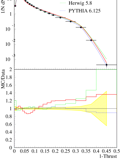
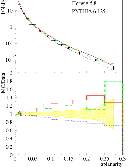
Figure 3: Agreement between various Monte Carlo generators and Delphi event shape distributions. The upper part of the plot shows the observable, the lower one the ratio of Monte Carlo and data; the shaded band represents the error of the data.

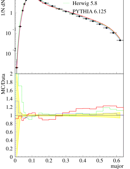
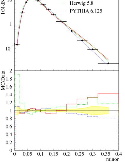
Figure 4: Agreement between various Monte Carlo generators and Delphi event shape distributions. The upper part of the plot shows the observable, the lower one the ratio of Monte Carlo and data; the shaded band represents the error of the data.

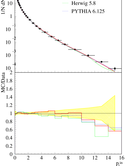
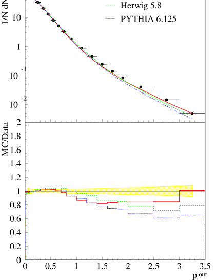
Figure 5: Agreement between various Monte Carlo generators and Delphi inclusive particle spectra. The upper part of the plot shows the observable, the lower one the ratio of Monte Carlo and data; the shaded band represents the error of the data.

Figure 6: Agreement between various Monte Carlo generators and Delphi inclusive particle spectra. The upper part of the plot shows the observable, the lower one the ratio of Monte Carlo and data; the shaded band represents the error of the data.

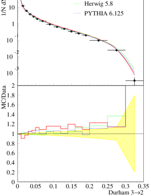
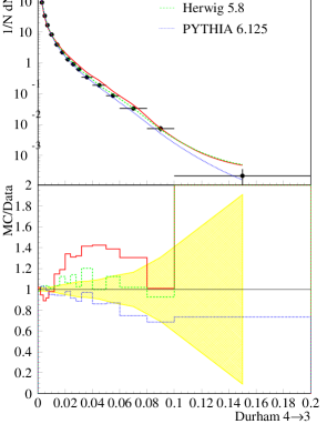
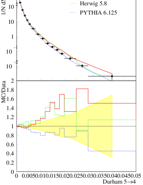
Figure 7: Agreement between various Monte Carlo generators and Delphi jet rates. The upper part of the plot shows the observable, the lower one the ratio of Monte Carlo and data; the shaded band represents the error of the data.

2.5.7 Conclusion and outlook

Apacic++  parameters have been tuned to various sets of Delphi event shape distributions, jet rates and inclusive particle spectra.

The fits converged, the tuned parameters came out to be basically reasonable: The parameter $y_{cut}^{ini}$ has been fixed in the latest tuning. The parameter for the cutoff of the parton shower is high, giving large weight to the fragmentation and minor to the parton shower. This has to be investigated.

Apacic++ is able to predict all examined observables reasonably well. Still none of the examined Monte Carlo generators is able to predict the tail of the $p_{t}^{out}$ distribution (see however Sec. 3.2).

3 INCLUSIVE (ALL FLAVOUR) JET RATES

3.1 Tuning issues

During the Lep1 phase a qualitative improvement of the description of the hadronic final state by parton shower fragmentation models has been reached, mainly due to the possibility to precisely tune the models to a vast amount of high quality data [32]. For this task flexible tuning procedures were used allowing interpolation between model responses generated with different parameter settings [43, 41].

The effects on the model response of the individual parameters of the two major aspects of the models – the parton shower and the actual hadronisation phase – turn out to be strongly correlated. This requires one to determine the most important model parameters in global fits to high statistic event shape and inclusive charged particle spectra and to identified particle data. A recent example for such a fit is discussed in [44].

3.2 Model performance and multi-jet rates

It turns out that the string as well as the cluster hadronisation model are able to represent the major features of particle production, especially the identified particle rates, reasonably well. More detailed discussions can be found in [32, 45, 46].

Distributions depending mainly on the parton shower phase of the models are in general very well represented. Especially for most of the event shape distributions, data and models agree within a few percent. There are two important exceptions to this rule:

Figure 8: $p_{t}^{out}$–distribution as measured by Aleph compared to predictions by Ariadne, Jetset and Herwig [44]

Firstly the tail of the transverse momentum distribution of particles out of the event plane is underestimated by about 30% by most models [32, 41]. A possible explanation for this deficiency is that the parton shower models account for part of the angular structure of multi-jet events by tracing the polarization of the emitted gluons (see e.g. [24]) to further splittings. This approximation cannot account for interference effects like a full matrix-element calculation. It should be emphasized, however, that the most recent tuning [44] of the latest version of Herwig shows a remarkable improvement of the $p_{t}^{out}$-description. This distribution (see Figure 8) now seems almost perfectly reproduced.

Figure 9: Jet-rates for the Durham algorithm as measured by Aleph [51]

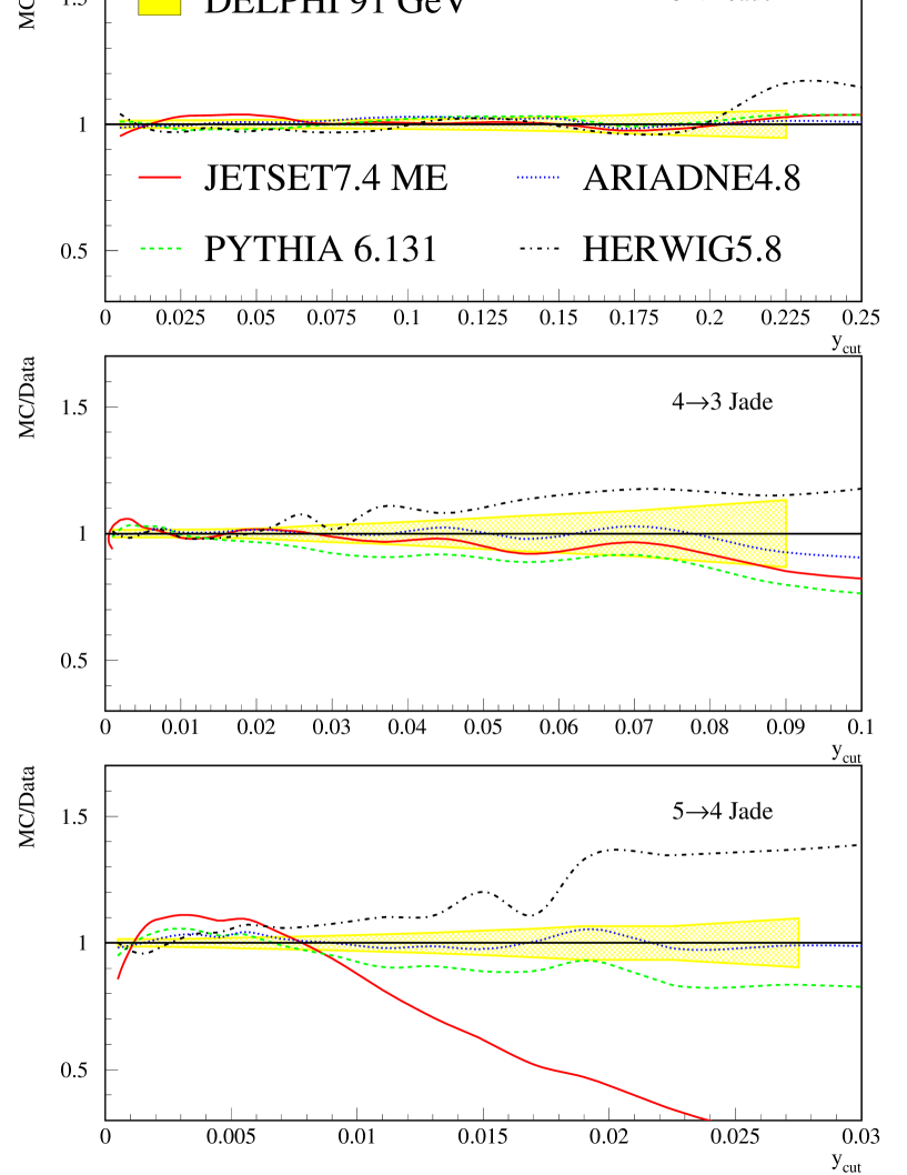
Figure 10: Ratio data/Monte Carlo for the differential 2- (3$\rightarrow$2), 3- (3$\rightarrow$2) and 4 jet (3$\rightarrow$2) rates (Jade algorithm). Data measured by Delphi. The bands represent the statistical errors. Model tunings as in [41]. Jetset ${\cal O}(\alpha_{\mbox{\tiny S}}^{2})$ matrix element option for comparison.

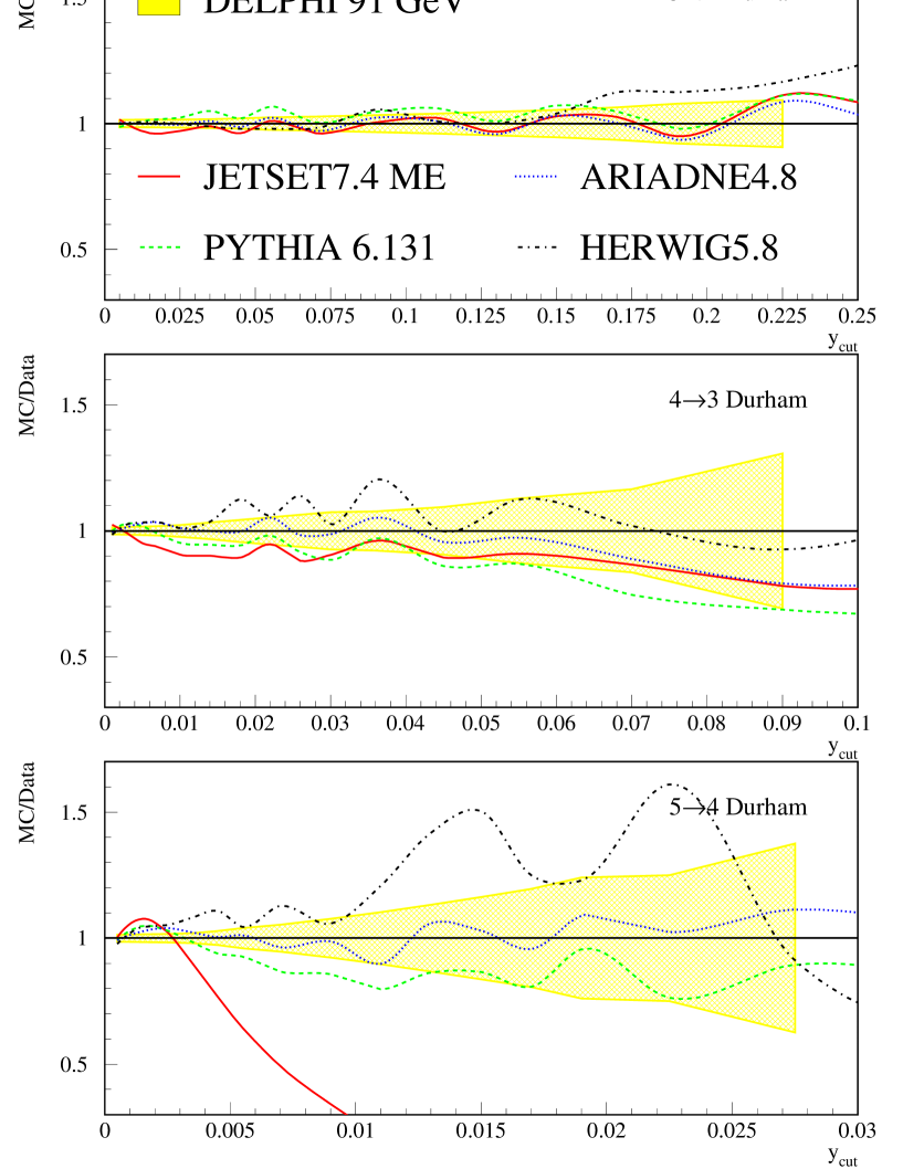
Figure 11: Ratio data/Monte Carlo for the differential 2- (3$\rightarrow$2), 3- (3$\rightarrow$2) and 4 jet (3$\rightarrow$2) rates (Durham algorithm). Data measured by Delphi. The bands represent the statistical errors. Model tunings as in [41]. Jetset ${\cal O}(\alpha_{\mbox{\tiny S}}^{2})$ matrix element option for comparison.

Figure 12: Residuals (data/Monte Carlo -1) for the Cambridge jet algorithm. Data measured by Opal [49]. Error bars depict the experimental errors. Full line: Pythia. Dashed: Herwig. Dotted: Ariadne. Dot-dashed: COJETS [50].

The second exception concerns the inability of Herwig and Pythia/Jetset to simultaneously describe different multi-jet rates with the precision desired by the experiments. This can already be seen from the $y_{cut}$ dependence of the multi-jet rates shown in Figure 9 but is more clearly evident from the direct data/model comparisons in Figures 10, 11 and 12. For a well represented three-jet rate, as was perhaps required in the tunings of the Delphi Collaboration [41], the (differential) four and more jet-rates are systematically overestimated (underestimated) by Herwig or Pythia/Jetset, respectively. This is already observed for the four-jet rate, which is of special importance at Lep2, but is even more so for the five-jet rate. This general trend remains valid even for the aforementioned latest version/tune of Herwig [47]. Depending on the strategy followed by the experiments, this misrepresentation can be distributed differently among the individual jet-rates. For example, the Opal tuning mediates between the rates (see Figure 12). The general discrepancy between multi-jet-rate data and the corresponding model predictions has been reported during the workshop by all experiments.

Only Ariadne so far is able to well represent all jet-rates simultaneously (see Figures 10, 11 and 12). The likely explanation for this difference between Ariadne and the other models lies in the matching between the parton shower and the first order $\rm q\bar{q}g$ matrix element simulations performed in Pythia and Herwig in order to well represent the initial hard gluon radiation. This matching is not needed in the dipole model implemented in Ariadne as here the splitting probability for all splittings is given by the lowest order matrix element expression. The “opposite” behavior observed for Pythia and Herwig may indicate, however, that a better agreement may be reachable by suitably improving the matching procedure.

3.3 Residual uncertainties

Residual uncertainties due to the imperfect description of multi-jet rates are difficult to review globally as they will depend critically on the individual analyses as well as on the tuning chosen by the different experiments.

An incorrect 4-jet rate at high energies may require a reweighting of the Monte Carlo to properly account for the QCD background in W or Higgs analyses. Due to the correlation of the number of jets of an event with other properties, e.g. the charged multiplicity or the momentum spectrum, this is likely to have unwanted side effects. An incorrect value of the strong coupling (which in the tunings is often fixed by the 3-jet rate) may cause an incorrect energy extrapolation of the models which is hard to control at high energy because of the limited data statistics.

A possible strategy for a determination of systematic error for a QCD type observable such as the four jet rate at Lep2 energies may be the following: The quality of the description of the observable is checked at the Z⁰. A possible misrepresentation at the Z⁰ and at high energy is corrected using the same correction factor. A large fraction of the deviation of the correction factor from unity has to be taken as systematic uncertainty of the correction factor at high energy, since the reason for the bad data description, and consequently a possible energy dependence, is unknown.

The additional error for the uncertainty of the energy evolution of the model will in general be small. In the case of the four-jet cross section at high $y_{c}$, it will be dominated by the uncertainty of the strong coupling. From the expected QCD evolution of the four-jet rate [48] this uncertainty is at $\sqrt{s}=200$ GeV:

$$\frac{\delta R_{4}(\sqrt{s})}{R_{4}(M_{\mathrm{Z}})}=4b\ln\left(\frac{\sqrt{s}}{M_{\mathrm{Z}}}\right)\delta\alpha_{\mbox{\tiny S}}(M_{\mathrm{Z}})\simeq 1.9\,\delta\alpha_{\mbox{\tiny S}}(M_{\mathrm{Z}})$$

Here $b=(33-2n_{f})/12\pi\simeq 0.61$. For an optimistically reachable error of $\alpha_{\mbox{\tiny S}}$ in the models of $\delta\alpha_{\mbox{\tiny S}}(M_{\mathrm{Z}})=0.003$ this yields $0.6\%$.

Employing alternative models and alternative model tunings will provide an important cross check of the above error estimate. A model which correctly represents the four-jet cross section at the Z⁰, but overestimates the three-jet cross section ($\propto\alpha_{\mbox{\tiny S}}$) by about 10% (compare Figure 9 at $y_{cut}\sim 0.01~{}{\rm to}~{}0.02$) may in fact lead to a more optimistic error estimate. The error for the correction factor will vanish in this case at the expense of an increased error of the model extrapolation. This error, however, is still small ($1.9\,\delta\alpha_{\mbox{\tiny S}}=1.9\times 0.012\sim 2\%$).

For some analyses already today the abovementioned deficiency of the multi-jet description of the models leads to important contributions to the systematic error. An example is the Delphi measurement of the W pair production cross section with a fully hadronic final state. A systematic error of 5% (including a possible misrepresentation of the jet angular distributions) is here assigned to the major background of QCD events. This error was estimated by comparing different (uncorrected) models and dominates the overall systematics. With increasing statistics this systematic error will be of similar size to the statistical error. Delphi therefore starts to employ Ariadne  which certainly in terms of the jet rates provides the best description of the data, as an alternative model for the full simulation.

4 STUDY OF MASS EFFECTS IN 3- AND 4-JET RATES

4.1 Introduction

The aim of this Section is to study the theoretical precision in the modeling of the rate of QCD processes leading to 3 and 4 final state jets, at Lep1 and Lep2, and involving $b$ quarks. This is important both to help understanding how to treat mass effects in our phenomenological QCD models, and to ensure precise enough control of backgrounds to new particle searches with $b$ quarks in the final state, such as for instance the Higgs search. With this aim in mind we compare mass effects on jet rates in the different MC approaches both to data and to analytic calculations.

It is natural to consider that because of their higher mass, $b$ quarks must from kinematics radiate fewer gluons than light quarks. More generally such a suppression enters in what is often refered to as the dead cone effect. What we want to know is how well the magnitude of this suppression is modeled in our Monte-Carlo approaches, and what is the related theoretical uncertainty. In some sense this question can also be formulated as that of specifying the appropriate mass which should be used for the $b$ quark.

From basic kinematics arguments, it can be shown that the magnitude of the suppression of gluon radiation from mass effects should scale as $m_{b}^{2}/(s.y)$, where $m_{b},s$ and $y$ are the $b$ quark mass, the collision energy squared and jet resolution parameter, respectively. From this scaling law can be anticipated that the effects on jet rates are reduced at Lep2 energies as compared to Lep1, but that they can still remain substantial if jets are defined with a very small $y$ parameter.

In practice, from the results obtained, we find that the above scaling law is very approximate, and can really only be used to give a rough indication of the magnitude of effects. In addition to the purely kinematic effects, resulting from the more limited phase-space, significant corrections - often referred to as dynamic mass effects - arise when taking into account properly the $b$ quark mass in the matrix elements for 3 or 4 final state partons. Moreover, when comparing the data to the behaviour of the analytic calculations or to that of the MC, one must be careful to appropriately take into account in a consistent way effects resulting in final state jets with $b$ quarks other than the radiation of gluons off $b$ quarks, such as processes with a gluon splitting into $b{\bar{b}}$.

In what follows, we first describe the method used for the evaluation. This involves describing briefly the experimental analysis and the procedure enabling meaningful comparisons with analytic calculations and with predictions from Monte-Carlo generators. We then describe the analytic calculations which are available, show how these can be parametrised as a function of $m_{b},s$ and $y$ to enable the above mentioned comparisons, as well as extrapolations. A proposed definition for the theoretical uncertainty to be quoted is also presented and discussed. Then follows a Section presenting the results of the comparisons of the different Monte-Carlo approaches studied (Ariadne, Pythia, Herwig and Fourjphact) with the analytic calculations and with the Delphi data (some of which is still preliminary). The comparisons with data are performed using the high statistics data available from Delphi at Lep1. Several of the used Monte-Carlo programs provide different options for the treatment of mass effects. Also, some have recently benefited from improvements. The main features of the different results and behaviours are described. Finally, remaining issues are discussed. One of these concerns the contribution to the observables used in the evaluation from processes involving gluon splitting into $b{\bar{b}}$. A quantitative measure of the precision of the description provided by the different programs for the 3 and 4 jet cases as a function of $y$, at both Lep1 and Lep2 energies, is given.

4.2 Procedure used for evaluation

4.2.1 Appropriate choice of experimental observable

Any observable with an explicit mass dependence can be computed either using the quark pole mass ($M_{q}$) or the running mass ($m_{q}(\mu)$). Both methods are equally valid, and the results have to be the same if computed to all orders in perturbation theory. However at any fixed finite order the predictions using both schemes do not necessarily agree. At a fixed order, calculations have a dependence on the scale at which the observable is computed. This dependence reveals the size of the higher order terms, as the sum of all the series must have no dependence on the scale.

Aleph [80] has performed a study of the $b$ mass effects on several event shape observables comparing their Leading Order (LO) and NLO terms and hadronization effects. Some observables have quite large mass dependence as shown in that study. However as the raw measurements have to be corrected accounting for the hadronization effects, it so happens that some observables have a correction even larger than the size of the effect to be measured.

Therefore the ideal observable to study quark mass effects will exhibit a large mass dependence, low higher-order corrections and small hadronization effects.

4.2.2 $b$ quark mass effects on the 3-jet ratio

In order to study the $b$ mass effects, both Aleph [80] and Delphi [81, 82] have chosen an observable which fully complies with the above requirements. The observable is the following:

$$R_{3}^{b{\ell}}(y_{c})=\frac{R^{b}_{3}(y_{c})}{R^{\ell}_{3}(y_{c})}$$ (36)

where $R^{b}_{3}(y_{c})$ and $R^{\ell}_{3}(y_{c})$ are the $b$-quark and light-quark 3-jet rates as defined in Eq. 2.

4.2.3 Data analysis

The jets of the hadronic events can be reconstructed by means of a jet finding algorithm (e.g. Durham or Cambridge – see Sec. 1.2). By choosing the appropriate jet resolution parameter $y$, it is possible to force the reconstruction of just three jets in every event. Then, a set of quality cuts are applied over each jet (e.g. minimum charged multiplicity, enough visible energy, …).

4.2.4 Flavour definition

The criterion adopted in [81] and [83] is such that the flavour of the event is defined as that of the quark coupled to the $Z$ in the $Z\rightarrow q\bar{q}$ vertex. By convention, the production of $b$ quarks via the splitting of a bremsstrahlung gluon is ignored in this definition. It was shown that for this particular 3-jet observable, the corresponding effect is practically negligible. As will be seen in Sec. 4.4.4, this is no longer the case in the case of 4-jets.

4.2.5 Flavour tagging technique

The sample of hadronic events is split in two categories, with both events strongly enriched in $b\bar{b}$, by using $b$-tagging, and events strongly enriched in light quarks, by using $anti-b$-tagging.

The tagging procedure normally uses the impact parameter information of all charged particles in the event. Lep experiments are equipped with silicon vertex detectors allowing accurate track reconstruction. $b\bar{b}$ events can be selected by considering the presence of particles with large impact parameter significance (impact parameter over its error), while $\ell\bar{\ell}$ events can be tagged just by the lack of those tracks. In addition the presence or absence of a reconstructed secondary vertex can be used in the $b$-tagging criterion.

4.2.6 Measuring and correcting $R_{3}^{b\ell}$

The measured value of our observable can be computed from the ratio of the reconstructed three-jet rates for $b$ and light quark tagged flavours ($R^{\rm obs}_{3q}(y_{\rm c}),q=b,\ell$):

$$R^{b\ell\rm-obs}_{3}(y_{\rm c})=R^{\rm obs}_{3b}(y_{\rm c})/R^{\rm obs}_{3\ell}(y_{\rm c})$$

This raw value of the observable must be converted into a parton level one which may be compared with the LO and NLO calculations [83, 84]. The correction method accounts for the detector effects, biases introduced in the flavour tagging, and hadronization effects.

The contribution of each flavour, $R^{i}_{3q}$, to the observed three-jet cross section is given by:

$$R^{\rm obs}_{3q}=c^{b}_{q}\cdot R^{b}_{3q}+c^{c}_{q}\cdot R^{c}_{3q}+c^{\ell}_{q}\cdot R^{\ell}_{3q}$$

where $c^{i}_{q}$ represents the flavour content for $i=b,~{}c,~{}\ell$ in each of the experimentally tagged samples.

The reconstruction level and parton level three-jet rates for each flavour and defined sample ($R^{i}_{3q}$ and $R^{\rm par}_{3q}$, respectively) are related by:

$$R^{i}_{3q}(y_{\rm c})=d^{i}_{3q}(y_{\rm c})\cdot h_{3i}(y_{\rm c})\cdot R^{\rm par}_{3i}(y_{\rm c})$$

where $d^{i}_{3q}$ and $h_{3i}$ are correction factors, accounting, respectively, for detector acceptance and tagging effects (deduced from the modeling of the detectors response to hadronic events), and for hadronization effects (estimated by comparing the hadron and parton level distributions obtained from MC programs).

By taking the jet rates from $c$ quarks equal to those from light quarks ($R^{\rm par}_{3c}\equiv R^{\rm par}_{3\ell}$), the measured jet rates can be expressed as:

$$R^{\rm obs}_{3b}(y_{\rm c})=A_{b}(y_{\rm c})\cdot R_{3b}^{\rm par}(y_{\rm c})+B_{b}(y_{\rm c})\cdot R_{3\ell}^{\rm par}(y_{\rm c})$$

$$R^{\rm obs}_{3\ell}(y_{\rm c})=A_{\ell}(y_{\rm c})\cdot R_{3b}^{\rm par}(y_{\rm c})+B_{\ell}(y_{\rm c})\cdot R_{3\ell}^{\rm par}(y_{\rm c})$$

where $A_{q}$ and $B_{q}$ are a redefinition of the original set of parameters: $c^{i}_{q},~{}d^{i}_{3q}$ and $h_{3i}$. This parametrization allows expressing the corrected observable as:

$$R_{3}^{b\ell}(y_{\rm c})=\frac{R_{3b}^{\rm par}}{R_{3\ell}^{\rm par}}=\frac{B_{b}-B_{\ell}\cdot R_{3}^{b\ell{\rm-obs}}}{A_{\ell}\cdot R_{3}^{b\ell{\rm-obs}}-A_{b}}$$

The results are described in Sec. 4.4. At $\sqrt{s}=M_{\mathrm{Z}}$ the total correction to the raw $R_{3}^{b\ell}$ is typically about 10%, the bulk of which corresponds to the detector and tagging effects, while hadronization corrections are of the order of 1%.

Uncertainties in the detector modeling were studied. The main uncertainty results from the limited statistics of fully simulated events with detector response, resulting in limited knowledge of the factors $c^{i}_{q}$ describing the flavour content of each of the tagged samples. This error was estimated to be roughly 0.3%, but has a strong dependence on the jet resolution parameter $y_{c}$ as it is directly related to the statistics of the three-jet simulated sample. Uncertainties from the modeling of the hadronization were also studied, and are described in Sec. 4.5.

4.2.7 $b$ quark mass effects on the 4-jet ratio

The study of the $b$ quark mass in the 4-jet rate was performed by Delphi in [82]. The analysis uses an observable defined in a similar manner to $R_{3}^{b\ell}$:

$$R_{4}^{b{\ell}}(y_{c})=\frac{R^{b}_{4}(y_{c})}{R^{\ell}_{4}(y_{c})}$$ (37)

where $R^{b}_{4}(y_{c})$ and $R^{\ell}_{4}(y_{c})$ are the $b$-quark and light-quark 4-jet rates as defined in Eq. 2.

The analysis was similar to the $R_{3}^{b\ell}$ and also reveals a clear dependence of the 4-jet rate on the quark mass. However $R_{4}^{b\ell}$ has only been computed at LO level (see Sec. 4.3). The result of the analysis are shown in Sec. 4.4.

4.3 Analytical calculations

The next-to-leading order (NLO) matrix element (ME) calculation for the process $e^{+}e^{-}\rightarrow 3$ jets, with complete quark mass effects, has been performed independently by three groups [83, 84, 85]. These predictions are in agreement with each other and were successfully used in the measurements of the bottom quark mass far above threshold [86, 87, 82, 80] and in the precision tests of the universality of the strong interaction [86, 88, 89] at the $Z$-pole. Instead, only leading order (LO) predictions for 4-jet final states with heavy quarks are available [17, 18] at present.

In this Section we discuss in detail the ME calculation for the process $e^{+}e^{-}\rightarrow 4$ jets with quark mass corrections. A procedure to estimate the theoretical uncertainty of the LO calculation, i.e. of the expected higher order corrections, is also described. First, we present and test this procedure in the 3-jet case, where the recent available NLO corrections can be compared with the LO calculation. Then, these results are extrapolated to the 4-jet case for which the higher order corrections are estimated.

Since quarks are not free particles it seems natural to treat their mass like a coupling constant. In other words, we can work with quark masses defined in several renormalization schemes. As was already pointed out in Sec. 4.2.1, the physical result cannot depend on which mass definition is used in the ME calculation, but if at a fixed order in perturbation theory the ME calculation gives different results for different quark mass definitions, this difference should come from higher order corrections. Therefore, at a given order, the spread of the results for different mass definitions can be taken as an estimate of the theoretical uncertainty of the calculation, i.e. as an estimate of higher order corrections.

In the following we consider the ME calculation for the production of bottom quarks through the processes $e^{+}e^{-}\rightarrow$ 3-jets, 4-jets in two different schemes: the perturbative pole scheme and the running scheme. In the former, the calculation is performed with the perturbative pole mass $M_{b}\sim 5$ GeV. In the later, we use the $\overline{MS}$ scheme running mass $m_{b}(\mu)$, normalized at the center of mass energy of the collision, $m_{b}(M_{\mathrm{Z}})\sim 3$ GeV at Lep1 energies. The two results define a band which can be taken as an estimate of the higher order corrections.

At the NLO the bottom quark 3-jet cross section receives contributions from one-loop corrected three parton final states, $e^{+}e^{-}\rightarrow Z,\gamma^{*}\rightarrow b\bar{b}g$, and tree level four parton final states, $e^{+}e^{-}\rightarrow Z,\gamma^{*}\rightarrow b\bar{b}gg,b\bar{b}b\bar{b},b\bar{b}q\bar{q}$, with $q\neq b$. These contributions can be handled and classified through the different cuts to the bubble diagrams of Figure 13 giving rise to three and four parton final states.

Figure 13: Feynman diagrams relevant for the processes $e^{+}e^{-}\rightarrow$ 3-jets, 4-jets.

We first evaluate the ratio of three-jet rates defined by Eq. 36, which can be interpreted as the measure of the suppression of gluon radiation off $b$-quarks with respect to gluon radiation off light quarks, $\ell=u,d,s$.In this ratio, most of the electroweak corrections cancel out.

In Figure 14, the $R_{3}^{b\ell}$ observable is presented at NLO for the Durham and the Cambridge algorithms at the $Z$-peak energies, $\sqrt{s}=M_{\mathrm{Z}}$, in the running mass (NLO-$m_{b}(M_{\mathrm{Z}})$) and the pole mass (NLO-$M_{b}$) schemes. For comparison, the LO results – LO-$m_{b}(M_{\mathrm{Z}})$ and LO-$M_{b}$ – are also plotted. At a fixed order, the band defined by the results in both schemes is taken as our estimate of the theoretical uncertainty of the calculation at this order. As one would naturally expect, the width of this band is reduced at the NLO with respect to the LO result, roughly by a factor two in Durham or even more in Cambridge. Furthermore, we found that the two LO predictions bound the NLO results in both algorithms. This suggests that higher order contributions cannot be too large and may be bounded by the lower order results.

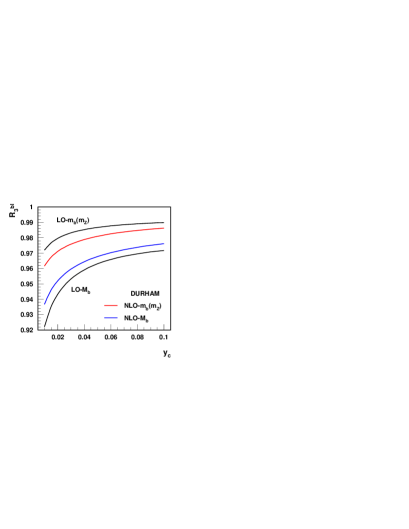
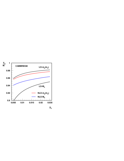
Figure 14: The observable $R_{3}^{b\ell}$ as a function of $y_{c}$ at NLO for the Durham and Cambridge jet-algorithms at the center of mass energy $\sqrt{s}=M_{\mathrm{Z}}$. The blue (lower inner) lines give the observable computed at the NLO in terms of the pole mass $M_{b}=5$ GeV. The red (upper inner) lines show the result for a running mass $m_{b}(M_{\mathrm{Z}})=3$ GeV. In both cases the renormalization scale is fixed to $\mu=M_{\mathrm{Z}}$, with $\alpha_{\mbox{\tiny S}}(M_{\mathrm{Z}})=0.118$. For comparison we also plot in solid lines the LO results for $M_{b}=5$ GeV (LO-$M_{b}$) and $m_{b}(M_{\mathrm{Z}})=3$ GeV (LO-$m_{b}(M_{\mathrm{Z}})$).

Next we consider the process $e^{+}e^{-}\rightarrow 4$ jets. The ratio of four-jet rates is defined in Eq. 37. At LO, only four parton final state cuts to the bubble diagrams of Figure 13 have to be considered. Let’s interpret for the moment, $R_{4}^{b\ell}$ as the suppression of gluon radiation from primary $b$-quarks in four-jet events. By primary quarks we mean that the flavour of an event is defined by the flavour of the quark directly coupled to the $Z$ or $\gamma^{*}$ bosons. This implies that events where a bottom-antibottom pair is produced from gluon radiation off a light quark pair (the so-called gluon splitting into $b{\bar{b}}$) are considered as light events, even though they actually involve $b$ quarks, and their contribution is added to the denominator of Eq. 37). In $R_{3}^{b\ell}$, the contribution from gluon splitting into $b{\bar{b}}$ was calculated to be small, resulting in effects of the order of a few permil. This is not the case for four-jet events, where larger contributions can justify, as will be explained in Sec. 4.4.4, the consideration of a different convention for the jet rate ratio defined above, in which the numerator receives contributions from all events involving $b$-quarks.

At LO and for the definition with the primary quark convention, the $R_{4}^{b\ell}$ ratio can be parameterized in the following way

$$R_{4}^{b\ell}=1+\frac{m_{b}^{2}}{s}\left[\sigma_{V}(s)H_{V}\left(\frac{m_{b}^{2}}{s},y_{c}\right)+\sigma_{A}(s)H_{A}\left(\frac{m_{b}^{2}}{s},y_{c}\right)\right]~{},$$ (38)

were $m_{b}$ can be either the pole mass, $M_{b}$, or the running mass at some renormalization scale, $m_{b}(\mu)$, typically $\mu=\sqrt{s}$, of the bottom quark, $\sigma_{V,A}$ is a function of the vector (axial-vector) couplings of the quarks to the $Z$-boson and the photon, and $H_{V,A}$ gives the behaviour as a function of the resolution parameter $y_{c}$, and can also contain a small residual dependence on the ratio $m_{b}^{2}/s$.

In Figure 15, the $R_{4}^{b\ell}$ ratio is shown at LO in the Durham algorithm at the center of mass energies $\sqrt{s}=M_{\mathrm{Z}}$ and $\sqrt{s}=189$ GeV. For the same center of mass energy, the suppression of gluon radiation from $b$-quarks is a larger effect in four-jet events than in three-jet events. At $\sqrt{s}=M_{\mathrm{Z}}$, it amounts to roughly $10\%$, which also corresponds to the difference between the two LO predictions, LO-$m_{b}(M_{\mathrm{Z}})$ and LO-$M_{b}$, taken as the theoretical uncertainty of the LO prediction. If the behaviour for three-jet events really could be extrapolated to the four-jet case, we would expect that this difference be reduced hopefully by half, if the still uncalculated NLO corrections were included. At $\sqrt{s}=189$ GeV, we get a plot that is roughly scaled by a factor $4$ with respect to the result at the Lep1 energies. But even in this case, the theoretical uncertainty, i.e. the difference between the two LO predictions, can be as large as $5\%$ for small values of the jet resolution parameter $y_{c}$.

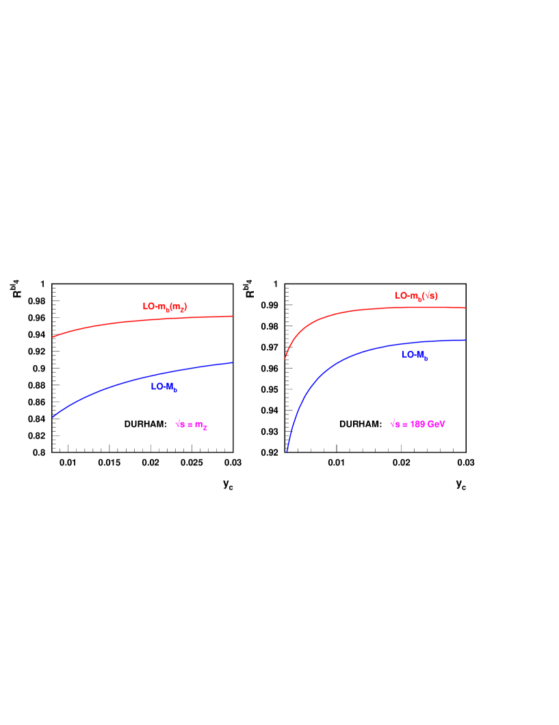
Figure 15: The observable $R_{4}^{b\ell}$ as a function of $y_{c}$ at LO in the Durham algorithm for $\sqrt{s}=M_{\mathrm{Z}}$ and $\sqrt{s}=189$ GeV.

4.4 Comparisons for $R_{3}^{b\ell}$ and $R_{4}^{b\ell}$ at LEP1 and LEP2

Following the procedure described above, we compare at both Lep1 and Lep2 energies, the double jet rate ratios $R_{3}^{b\ell}$ and $R_{4}^{b\ell}$ obtained with the different Monte-Carlo approaches studied (Ariadne, Pythia, Herwig and Fourjphact) with the analytic calculations, and, in the case of Lep1, with the data. All these comparisons are done at the level of partons (hadronization and non-perturbative effects are considered in Sec. 4.5). In Figures 16,  17 and  18 are indicated both the LO matrix element results for $m_{b}=$ 3 and 5 GeV and the NLO results for $m_{b}=$ 3 GeV, in the case of the 3-jet rates at Lep1. In Figures 19,  20,  21 and  22 are indicated only the LO results for $m_{b}=$ 3 and 5 GeV for the 4-jet rates at Lep1. In Figures 23,  24 and  25 are indicated the LO results for $m_{b}=$ 3 and 5 GeV for the 4-jet rates at Lep2. The band defined by the pair of LO curves is in each case taken, conservatively, to represent the theoretical uncertainty in the ratios $R_{3}^{b\ell}$ and $R_{4}^{b\ell}$, as was explained in Sec. 4.3.

4.4.1 Three jet rates at $\sqrt{s}=M_{\mathrm{Z}}$

In Figures 16,  17 and  18 are shown the comparisons for $R_{3}^{b\ell}$ at $\sqrt{s}=M_{\mathrm{Z}}$ between the analytic calculations, the data[81, 82] and the Monte-Carlo generators Pythia, Herwig, Ariadne and Apacic++, respectively.

The Pythia comparison in Figure 16 shows three curves corresponding to:

• The initial treatment, with mass effects only present in the limitation of the phase-space available in $b\rightarrow bg$ branchings in the parton shower, but not in the kinematics of these branchings, and with massless matrix elements used in the matching procedure applied to the 3 jets generated (Jetset versions $\leq$ 7.3, or any present version with the switch MSTJ(47) set to 1 to turn off subsequent additional mass effects).

• Mass effects present in the limitation of the phase-space available in $b\rightarrow bg$ branchings in the parton shower, but not in the kinematics of these branchings, and with massive matrix elements used in the matching procedure applied to the 3 jets generated (Pythia versions 5.7-6.125).

• Mass effects present in the limitation of the phase-space available in $b\rightarrow bg$ branchings in the parton shower, in the kinematics of these branchings, and with massive matrix elements used in the matching procedure applied to the 3 jets generated (Pythia versions $\geq$ 6.130).

As can be seen the recent changes consisting in introducing mass effects at all stages in the treatment (see Sec. 2.1.1) result in a very good behaviour. In the prior versions which are presently still used by a majority of Lep experiments, a behaviour almost as good is obtained by using massless expressions for the matching procedure of the generated 3 jets (switch MSTJ(47) set to 1).

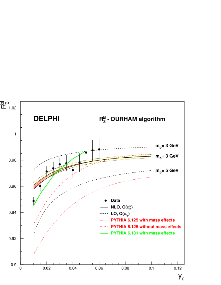
Figure 16: $R_{3}^{b\ell}$ double ratios at $\sqrt{s}=M_{\mathrm{Z}}$ for Pythia 6.125, with mass switch on and off, and for Pythia 6.131, with mass switch on

The Herwig comparison in Figure 17 shows a single curves corresponding to the massive options. A reasonable description is evident, even if the predicted rate is slightly lower than the data and NLO result.

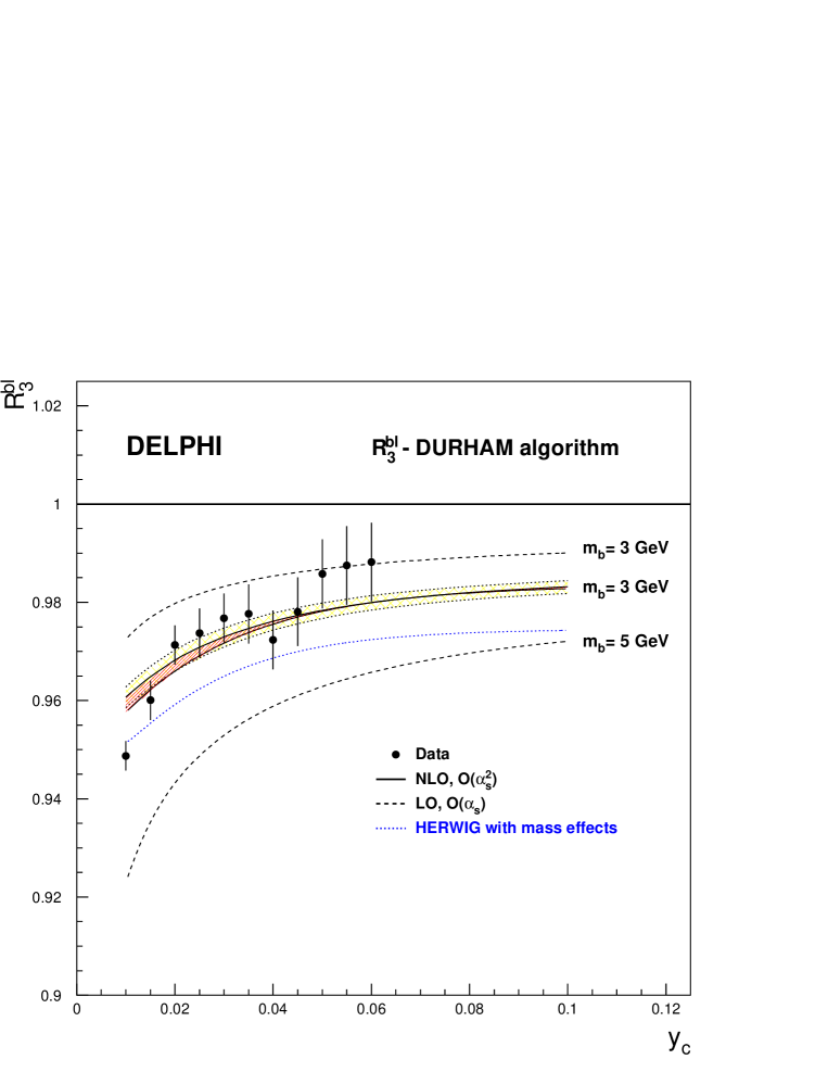
Figure 17: $R_{3}^{b\ell}$ double ratios at $\sqrt{s}=M_{\mathrm{Z}}$ for Herwig 5.8, with mass effects on.

The Ariadne comparison in Figure 18 shows three curves corresponding to using the optional extra dead cone suppression available (MSTA(19)=1), and to the new treatment of heavy masses described in Sec. 2.3.1, in which the full leading order massive matrix element was introduced to describe the branching of the first gluon emitted in $q{\bar{q}}$ events. As can be seen the rate is too low when no optional extra dead cone suppression is used, and then gets even worse when it is used. The new treatment of heavy masses is a clear improvement compared to the old treatment with the dead cone suppression option turned on. But the best behaviour is still achieved when no mass corrections are used.

Figure 18: $R_{3}^{b\ell}$ double ratios at $\sqrt{s}=M_{\mathrm{Z}}$ for Ariadne 4.08, with dead cone switch on and off, and with the new mass treatment described in Sec. 2.3.1.

4.4.2 Four jet rates at $\sqrt{s}=M_{\mathrm{Z}}$

The Pythia comparison in Figure 19 shows three curves corresponding to the three cases described above. As can be seen the recent changes consisting in introducing mass effects at all stages in the treatment also improve the description, as for the three jet case, but still results in a rate which is too low by about 5-7% with respect to data and to the LO matrix element predictions. The same trend is seen as for the three jet case that in the prior versions still presently used by a majority of Lep experiments, the best behaviour is obtained by using massless expressions for the matching procedure of the generated 3 jets (switch MSTJ(47) set to 1).

Figure 19: $R_{4}^{b\ell}$ double ratios at $\sqrt{s}=M_{\mathrm{Z}}$ for Pythia 6.125, with mass switch on and off, and for Pythia 6.131, with mass switch on.

The Herwig comparison is shown in Figure 20. A description compatible with the data and with the LO matrix element prediction can be seen.

Figure 20: $R_{4}^{b\ell}$ double ratios at $\sqrt{s}=M_{\mathrm{Z}}$ for Herwig 5.8, with mass effects on.

The Ariadne comparison in Figure 21 shows three curves corresponding to using the optional extra dead cone suppression available (MSTA(19)=1), and to the new treatment of heavy masses described in Sec. 2.3.1. As can be seen, contrary to the three jet case, the overall behaviour is quite reasonable when no optional extra dead cone suppression is used, but somewhat too low when it is used. The behaviour with the newly changed treatment of heavy masses does not improve the situation significantly: the best behaviour is still achieved when no mass corrections are used, as in the case of $R_{3}^{b\ell}$.

Figure 21: $R_{4}^{b\ell}$ double ratios at $\sqrt{s}=M_{\mathrm{Z}}$ for Ariadne 4.08, with dead cone switch on and off, and with the new mass treatment described in Sec. 2.3.1.

Finally the result of an initial investigation of $R_{4}^{b\ell}$ with the new Fourjphact program is shown in Figure 22. The LO ME curves calculated within Fourjphact are identical to those shown in Figure 19, Figure 20 and Figure 21. The results after only the subsequent parton shower are also shown, as calculated starting from the LO ME with 4.6 GeV, and indicate as expected an exageration of the suppression of gluon radiation from the $b$ quark mass. Presumably, if a way could be found in this program to start the matching procedure from the LO ME with 2.8 GeV (rather than 4.6 GeV) while preserving the corresponding jet angles, one could perhaps contemplate getting the LO ME + parton shower only results to lie in the middle of the band of uncertainty defined in Sec. 4.3, where the NLO results are expected. The result after both parton shower and hadronisation are also shown, although here it is fair to say that the large effect seen from the hadronisation is not understood and should be studied more.

Figure 22: $R_{4}^{b\ell}$ double ratios at $\sqrt{s}=M_{\mathrm{Z}}$ for Fourjphact, with mass effects on. The full (dashed) line shows the result at parton level only, before any subsequent parton showering (see Sec. 2.1.6), for a $b$ quark mass of 2.8 (4.6) GeV. These curves are equivalent to the LO ME curves in Figure 19. The dotted and dashed dotted lines shows the result after subsequent PS and hadronisation, and after only the subsequent PS, respectively.

4.4.3 Four jet rates at $\sqrt{s}=189$ GeV

The Pythia 4 jet rate comparison was repeated at $\sqrt{s}=189$ GeV. This is shown in Figures 23 and 24. A trend similar to that at $\sqrt{s}=M_{\mathrm{Z}}$ can be seen. For values of the jet resolution parameter in the range $y=0.002-0.008$, even with the most recent treatment consisting in introducing mass effects at all stages in the handling of the three jets, a residual deficit of about 1-3% with respect to the LO matrix element predictions. Also, in the prior versions still presently used by a majority of Lep experiments, the best behaviour is obtained by using massless expressions for the matching procedure of the generated three jets (switch MSTJ(47) set to 1). If the massive treatment is used in these prior versions is used, a deficit as large as about 2-6% results in the range $y=0.002-0.008$ (see Figure 23).

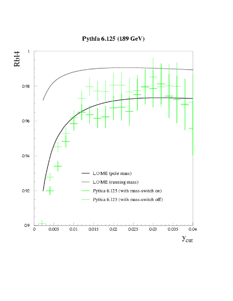
Figure 23: $R_{4}^{b\ell}$ double ratios at 189 GeV for Pythia 6.125, with mass switch on and off

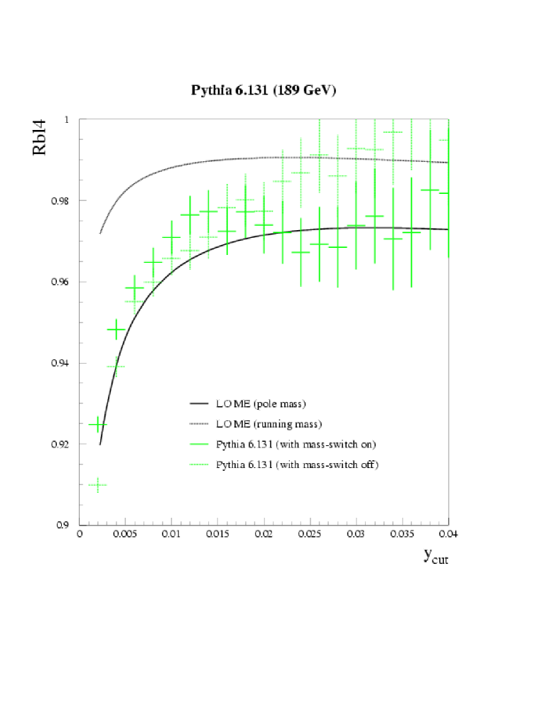
Figure 24: $R_{4}^{b\ell}$ double ratios at 189 GeV for Pythia 6.131, with mass switch on and off

The Ariadne 4.08 4 jet-rate comparison was also repeated at $\sqrt{s}=189$ GeV. This is shown in Figure 25. The same trend is seen as for the 4-jet rate at Lep1 energies: a quite reasonable behaviour is observed when no optional extra dead cone suppression is used, but the rate is somewhat too low when it is used. The behaviour with the recently changed treatment of heavy masses described Sec. 2.3.1 is also shown. As can been the new treatment does not improve the description at Lep2 energies.

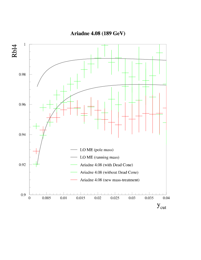
Figure 25: $R_{4}^{b\ell}$ double ratios at 189 GeV for Ariadne 4.08, with dead cone switch on and off, and with the new mass treatment described in Sec. 2.3.1.

4.4.4 Effects of gluon splitting on $R_{4}^{b\ell}$

An additional issue was raised during the meetings of this working group concerning the impact on the evaluation of $R_{4}^{b\ell}$ arising from uncertainties in processes involving gluon splittings into $b{\bar{b}}$. In the case of the three-jet rate ratio $R_{3}^{b\ell}$, the effect was investigated and found to be small. On the contrary, for four jets, because of the lower rate, and because the two $b$ quarks emerging from gluon splittings are often resolved, effects are larger.

The standard definition of $R_{4}^{b\ell}$ presented in Sec. 4.2.7 considers primary quarks, and is advantageous from the theoretical point of view, but not from the experimental one, where such a distinction is obviously not straightforward. Since the data are extrapolated to the parton level using a Monte-Carlo to compare with the calculations, a wrong assumption on the gluon splitting into $b{\bar{b}}$ translates directly into a bias. In order to estimate this bias, a new definition was proposed, labeled $R_{4}^{b\ell}$(NEW) in which are counted in the numerator any event containing $b$ quarks, irrespective whether they originate from primary or secondary production, and at the denominator only events with light quarks, excluding those with a gluon splitting into $b{\bar{b}}$. This new observable is closer to the experimental situation, but is known to carry larger NLO corrections, and is hence more uncertain theoretically. It was nonetheless evaluated both at $\sqrt{s}=M_{\mathrm{Z}}$ and at at $\sqrt{s}=189$ GeV, analytically and using Pythia 6.131, with the different settings corresponding to different recent treatments of the gluon splitting process into $b{\bar{b}}$ developed in the framework of the working group (see Sec. 7.3). As an example the normalised difference $(R_{4}^{b\ell}\mbox{(NEW)}-R_{4}^{b\ell})/R_{4}^{b\ell}$ is shown for $\sqrt{s}=M_{\mathrm{Z}}$ in Figures 26 and 27, respectively for the present default settings (MSTJ(44)=MSTJ(42)=2), and for one of the proposed set of new settings described in Sec. 7.3 (MSTJ(44))=MSTJ(42)=3), corresponding to a $g\rightarrow b\bar{b}$ rate which is roughly doubled. The same comparison is shown for $\sqrt{s}=189$ GeV in Figures 28 and 29.

A general feature of these plots is that at small $y_{c}$ Pythia is always lower. This arises because in Pythia, contrary to the analytic calculation, the four-jet rates in both the denominator and numerator of $R_{4}^{b\ell}$ receive contributions also from two and three jets, which reduce the relative impact from the fraction of events containing a gluon splitting into $b\bar{b}$. Considering firstly the results at $\sqrt{s}=M_{\mathrm{Z}}$, one can see that indeed doubling the gluon splitting rate into $b\bar{b}$ in Pythia results in a difference between the two definitions which at large $y_{c}$ becomes similar to that obtained in the analytical calculation. Since doubling the gluon splitting rate into $b\bar{b}$ tends to be favoured by both experimental results and theoretical work (see Sec. 7.3), one can in principle take this found consistency as evidence confirming that it indeed needs to be doubled in Pythia. To check this further, the fraction of events containing a $g\to b\bar{b}$ splitting in which the two $b$ quarks are clustered into separate jets (case of resolved gluon splittings) was evaluated and found to be largely dominant. This indicated that large NLO corrections in the new definition $R_{4}^{b\ell}$(NEW) are not expected to arise from gluon splittings into $b\bar{b}$, and that most of the effect does occur at LO. From this can be concluded that a procedure consisting in correcting the measured four-jet events in data to extrapolate to the parton level using a Monte-Carlo induces a sensitivity to the correct rate of gluon splittings into $b\bar{b}$, at the level of these discrepancies between the differences. A second conclusion is that indeed at $\sqrt{s}=M_{\mathrm{Z}}$ doubling the rate of gluon splittings into $b\bar{b}$ would seem to be justified from the found consistency of the comparison with the analytical results.

The picture changes however at $\sqrt{s}=189$ GeV. As can be seen from Figure 29, the Pythia curve with doubled gluon splitting into $b\bar{b}$ rate now overshoots significantly at large $y_{c}$ To understand the origin of this behaviour, the same study was performed as at $\sqrt{s}=M_{\mathrm{Z}}$ to evaluate the fraction of events containing a gluon splitting into $b\bar{b}$ in which the gluon splitting is resolved, and it was found that at 189 GeV only about half are. Hence in this case the origin of the overshooting could be traced to the fact that the new definition receives large contributions at NLO from gluon splittings into $b\bar{b}$. Such a behaviour is in fact expected from the scaling with energy of this last contribution, which grows like $\log(m_{b}^{2}/s)$.

None of these results prevent one from evaluating the performance of Monte-Carlo programs using the standard definition for $R_{4}^{b\ell}$. However one must be careful as soon as one wants to compare with data. Moreover, the results at 189 GeV should not be taken as evidence against a larger rate of gluon splittings into $b\bar{b}$ in Pythia, which may be needed as explained in Sec. 7.3, but just that for the case of the observable $R_{4}^{b\ell}$(NEW) the comparison is not meaningful, because of the large NLO contributions affecting it. A full calculation at NLO would be helpful to study this further.

Figure 26: Difference of the $R_{4}^{b\ell}$ double jet ratio at $\sqrt{s}=M_{\mathrm{Z}}$ for Pythia 6.131 (shown with stars) in the NEW and standard definitions, for the default settings with unmodified rate of gluon splitting into $b{\bar{b}}$, corresponding to MSTJ(44)=MSTJ(42)=2, and in the LO matrix element calculation.

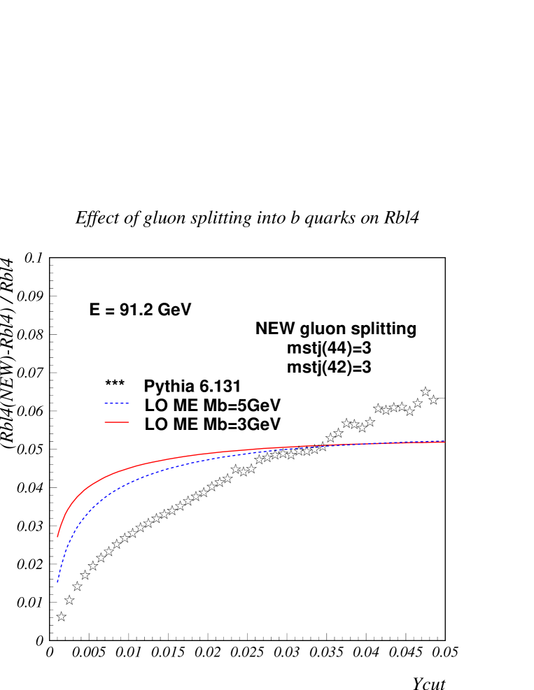
Figure 27: Difference of the $R_{4}^{b\ell}$ double jet ratio at $\sqrt{s}=M_{\mathrm{Z}}$ for Pythia 6.131 (shown with stars) in the NEW and standard definitions, for the settings with increased rate of gluon splitting into $b{\bar{b}}$ corresponding to MSTJ(44)=MSTJ(42)=3, and in the LO matrix element calculation.

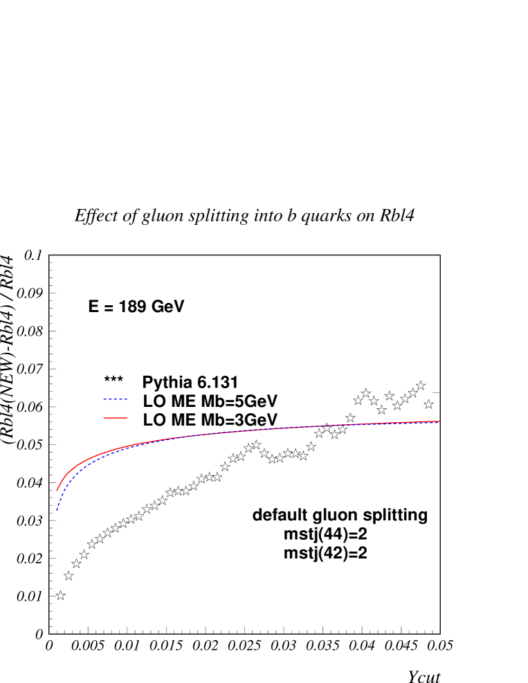
Figure 28: Difference of the $R_{4}^{b\ell}$ double jet ratio at $\sqrt{s}=189$ GeV for Pythia 6.131 (shown with stars) in the NEW and standard definitions, for the default settings with unmodified rate of gluon splitting into $b{\bar{b}}$, corresponding to MSTJ(44)=MSTJ(42)=2, and in the LO matrix element calculation.

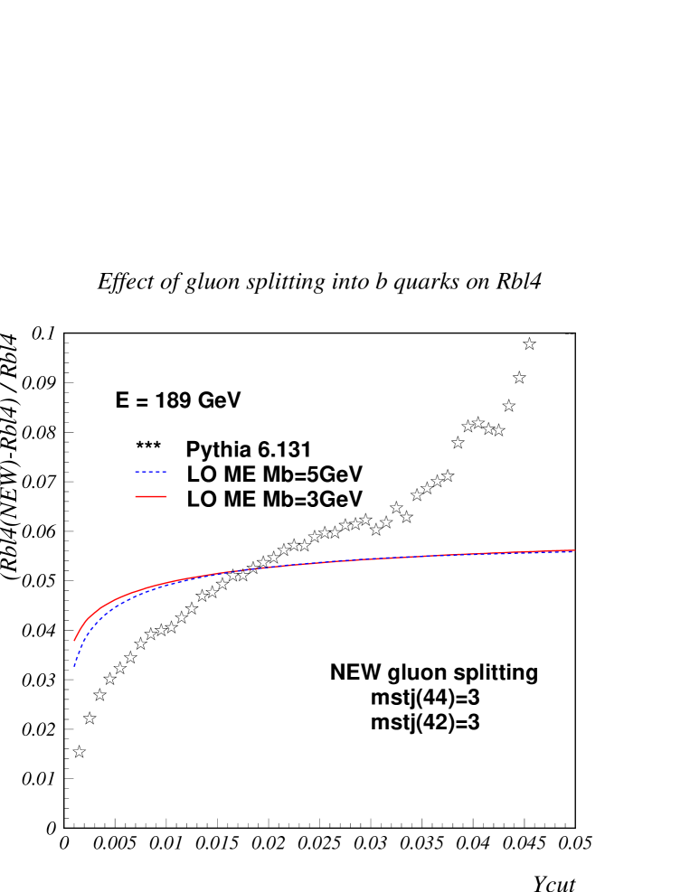
Figure 29: Difference of the $R_{4}^{b\ell}$ double jet ratio at $\sqrt{s}=189$ GeV for Pythia 6.131 (shown with stars) in the NEW and standard definitions, for the settings with increased rate of gluon splitting into $b{\bar{b}}$ corresponding to MSTJ(44)=MSTJ(42)=3, and in the LO matrix element calculation

4.5 Discussion of hadronization corrections to $R_{3}^{b\ell}$

In most of the experimental analyses that involve hadronic final states, the data need to be corrected to the parton level in order to be compared with the theoretical predictions. In particular, this is true for the studies considered in this report, for instance the determination of the $b$-quark mass, or the studies of the flavour independence of the strong coupling constant and the multi-jet production rates. This procedure necessarily implies unfolding the data for detector and acceptance effects as well as for the hadronization process. This introduces biases and uncertainties which need to be carefully studied and quantified to extract reliable measured values within the quoted errors. The detector and acceptance corrections depend on each particular experiment and consequently will not be discussed here. Only the hadronization correction will be the subject of this section. As shown in references [81, 80, 89, 87, 88] the uncertainty arising from the lack of precise knowledge of how the hadronization process takes place limits the experimental precision of the experimental quantities and QCD tests. Any progress leading to a better understanding of the transition from partons to hadrons or finding new observables with better behaved properties will immediately result in improving these measurements.

In particular, let us consider the hadronization corrections associated with the $R_{3}^{b{\ell}}$ observable introduced in Eq. 34 (though on a qualitative basis the same procedure can be easily applied and generalized to the $R_{4}^{b{\ell}}$ observable of Eq. 35 or other event shape variables). This observable summarizes most of the features commented on in previous sections and at the same time has the advantage of being calculated up to NLO (see section 4.3) and of having relatively small fragmentation corrections (of roughly $\sim$1%). The fragmentation models considered in this exercise are Pythia and Herwig. The analysis is also performed using two jet clustering algorithms: Durham and Cambridge, and the potential results of using one or the other are compared and discussed. The determination of $b$-quark mass or the test of the flavour independence of the strong coupling constant can be derived from this observable and the implications are obvious: a better understanding of $R_{3}^{b{\ell}}$ with a smaller error leads to a more precise determination of the $b$-quark mass or a more stringent test of the flavour independence of $\alpha_{\mbox{\tiny S}}$.

In general there is no prescription to unambiguously define the fragmentation correction factor to be applied to the $R_{3}^{b{\ell}}$ observable but the procedure described below can be regarded as a reasonable approach. It is based on the Delphi procedure [81], though others methods could also be envisaged for this purpose [80]. It seems appropiate then to consider all models which give a good description of the data and calculate the correction factor corresponding to each model. The average of the correction factors obtained is taken as the best estimate of the correction factor and the distribution of these values defines the uncertainty. This also means that the models or generators considered in the analysis should be tuned in order to properly describe the data. The overall fragmentation uncertainty can then be quantified by adding in quadrature the two different source of errors: $\sigma_{mod}$, the uncertainty due to the dependence of the hadronization correction factors on the two models considered, Pythia and Herwig, and $\sigma_{tun}$, uncertainty due to the possible variation of the main fragmentation parameters in Pythia. Hence, the total uncertainty is expressed as:

$$\sigma_{had}(y_{c})=\sqrt{\sigma_{mod}^{2}(y_{c})+\sigma_{tun}^{2}(y_{c})}\;.$$ (39)

Following the Delphi procedure the $\sigma_{tun}$ uncertainty is obtained by varying the most relevant parameters of the string fragmentation model incorporated in Pythia ($Q_{0}$, $\sigma_{q}$, $\epsilon_{b}$, a and b) within an interval of $\pm 2\sigma$ from their central tuned values and assuming that the individual parameter errors are all independent. Figure 30 shows, for the Cambridge algorithm, the $\sigma_{tun}$ uncertainty as a function of the jet resolution parameter as well as the contribution of each individual parameter error. For large enough $y_{c}$ values the overall $\sigma_{tun}$ uncertainty is seen to be around 3$0$$\!/$$\!00$. The different tuned versions of Jetset or Pythia have also been tested and cross-checked to give the same correction factors to the observable $R_{3}^{b{\ell}}$ within 1$0$$\!/$$\!00$.

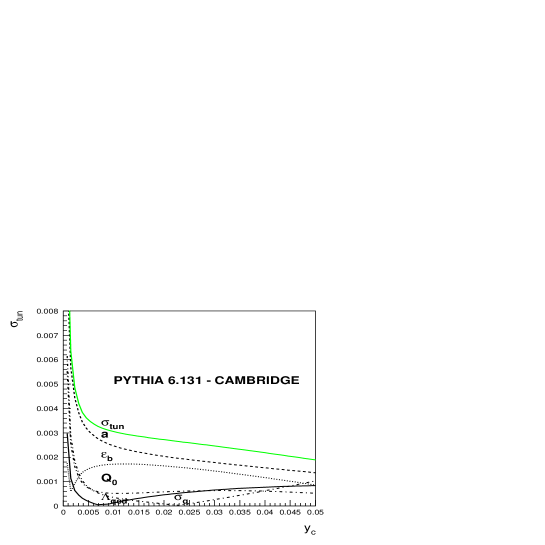
Figure 30: The $\sigma_{tun}$ uncertainty and the contributions of each individual fragmentation parameter considered to the the total error, obtained with the Cambridge algorithm.

In this exercise, the two fragmentation schemes considered are Pythia and Herwig, therefore the average of the two correction factors obtained is considered as the fragmentation correction factor to $R_{3}^{b{\ell}}$ and the uncertainty $\sigma_{mod}$ is taken to be half of their difference. The generators differ not only in the fragmentation process (cluster fragmentation in Herwig and Lund string fragmentation in Pythia) but also in the way the particle decays are implemented. Therefore $\sigma_{mod}$ has two contributions, one from the fragmentation scheme itself, $\sigma_{mod-frag}$, and the other one from the decay tables used, $\sigma_{mod-dec}$, so it can be written as:

$$\sigma_{mod}(y_{c})=\sqrt{\sigma_{mod-frag}^{2}(y_{c})+\sigma_{mod-dec}^{2}(y_{c})}\;.$$ (40)

We present here the results of the $\sigma_{mod}$ uncertainty obtained with Herwig version 5.8 as tuned by Delphi and version 6.1 as tuned by Aleph. For Pythia, the Delphi tuning is used. Presently all Lep  experiments are working on the tuning of new versions, therefore new and better sets are expected soon. Figure 31 shows $\sigma_{mod}$ and $\sigma_{mod-frag}$ at different $y_{c}$ values as calculated using the Durham jet clustering algorithm. For $y_{c}\geq 0.02$ the contribution of $\sigma_{mod-dec}$ to the total model uncertainty becomes small. Also a better agreement between the latest generator versions of Herwig and Pythia is observed over the entire $y_{c}$ region. This result probably is a consequence of the fact that in the latest versions of both generators the $b$-fragmentation functions are now similar. How well these models describe this distribution in data is, however, discussed elsewhere (section 6) and new analyses are still emerging from the various LEP and SLC collaborations on this subject.

Figure 31: The $\sigma_{mod}$ and $\sigma_{mod-frag}$ uncertainties as a function of the jet resolution paramenter, obtained with Durham. The error bars are statistical.

Apart from improving the performance of the generators by including more precise calculations and better modelling of the various processes taking part, the search and use of observables having better theoretical or experimental properties is also worthwhile to reduce the total uncertainty. Still in the context of measuring the $b$-quark mass or of testing the flavour independence of $\alpha_{\mbox{\tiny S}}$, the use of different algorithms to reconstruct jets has extensively been studied and compared in references [89, 87, 83, 80, 82, 7] and for different event shape variables in references [88, 80]. The main conclusion derived from these studies is that not all observables are equally suited to make the above measurements because they are influenced by different higher order corrections which in some cases can be large. This can explain some of the spread the $b$-mass values measured by the various experiments. Therefore studying each observable property in both its theoretical and hadronization aspects is mandatory for making precise measurements.

Following the spirit of this section, Figure 32 presents the size of the total hadronization correction uncertainty ($\sigma_{had}(y_{c})$) for $R_{3}^{b{\ell}}$ using either the Durham or Cambridge algorithms for the jet reconstruction. The use of the Cambridge algorithm reduces the theoretical error on the $b$-quark mass determination [82, 7] though the hadronization error is about the same for $y_{c}\geq 0.02$. The use of Durham is however limited to the $y_{c}$-region above 0.015 in order to keep the four jet rate below 5% and the hadronization correction small and flat with respect to $y_{c}$. The same arguments applied to Cambridge allows the extension of the $y_{c}$ region down to 0.004, which, although it increases the sensitivity to the $b$-quark mass marginally, does increase the sensitivity to the difference of the LO and the NLO predictions, enabling a better experimental distinction between the $\overline{MS}$ and pole mass schemes. The curves shown in Figure 32 have been taken from [82, 7] where Pythia 6.131 and Herwig 5.8 were used and, therefore, promising further reductions in those uncertainties can probably still be obtained with the latest versions of these generators.

Figure 32: Evolution of the total hadronization error of $R_{3}^{b{\ell}}$ with the resolution parameter $y_{c}$. It is presented in terms of $\Delta R_{3}^{b{\ell}}=2\times|\sigma_{had}|$ with $\sigma_{had}$ being defined in the text.

4.6 Conclusions and remaining issues

In this section effects from the $b$ quark mass on three and four-jet rates have been analysed, both in real data, and via analytic calculations and Monte-Carlo approaches. A method for evaluating the relevant observables and for estimating the theoretical uncertainty in the predictions in a consistent way has been presented, and the predictions from several Monte-Carlo programs (Ariadne, Pythia, Herwig and Fourjphact) has been evaluated, including in some cases (Ariadne, Pythia) recently improved versions. Moreover results from on-going studies aiming at controlling the additional uncertainties arising from the modeling of non-perturbative effects in the main Monte-Carlo programs used have been reported.

Here below we first quantify the theoretical uncertainty which is appropriate for each of the observables studied, and then summarize the performance of each Monte-Carlo program. Finally we mention remaining issues relevant to the four-jet case, and improvements which are still needed.

4.6.1 Theoretical uncertainty affecting $R_{3}^{b\ell}$ and $R_{4}^{b\ell}$

Following the prescription described in Sec. 4.3, we quote the theoretical uncertainty in the $R_{3}^{b\ell}$ and $R_{4}^{b\ell}$ ratios as $\pm$ half the difference between the LO ME results corresponding to the pole mass $M_{b}\sim 5$ GeV and to the running mass $m_{b}(\mu)$, with $m_{b}(M_{\mathrm{Z}})\sim 3$ GeV. This definition is also supported by the analysis of the Delphi data at $\sqrt{s}=M_{\mathrm{Z}}$, which for both $R_{3}^{b\ell}$ and $R_{4}^{b\ell}$ lie within these two calculations. As expected the uncertainties are found to be larger for $R_{4}^{b\ell}$ than for $R_{3}^{b\ell}$, and are reduced for large values of $y_{c}$ and of $\sqrt{s}$.

At $\sqrt{s}=M_{\mathrm{Z}}$, for $R_{3}^{b\ell}$, from the difference between the LO ME results the error may be quoted as ranging from $\pm$ 1 to 2% for values of $y_{c}$ between 0.02 and 0.1 (see Figure 16). Arguably, this estimate is conservative since in this case an NLO calculation exists. For $R_{4}^{b\ell}$, from the difference between the LO ME results the error may be quoted as ranging from $\pm$ 2 to 4% for values of $y_{c}$ between 0.012 and 0.03 (see Figure 19).

At $\sqrt{s}=189$ GeV, for $R_{4}^{b\ell}$, from the difference between the LO ME results the error may be quoted as ranging from $\pm$ 1 to 3% for values of $y_{c}$ between 0.002 and 0.04 (see Figure 23).

4.6.2 Performance of the different Monte-Carlo programs

Ariadne underestimates $R_{3}^{b\ell}$ at $\sqrt{s}=M_{\mathrm{Z}}$ in all of its versions (see Figure 18). The recently improved one does however provide slightly better values than the version with the dead cone suppression switched on. The best description is nonetheless achieved by switching off all mass treatments altogether. In this case the result is within the band of uncertainty defined by the LO ME curves, but is about 1.5% lower than the NLO curve and the data. With the default setting of the present official version of the program (dead cone suppression turned on) the shift with respect to the NLO ME curve ranges from 2 to 4%. On the other hand $R_{4}^{b\ell}$ at $\sqrt{s}=M_{\mathrm{Z}}$ is reasonably described in the version with all mass treatments switched off. For this observable both the new improved version and the old mass treatment of the dead cone give similarly low results, A similar qualitative behaviour is observed at $\sqrt{s}=189$ GeV (see Figure 25). For both of the versions of Ariadne with either the default treatment of the $b$ mass via the dead cone suppression or with the new improved treatment, the underestimation reaches about 3% for $y_{c}\simeq 0.002-0.3$.

Pythia results for $R_{3}^{b\ell}$ at $\sqrt{s}=M_{\mathrm{Z}}$ (see Figure 16) show a strong underestimation for the old version (prior to 6.130) with mass effects turned on as per the default of that version. The bias is about 1 to 4% for $y_{c}$ ranging between 0.01 and 0.12. A better behaviour is obtained by turning off all mass effects. The best description is however obtained thanks to the recently improved treatment of mass effects in versions following 6.131. In this case the MC prediction overlaps nicely with the NLO results and with data. On the other hand for $R_{4}^{b\ell}$ at $\sqrt{s}=M_{\mathrm{Z}}$ all versions underestimate the rate (see Fig.  19). The recently improved one (following version 6.131) does nonetheless provide the best description. The bias is in this case about 2.5 to 7% for $y_{c}$ ranging between 0.012 and 0.03. With the old default mass treatment (prior to version 6.130) the bias becomes as large as 10 to 12%. The discrepancies are somewhat less pronounced at $\sqrt{s}=189$ GeV (see Figure 23 and 24). In this case also the newest version (following 6.131) is the best, and appears to be about 1 to 3% too low. The old default mass treatment (versions prior to 6.130) is the worst, with the suppression exaggerated by 1.5 to 4% for $y_{c}$ ranging from 0.002 to 0.03.

Herwig was studied for the $R_{3}^{b\ell}$ and $R_{4}^{b\ell}$ observables only at $\sqrt{s}=M_{\mathrm{Z}}$ (see Figure 17 and 20). A fair agreement is seen in both cases although with some slight underestimation.

The new Fourjphact program with massive four-parton matrix elements matched to the parton shower algorithm of Pythia was investigated as well, and an initial preliminary result was shown. More work is needed here to study whether this approach to matching can provide a solution to the description of $R_{4}^{b\ell}$ once the full parton shower and hadronisation treatements are implemented.

4.6.3 Remaining issues and improvements needed

As described above it has been found that all programs tend to exaggerate the suppression which arises from the $b$ quark mass, by varying amounts, either in the three-jet rate, or in the four-jet rate, or in both. The best global behaviour is seen for Herwig, although in the version 5.8 of this program which was studied, hadronization corrections were quite a bit larger than for example in Pythia. In the most recent versions (version 5.9 and 6.1), hadronization corrections have become closer to those in Pythia. So from the particular point of view discussed in this section, Herwig would seem to be best. More studies are of course needed to confirm that this is also the case at higher energies. Moreover, additional work towards improving further the remaining discrepancies in Ariadne and Pythia is still on-going at the time of this writing, and will hopefully also bring these two programs in line in the near future. Finally the new Fourjphact program looks quite promising and needs to be investigated further in this context.

On the theoretical side work towards carrying out a massive four-parton matrix element calculation at NLO would enable the estimate of the uncertainty in the $R_{4}^{b\ell}$ observable described in this section to be checked explicitly and refined. It could then also be used experimentally to probe the running of the $b$-quark mass, as has been done with $R_{3}^{b\ell}$.

An additional issue – which would also benefit from the availability of an NLO 4-parton massive calculation – concerns the impact on $R_{4}^{b\ell}$ from uncertainties in processes involving gluon splitting into $b{\bar{b}}$. Monte Carlo studies indicate that enhancing the rate of $g\to b{\bar{b}}$ splitting in Pythia, an option discussed in Sec. 7.3, gives consistency with the LO estimate of the impact at $\sqrt{s}=M_{\mathrm{Z}}$ but overshoots it by up to a factor of two at high $y_{c}$ at Lep2 energies. This could be taken as an estimate of higher-order uncertainties resulting from $g\to b{\bar{b}}$ splitting processes at high energy.

5 STUDY OF FOUR JET OBSERVABLES

5.1 Introduction

The study of 4-jet final states is of great interest for Lep1 as well as Lep2 physics analyses, and reliable predictions of the properties of such final states by the various Monte Carlo programs are mandatory. From a QCD standpoint of view, 4-jet final states have their origin in the processes $\mathrm{Z}\rightarrow q\bar{q}gg$ and $\mathrm{Z}\rightarrow q\bar{q}q^{\prime}\bar{q}^{\prime}$, with the secondary partons coming from double gluon Bremsstrahlung and gluon splitting into gluon or quark pairs.

At Lep1 these processes have been employed for the tests of the structure of the underlying gauge group ([53] and references therein), which is SU(3) in the case of QCD. In order to get sensitivity to the gauge structure of the theory, a specific class of observables has been employed, namely angular distributions of jets in 4-jet events. The perturbative expansion for the differential distributions of these observables starts at ${\mathcal{O}}(\alpha_{\mbox{\tiny S}}^{2})$, and only leading-order (LO) predictions were available until recently. However, now the next-to-leading order (NLO) corrections have been computed [54]-[62], which allows refined studies of 4-jet observables, such as improved tests of the gauge structure or measurements of the strong coupling constant with variables for which the perturbative predictions start at ${\mathcal{O}}(\alpha_{\mbox{\tiny S}}^{2})$, only.

At Lep2 the interest in 4-jet final states is more related to background studies in analysis of fully hadronic W decays and searches, such as the 4-jet channel in the search for the Higgs boson. As an example for variables which enter the selection algorithms of those analyses, the sum of the six interjet angles and the angle between the second and third most energetic jets can be mentioned in case of the W cross section measurements [63]. The variable $y_{34}$, which will be explained in the next section, enters in a typical preselection of Higgs searches [64], and a further background rejection is obtained by looking at functions of interjet angles. Therefore it is clear that a good description of 4-jet observables by the Monte Carlo programs is necessary in order to obtain reliable estimates of the QCD backgrounds.

In the following first the observables are defined which are used for the studies of this section, then the predictions of the various models are compared. These comparisons are first made for the leading order matrix element predictions for four-jet observables, then the effects of next-to-leading order contributions and mass corrections are investigated, and finally the Monte Carlo models are compared to each other and to the data for quantities computed from hadrons instead of partons.

5.2 Observables

The observables which will be studied in detail, are described in the following. For those events where exactly four jets are found by the Durham jet clustering algorithm with the $E$ recombination scheme and a cut-off value of $y_{cut}=0.008$, the energy-ordered jet momenta are used to compute the four-jet angular variables listed below :

• the Bengtsson-Zerwas angle [65, 66] : $\chi_{BZ}=\measuredangle[(\mbox{\bf p}_{1}\times\mbox{\bf p}_{2}),(\mbox{\bf p}_{3}\times\mbox{\bf p}_{4})]$

• the Körner-Schierholz-Willrodt angle [67] :
  $\Phi_{KSW}=1/2,\{\measuredangle[(\mbox{\bf p}_{1}\times\mbox{\bf p}_{4})(\mbox{\bf p}_{2}\times\mbox{\bf p}_{3})]+\measuredangle[(\mbox{\bf p}_{1}\times\mbox{\bf p}_{3}),(\mbox{\bf p}_{2}\times\mbox{\bf p}_{4})]\}$

• the (modified) Nachtmann-Reiter angle [68, 69] : $\theta^{*}_{NR}=\measuredangle[(\mbox{\bf p}_{1}-\mbox{\bf p}_{2}),(\mbox{\bf p}_{3}-\mbox{\bf p}_{4})]$

• the angle between the two lowest energy jets [70] : $\alpha_{34}=\measuredangle[\mbox{\bf p}_{3},\mbox{\bf p}_{4}]$

These variables have already been used extensively for the measurements of the QCD colour factors [53] because the shape of these distributions is sensitive to the group structure.

For all hadronic events, the following event shape variables have been considered :

• D-parameter $D$ [71], which is defined as the product $D=27\lambda_{1}\lambda_{2}\lambda_{3}$, with $\lambda_{i}$ being the three eigenvalues of the infrared safe momentum tensor

  $$\Theta^{ij}=\sum_{a}\frac{p_{a}^{i}p_{a}^{j}}{|\mbox{\bf p}_{a}|}/\sum_{a}|\mbox{\bf p}_{a}|\quad.$$ (41)

  The sum on $a$ runs over all the final state particles (partons or hadrons), and $p_{a}^{i}$ is the $i$th component of the three-momentum of the particle $a$ in the centre-of-mass system.

• $y_{34}$ (Durham, $E$ recombination scheme), which is the jet resolution parameter when going from four to three jets, i.e., the event is clustered into jets until only four jets are left, and then $y_{34}=\min y_{ij}$, where the minimum is taken over all distance measures (defined by the Durham metric) between the remaining jets.

Since at the end of this section a comparison with corrected data will be given, a short description of a typical data analysis is in place. Hadronic events are selected by requiring a minimum number of charged tracks and a minimum charged energy per event. This reduces backgrounds from $\tau^{+}\tau^{-}$ and two-photon events to negligible levels.

Then the observables have to be corrected for detector effects such as finite acceptance and resolution. This is done by computing the observables from a Monte Carlo before and after the detector simulation and imposing the same track and event selection cuts as for the data. Then bin-by-bin correction factors are computed for every bin $i$ of the distribution,

$$C^{det}_{i}=\frac{N^{had}_{i}}{N^{det}_{i}}\quad,$$ (42)

where $N^{had}_{i}(N^{det}_{i})$ denotes the number of entries in the distribution at the hadron (detector) level. The hadron level distributions are obtained by switching off any photon radiation in the initial and final state (ISR, FSR), with all particles having mean lifetimes less than $10^{-9}$ s required to decay, and all other particles being treated as stable. So from a measured distribution $D^{meas}_{i}$ a corrected distribution $D^{corr}_{i}$ is obtained according to

$$D^{corr}_{i}=C^{det}_{i}D^{meas}_{i}\quad.$$ (43)

The detector correction factors are typically found within the 5-10% range, increasing at the edges of the phase space.

These corrected distributions can be compared to the predictions from perturbative QCD, which have to be corrected for hadronization effects, i.e., long-distance non-perturbative effects. This is achieved by computing the relevant observables at parton and at hadron level, which allows to define bin-by-bin correction factors similarly to the detector corrections,

$$C^{had}_{i}=\frac{N^{had}_{i}}{N^{part}_{i}}\quad.$$ (44)

The superscript part refers to the parton level. So from a purely perturbative prediction $D^{pert}_{i}$ a corrected QCD prediction $D^{QCD}_{i}$ is obtained according to

$$D^{QCD}_{i}=C^{had}_{i}D^{pert}_{i}\quad,$$ (45)

which is to be compared to the corrected data $D^{corr}_{i}$.

The Monte Carlo simulations which most frequently are employed for the computation of these correction factors, as well as for the simulations of QCD backgrounds to other physics channels, are the parton shower models as implemented in Pythia [9] or Herwig [22], together with the string fragmentation for the former and a cluster fragmentation in case of the latter. It should be considered that the basic idea of the parton shower is to describe well the structure of jets in two-jet like events, since it is based on a collinear approximation of the matrix elements for gluon radiation off quarks. Because of the matching of the first parton branchings to the exact LO matrix elements, also three-jet like quantities are described rather well. However, it can not really be expected that the parton shower approach gives a good description of four-jet quantities. In fact, rather large discrepancies have been observed in the past [72].

A different approach can be tested by using the matrix element option in the Pythia program, where at the parton level two-, three- and four-parton final states are generated according to the exact NLO matrix elements, and then the hadronization step is performed via the string fragmentation scheme. This model should give a better description of four-jet related quantities. However, it is known not to describe well the energy evolution of basic quantities such as the charged multiplicity [73, 74].

Therefore new approaches are tried, based on the idea of matching matrix element calculations to parton shower evolutions, as described in the previous sections. In the following these models will be discussed in detail with respect to their description of 4-jet quantities.

5.3 Comparison of model predictions

5.3.1 Leading order predictions (parton level)

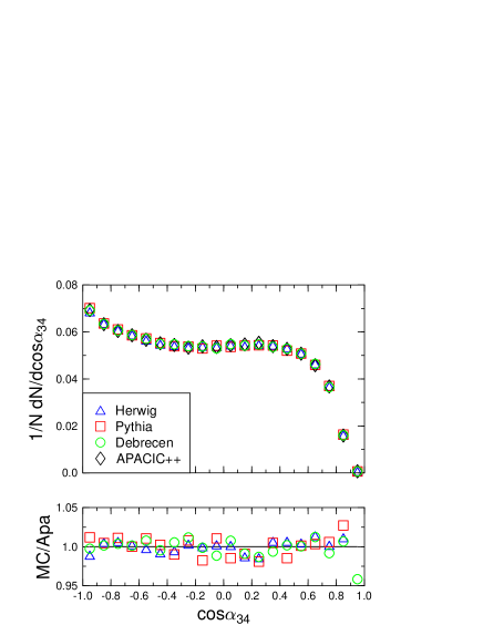
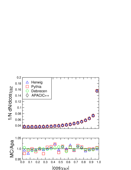
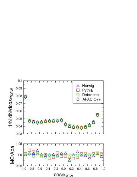
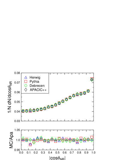
Figure 33: Comparison of LO–results on the level of matrix elements for the four jet angles with jets clustered at $y_{cut}^{D}=0.008$. The upper plots depict the normalized number of events per bin, the lower ones the ratios of Herwig, Pythia, Debrecen and Apacic++.

There is quite a large variety of programs featuring the production of four jets via QCD at the tree–level. Here, the performance of four of them, namely Herwig, Pythia, Debrecen and the package Apacic++/Amegic++ (denoted as Apacic++ in the following), is compared.

Note that according to the corresponding manuals, the four jet expressions within Pythia and Herwig are for massless partons (apart some mass effects which are built in for Pythia) and they contain only the structures to be found for the exchange of virtual photons [26]. However, the claim is, that the additional terms related to intermediate $Z$–bosons have only a minor effect [9]. At least for the observables studied here this claim has been verified.

The focus is on the observables defined in Sec. 5.2, specifically the four jet angles $\alpha_{34}$, $\chi_{BZ}$, $\phi_{KSW}$ and $\theta_{NR}$, and $y_{34}^{D}$, the $y_{c}$–value according to the Durham-scheme, where four–jet events turn to three resolvable jets. All results shown and discussed here are on the primary parton level, i.e., results obtained by the appropriate matrix elements squared, and at a centre-of-mass energy of $91.2$ GeV, with the argument of $\alpha_{\mbox{\tiny S}}$ kept fixed.

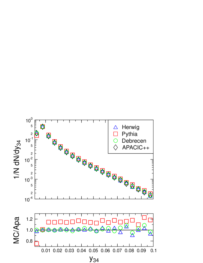
Figure 34: Comparison of LO–results for the $y_{34}^{D}$–distributions at the level of matrix elements. The upper plot exhibits the normalized number of events per bin, the lower one again the ratios of the other generators and Apacic++.

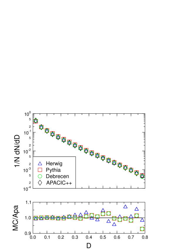
Figure 35: Comparison of LO–results for the $D$–parameter distributions at the level of matrix elements. The upper plot exhibits the normalized number of events per bin, the lower one again the ratios of the other generators and Apacic++.

The Monte–Carlo points were produced adopting the following strategy :

1. For Pythia a sample of four–jet events was generated with $y_{34}^{J}\geq y_{cut}^{J}=0.008$. This is due to the fact that in Pythia only the Jade scheme is available. Over a large region of phase space, as a rule of thumb, $y_{cut}^{J}\sim 4y_{cut}^{D}$ for the same kinematical configurations.

2. Out of this first sample, only events with $y_{34}^{D}\geq y_{cut}^{D}=0.004$ have been selected. For the other three generators, Herwig, Debrecen and Apacic++ the events were directly generated in the Durham-scheme with $y_{cut}^{D}=0.004$.

3. For the four jet angles, jets were defined according to $y_{cut}^{D}=0.008$, thus reducing the sample of step 2 by roughly $50\%$. For the $y_{34}$–distribution no additional cuts have been applied.
   

The resulting distributions of $\cos\alpha_{34}$, $|\cos\chi_{BZ}|$, $\cos\phi_{KSW}$ and $|\cos\theta_{NR}|$ can be found in Figure 33. Here, the upper plots exhibit the total number of events per corresponding bin normalized to the total number of events with $y_{cut}^{D}=0.008$, and in the lower plots the relative deviations from the Apacic++ results are displayed. With the exception of the last bin in $\cos\alpha_{34}$, the relative (statistical) errors on each distribution are of the size of the symbols. Clearly, the results show a satisfying coincidence with no sizeable relative deviations.

This situation changes when considering the $y_{34}^{D}$–distribution, see Figure 34. Again, the upper plot shows the normalized number of events per bin, and the lower plots depicts the relative deviations from the Apacic++ results. Here, the spread of the statistical errors covers a region from barely visible in the left bins up to three times the size of the symbols in the right bins. However, the deviations of the generators from each other are larger than their individual relative errors and reach up to $15\%$. Seemingly, Herwig, Debrecen and Apacic++ coincide. The results obtained by Pythia are somewhat – ${\cal O}(15\%)$ – higher, with the first bin as the only significant exception. Here, Pythia is well below ($\sim 25\%$) the other generators. However, it should be noted here, that this is probably due to the way the Pythia sample was produced. Since for the production of the Pythia sample in the first step the intrinsic Jade scheme was employed, deviations can be expected especially in the regions where the phase space is cut, i.e., for low $y_{34}$. Normalising in the region $y_{34}>0.01$, for example, would remove the discrepancy. Turning to the $D$–parameter, the different generators agree very well with each other. The relative errors reach roughly the size of the symbols for $D\approx 0.2$ and are of the order of $10\%$ in the last bin. Note that for the $D$–parameter as well as for the four jet angles, any difference seen in the $y_{34}$–distribution is washed out.

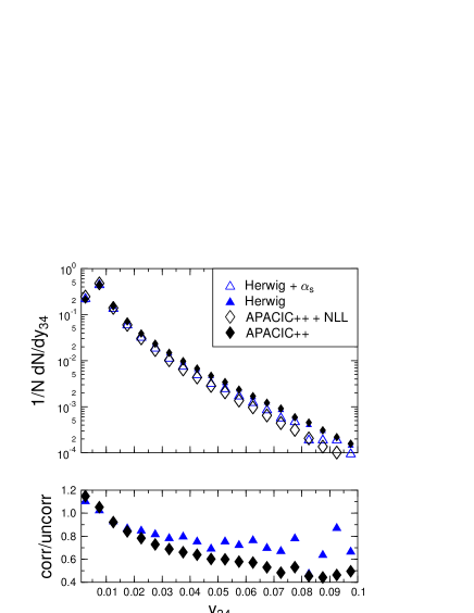
Figure 36: The shift in the $y_{34}^{D}$–distributions induced via the running of $\alpha_{\mbox{\tiny S}}$ in Herwig and the additional Sudakov weights in Apacic++. The upper plot shows the normalized number of events per bin, the lower one shows the ratios of the corrected versus the uncorrected version of each generator.

Herwig and Apacic++ provide additional options to supplement the pure matrix elements with running $\alpha_{\mbox{\tiny S}}$ instead of the fixed one with a scale depending on the specific kinematical situation (Herwig and Apacic++) or with some appropriate Sudakov weights (Apacic++), which depend on the flavours and the kinematics of the individual event. These two options are meant to model some aspects of higher order corrections to the pure LO matrix elements and result basically in a shift of events from regions with large $y_{34}$ to region with small $y_{34}$, see Figure 36. Here, the upper plot shows the number of events per bin in the $y_{34}$–distribution normalized to the total number of events and in the lower plot the ratio of the numbers per bin in the uncorrected and the corrected versions of the generators is depicted. The full and empty triangles correspond to Herwig without and with the running $\alpha_{\mbox{\tiny S}}$ option, the diamonds refer to Apacic++ without and with the Sudakov weights (“NLL”), respectively. Obviously, these options “soften” the $y_{34}$–distribution of the samples. On the other hand, their effect on the angular distributions is only minor in most of the phase space, see Figure 37. In the four plots the ratios of the corrected (corr) versus the uncorrected (uncorr) options for the four jet angles are displayed. It can be read off, that over the dominant region of phase space available, the inclusion of these corrections does not alter the angular distributions significantly. Rather, their effect is of the order of roughly $5\%$ with the only exception of the last bins for small $\alpha_{34}$, where the additional weights induce a drastical decrease of up to $15\%$. Note, however, that this region is strongly disfavoured, see the corresponding plot in Figure 33, thus, there are comparably large errors on the results.

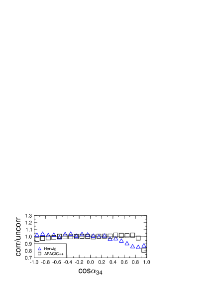
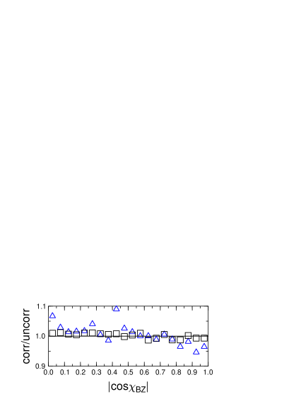
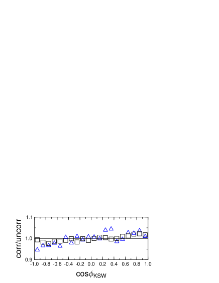
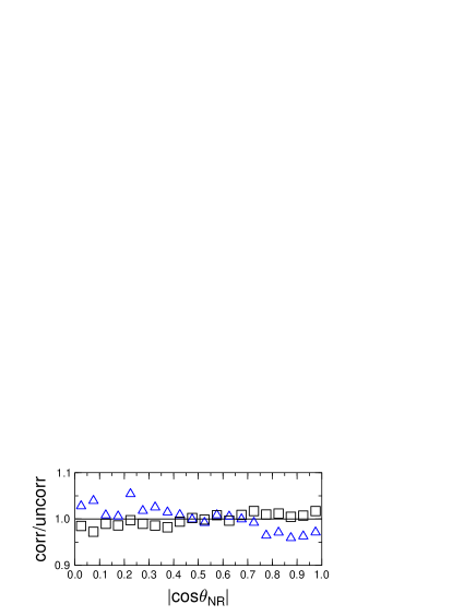
Figure 37: The ratio of the corrected and the uncorrected versions of Herwig and Apacic++ for the four jet angles.

5.3.2 Next-to-leading order corrections

For four-jet observables large differences were observed between LO order perturbative predictions and corrected experimental data. For instance, the LO perturbative result for the mean value of the D parameter is $\langle D\rangle^{LO}=0.0216$, while the experimental value is $0.0618\pm 0.0024$ [75], and even after including the large hadronization corrections, a significant discrepancy remains. Such a discrepancy and the large renormalization scale dependence of the LO preturbative result [58] shows clearly that if QCD is to work for four-jet observables, then there have to be large higher-order or non-perturbative corrections. On the other hand, the normalized angular distributions at LO are independent of the strong coupling, and therefore were expected to be insensitive to the renormalization scale, indicating small higher order corrections. For the clarification of the situation the NLO calculations were indispensable. During the second phase of Lep, four parton level NLO programs using different regularization methods were published, Menlo parc [54], Debrecen [58], Eerad2 [61] and Mercutio [62]. The one-loop matrix elements implemented in these codes were also different: Eerad2 uses the one-loop matrix elements of Ref. [76], while the other three programs implemented the one-loop matrix elements published in Ref. [77]. The results of the four programs were compared for distributions of many four-jet observables and very good agreement was found as exemplified here in Table 4, where the NLO four-jet fractions at three different $y_{\mathrm{cut}}$ values for the Durham clustering algorithm are compared. In the following, we shall present results obtained using the Debrecen code. This program is the only one of the four that gives the results in a colour decomposed form [78], which is useful for colour charge measurements.

Algorithm	$y_{cut}$	Menlo parc	Debrecen
	0.005	$(1.04\pm 0.02)\cdot 10^{-1}$	$(1.05\pm 0.01)\cdot 10^{-1}$
Durham	0.01	$(4.70\pm 0.06)\cdot 10^{-2}$	$(4.66\pm 0.02)\cdot 10^{-2}$
	0.03	$(6.82\pm 0.08)\cdot 10^{-3}$	$(6.87\pm 0.04)\cdot 10^{-3}$
	$y_{cut}$	Eerad2	Mercutio
	0.005	$(1.05\pm 0.01)\cdot 10^{-1}$	$(1.06\pm 0.01)\cdot 10^{-1}$
	0.01	$(4.65\pm 0.02)\cdot 10^{-2}$	$(4.72\pm 0.01)\cdot 10^{-2}$
	0.03	$(6.86\pm 0.03)\cdot 10^{-3}$	$(6.96\pm 0.03)\cdot 10^{-3}$

Table 4: The four-jet fraction as calculated by Menlo parc, Debrecen, Eerad2 and Mercutio, for the Durham jet algorithm.

The general form of the NLO differential cross section for a four-jet observable $O_{4}$ (for instance, D parameter, $O_{4}=D$, or Bengtsson-Zerwas angle, $O_{4}=\chi_{BZ}$) is given by the following equation:

$$\frac{1}{\sigma_{0}}\frac{d\sigma}{{\rm d}O_{4}}(O_{4})=\eta(\mu)^{2}\,B_{O_{4}}(O_{4})+\eta(\mu)^{3}\left[C_{O_{4}}(O_{4})+B_{O_{4}}(O_{4})\,\beta_{0}\,\ln(x_{\mu}^{2})\right]\>,$$ (46)

where $\sigma_{0}$ denotes the Born cross section for the process $e^{+}e^{-}\to\bar{q}q$, $\eta(\mu)=\alpha_{\mbox{\tiny S}}(\mu)\,C_{F}/(2\pi)$, $x_{\mu}$ is the ratio of the renormalization scale to the total centre-of-mass energy, and $B_{O_{4}}(O_{4})$, $C_{O_{4}}(O_{4})$ are the perturbatively calculable coefficient functions in the Born approximation and the radiative correction, respectively, which are independent of the renormalization scale.

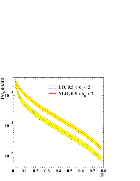
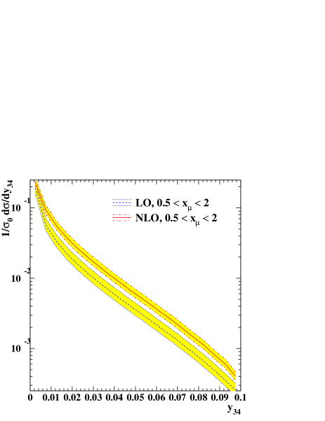
Figure 38: Comparison of the LO and NLO predictions for the D parameter (left) and the $y_{34}$ distribution (right). The shaded regions indicate the renormalization scale dependencies.

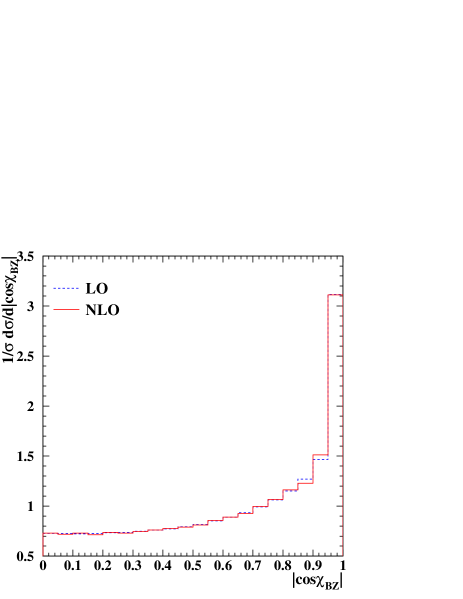
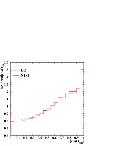
Figure 39: Comparison of the LO and NLO predictions for the Bengtsson-Zerwas (left) and the Nachtmann-Reiter distribution (right) for $x_{\mu}=1$.

We have performed a high statistics calculation of the $B$ and $C$ functions for the two event shape variables and for the four angular correlations defined in Sec. 5.2. Figure 38 shows the LO and NLO perturbative cross sections for the two event shapes. We observe that the inclusion of the radiative corrections increases the overall event rate substantially (by 70–130%). For instance, the mean value of the D parameter at NLO is $\langle D\rangle^{NLO}=0.0383(2)$, which is 77% larger than the LO value, but still far from the measured result. The NLO predictions exhibit significant renormalization scale dependence indicating the importance of even higher orders, which are not likely to be known in the foreseeable future. Thus, for event shapes the perturbative description remains unsatisfactory unless one attempts to use an optimized scale choice [61]. The only possible exception is the four-jet rate for the Durham algorithm, where the relative size of the NLO correction is around 60%, and the resummation of large logarithms exists [4]. Indeed, after matching the next-to-leading logarithmic and NLO results one finds a small renormalization scale dependence and a remarkably good description of the corrected experimental data [79].

The perturbative result is much more convincing in the case of the angular correlations, although the NLO calculations have brought some surprises, too. In Figure 39 we plot the LO and NLO perturbative predictions for the distributions of the Bengtsson-Zerwas and modified Nachtmann-Reiter angles. We see that the shapes of the distributions change very little when going from LO to NLO. However, when these predictions are used for measuring the QCD color factors, then, at NLO, one uses a quadratic form of the color charge ratios instead of the linear form used in a LO analysis [78]. The different functional form of the fitted function leads to different fitted parameters, even if the shape of the distribution is only slightly changed. In particular, the coefficient of the $T_{R}/C_{F}$ colour factor ratio receives a very large negative contribution leading to a significant shift in the measured value of this ratio if the NLO prediction is used instead of the LO one [60].

5.3.3 Mass corrections

For the investigation of mass effects Fourjphact and the package Apacic++/Amegic++ were used with the mass parameters of Table 5. Note that Apacic++ adds the value of a cutoff to the mass parameters, see Sec. 2.4.5.

	u	d	s	c	b
Fourjphact	0.35 GeV	0.35 GeV	0.5 GeV	1.5 GeV	4.8 GeV
Apacic++	0.01 GeV	0.01 GeV	0.2 GeV	1.7 GeV	4.7 GeV

Table 5: Quark mass values used for the generators Fourjphact and Apacic++.

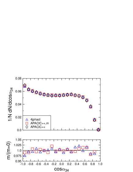
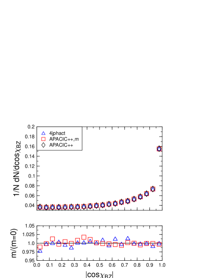
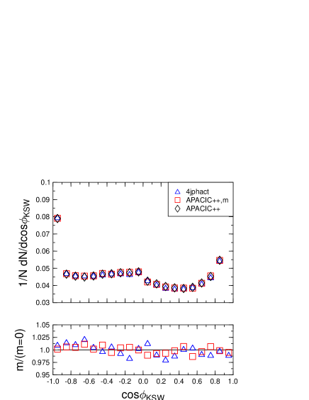
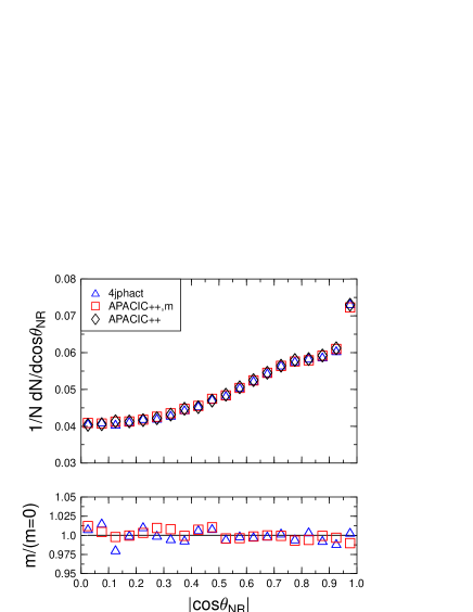
Figure 40: Comparison of massive and massless results for the four jet angles on the level of LO–matrix elements.

In general, the inclusion of masses has only a minor effect on the angular distributions. This result can be read off Figure 40. In the upper plots the massive distributions of Fourjphact  and Apacic++ are confronted with the massless result of Apacic++, and in the corresponding lower plots the ratios massive/massless are depicted. In most of the bins the effect of masses is of the order of $2\%$.

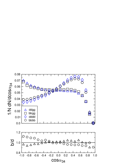
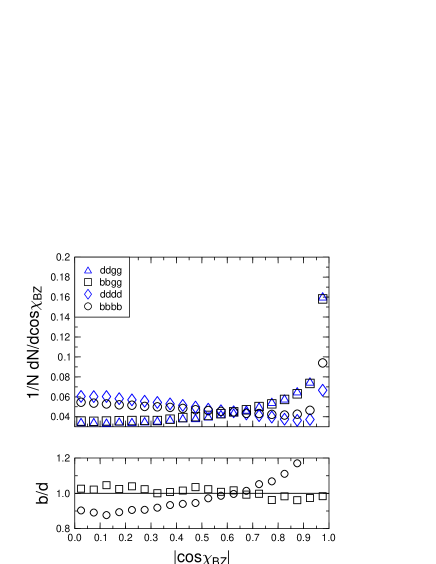
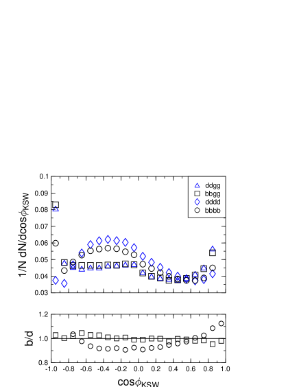
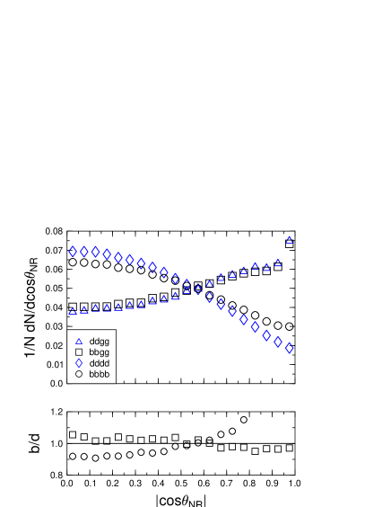
Figure 41: The four jet angles for some selected channels with and without masses.

This result is not too surprising, however, since only the $b$–quark mass induces any sizeable effect. In Figure 41, the results of different channels as given by Apacic++ are compared, namely $b\bar{b}b\bar{b}$, $b\bar{b}gg$, $d\bar{d}d\bar{d}$, and $d\bar{d}gg$. Again, in the upper plots the appropriately normalized number of events per bin is displayed for each channel, and the lower plots depict the corresponding ratios $(b\bar{b}b\bar{b})/(d\bar{d}d\bar{d})$ and $(b\bar{b}gg)/(d\bar{d}gg)$. Closer inspection of this figure reveals that the by far dominant four jet $b$ channel, namely $b\bar{b}gg$, is affected on the level well below $10\%$ in most of the phase space by mass effects. On the other hand, large effects, best seen in the comparison of $b\bar{b}b\bar{b}$ versus $d\bar{d}d\bar{d}$, are suppressed by the small relative rates of the corresponding channels.

In the $y_{34}$–distribution, mass effects are completely negligible, see Figure 42. In the upper plot, the $y_{34}$ distribution as given by Apacic++ with and without the inclusion of masses are depicted. The lower plot shows the ratios of the massive and the massless distributions. As expected, the inclusion of masses results in a slight shift from relatively soft (small $y_{34}$) to comparably hard (large $y_{34}$) events, since masses shield the collinear regions of particle emission. However, this effect is only of minor size, and in most bins the ratios massive/massless are quite close to 1. Large deviations can be seen in bins with limited statistics only.

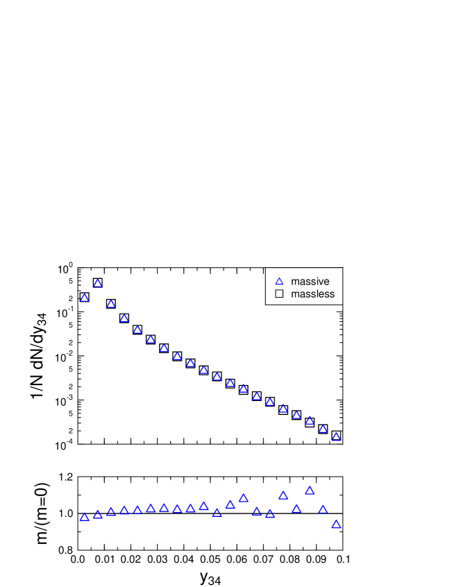
Figure 42: The $y_{34}^{D}$ distribution with and without the inclusion of masses.

5.3.4 Comparison of shower models

In this section we want to compare the predictions of various parton shower models. When working with the new MC options which allow for generating parton showers starting from a four-parton configuration, care has to be taken for particular aspects of these models. In order to avoid singularities in the four-parton generation according to the LO matrix elements, some intrinsic cut-off has to be applied for these programs, for example a Durham resolution criterion in case of Herwig. Therefore the resolution criterion with which jets are selected at the analysis level has to be larger than this intrinsic one. In case of Herwig, the intrinsic cut-off chosen is $y^{intr}_{cut}=0.004$, whereas jets are selected with $y_{cut}=0.008$. The analysis level can be the final state after the parton shower or after the hadronization step.

Attention has also to be paid to the edges of certain phase space regions, such as the end points in the angular distributions. These regions could be sensitive to the details in the implementations of the models, such as the handling of the masses and virtualities of the partons from which the parton showers start.

The hadronization parameters for the various models are taken from the tuned parameter sets as used by Aleph. No study with respect to variations in these parameters has been performed.

Figure 43: Comparison of Aleph data (preliminary, statistical errors only) to various MC model predictions for the four-jet angular distributions. Shown are also the ratios of the model predictions at hadron level. PY-4j=Pythia 6.1, 4-parton generation plus parton shower; HW-4j=Herwig 6.1, 4-parton generation plus parton shower; Fourjphact=4-parton generation including mass effects, parton shower via Pythia 6.1; PY-PS=Pythia 6.1, standard parton shower starting from a $q\bar{q}$ pair.

A study of the changes of the shapes for the angular distributions when going from parton to hadron level is outlined below in Sec. 5.4 for the case of Herwig. Here we concentrate on the comparison of the model predictions at hadron level, i.e., after parton showering and hadronization. Also shown is a comparison to data by Aleph. These data are preliminary, with statistical errors only, since the main purpose is to give a qualitative benchmark for the MC predictions. The data have been corrected for detector acceptance and resolution effects by means of bin-to-bin correction factors, as described in Sec. 5.2. The Monte Carlo program employed for this purpose is based on a standard parton shower approach, starting from a $q\bar{q}$ pair.

In case of the angular distributions, the normalization is with respect to the total number of four-jet events found, in order to concentrate on the shape. The event shape distributions are normalized to the total number of hadronic events generated.

From Figure 43 the following observations are made : The new option in Pythia 6.1, which interfaces a four-parton event to a parton shower, gives generally a very good description of the angular distributions, whereas the standard parton shower option shows deviations. The two other four-jet MC programs differ from the Pythia four-jet option by about 5-10%, with larger discrepancies seen only at the high end of the $\cos\alpha_{34}$ distribution, which is sensitive to mass effects and details of the implementation of the interface, since there two soft jets at close angles are probed. Quark mass effects, which are implemented in Fourjphact, do not have a sizeable impact on the shape of the distributions for the measured sample, which is a normal flavour mixture. However, when studying event samples enriched in heavy quarks, the mass effects should definitely be taken care of.

Figure 44: Comparison of Aleph data (preliminary, statistical errors only) to various MC model predictions for the event shape distributions $y_{34}$ and D parameter. Shown are also the ratios of the model predictions at hadron level. PY-4j=Pythia 6.1, 4-parton generation plus parton shower; HW-4j=Herwig 6.1, 4-parton generation plus parton shower; Fourjphact=4-parton generation including mass effects, parton shower via Pythia 6.1; PY-PS=Pythia 6.1, HW-PS=Herwig 6.1, standard parton shower starting from a $q\bar{q}$ pair.

In Figure 44 similar comparisons are shown for the event shape distributions $y_{34}$ and D parameter. Here a rather different picture arises. The four-jet MCs definitely fail to describe these distributions, whereas the standard parton shower approach gives good predictions apart from the very tails. This can be understood from the fact that the low end of the event shape distributions is rather sensitive to contributions from two- and three-jet events, which vanish at leading order in perturbative QCD, but can become sizeable after the parton shower simulation and after hadronization. These contributions are not implemented in the four-jet MC programs. Furthermore, the predictions for the low regions of the event shapes depend strongly on the intrinsic four-jet resolution parameter.

Therefore from these observations we conclude that the new four-jet MC options are well suited for the description of the shape of angular distributions in four-jet events, with remaining uncertainties of the order of 5%, if critical phase space regions are avoided. However, they cannot be used for observables which are sensitive to contributions from two- and three-jet events, which is the case for event shape distributions. Also the relative jet rates cannot be predicted correctly by these programs.

5.4 Hadronization corrections

A preliminary study of hadronization effects on the four-jet angular distributions was made using the Herwig four-jet matrix element + parton shower option, described in Sec. 2.2.4.

Figure 45: Parton- and hadron-level 4-jet angular distributions obtained with Herwig version 6.1 for light primary quarks, compared with matrix element.

Figure 46: Parton- and hadron-level 4-jet angular distributions obtained with Herwig version 6.1 for primary $b$ quarks, compared with matrix element.

Figures 45 and 46 show the distributions obtained at $s=M_{\mathrm{Z}}^{2}$ for light primary quarks (IPROC = 601) and primary $b$-quarks (IPROC = 605), respectively. The Durham jet metric was used with matrix-element cutoff Y4JT = $0.004$ and $y_{cut}=0.008$ for the actual resolution of jets. The dotted histograms show the matrix element distributions, with the argument of $\alpha_{\mbox{\tiny S}}$ running as explained in Sec. 2.2.4, while the dashed and solid ones are the reconstructed jet distributions at the parton level (after showering) and hadron level (after decays), respectively. In each case the distributions are normalized to the number of 4-jet events found (with $y_{cut}=0.008$) at the relevant level.

One sees that hadronization effects on the shapes of the 4-jet angular distributions are generally not large. The hadron/parton level ratios are, within the limited statistics of the present study, broadly similar to those obtained using the Herwig 2+3 jet ME+PS option (IPROC = 101,105). There are, however, indications that hadronization effects may be overestimated by the 2+3 jet ME+PS option at the 5-10% level in certain places, e.g. the central regions of $\theta_{NR}$ and $\chi_{BZ}$. Thus the use of correction factors obtained from the 2+3 jet ME+PS option needs to be treated with caution if precision better than 10% is required.

Close study of Figures 45 and 46 reveals the rather surprising fact that the hadron-level results are often closer than the parton-level ones to the (massless) matrix-element distributions. This is particularly true for primary $b$-quarks, suggesting that in Herwig the kinematic effects of the $b$-quark mass during parton showering are largely cancelled by the effects of hadronization and B-hadron decays.

Thus first results from the Herwig 4-jet ME+PS option suggest that hadronization effects are similar to those obtained using the old 2+3 jet option at the 10% level, and that effects of parton showering and hadronization tend to cancel in the 4-jet angular distributions. This should be investigated further as a function of c.m. energy and jet resolution. Further studies of 4-jet hadronization using the Pythia generator as well as the new combined 2,3 and 4 jet ME+PS Herwig option (see Sec. 2.2.5) are also needed.

5.5 Conclusions

A study of the description of 4-jet final states by various Monte Carlo models has been presented. Particular emphasis has been put on the comparison of new Monte Carlo generators, which produce 4-parton final states according to the leading order QCD matrix elements, and then add a parton shower and hadronization. In general good agreement between the different generators has been found. These new models give a better description of 4-jet angular distributions than the standard parton shower models, where the parton shower starts from a quark-antiquark initial state, only. However, jet rates as well as event shape distributions sensitive to 4-jet production, such as $y_{34}$, cannot be described by these models, since here also the contributions from 2- and 3-jet events are important. These observations should be taken into account when using the 4-jet MCs for background studies.

Quark mass effects are small for the distributions under consideration, for samples with normal flavour mixture. NLO contributions have minor impact on the shape of 4-jet angular distributions, but they change considerably the 4-jet rate and event shape distributions such as the D parameter. Possible large non-perturbative power corrections to observables such as the mean value of the D parameter have not been studied here.

A preliminary study of hadronization effects on 4-jet angular distributions, using the 4-jet ME+PS option of the Herwig generator only, showed with limited statistics that such effects are broadly similar to those seen with the 2+3 jet ME+PS option, although differences at the 5-10% level are apparent in certain configurations.

6 B QUARK FRAGMENTATION FUNCTION

Heavy quark fragmentation functions are a powerful tool in testing the predictivity of perturbative QCD (pQCD), since effects of non-perturbative origin are much more limited in size than in the light-flavour case. At the origin of this behaviour lies the fact that the mass $m$ of the heavy quark is much larger than the QCD scale $\Lambda$.

Indeed, on one side the large mass acts as an infrared cutoff for the mass singularities which would appear in the perturbative calculation, ensuring a finite result. The energy distribution of the $b$ quark prior to hadronization can therefore be calculated perturbatively. On the other side, hadronization effects have to be phenomenologically modelled, but happen to be small: a heavy quark only loses a momentum fraction of order $\Lambda/m$ when binding with a light one to form a heavy-light meson [90].

6.1 Experimental results

Results for the normalized energy distribution of $B$ hadrons, i.e.

$$D(Q,x_{E})\equiv{1\over\sigma}{d\sigma\over{dx_{E}}}\;,$$ (47)

in $e^{+}e^{-}$ collisions are given by the Lep collaborations and by the Sld experiment at SLC, at $Q=M_{\mathrm{Z}}$. The scaling variable $x_{E}$ is given by the ratio of the observed $B$ particle energy to the beam energy $E_{beam}$.

$\langle x_{E}\rangle$	$B$	Expt
0.7394$\pm$0.0054(stat)$\pm$0.0057(syst)	L	Aleph 2000  [91]
0.7198$\pm$0.0045(stat)$\pm$0.0053(syst)	wd	Aleph 2000  [91]
0.714$\pm$0.005(stat)$\pm$0.007(syst)$\pm$0.002(mod)	wd	Sld 1999  [92]
0.702$\pm$0.008	wd	Lep HFWG avg. 1996  [93]
0.695$\pm$0.006(stat)$\pm$0.003(syst)$\pm$0.007(mod)	wd	Opal 1995  [94]
0.716$\pm$0.0006(stat)$\pm$0.007(syst)	L	Delphi 1995  [95]

Table 6: Mean scaled energy of $B$ hadrons from various $e^{+}e^{-}$ experiments at $Q=M_{\mathrm{Z}}$.

A typical observable measured by experiments is the mean scaled energy fraction $\langle x_{E}\rangle$. Table 6 shows some of the most recent determinations of this quantity. In this table the second column identifies the kind of $B$ particle observed in the final state, be it the “leading” (also called “primary”) (L) or the “weakly decaying” one (wd). Of course, the average energy of the latter is lower than that of the former, since it has undergone further decaying processes. It should also be noted that the precise details of what the observed final state actually is will at least slightly vary from experiment to experiment. The numbers quoted in the table under the same label “wd” are therefore not exactly comparable, though probably homogeneous enough within the experimental uncertainties so that one can average them. Needless to say, it would be useful if all analyses at some point finally agreed on a single definition for this final state.

The most recent analyses also report fairly accurate data for the full fragmentation function eq. (47), with $x_{E}$ ranging from near zero to one. As expected, these distributions peak very close to one, around $x_{E}\simeq$ 0.8-0.9.

6.2 Theoretical predictions

The challenge for the theoretical calculations is of course to reproduce not only the mean scaled energy but also, as far as possible, the full fragmentation distribution. A certain degree of phenomenological modelling will be necessary, as perturbative calculations cannot of course describe the hadronization of the $b$ quark into $B$ mesons and/or baryons. The full fragmentation function is therefore usually described in terms of a convolution between a calculable perturbative component and a phenomenological one:

$$D(Q,x;m,\Lambda;\epsilon_{1},\ldots,\epsilon_{n})=D^{pert}(Q,x;m,\Lambda)\otimes D^{np}(x;\epsilon_{1},\ldots,\epsilon_{n})\;.$$ (48)

In this equation the perturbative component depends on the centre-of-mass energy $Q$, the QCD coupling and the heavy quark pole mass $m$, while the non-perturbative one is assumed to depend only on some given set of phenomenological parameters $(\epsilon_{1},\ldots,\epsilon_{n})$, to be determined by fitting the experimental data.

The perturbative component can be either calculated by analytical means or extracted from Monte Carlo simulations of the emission of radiation by the fragmenting heavy quark. In the latter case the theoretical accuracy will of course be lower.

As far as fixed order analytical calculations are concerned, today’s state of the art is the work of ref. [96]. It is accurate up to order $\alpha_{\mbox{\tiny S}}^{2}$ and also fully includes finite mass terms of the form $(m/Q)^{p}$ with $p\geq 1$.

Fixed order results do however display two classes of large logarithmic terms: collinear logs, of the form $\log(Q^{2}/m^{2})$, and Sudakov logs, $\log(1-x)$. These terms become large when the centre-of-mass energy is much larger than the heavy quark mass, a fact certainly true at Lep and Sld, and at the $x\simeq 1$ endpoint respectively. All-order resummations for such terms, very important for producing a reliable result, have and are being considered [97], and are now available at next-to-leading log (NLL) accuracy for both classes of logarithms. Ref. [96] also provides a merging between the fixed order calculation and the collinear-resummed one.

Once pQCD has produced a reliable prediction for the $b$ quark fragmentation, one has to “dress” it with some phenomenological modelling in order to describe the observed $B$ hadrons distribution, as discussed before. It is important to realize that, since only the convolution of the two factors in Eq. 48 has physical meaning, the parameters fitted in the non-perturbative part will strictly depend on the kind of description adopted for the perturbative term. Different descriptions and/or different parameters in $D^{pert}(Q,x;m,\Lambda)$ will lead to different values for the fitted $(\epsilon_{1},\ldots,\epsilon_{n})$ set. Once fitted, such a set will therefore not be usable in conjunction with perturbative descriptions other than the one it has been fitted with.

$\langle x_{E}\rangle_{pert}$	$\Lambda_{5}=100$ MeV	$\Lambda_{5}=200$ MeV	$\Lambda_{5}=300$ MeV
$m_{b}=4$ GeV	0.790	0.753	0.723
$m_{b}=4.5$ GeV	0.802	0.767	0.740
$m_{b}=5$ GeV	0.813	0.780	0.755

Table 7: Perturbative predictions for $\langle x_{E}\rangle_{pert}$ at $Q=91$ GeV, for different values of $m_{b}$ and $\Lambda_{5}$.

As an example, Table 7 shows the average scaled energy value of the $b$ quark after fragmentation, $\langle x_{E}\rangle_{pert}$, as predicted by the perturbative term only, for different values of $\Lambda$ and $m$. The calculation used in this example resums to NLL accuracy both collinear and Sudakov logs, but neglects the non-logarithmic finite mass terms. One can clearly see that, on one hand, the purely perturbative predictions are too large to directly describe the experimental results, unless probably unrealistic value for $\Lambda_{5}$ and $m_{b}$ are used. On the other hand, each different $(m_{b},\Lambda_{5})$ choice will of course imply a different fitted value for the non-perturbative parameters if the same measured $\langle x_{E}\rangle$ is to be correctly described.

While the calculation of the perturbative component does of course follow the rules dictated by pQCD, much more freedom is instead available when choosing the form of the non-perturbative contribution $D^{np}(x)$. A lot of different parametrizations have been employed and can be found in the literature: some of them possibly more physically motivated, some chosen only because of practical advantages like an easy Mellin transform or enough parameters to ensure that the shape of the data can be properly described. A list, probably incomplete, of these functional forms can be found in [98], though it should be noted that some of them appear now to be disfavoured by comparisons with experimental data.

As an example of such a comparison, let us consider one of the best-sellers of these non-perturbative forms, namely the Peterson et al. fragmentation function. Such a function is meant to be one of the physically motivated ones, and has the attractive feature of depending on only one phenomenological parameter $\epsilon$, which can moreover be roughly related to more fundamental quantities via the relation $\epsilon\sim\Lambda^{2}/m^{2}$. This function reads

$$D^{np}(x;\epsilon)=N(\epsilon){1\over x}\left(1-{1\over x}-{\epsilon\over{1-x}}\right)^{-2}$$ (49)

where $N(\epsilon)$ is the normalization factor.

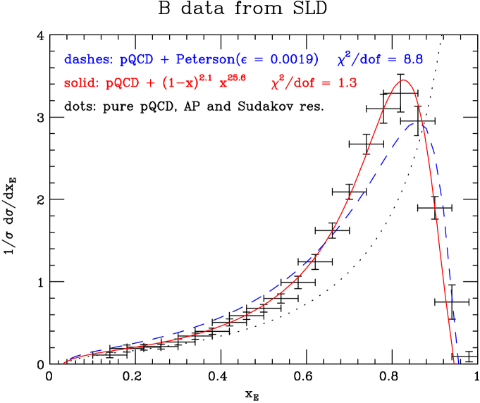
Figure 47: The data from Sld [92] and two theoretical fits. The pQCD prediction is in all cases collinear (or AP, for Altarelli-Parisi) and Sudakov resummed.

The plot in Figure 47 shows the result of attempting a point-by-point fit of the Peterson form, convoluted with the same perturbative calculation used in Table 7, to the latest data from Sld. It can be clearly appreciated how the Peterson model, coupled to this perturbative description, does not seem to offer a valid description of the data. The same conclusion was reached by the Sld Collaboration by coupling this model to the Jetset Monte Carlo description of the perturbative component.

It should however be noted that Eq. 49 was derived under the assumption of describing the hadronization of a heavy quark into a heavy-light meson by picking up a light quark from the vacuum. No attempt was made to include the description of the subsequent decays transforming the leading $B$ particle into the weakly decaying ones, which are the ones observed here. Such decays will modify the shape of the fragmentation function, and might at least partially explain the observed discrepancy.

Figure 47 also shows a fit performed with a different non-perturbative function, namely

$$D^{np}(x;\alpha,\beta)=N(\alpha,\beta)(1-x)^{\alpha}x^{\beta}\;.$$ (50)

This particular form has no immediate physical origin, but it is often used because it has a very simple Mellin transform and is flexible enough to describe the data well. One can indeed see from the plot that it allows for a very good fit of the experimental data.

6.3 Monte Carlo predictions

An important issue that remains to be addressed is the performance of the main Monte Carlo event generators in comparison with the latest data on $b$-quark fragmentation. Figure 48 shows the results of combining Jetset (version 7.4) parton showers with various models [98] for $b$-quark fragmentation into a weakly-decaying B-hadron, compared to the recent Sld data [92]. Jetset plus Lund fragmentation gives a good description of the data whereas, as was the case in the analytical calculations discussed above, the Peterson model does not.

The prediction from Herwig (version 5.7) is seen to be too soft in comparison to the Sld data. As already remarked in Sec. 2.2.3, a harder B-hadron spectrum can be obtained in Herwig 6.1 by varying the $b$-quark fragmentation parameters separately. However, detailed tuning of version 6.1 to these data has not yet been attempted.

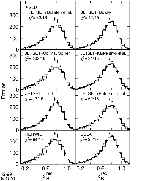
Figure 48: B-fragmentation data from Sld [92] compared with various models.

6.4 Concluding remarks

Accurate theoretical preditions exist for the perturbative part of the heavy quark fragmentation function. Collinear and Sudakov logarithms can be resummed to next-to-leading accuracy, and the finite mass terms are known up to order $\alpha_{\mbox{\tiny S}}^{2}$. All the various contributions can be merged into a single result.

On top of this perturbative result a non-perturbative contribution will always have to be included, and precise experimental data can help identifying the proper shape for such a function.

Predictions for heavy quark fragmentation from the latest versions of Monte Carlo generators have yet to be compared and tuned to the most recent data.

7 GLUON SPLITTING INTO BOTTOM QUARKS

7.1 Experimental data

The current experimental results on the quantity

$$g_{bb}=\frac{\Gamma(Z^{0}\to q\bar{q}g,g\to b\bar{b})}{\Gamma(Z^{0}\to\mbox{hadrons})}$$

are summarized in Table 8. The first three results are based on extracting a secondary $b\bar{b}$ signal from a 4-jet sample, whereas the latest Delphi value is obtained from a measurement of the 4$b$ rate $\Gamma(Z^{0}\to b\bar{b}b\bar{b})$, which should be less model-dependent and give better phase-space coverage.

Experiment	Ref.	$g_{bb}$ (%)
Delphi	[100]	$0.21\pm 0.11\pm 0.09$
Aleph	[101]	$0.277\pm 0.042\pm 0.057$
Sld	[102]	$0.307\pm 0.071\pm 0.066$
Delphi	[103]	$0.33\pm 0.10\pm 0.08$

Table 8: Experimental data on gluon splitting to $b\bar{b}$.

7.2 Analytical predictions

References [104, 105, 106] give leading-order [${\cal O}(\alpha_{\mbox{\tiny S}}^{2})$] predictions as well as the results of resummation of leading [$\alpha_{\mbox{\tiny S}}^{n}\log^{2n-1}(s/m_{b}^{2})$] and next-to-leading [$\alpha_{\mbox{\tiny S}}^{n}\log^{2n-2}(s/m_{b}^{2})$] logarithms (NLL) to all orders in $\alpha_{\mbox{\tiny S}}$, matched with leading order. The results, for $\alpha_{\mbox{\tiny S}}=0.118$, $s=M_{\mathrm{Z}}^{2}$ and $m_{b}=5.0$ GeV, are summarized in Table 9.

Calculation	$g_{bb}$ (%)
Leading order	0.110
LO + NLL [105]	0.207
LO + NLL [106]	0.175

Table 9: Calculations of gluon splitting to $b\bar{b}$.

We see that resummation of logarithms gives a substantial enhancement. Bearing in mind that $\log(M_{\mathrm{Z}}^{2}/m_{b}^{2})\simeq 6$ and $\alpha_{\mbox{\tiny S}}\log^{2}(M_{\mathrm{Z}}^{2}/m_{b}^{2})\simeq 4$, this is not surprising. Still missing are higher-order terms of the form $\alpha_{\mbox{\tiny S}}^{n}\log^{2n-m}(s/m_{b}^{2})$ with $n,m>2$, which could well become comparable with the leading term at high orders. The difference between the predictions of [105] and [106] is due to their different treatment of NNLL ($m=3$) terms.

In conclusion, the theoretical prediction for $g_{bb}$ must still be regarded as quite uncertain, and not in serious disagreement with the data.

Reference [106] also contains predictions of secondary heavy quark production as a function of an event shape variable (the heavy jet mass). There are no data available yet on this, so the authors compare with Monte Carlo results. Their predictions are similar to those of the main event generators discussed below.

Monte Carlo predictions of $g_{bb}$ are in principle even more unreliable than the theoretical results presented above, since they do not fully include next-to-leading logarithms or matching to fixed order. Nevertheless they do include some real effects absent from the analytical calculations, such as the effects of phase-space limitations. Different options for the treatment of subleading terms, such as the choice of argument for $\alpha_{\mbox{\tiny S}}$, can easily be explored by providing suitable switches in the programs. Also of course they provide a complete model of the final state, which allows the effects of experimental cuts to be simulated. Relevant developments in the main Monte Carlo programs are described in the following three subsections.

7.3 Monte Carlo developments: PYTHIA

7.3.1 Strong coupling argument and kinematics

The default behaviour in Pythia is to let $\alpha_{\mbox{\tiny S}}$ have $p_{T}^{2}$ as argument. Actually, since the exact kinematics has not yet been reconstructed when $\alpha_{\mbox{\tiny S}}$ is needed, the squared transverse momentum is represented by the approximate expression $z(1-z)m^{2}$, where $z$ is the longitudinal splitting variable and $m$ the mass of the branching parton. Since $\alpha_{\mbox{\tiny S}}$ blows up when its argument approaches $\Lambda_{QCD}$, this translates into a requirement on $p_{T}^{2}$ or on $z$ and $m$, restricting allowed emissions to $p_{T}>Q_{0}/2$, where $Q_{0}$ is the shower cutoff scale. Also when full kinematics is reconstructed, this is reflected in a suppression of branchings with small $p_{T}$. Therefore, if the angular distribution of the $g$ decay is plotted in its rest frame, the quarks do not come out with the $1+\cos^{2}\theta$ angular distribution one might expect, but rather something peaked at $90^{\mbox{\scriptsize o}}$ and dying out at $0^{\mbox{\scriptsize o}}$ and $180^{\mbox{\scriptsize o}}$.

For $g\to q\bar{q}$ branchings, the soft-gluon results that lead to the choice of $p_{T}^{2}$ as scale are no longer compelling, however. One could instead use some other scale that does not depend on $z$ but only on $m$. A reasonable, but not unique, choice is to use $m^{2}/4$, where the factor 4 ensures continuity with $p_{T}^{2}$ for $z=1/2$. This possibility has been added as new option MSTJ(44)=3. In order for this new option to be fully helpful, a few details in the treatment of the kinematics have also been changed for the $g\to q\bar{q}$ branchings. These changes are not completely unimportant, but small on the scale of the other effects discussed here.

Actually, the change of $\alpha_{\mbox{\tiny S}}$ argument in itself leads to a reduced $g\to q\bar{q}$ splitting rate, while the removal of the $p_{T}>Q_{0}/2$ requirement increases it. The net result is an essentially unchanged rate, actually decreased by about 10% for charm and maybe 20% for bottom, based on not overwhelming statistics. The kinematics of the events is changed, so experimental consequences would have to be better quantified. However, the changes are not as big as might have been expected – see the following.

7.3.2 Coherence

In the above subsection, it appears as if the $1+\cos^{2}\theta$ distribution would be recovered in the new option MSTJ(44)=3. However, this neglects the coherence condition, which is imposed as a requirement in the shower that successive opening angles in branchings become smaller. Such a condition actually disfavours branchings with $z$ close to 0 or 1, since the opening angle becomes large in this limit. It should be noted that the opening angle discussed here is not the true one, but the one based on approximate kinematics, including neglect of masses. One may question whether the coherence arguments are really watertight for these branchings, especially if one considers $g\to q\bar{q}$ close to threshold, where the actual kinematics is quite different from the one assumed in the massless limit used in the normal coherence derivation.

As a means to exploring consequences, two new coherence level options MSTJ(42)=3 and 4 have thus been introduced. In the first, the $p_{T}^{2}$ of a $g\to q\bar{q}$ branching is reduced by the correct mass-dependent term, $1-4m_{q}^{2}/m_{g}^{2}$, while the massless approximation is kept for the longitudinal momentum. This is fully within the uncertainty of the game, and no less reasonable than the default MSTJ(42)=2. In the second, no angular ordering at all is imposed on $g\to q\bar{q}$ branchings. This is certainly an extreme scenario, and should be used with caution. However, it is still interesting to see what it leads to.

It turns out that the decay angle distribution of the gluon is much more distorted by the coherence than by the $\alpha_{\mbox{\tiny S}}$ and kinematics considerations described earlier. Both modifications are required if one would like to have a $1+\cos^{2}\theta$ shape, however. Also other distributions, like gluon mass and energy, are affected by the choice of options.

The most dramatic effect appears in the total gluon branching rate, however. Already the introduction of the mass-dependent factor in the angular ordering requirement can boost the $g\to b\bar{b}$ rate by about a factor of two. The effects are even bigger without any angular ordering constraints at all. It is difficult to know what to make of these big effects. The options described here would not have been explored had it not been for the Lep data that seem to indicate a very high secondary charm and bottom production rate. Experimental information on the angular distribution of secondary $c\bar{c}$ pairs might help understand what is going on better, but probably that is not possible experimentally.

7.3.3 Summary

In order to study uncertainties in the $g\to b\bar{b}$ rate, some new Pythia options have been introduced, MSTJ(44)=3 and MSTJ(42)=3 and 4, none of them as default (yet). Taken together, they can raise the $g\to b\bar{b}$ rate by a significant factor, as summarized in Table 10. A study of the effects of these options on the 3-jet rate ratio $R_{4}^{b\ell}$ is described in Sec. 4.4.4.

MSTJ(44)	MSTJ(42)	$g_{uu+dd+ss}$ (%)	$g_{cc}$ (%)	$g_{bb}$ (%)
($\alpha_{\mbox{\tiny S}}$)	(coherence)
2	2	14.3	1.26	0.16
2	3	20.9	1.93	0.26
2	4	38.5	3.07	0.32
3	2	12.9	1.16	0.15
3	3	19.9	1.77	0.28
3	4	42.9	3.48	0.46

Table 10: Pythia options for gluon splitting to $q\bar{q}$. Rates at 91.2 GeV for the normal flavour mixture.

The MSTJ(42)=4 option is clearly extreme, and to be used with caution, whereas the others are within the (considerable) range of uncertainty.

The corrections and new options are available starting with Pythia 6.130, obtainable from
www.thep.lu.se/$\sim$torbjorn/Pythia.html.

7.4 Monte Carlo developments: HERWIG

7.4.1 Angular distribution in $g\to q\bar{q}$

In Herwig, the angular-ordering constraint, which is derived for soft gluon emission, is applied to all parton shower vertices, including $g\to q\bar{q}$. In versions before 6.1, this resulted in a severe suppression (an absence in fact) of configurations in which the gluon energy is very unevenly shared between the quarks. For light quarks this is irrelevant, because in this region one is dominated by gluon emissions, which are correctly treated. However for heavy quarks, this energy sharing (or equivalently the quarks’ angular distribution in their rest frame) is a directly measurable quantity, and was badly described.

Related to this was an inconsistency in the calculation of the Sudakov form factor for $g\to q\bar{q}$. This was calculated using the entire allowed kinematic range (with massless kinematics) for the energy fraction $x$, $0\leq x\leq 1$, while the $x$ distribution generated was actually confined to the angular-ordered region, $x,1\!-\!x\geq m/\sqrt{E^{2}\xi}$ (see Sec. 2.2.1).

In Herwig version 6.1, these defects are corrected as follows. We generate the $E^{2}\xi$ and $x$ values for the shower as before. We then apply an a posteriori adjustment to the kinematics of the $g\to q\bar{q}$ vertex during the kinematic reconstruction. At this stage, the masses of the $q$ and $\bar{q}$ showers are known. We can therefore guarantee to stay within the kinematically allowed region. In fact, the adjustment we perform is purely of the angular distribution of the $q$ and $\bar{q}$ showers in the $g$ rest frame, preserving all the masses and the gluon four-momentum. Therefore we do not disturb the kinematics of the rest of the shower at all.

Although this cures the inconsistency above, it actually introduces a new one: the upper limit for subsequent emission is calculated from the generated $E^{2}\xi$ and $x$ values, rather than from the finally-used kinematics. This correlation is of NNL importance, so we can formally neglect it. It would be manifested in an incorrect correlation between the masses and directions of the produced $q$ and $\bar{q}$ jets. This is, in principle, physically measurable, but it seems less important than getting the angular distribution itself right. In fact the solution we propose maps the old angular distribution smoothly onto the new, so the sign of the correlation will still be preserved, even if the magnitude is wrong.

Even with this modification, the Herwig  kinematic reconstruction can only cope with particles that are emitted into the forward hemisphere in the showering frame. Thus one cannot populate the whole of kinematically-allowed phase space. Nevertheless, we find that this is usually a rather weak condition, and that most of phase space is actually populated.

Using this procedure, we find that the predicted angular distribution for secondary $b$ quarks at Lep energies is well-behaved, i.e. it looks reasonably similar to the leading-order result ($1+\cos^{2}\theta^{*}$), and has relatively small hadronization corrections.

7.4.2 Predictions for $g_{bb}$

Reference [105] contains comparisons between analytical predictions for $g_{bb}$ and those of Herwig. One result of the analytical calculation is that, to NLL accuracy, one can use the massless formula for the splitting $g\to b\bar{b}$, provided one also sets a cutoff on the virtual gluon mass of $m_{g}>e^{5/6}m_{b}=2.3m_{b}$ instead of the kinematic cutoff $m_{g}>2m_{b}$. Somewhat fortuitously, this is similar to the Herwig method, which uses the massless formula with a cutoff $m_{g}>2(m_{b}+Q_{0})$ with $Q_{0}\simeq 0.5$ GeV. The comparisons in show that the resummed and Herwig predictions are quite similar at Lep1 and Lep2 energies.

Herwig results for $Z^{0}$ decay are summarized in Table 11, for the version used in the original comparisons (5.7) and the latest version, 6.1 [23]. The main difference between the two versions in this context is a change in the default $b$-quark mass from $m_{b}=5.2$ GeV to 4.95 GeV, which is justified by the approximate relation $m_{B}=m_{b}+m_{l}$ where $m_{l}$ is the light quark mass. We see that the Herwig results are somewhat higher than the resummed predictions in Table 9 and in better agreement with the data in Table 8.

Version	$g_{bb}$ (%)
5.7	0.23
6.1	0.25

Table 11: Herwig predictions for gluon splitting to $b\bar{b}$.

7.5 Monte Carlo developments: ARIADNE

The splitting of gluons into a $q\bar{q}$ pair does not fit into the dipole picture in an obvious way, since this splitting is related directly to a single gluon rather than to any dipole between two partons. Also, all gluons in emitted in the cascade are massless, and to be able to split into massive quarks, energy has to be required from somewhere. The way the process is included in Ariadne is described in ref. [107] The splitting probability of a gluon is simply divided in two equal parts, each of which is associated to each of the two connecting dipoles. The splitting process can then again be treated as a two-to-three process, where a spectator parton is used to conserve energy and momentum. It can be shown that this is equivalent to standard parton shower approaches in the limit of strongly ordered emssions. But the differences when extrapolating away from that limit can become large, and Ariadne typically gives twice as many secondary b$\bar{\mbox{b}}$ pairs as compared to eg. Jetset.

But this treatment of secondary heavy quarks may lead to rather strange situations (as noted in ref. [33]). Since transverse momentum of the $q\bar{q}$ splitting can become small even for heavy quarks, it is possible to split a gluon so that the mass $m_{q\bar{q}}^{2}$ is larger than the transverse momentum scale – $p_{\perp g}^{2}$ – at which the gluon was emitted – although the ordering of the emissions, $p_{\perp q\bar{q}}^{2}<p_{\perp g}^{2}$, is still respected. To avoid such situations there is an option in Ariadne which introduces an extra limit, $m_{q\bar{q}}^{2}<p_{\perp g}^{2}$, on gluon splitting.

As discussed already in Sec. 7.3, it is not quite clear if or how the ordering of emissions should be enforced in the case of gluon splitting into massive quarks and, for that reason, Ariadne also includes an option where these splittings are allowed to be non-ordered, ie. $p_{\perp q\bar{q}}$ is allowed to be larger than the transverse momentum of the preceeding emission. The corresponding rates of gluon splittings are given in table 12

MSTA(28)	$g_{u\bar{u}+d\bar{d}+s\bar{s}}$	$g_{c\bar{c}}$	$g_{b\bar{b}}$
0	25.9	2.18	0.34
1	17.7	1.09	0.13
–1	28.8	1.88	0.16

Table 12: Ariadne options for gluon splitting into $q\bar{q}$. Rates at 91.2 GeV for the normal flavour mixture.

8 OVERALL CONCLUSIONS AND RECOMMENDATIONS

Here we summarise the main results from each Section above and the recommendations that follow from them. The term ‘jet rates’ always refers to the Durham algorithm unless it is explicitly stated otherwise.

8.1 Monte-Carlo developments

The relevant features of the main event generators, Pythia, Herwig and Ariadne, were reviewed with emphasis on relevant new developments. In many cases, important modifications and new options were introduced as a result of discussions in the working group.

In Pythia, improved treatment of quark masses in the parton shower permits a better description of the overall 3-jet rate, but there remains a problem of underestimation of the 4-jet rate. Modification of the way in which matrix element corrections are applied has little effect on this.

In Herwig, parameters for the cluster hadronization of $b$-quarks have been separated from those for ligher quarks, so that improved tuning to $b$-quark fragmentation data will be possible.

In both Pythia and Herwig there are now options to interface parton showers to the massless 4-parton matrix elements. In addition, Fourjphact interfaces the massive 4-parton matrix elements to Pythia parton showers. These options provide an improved description of 4-jet final states, but are not suitable for describing features that receive important 2- and 3-jet contributions. A very recent development in Herwig is an option to combine 2,3 and (massless) 4-parton matrix elements together with parton showers in a way that aims to avoid the worst aspects of double counting. Comparison and tuning of this option to Lep1 data is in progress.

In Ariadne, options exist for switching on and off the dead-cone effect in QCD radiation from heavy quarks. A massive leading-order matrix element correction has also been introduced, as exists in Pythia and Herwig. Overall, Ariadne gives a better description of jet rates than either Pythia or Herwig. However, the description of mass effects in jet rates in Ariadne is not so satisfactory, and in fact turning off the treatment of quark masses altogether appears to provide a better description.

A major new development is the introduction of the new event generator Apacic++, which for the first time interfaces $n$-parton matrix elements and parton showers for $n=2,\ldots,5$. A number of options are available for choosing the relative jet rates, and for initialising and evolving the parton showers. As in Pythia and Ariadne, the Jetset string hadronisation model is used. A first attempt at tuning to Lep1 data gives encouraging results, with fits to most event shape and single-particle distributions of a quality similar to the established generators. Differential jet rates show some features which may be associated with merging the different parton multiplicities. The tuned shower cutoff is high, so that the parton showers have little phase space for evolution and final-state structure is mostly determined by matrix elements and hadronization.

8.2 Jet rates (inclusive)

Both Pythia and Herwig have problems with fitting the 3- and 4-jet rates simultaneously as functions of the jet resolution $y_{c}$. For a given tuning, one can describe e.g. the 3-jet rate well, but then the rates for higher jet multiplicities are overestimated by Herwig and underestimated by Pythia. None of the modifications tried was able to eliminate this problem. For analyses at Lep2 energies using Pythia or Herwig, we recommend tuning to the relevant jet rate at Lep1 in order to minimize the associated systematic error, which then results only from the change in that jet rate from Lep1 to Lep2. If this is done, then a systematic error of 2% in the 4-jet rate at Lep2 could be achieved. On the other hand, if only a general tuning at Lep1 is performed, the systematic error could be as large as 5%.

Ariadne gives the best overall description of jet rates and should therefore be considered as the generator of choice for estimating multi-jet backgrounds, e.g. in hadronic WW decay studies. Using Ariadne could lead to a further reduction of systematic errors.

8.3 Jet rates (mass effects)

Full NLO massive matrix element calculations of the 3-jet rate are now available. They were used to study the effect of the $b$-quark mass on the ratio of $b$-quark to light-quark rates, $R_{3}^{b\ell}(y_{c})$. This is an observable in which many systematic uncertainties tend to cancel. The difference between the running-mass and pole-mass schemes was used as an estimate of higher-order contributions. This difference was indeed reduced relative to the LO calculation, with the predicted NLO band lying within the LO one.

In the case of the 4-jet rate ratio, $R_{4}^{b\ell}(y_{c})$, only LO massive predictions are available. Therefore, to be cautious, theoretical uncertainties on both $R_{3}^{b\ell}$ and $R_{4}^{b\ell}$ were estimated at $\pm$ half the difference between the LO pole-mass and running-mass predictions. The Delphi Lep1 data do fall within this band over the range measured ($0.01\leq y_{c}\leq 0.06$). For detailed numerical estimates of the uncertainties, see Sec. 4.6.

The performance of the Monte Carlo event generators was judged against the theoretical predictions with the estimated uncertainties. Generally speaking, the generators tend to overestimate mass effects, i.e. they underestimate $R_{3}^{b\ell}$ and $R_{4}^{b\ell}$. Overall, Herwig gave the best agreement at $\sqrt{s}=M_{\mathrm{Z}}$, although the new mass treatment in Pythia describes $R_{3}^{b\ell}$ better. Ariadne underestimates more severely, with dead-cone effects and the new massive matrix element correction tending to worsen agreement.

A full NLO massive matrix element calculations of the 4-jet rate would undoubtedly be helpful in reducing the systematic uncertainty on $b$-quark mass effects in jet rates, and in testing and improving the performance of event generators.

A study of hadronization effects showed that use of the Cambridge jet algorithm can considerably reduce hadronization corrections to $R_{3}^{b\ell}$, which should be helpful in determinations of the $b$-quark mass. Comparison of the latest versions of Pythia and Herwig showed that they give closer estimates of hadronization corrections following improvements in Herwig, and that decay effects are small for sufficiently large values of $y_{c}$.

8.4 Four-jet observables

The Monte Carlo generators with specific 4-jet options (Pythia, Herwig and Apacic++) were compared with each other and with matrix element calculations, for the standard set of 4-jet angular distributions as well as the differential 4-jet rate and the D-parameter distribution. No significant differences were found at the matrix element level, except for the differential jet rate in Pythia, which was thought to be due to an intrinsic Jade (mass) cut on the 4-parton configurations generated by that program. Good agreement between the programs was found after parton showering and hadronization. Quark mass effects were found to be small (2% level) for the Lep flavour mixture.

NLO corrections to the 4-jet angular distributions are small but can have a significant effect on the extracted colour factors, owing to their different functional dependence on these quantities. On the other hand NLO effects are very large (70-130%) in the 4-jet rate and D-parameter distributions. This indicates that resummation of large higher-order corrections is required. The 4-jet options of the event generators are not able to describe these distributions owing to the lack of 2- and 3-jet contributions. The default 2+3 jet + parton shower options in Pythia and Herwig are more successful here. The new combined multijet + shower options in Herwig and Apacic++, developed during the workshop, may provide a better simultaneous description of these distributions and of the 4-jet angular distributions, provided successful tuning to the Lep1 data can be achieved.

8.5 B fragmentation

The data, theory and models for $b$-quark fragmentation into B-hadrons were reviewed. New theoretical calculations with resummation of large higher-order terms suggest that non-perturbative effects are small but significantly different from the conventional Peterson parametrization.

No new work could be undertaken on the important topic of comparing the performance of Monte Carlo generators with the data and with theoretical calculations in this area. Comparisons with new data presented recently by the Sld collaboration suggest that the Pythia/Jetset description with the original Lund parametrization of fragmentation is satisfactory at $\sqrt{s}=M_{\mathrm{Z}}$.

8.6 $g\rightarrow b{\bar{b}}$ splitting

The experimental results on the rate of gluon splitting into $b$-quark pairs (around 3$0$$\!/$$\!00$ at $\sqrt{s}=M_{\mathrm{Z}}$) are somewhat higher than the best theoretical estimates (around 2$0$$\!/$$\!00$). However the theoretical uncertainties due to unknown sub-leading logarithmic corrections easily cover the discrepancy. This point is emphasised by the sensitivity of Monte Carlo generator predictions to the treatment of subleading and kinematic effects. In Pythia a number of new options have been introduced to vary the treatment of such effects, and particular choices can readily bring the $g\rightarrow b{\bar{b}}$ rate up to the observed value. We provisionally recommend the setting MSTJ(42)=MSTJ(44)=3. In Herwig and Ariadne, the default settings in the latest versions already give adequate agreement with the data. However, an estimated uncertainty as large as 30% remains appropriate.

REFERENCES

References

- [1] http://http://lepewwg.web.cern.ch/LEPEWWG/wwmm/
-
[2]
W. Bartel et al. [Jade Collaboration], Z. Phys. C33 (1986) 23;
S. Bethke et al. [Jade Collaboration], Phys. Lett. B213 (1988) 235. - [3] Y.L. Dokshitzer, in Workshop on Jet Studies at LEP and HERA, Durham, 1990, J. Phys. G 17 (1991) 1572ff.
- [4] S. Catani, Y.L. Dokshitzer, M. Olsson, G. Turnock and B.R. Webber, Phys. Lett. B269 (1991) 432.
- [5] N. Brown, W.J. Stirling, Z. Phys. C53 (1992) 629.
- [6] Y. L. Dokshitzer, G. D. Leder, S. Moretti and B. R. Webber, JHEP 9708 (1997) 001 [hep-ph/9707323].
- [7] M. Bilenky, S. Cabrera, J. Fuster, S. Martí, G. Rodrigo, A. Santamaría, Phys.Rev. D60 (1999) 114006 [hep-ph/9807489].
- [8] S. Moretti, L. Lonnblad and T. Sjostrand, JHEP 9808 (1998) 001 [hep-ph/9804296].
-
[9]
T. Sjöstrand, Comput. Phys. Commun. 82 (1994) 74;
Comp. Phys. Comm. 39 (1986) 346. - [10] S. Mrenna, Comput. Phys. Commun. 101 (1997) 232.
- [11] M. Bengtsson and T. Sjöstrand, Phys. Lett. B185 (1987) 435, Nucl. Phys. B289 (1987) 810.
- [12] Workshop on Photon Radiation from Quarks, ed. S. Cartwright, CERN 92–04.
- [13] Y. L. Dokshitzer, V. A. Khoze and S. I. Troian, in Proc. Physics in Collision 6, Chicago 1986, p.417.
-
[14]
B. Andersson, G. Gustafson, G. Ingelman and T. Sjöstrand,
Phys. Rep. 97 (1983) 31;
T. Sjöstrand, Nucl. Phys. B248 (1984) 469. - [15] E. Norrbin and T. Sjöstrand, Phys. Lett. B442 (1998) 407.
- [16] J. André and T. Sjöstrand, Phys. Rev. D57 (1998) 5767.
- [17] A. Ballestrero and E. Maina, Phys. Lett. B 350 (1995) 225.
- [18] A. Ballestrero, E. Maina and S. Moretti, Nucl. Phys. B 415 (1994) 265.
- [19] G.P. Lepage, J. Comp. Phys. 27 (1978) 192.
- [20] E. Accomando, A. Ballestrero, Comput. Phys. Commun. 99 (1997) 270.
- [21] E.A. Kuraev and V.S. Fadin, Sov. J. Nucl. Phys. 41 (1985) 466.
- [22] G. Marchesini, B. R. Webber, G. Abbiendi, I. G. Knowles, M. H. Seymour and L. Stanco, Comput. Phys. Commun. 67 (1992) 465.
- [23] G. Corcella et al., hep-ph/9912396.
- [24] R. K. Ellis, W. J. Stirling and B. R. Webber, “QCD and collider physics,” Cambridge, UK: Univ. Pr. (1996) 435 p. (Cambridge monographs on particle physics, nuclear physics and cosmology: 8).
- [25] M. H. Seymour, Comput. Phys. Commun. 90 (1995) 95 [hep-ph/9410414].
- [26] R. K. Ellis, D. A. Ross and A. E. Terrano, Nucl. Phys. B178 (1981) 421.
- [27] S. Catani and M. H. Seymour, Nucl. Phys. B485 (1997) 291 [hep-ph/9605323].
- [28] B.R. Webber, Cavendish-HEP-00/05 [hep-ph/0005035].
- [29] S. Catani, F. Krauss, R. Kuhn and B.R. Webber, CERN preprint in preparation.
-
[30]
G. Gustafson, Phys. Lett. B175 (1986) 453;
G. Gustafson, U. Pettersson, Nucl. Phys. B306 (1988) 746. - [31] L. Lönnblad, Comput. Phys. Commun. 71 (1992) 15.
- [32] I. G. Knowles et al., “QCD Event Generators,” hep-ph/9601212, CERN 96-01, Vol.2.
- [33] M.H. Seymour, Nucl. Phys. B436 (1995) 163.
- [34] F. Krauss, R. Kuhn, G. Soff, Acta Phys. Pol. B30 (1999) 3875.
- [35] F. Krauss, R. Kuhn, G. Soff, J. Phys. G 26 (2000) L11.
- [36] F. Krauss, R. Kuhn in preparation.
- [37] R. Kuhn, F. Krauss, B. Ivanyi, G. Soff; hep-ph/0004270, submitted to Comp. Phys. Commun..
- [38] F. Krauss, R. Kuhn in preparation. Preliminary manual is available upon request.
- [39] Z. Nagy, Z. Trócsányi, Nucl. Phys. B (Proc. Suppl) 64 (1998) 63.
- [40] F. A. Berends, R. Pittau, R. Kleiss, Comput. Phys. Commun. 85 (1995) 437.
- [41] P. Abreu et al. [Delphi Collaboration], Z. Phys. C73 (1996) 11.
- [42] M. Weierstall, “Anpassung und Test von Fragmentierungsmodellen mit präzisen Ereignisform- und Einteilchenverteilungen unter besonderer Berücksichtigung von identifizierten Teilchen”, WU B DIS 95-11 (1995).
- [43] D. Buskulic et al. [Aleph Collaboration], Z. Phys. C55 (1992) 209.
- [44] G. Rudolph, “Colour Reconnection in W Pairs and Monte Carlo Tuning at LEP”, Talk given at the Rencontre de Moriond 2000, Les Arcs, March 2000.
- [45] I. G. Knowles and G. D. Lafferty, J. Phys. G G23 (1997) 731 [hep-ph/9705217].
- [46] A. Böhrer, Phys. Rep. 291 (1997) 107.
- [47] G. Rudolph, private communication.
- [48] Compare [24], bottom of page 26.
- [49] G. Abbiendi et al. [Jade and Opal Collaborations], hep-ex/0001055, CERN-EP-99-175 (1999).
- [50] R. Odorico, Comput. Phys. Commun. 72 (1992) 238.
- [51] R. Barate et al. [Aleph Collaboration], Phys. Rept. 294 (1998) 1.
- [52] G. Rodrigo, Private Communication
- [53] G. Dissertori, Nucl. Phys. B (Proc.Suppl) 65 (1998) 43.
- [54] A. Signer, L. Dixon, Phys. Rev. Lett. 78 (1997) 811.
- [55] L. Dixon, A. Signer, Phys. Rev. D56 (1997) 4031.
- [56] A. Signer, hep-ph/9705218, 1997.
- [57] A. Signer, hep-ph/9706285, 1997.
- [58] Z. Nagy, Z. Trócsányi, Phys. Rev. Lett. 79 (1997) 3604.
- [59] E.W.N. Glover, hep-ph/9805481, 1998.
- [60] Z. Nagy, Z. Trócsányi, Phys. Rev. D57 (1998) 5793.
- [61] J.M. Campbell, M.A. Cullen, E.W.N. Glover, Eur. Phys. J. C9 (1999) 245.
- [62] S. Weinzierl, D.A. Kosower, Phys. Rev. D60 (1999) 054028.
- [63] R. Barate et al. [Aleph Collaboration], Phys. Lett. B465 (1999) 349.
- [64] R. Barate et al. [Aleph Collaboration], CERN EP/2000-019, submitted to Eur. Phys. J. C.
- [65] M. Bengtsson and P.M. Zerwas, Phys. Lett. B208 (1988), 306.
- [66] M. Bengtsson, Z. Phys. C42 (1989), 75.
- [67] G. Schierholz J.G. Körner and J. Willrodt, Nucl. Phys. B185 (1981), 365.
- [68] O. Nachtmann and A. Reiter, Z. Phys. C16 (1982), 45.
- [69] A. Richter S. Bethke and P.M. Zerwas, Z. Phys. C49 (1991), 59.
- [70] P. Abreu et al. [Delphi Collaboration], Z. Phys. C59 (1993), 357
-
[71]
G. Parisi, Phys. Lett. B74 (1978) 65;
J.F. Donoghue, F.E. Low and S.Y. Pi, Phys. Rev. D20 (1979) 2759. - [72] R. Barate et al. [Aleph Collaboration], Z. Phys. C76 (1997) 1.
- [73] D. Buskulic et al. [Aleph Collaboration], Z. Phys. C73 (1997) 409.
- [74] M. Acciarri et al. [L3 Collaboration], Phys. Lett. B444 (1998) 569.
- [75] B. Adeva et al. [L3 Collaboration], Z. Phys. C55 (1992) 39.
-
[76]
E.W.N. Glover and D.J. Miller, Phys. Lett. B396 (1997) 257;
J.M. Campbell, E.W.N. Glover and D.J. Miller, Phys. Lett. B409 (1997) 503. -
[77]
Z. Bern, L. Dixon, D. A. Kosower and S. Wienzierl,
Nucl. Phys. B489 (1997) 3 ;
Z. Bern, L. Dixon and D. A. Kosower, Nucl. Phys. 513 (1998) 3. - [78] Z. Nagy, Z. Trócsányi, Phys. Lett. B414 (1997) 187.
-
[79]
Z. Nagy, Z. Trócsányi, Phys. Rev. D59 (1999) 14020;
Nucl. Phys. Proc. Suppl. 74 (1999) 44. - [80] Aleph Collaboration, EPS-HEP99 1-384, Aleph Conference note 99-034.
- [81] Delphi Collaboration, Phys. Lett. B418 (1998) 430
- [82] Delphi Collaboration, EPS-HEP99 1-223, Delphi Conference paper 308.
-
[83]
G. Rodrigo,
Nucl. Phys. Proc. Suppl. 54A (1997) 60 [hep-ph/9609213];
G. Rodrigo, M. Bilenky and A. Santamaria, Phys. Rev. Lett. 79 (1997) 193 [hep-ph/9703358]; Nucl. Phys. B554 (1999) 257 [hep-ph/9905276]. - [84] W. Bernreuther, A. Brandenburg and P. Uwer, Phys. Rev. Lett. 79 (1997) 189 [hep-ph/9703305]; A. Brandenburg and P. Uwer, Nucl. Phys. B515 (1998) 279 [hep-ph/9708350].
-
[85]
P. Nason and C. Oleari,
Nucl. Phys. B521 (1998) 237 [hep-ph/9709360];
Phys. Lett. B407 (1997) 57 [hep-ph/9705295]. - [86] P. Abreu et al. [Delphi Collaboration], Phys. Lett. B418 (1998) 430.
- [87] A. Brandenburg et al., Phys. Lett. B468 (1999) 168 [hep-ph/9905495].
- [88] G. Abbiendi et al. [Opal Collaboration], Eur. Phys. J. C11 (1999) 643 [hep-ex/9904013].
- [89] K. Abe et al. [Sld Collaboration], Phys. Rev. D59 (1999) 012002 [hep-ex/9805023].
- [90] J.D. Bjorken, Phys. Rev. D17 (1978) 171.
- [91] Aleph Collaboration, ALEPH/2000-020.
- [92] Sld Collaboration, SLAC-PUB-8316.
- [93] http://lepewwg.web.cern.ch/LEPEWWG/heavy/lephf9601.ps.gz .
- [94] Opal Collaboration, Phys. Lett. B364 (1995) 93.
- [95] Delphi Collaboration, EPS-HEP 95, Ref. eps0560, DELPHI 95-103.
- [96] P. Nason and C. Oleari, Phys. Lett. B447 (1999) 327, Nucl. Phys. B565 (2000) 245.
-
[97]
B. Mele and P. Nason, Phys. Lett. B245 (1990)
635, Nucl. Phys. B361 (1991) 626;
Yu. L. Dokshitzer, V.A. Khoze and S.I. Troyan, Phys. Rev. D53 (1996) 89;
M. Cacciari and S. Catani, in preparation. -
[98]
B. Andersson, G. Gustafson, G. Ingelman and T.
Sjöstrand, Phys. Rep. 97 (1983) 32;
M.G. Bowler, Z. Phys. C11 (1981) 169;
E. Braaten, K. Cheung and T.C. Yuan, Phys. Rev. D48 (1993) R5049;
E. Braaten, K. Cheung, S. Fleming and T.C. Yuan, Phys. Rev. D51 (1995) 4819;
G. Colangelo and P. Nason, Phys. Lett. B285 (1992) 167;
P.D.B. Collins and T.P. Spiller, J. Phys. G11 (1985) 1289;
R.L. Jaffe and L. Randall, Nucl. Phys. B412 (1994) 79;
V.G. Kartvelishvili, A.K. Likhoded, and V. A. Petrov, Phys. Lett. 78B (1978) 615;
P. Nason and B.R. Webber, Phys. Lett. B395 (1997) 355. - [99] C. Peterson, D. Schlatter, I. Schmitt and P.M. Zerwas, Phys. Rev. D27 (1983) 105.
- [100] P. Abreu et al. [Delphi Collaboration], Phys. Lett. B405 (1997) 202.
- [101] R. Barate et al. [Aleph Collaboration], Phys. Lett. B434 (1998) 437.
- [102] K. Abe et al. [Sld Collaboration], hep-ex/9908028.
- [103] P. Abreu et al. [Delphi Collaboration], Phys. Lett. B462 (1999) 425.
- [104] M. H. Seymour, Z. Phys. C63 (1994) 99.
- [105] M. H. Seymour, Nucl. Phys. B436 (1995) 163.
- [106] D. J. Miller and M. H. Seymour, Phys. Lett. B435 (1998) 213 [hep-ph/9805414].
- [107] B. Andersson, G. Gustafson, L. Lönnblad, Nucl. Phys. B339 (1990) 393.