Resumming the large-$N$ approximation for time evolving quantum systems

Abstract

In this paper we discuss two methods of resumming the leading and next to leading order in $1/N$ diagrams for the quartic $O(N)$ model. These two approaches have the property that they preserve both boundedness and positivity for expectation values of operators in our numerical simulations. These approximations can be understood either in terms of a truncation to the infinitely coupled Schwinger-Dyson hierarchy of equations, or by choosing a particular two-particle irreducible vacuum energy graph in the effective action of the Cornwall-Jackiw-Tomboulis formalism. We confine our discussion to the case of quantum mechanics where the Lagrangian is $L(x,\dot{x})=(1/2)\sum_{i=1}^{N}\dot{x}_{i}^{2}-(g/8N)\,[\,\sum_{i=1}^{N}x_{i}^{2}-r_{0}^{2}\,]^{2}$. The key to these approximations is to treat both the $x$ propagator and the $x^{2}$ propagator on similar footing which leads to a theory whose graphs have the same topology as QED with the $x^{2}$ propagator playing the role of the photon. The bare vertex approximation is obtained by replacing the exact vertex function by the bare one in the exact Schwinger-Dyson equations for the one and two point functions. The second approximation, which we call the dynamic Debye screening approximation, makes the further approximation of replacing the exact $x^{2}$ propagator by its value at leading order in the $1/N$ expansion. These two approximations are compared with exact numerical simulations for the quantum roll problem. The bare vertex approximation captures the physics at large and modest $N$ better than the dynamic Debye screening approximation.

I Introduction

The need to understand quantum systems in real time in a quantum field theoretic setting arose from attempts to understand various early universe scenarios. These scenarios are based on the evolution of scalar fields either through their role as inflation fields or as topological defect forming fields. One would like to understand the quantum evolution of these fields rather than rely on unjustified treatments based on studying their classical evolution. The study of the “slow rollover” transition in an upside down harmonic approximation by Guth and Piref:Guth was the first attempt to understand whether classical approximations could be justified. However, one really needed to go beyond the harmonic approximation to address the nonlinear aspects of double well (and Mexican hat) potentials. These non-linear aspects effect production of topological defects as well as the nature of the oscillation at the bottom of the well which causes reheating.

Our ultimate goal is to be able to describe accurately over relevant time periods the nonlinear aspects of quantum field theory evolutions. Although in one-dimensional quantum mechanics, one can rely on a numerical solution of the Schrödinger equation to understand the time evolution of the system accurately over long time periods, in field theory contexts the numerical solution of the functional Schrödinger equation is presently beyond the reach of the largest computers. One important question is how to decrease the number of degrees of freedom in a manner consistent with certain physical requirements such as conservation of energy, preservation of positivity and boundedness of expectation values. Although this is guaranteed in variational approximations, approximations based on various truncation schemes, whether perturbative or non-perturbative in nature often fail to preserve these physical requirements. For example, naive truncations of the coupled Green functions equations beyond the truncation at the two-point function level lead to secular behavior (unboundedness at late times). This is also true for the $1/N$ expansion which is derivable from an effective action. The second question is, after guaranteeing these properties, how accurately have we described the time evolution.

The simplest truncations of the field theory have been based on gaussian variational methodsref:Hartree ; ref:GV , or the related leading order in large-$N$ approximation (LOLN) ref:LOLN ; ref:ctpN . These two approximations can be shown to be equivalent to a classical Hamiltonian dynamics for the variational parameters (or equivalently the Green functions) which leads to probability conservation at the quantum level so that the results always lead to conserved energy, and positive and bounded expectation values. Unfortunately, hard scatterings which lead to thermalization are ignored so that important physics is left out. The approximation also is numerically inaccurate after a few oscillations in quantum mechanical applications, unless the anharmonic coupling constant $g$ divided by the number of fields $N$ in an $O(N)$ model is quite small. In this paper we will be comparing our methods of going beyond mean field theory (Hartree or large-$N$) with exact numerical simulations of a quantum mechanical $O(N)$ model. In this way we can see how accurate the approximations are as a function of $N$ as well as study numerically if the approximation maintains the various physical requirements we posit, such as boundedness and positive definiteness of expectation values. The reason for using this quantum mechanical model is that exact simulations can be done at all $N$, so that accuracy of the method as a function of the parameter $1/N$ can be studied. By restricting ourselves to a quantum mechanics problem we unfortunately will not be able to study questions of thermalization. A complementary approach has been undertaken by Aarts, Bonini, and Wetterichabw where they consider classical 1+1 dimensional $\phi^{4}$ field theory (for $N=1$). There one can look at some aspects of classical thermalization (as long as one keeps a cutoff because of the Raleigh-Jeans divergence) but one is restricted to low values of $N$ so one cannot study the $N$ dependence of the result. Also one cannot study the quantum aspects of the problem. In the above paper, Aarts et.al. study a truncation of the Green functions at the four-point level, which is known to lead to unboundedness and secularity in quantum mechanical (as well as classical) applications. It will be interesting in the future to apply the approximations we are using here to classical 1+1 dimensional $\phi^{4}$ to see if, and how well, they describe the thermalization.

There are several ways of approaching the problem of thinning the degrees of freedom of the quantum field theory. One of the earliest was based on making a variational approximation to the functional Schrödinger equation. The variational approach has the advantage of leading to a Hamiltonian dynamical system for the variational parameters as well as to a density matrix which has positivity properties. Energy conservation and positivity and boundedness of expectation values are automatically guaranteed. However, even for the simple problem of the quantum roll, the gaussian, or time dependent Hartree approximation, studied by Cooper, Pi and Stancioffref:Hartree , and improvements which are based on trial wave functions of the form of a polynomial times a gaussianref:CC , were found to be only accurate for relatively short time periods (one or a few oscillations) when compared to the exact numerical solution of the Schrödinger equation. In quantum mechanics, except for exceptional situations, the wave function in multiwell situations gets very complicated very quickly and is not easily described by a small number of variational parameters.

A second approach has been a direct $1/N$ expansion of the path integral in the Schwinger-Keldysh-Bakshi-Mahanthappa closed time path formalismref:CTP . In this approach the connected Green functions have the property that they start at order $G_{2n}\propto 1/N^{n-1}$. Thus if we retain only a certain order in the expansion, there is a truncation in the order of Green functions retained. This approach was applied recently to the quantum roll problemref:paper1 and was found to suffer from the secularity problem — although the short time behavior of the result was improved by including $1/N$ corrections, an exact reexpansion in terms of $1/N$ leads to corrections in the Green functions that are of the form $\pm t/N$ and so the individual corrections become unbounded as well as non positive definite. In this approach, although energy is conserved, individual contributions are not positive definite and unphysical behavior is found.

A third approach has been to consider the complete set of equal time Green functions. These obey first order local equations in time, as in the Schrödinger approach. This approach has been nicely systematized and an equation for the generating functional obtained by Wetterich and collaborators in a series of papers ref:EQT . However, naive truncations of the equal time Green function hierarchy again have the problem that although there is a conserved energy, one cannot show that this truncation (except at the two-point level) corresponds to a positive definite probability so that expectation values are not necessarily bounded or positive definite. Truncated at the two point function level, this approach is identical to the Hartree approximation. However, simulations based on truncations assuming 6th order or 8th order 1-PI graphs, could be set to zero, were carried out for the $O(N)$ $x^{4}$ th oscillator problem, and secularity was found for many choices of initial conditionsref:bett . So we, as quantum field theorists, having entered the domain of nonequilibrium phenomena, are now beset with all the problems faced by our plasma and condensed matter brethren more than 40 years ago!

In both quantum and classical many-body systems, the dynamical equations are an infinite hierarchy of coupled equations which relate given ensemble averages, whether classical or quantum, to successively more complicated ones. To make the solution of this hierarchy possible, some truncation scheme is necessary. Most naive truncation schemes which, for example, just truncate the hierarchy of coupled correlators at a particular order, do not preserve various physical properties required of the system — such as positivity of the spectral components of the Green function and conservation of probability. A corollary of this is that in most perturbation schemes, secularity arises quickly with each term in the perturbation series, growing with higher powers of the time $t$. In his seminal paper of 1961, Robert Kraichnanref:Robert discussed in detail the key issues and obtained a partial solution to the problem by demanding that the approximations one should use should correspond to some physically realizable dynamical system. This would guarantee positivity and secularity would be avoided. The reason why variational approximations avoid these problems is exactly because they lead to a Hamiltonian dynamical system for the variational parameters (which are related to equal time correlation functions). He also discussed scenarios where particular classes of graphs, which contained the relevant dynamics, are summed and he suggested some physically motivated approximations which did not suffer from any diseases. In field theory one rarely has the parameter control to make such guesses, however some progress in QCD has been made by summing hard thermal loopsref:SDQCD , which already tells us some of the graphs that we want to include. In plasma physics, one wants to make sure that the approximation to the dynamics is robust enough so that the photon propagator includes polarization effects, which give Debye screening. This is related to the hard thermal loop summation in QCD.

To find resummation schemes that avoid the secularity problem we will rely on the experience of our many-body and plasma physics friends. To calculate the conductivity of a non-relativistic plasma, it is known what graphs are necessary to sum in order to get agreement with experimental resultsref:plasma1 ; ref:plasma2 . Basically the conductivity is found from the vertex function which must satisfy an integral equation which sums ladders of the Debye screened photon propagator. The two approximations we will discuss here will differ on whether the equivalent of the Debye screened photon propagator for the anharmonic oscillator is treated in lowest order in mean field theory, or is self-consistently determined. In studying the conductivity of a relativistic plasma the first approximation has the advantage of obeying the correct Ward identities (but violating energy conservation to order $1/N$) whereas the second preserves energy conservation but violates Ward identities (to order $1/N^{2}$). Here we are not studying QED, and the Ward identities of the $O(N)$ model for the quantum mechanics problem are much simpler than those of QED and energy conservation is a more important constraint on the accuracy of the answer. We will include both approximations here mainly because of the recent interest in the gauge invariant approximation for the relativistic plasmaref:emil , and also because in truncations of Schwinger-Dyson equations, it is often too difficult to solve for the photon propagator self consistently, and so one is often forced to try the more drastic approximation of using the mean field propagator in the resummation scheme. By studying this approximation in a quantum mechanics problem we will see the shortcomings of such an approach.

In what follows we will discuss two approaches to obtaining the above two truncations of the exact Schwinger-Dyson equation and apply them to the problem of the quantum roll — the long time behavior of $N$ coupled anharmonic oscillators with “radial” symmetry in an $N$-dimensional space. This particular problem has been studied by us previouslyref:paper1 exactly and in the next to leading order in the large-$N$ approximation (NLOLN) and is interesting because exact numerical solutions can be found for arbitrary $N$. What we found previously, is that for the parameter set studied ($g\approx 1,M^{2}=2$), the next to leading order in large-$N$ contributions became unbounded for $N<21$. For larger $N$, where the approximation was physical, it had the failing that it was unable to track the spreading of the exact wave function which led to the envelope of the oscillations found for $\langle\hat{x}^{2}(t)\rangle$ contracting at late times and then reexpanding. A related study of large-$N$ for quantum mechanics in the context of the equal time correlators by Bettencourt and Wetterichref:bett , also displayed growing modes for various initial conditions.

The resummation presented here will allow one to track the contraction for some period, but at later times it also fails in that it leads to small oscillations about a fixed point value. In field theory settings, where one hopes that this approximation will lead to thermalization, optimistically this fixed point behavior will become physical and be related to thermal equilibration. Whether this is true or not can be checked by studying this approximation for classical evolutions averaged over a distribution of initial conditions described by a an initial probability distribution in phase space.

In what follows we will present numerical solutions for the quantum roll problem for the $O(N)$ model, and compare them to these two different approximations to the Schwinger-Dyson equations, which sum infinite numbers of leading order and next to leading order in $1/N$ graphs. Our approach will be to introduce a composite “field”

$$\chi=\frac{g}{2}\left(\sum_{i=1}^{N}x_{i}^{2}-r_{0}^{2}\right)\>,$$

which is treated on equal footing to the field $x$. By doing that, the Schwinger-Dyson equations for the theory will have the same topology as those of QED with $x$ playing the role of the electron and $\chi$ the role of the photon. At leading order in large $N$ in N-flavor QED, one sums all the fermion loop vacuum polarization corrections to the photon propagator which gives the Debye screening. Here the bare photon propagator is replaced by a local interaction in the graphs for the $\chi$ propagator in LOLN. The next consideration, important for charged plasmas, is that to obtain reasonable agreement with experiments on the conductivity of the plasma, the vertex function must sum all the ladders with the Debye screened propagator as the kernel in the integral equation. The two resummation schemes which we discuss in this paper both have this property.

The approximation which we call the bare vertex approximation (BVA), uses the full Green function for $x$ as well as the full Green function for $\chi$ in a 2-PI Hartree graph contribution to the effective action. This is in contrast to an earlier scheme for going beyond $1/N$ref:Hu using the 2-PI formalism which is based only on the $x$ Green functions. The BVA approximation sums an infinite Geometric series of 2-PI graphs of the single field formalism. Recent simulations in a toy 1+1 dimensional scalar field theoryref:berges show that the approximation described inref:Hu already has the ability to thermalize arbitrary initial conditions, so we are confident that the BVA approximation will also have that feature when applied to a field theory problem. The BVA can also be obtained by setting the full vertex function to unity in the Schwinger-Dyson equations for the one- and two-point functions with external sources hence the origin of its name. The second approximation we will study, which we call the dynamic Debye screening approximation (DDSA), makes the further assumption that the full $\chi$ propagator can be replaced by the lowest order in $1/N$ composite field propagator in all the integral equations. The main interest in the DDSA results from it being the lowest order resummation scheme that exactly preserves QED Ward identities. Both these approximations are free from the difficulties found in the perturbative $1/N$ expansion, which we display for comparison. We find that the BVA is accurate at modest times $\leq 25$ oscillations when $N>10$. At later times it settles down to oscillating about an unphysical fixed point. The DDSA approximation violates energy conservation at order $1/N$ and as a result becomes inaccurate after several oscillations. In spite of this, it is numerically more accurate for a longer period of time than the Hartree approximation at small and modest values of $N$.

It should be kept in mind that quantum mechanics and quantum field theory are very different. For example, in the quantum mechanics application discussed here, the graphs of the $O(1/N)$ corrections do not correspond to interparticle collisions (as they do in field theory) since we are restricting ourselves to one-particle quantum mechanics. Nevertheless quantum mechanical examples provide excellent test beds for key issues such as positivity violation, boundedness, and late time accuracy of the approximations. It is precisely these questions that we are hoping to understand in this paper.

II The $O(N)$ model

The classical Lagrangian for the $O(N)$ model of $N$ non-linear oscillators is given by:

$$L(x,\dot{x})=\frac{1}{2}\sum_{i=1}^{N}\dot{x}_{i}^{2}-\frac{g}{8N}\biggl{(}\sum_{i=1}^{N}x_{i}^{2}-r_{0}^{2}\biggr{)}^{\!\!2}\>.$$ (1)

The Schrödinger equation for this problem is given by:

$$\left\{-\frac{1}{2}\sum_{i=1}^{N}\frac{\partial^{2}}{\partial x_{i}^{2}}+V(r)\right\}\,\psi(x,t)=i\,\frac{\partial\psi(x,t)}{\partial t}\>,$$ (2)

where $V(r)$ is a potential of the form

$$V(r)=\frac{g}{8N}\,\left(r^{2}-r_{0}^{2}\right)^{2}\>,\qquad r^{2}=\sum_{i=1}^{N}x_{i}^{2}\>.$$ (3)

For the quantum roll problem there is spherical symmetry. This means that we can assume a solution of the form $\psi(r,t)=\phi(r,t)/r^{(N-1)/2}$, in which case the time dependent Schrödinger equation for $\phi(r,t)$ reduces toref:BlazotRipka :

$$\left\{-\frac{1}{2}\frac{\partial^{2}}{\partial r^{2}}+U(r)\right\}\,\phi(r,t)=i\,{\partial\phi(r,t)\over\partial t}\>,$$ (4)

with an effective one dimensional potential $U(r)$ given by

$$U(r)=\frac{(N-1)(N-3)}{8\,r^{2}}+\frac{g}{8N}\,\left(r^{2}-r_{0}^{2}\right)^{2}\>.$$ (5)

It is this equation that we will solve numerically to obtain exact numerical solutions as a function of $N$. $U(r)$ has a minimum at $r=r_{\text{min}}$. In our simulations, we have fixed our mass scale $M^{2}$, defined as the second derivative of $U(r)$ at the minimum, to have a value of 2, independent of $N$.

Returning to the Lagrangian formulation, it is useful for the purposes of obtaining a large-$N$ expansion to introduce scaled variables:

$$x_{i} \rightarrow\sqrt{N}x_{i}\>, \qquad r_{0} \rightarrow\sqrt{N}r_{0}\>.$$ (6)

Then the Lagrangian scales by a factor of $N$:

$$L/N=L_{N}(x,\dot{x})=\frac{1}{2}\sum_{i=1}^{N}\dot{x}_{i}^{2}-\frac{g}{8}\biggl{(}\sum_{i=1}^{N}x_{i}^{2}-r_{0}^{2}\biggr{)}^{\!\!2}\>.$$ (7)

We use these scaled variables in this paper, so that the rescaled $r_{0}\approx 1$. Next we introduce a composite coordinate $\chi$ by adding to (7) a term:

$$\frac{1}{2g}\biggl{(}\chi-\frac{g}{2}\Bigl{(}\sum_{i=1}^{N}x_{i}^{2}-r_{0}^{2}\Bigr{)}\biggr{)}^{\!\!2}\>.$$ (8)

The Lagrangian (7) then becomes:

$$L_{N}(x,\chi;\dot{x},\dot{\chi})=\sum_{i=1}^{N}\left[\frac{1}{2}(\dot{x}_{i}^{2}-\chi\,x_{i}^{2})+j_{i}x_{i}\right]\\ +\frac{r_{0}^{2}\,\chi}{2}+\frac{\chi^{2}}{2g}+J\chi\>,$$ (9)

where we have also added sources $j_{i}$ and $J$ coupling to $x_{i}$ and $\chi$ respectively. From this Lagrangian we get the Heisenberg equations of motion for the operators $\hat{x}_{i}(t)$ and $\hat{\chi}(t)$:

$$\hat{\ddot{x}}_{i}(t)+\hat{\chi}(t)\,\hat{x}_{i}(t)=j_{i}(t)\>,$$

$$\frac{\hat{\chi}(t)}{g}=\frac{1}{2}\left(\sum_{i=1}^{N}\hat{x}_{i}^{2}(t)-r_{0}^{2}\right)-J(t)\>.$$ (10)

Here, and in the following, we indicate operators by “hats.” Taking expectation values with respect to an initial density matrix we obtain the c-number equations:

$$\langle\hat{\ddot{x}}_{i}(t)\rangle+\langle\hat{\chi}(t)\hat{x}_{i}(t)\rangle=j_{i}\>,$$

$$\frac{\langle\hat{\chi}(t)\rangle}{g}=\frac{1}{2}\left(\left\langle\sum_{i=1}^{N}\hat{x}_{i}^{2}(t)\right\rangle-r_{0}^{2}\right)-J(t)\>.$$ (11)

By rewriting the quartic interaction in terms of the composite field $\chi$, the induced interaction of the form $\chi x_{i}^{2}$ is reminiscent of $N$ flavor QED with interaction $A_{\mu}\bar{\psi}_{i}\gamma^{\mu}\psi_{i}$. The fact that these two theories have the same topological structure will allow us to use the intuition gained in classical plasmas to make appropriate approximations.

To simplify notation we include all independent coordinates in one vector. We define:

$$x_{\alpha}(t) =[\chi(t),x_{1}(t),x_{2}(t),\ldots,x_{N}(t)]\>,$$

$$j_{\alpha}(t) =[\tilde{J}(t),j_{1}(t),j_{2}(t),\ldots,j_{N}(t)]\>.$$ (12)

for $\alpha=0,1,\ldots,N$, and where $\tilde{J}(t)=J(t)-r_{0}^{2}/2$. Absorbing the factor $r_{0}^{2}/2$ into the current means that $\tilde{J}(t)$ is not zero when $J(t)$ is set to zero. Greek indices run from $0$ to $N$, whereas Latin indices go from $1$ to $N$. Using this extended notation, the generating functional $Z[j]$ and connected generator $W[j]$ is given by the path integral:

$$Z[j]=e^{i\,NW[j]}=\prod_{\alpha=0}^{N}\int\mathrm{d}x_{\alpha}\,\exp\Bigl{\{}i\,NS_{N}[x;j]\Bigr{\}}$$ (13)

where the action $S_{N}[x;j]$ is given by:

$$S_{N}[x;j]=-\frac{1}{2}\sum_{\alpha,\beta}\int_{\mathcal{C}}\mathrm{d}t\!\!\int_{\mathcal{C}}\mathrm{d}t^{\prime}\,x_{\alpha}(t)\,\Delta_{\alpha,\beta}^{-1}[x](t,t^{\prime})\,x_{\beta}(t^{\prime})\\ +\sum_{\alpha}\int_{\mathcal{C}}\mathrm{d}t\,x_{\alpha}(t)\,j_{\alpha}(t)\>,$$ (14)

and where $\Delta_{\alpha,\beta}^{-1}[x](t,t^{\prime})$ is given by:

$$\Delta_{\alpha,\beta}^{-1}[x](t,t^{\prime})=\begin{pmatrix}D^{-1}(t,t^{\prime})&0\\ 0&G_{ij}^{-1}[\chi](t,t^{\prime})\end{pmatrix}\>,$$ (15)

with

$$D^{-1}(t,t^{\prime}) =-\frac{1}{g}\,\delta_{\mathcal{C}}(t,t^{\prime})\>,$$

$$G_{ij}^{-1}[\chi](t,t^{\prime}) =\biggl{\{}\frac{\mathrm{d}^{2}}{\mathrm{d}t^{2}}+\chi(t)\biggr{\}}\,\delta_{ij}\delta_{\mathcal{C}}(t,t^{\prime})\>.$$ (16)

In what follows it will be useful to introduce another matrix inverse Green function $G^{-1}_{\alpha\beta}[x](t,t^{\prime})$ as follows:

$$G_{\alpha,\beta}^{-1}[x](t,t^{\prime})=-\frac{\delta^{2}S_{N}[x;j]}{\delta x_{\alpha}(t)\,\delta x_{\beta}(t^{\prime})}$$

$$=\begin{pmatrix}D^{-1}(t,t^{\prime})&\bar{K}_{j}^{-1}(t,t^{\prime})\\ K_{i}^{-1}(t,t^{\prime})&G_{i,j}^{-1}(t,t^{\prime})\end{pmatrix}\>,$$ (17)

with $D^{-1}(t,t^{\prime})$ and $G_{i,j}^{-1}(t,t^{\prime})$ given by Eq. (16), and $K_{i}^{-1}[x](t,t^{\prime})=\bar{K}_{i}^{-1}[x](t,t^{\prime})=x_{i}(t)\,\delta_{\mathcal{C}}(t,t^{\prime})$.

III The Schwinger-Dyson equations

The Schwinger-Dyson equations are integral equations for the Green functions. The Green functions can be obtained by functional differentiation of the path integral for the generating function in the presence of external sources. After setting the external sources to zero, one obtains an infinitely coupled hierarchy of coupled equations for the Green functions. For an initial value problem, the boundary conditions on the Green functions can be implemented by using a time ordered product where the time ordering refers to the closed time path contour of the Schwinger-Keldysh-Bakshi-Mahanthappa formalismref:CTP . A detailed discussion of that formalism as applied to implementing the $1/N$ expansion for this particular problem is described in ref. ref:ctpN . One way to generate the equations is to consider the identityref:IZ :

$$\prod_{\beta}\int\mathrm{d}x_{\beta}\>\frac{\delta}{\delta x_{\alpha}(t)}\>e^{iN\,S_{N}[x;j]}=0\>,$$ (18)

from which we find:

$$-\frac{1}{g}\,\chi(t)+\frac{1}{2}\biggl{\{}\sum_{i}\biggl{[}x_{i}^{2}(t)+\frac{1}{N}\mathcal{G}_{ii}(t,t)/i\biggr{]}-r_{0}^{2}\biggr{\}}=J(t)\>,$$

$$\biggl{\{}\frac{\mathrm{d}^{2}}{\mathrm{d}t^{2}}+\chi(t)\biggr{\}}\,x_{i}(t)+\frac{1}{N}\mathcal{K}_{i}(t,t)/i=j_{i}(t)\>,$$ (19)

where $x_{i}(t)$ and $\chi(t)$ are average values of the operators,

$$x_{i}(t) \equiv\frac{\delta W[J,j]/i}{\delta j_{i}(t)}=\langle\hat{x}_{i}(t)\rangle\>,$$

$$\chi(t) \equiv\frac{\delta W[J,j]/i}{\delta J(t)}=\langle\hat{\chi}(t)\rangle\>,$$

and where the Green functions $\mathcal{G}_{\alpha,\beta}[j](t,t^{\prime})$ are defined by:

$$\mathcal{G}_{\alpha,\beta}[j](t,t^{\prime}) =\frac{\delta x_{\alpha}(t)}{\delta j_{\beta}(t^{\prime})}=\frac{\delta^{2}W[j]}{\delta j_{\alpha}(t)\,\delta j_{\beta}(t^{\prime})}$$

$$=\begin{pmatrix}\mathcal{D}(t,t^{\prime})&\mathcal{K}_{j}(t,t^{\prime})\\ \bar{\mathcal{K}}_{i}(t,t^{\prime})&\mathcal{G}_{i,j}(t,t^{\prime})\end{pmatrix}\>.$$ (20)

Eq. (19) is identical to Eq. (11). In this equation and in what follows, $x_{i}$ and $\chi$ now correspond to the expectation values:

The Green functions are explicitly given by

$$\mathcal{D}(t,t^{\prime}) =\frac{\delta^{2}W[J,j]}{\delta J(t)\,\delta J(t^{\prime})} \qquad\mathcal{K}_{i}(t,t^{\prime}) =\frac{\delta^{2}W[J,j]}{\delta J(t)\,\delta j_{i}(t^{\prime})}$$

$$\bar{\mathcal{K}}_{i}(t,t^{\prime}) =\frac{\delta^{2}W[J,j]}{\delta j_{i}(t)\,\delta J(t^{\prime})} \qquad\mathcal{G}_{i,j}(t,t^{\prime}) =\frac{\delta^{2}W[J,j]}{\delta j_{i}(t)\,\delta j_{j}(t^{\prime})}\>.$$

The integrability conditions require that $\bar{\mathcal{K}}_{i}(t,t^{\prime})=\mathcal{K}_{i}(t^{\prime},t)$. To obtain the Schwinger-Dyson equations it is advantageous to Legendre transform to the expectation value of the coordinate variables $x_{\alpha}(t)$, as the independent variable instead of the currents. The effective action generating functional of 1-PI graphs is given by a Legendre transformation:

$$\Gamma[x]=W[j]-\int_{\mathcal{C}}\mathrm{d}t\,\sum_{\alpha}\{x_{\alpha}(t)j_{\alpha}(t)\}\>.$$ (21)

So since $j_{\alpha}(t)=-\delta\Gamma[x]/\delta x_{\alpha}(t)$, the equations of motion (19) give values for derivatives of $\Gamma[x]$:

$$-\frac{\delta\Gamma[x]}{\delta\chi(t)} =-\frac{1}{g}\,\chi(t)$$

$$\>+\frac{1}{2}\biggl{\{}\sum_{i}\biggl{[}x_{i}^{2}(t)+\frac{1}{N}\mathcal{G}_{ii}(t,t)/i\biggr{]}-r_{0}^{2}\biggr{\}}$$ (22)

$$-\frac{\delta\Gamma[x]}{\delta x_{i}(t)} =\biggl{\{}\frac{\mathrm{d}^{2}}{\mathrm{d}t^{2}}+\chi(t)\biggr{\}}\,x_{i}(t)+\frac{1}{N}\mathcal{K}_{i}(t,t)/i\>.$$ (23)

However the Green functions here, $\mathcal{G}_{ii}(t,t)$ and $\mathcal{K}_{i}(t,t)$ are defined in Eq. (20) as functionals of the currents $j_{\alpha}(t)$. These must be expressed as functionals of $x_{\alpha}(t)$ by inverse relations. We define these inverse Green functions, which are functionals of $x_{\alpha}(t)$, by:

$$\mathcal{G}_{\alpha,\beta}^{-1}[x](t,t^{\prime}) =\frac{\delta j_{\alpha}(t)}{\delta x_{\beta}(t^{\prime})}=-\frac{\delta^{2}\Gamma[x]}{\delta x_{\alpha}(t)\,\delta x_{\beta}(t^{\prime})}$$

$$=\begin{pmatrix}\mathcal{D}^{-1}(t,t^{\prime})&\bar{\mathcal{K}}_{j}^{-1}(t,t^{\prime})\\ \mathcal{K}_{i}^{-1}(t,t^{\prime})&\mathcal{G}_{i,j}^{-1}(t,t^{\prime})\end{pmatrix}\>,$$

where explicitly

$$\mathcal{D}^{-1}(t,t^{\prime}) =-\frac{\delta^{2}\Gamma[\chi,x]}{\delta\chi(t)\,\delta\chi(t^{\prime})}\>,$$

$$\bar{\mathcal{K}}_{i}^{-1}(t,t^{\prime}) =-\frac{\delta^{2}\Gamma[\chi,x]}{\delta\chi(t)\,\delta x_{i}(t^{\prime})}\>,$$

$$\mathcal{K}_{i}^{-1}(t,t^{\prime}) =-\frac{\delta^{2}\Gamma[\chi,x]}{\delta x_{i}(t)\,\delta\chi(t^{\prime})}\>,$$

$$\mathcal{G}_{i,j}^{-1}(t,t^{\prime}) =-\frac{\delta^{2}\Gamma[\chi,x]}{\delta x_{i}(t)\,\delta x_{j}(t^{\prime})}\>.$$

Again we have $\bar{\mathcal{K}}_{i}^{-1}(t,t^{\prime})=\mathcal{K}_{i}^{-1}(t^{\prime},t)$. The inverse Green functions are given by differentiating the equations of motion, Eqs. (22) and (23), with respect to the coordinates. Using

$$\int_{\mathcal{C}}\mathrm{d}t^{\prime}\sum_{\beta}\mathcal{G}_{\alpha,\beta}^{-1}[x](t,t^{\prime})\,\mathcal{G}_{\beta,\gamma}[j](t^{\prime},t^{\prime\prime})=\delta_{\alpha,\gamma}\delta_{\mathcal{C}}(t,t^{\prime\prime})\>,$$

we find:

$$\frac{\delta\mathcal{G}_{\alpha,\beta}[j](t_{1},t_{2})}{\delta x_{\gamma}(t_{3})} =-\int_{\mathcal{C}}\mathrm{d}t_{4}\!\!\int_{\mathcal{C}}\mathrm{d}t_{5}\sum_{\delta,\epsilon}\mathcal{G}_{\alpha,\delta}[j](t_{1},t_{4})$$

$$\quad\times\Gamma_{\delta,\epsilon,\gamma}[x](t_{4},t_{5},t_{3})\,\mathcal{G}_{\epsilon,\beta}[j](t_{5},t_{2})\>,$$ (24)

where $\Gamma_{\alpha,\beta,\gamma}[x](t_{1},t_{2},t_{3})$ is the three-point vertex function, defined by:

$$\Gamma_{\alpha,\beta,\gamma}[x](t_{1},t_{2},t_{3}) =\frac{\delta\mathcal{G}_{\alpha,\beta}^{-1}[x](t_{1},t_{2})}{\delta x_{\gamma}(t_{3})}$$

$$=-\frac{\delta^{3}\Gamma[x]}{\delta x_{\alpha}(t_{1})\,\delta x_{\beta}(t_{2})\,\delta x_{\gamma}(t_{3})}\>.$$ (25)

Explicitly, we find an equation of the form:

$$\mathcal{G}_{\alpha,\beta}^{-1}(t,t^{\prime})=G_{\alpha,\beta}^{-1}(t,t^{\prime})+\Sigma_{\alpha,\beta}(t,t^{\prime})\>,$$ (26)

where $G_{\alpha,\beta}^{-1}(t,t^{\prime})$ is given by Eq. (17). The generalized self energy $\Sigma_{\alpha,\beta}(t,t^{\prime})$ is given by:

$$\Sigma_{\alpha,\beta}(t,t^{\prime})=\begin{pmatrix}\Pi(t,t^{\prime})&\Omega_{j}(t,t^{\prime})\\ \bar{\Omega}_{i}(t,t^{\prime})&\Sigma_{ij}(t,t^{\prime})\end{pmatrix}\>,$$ (27)

and where the polarization $\Pi(t,t^{\prime})$, self energy $\Sigma_{ij}(t,t^{\prime})$, and the off diagonal terms $\Omega_{i}(t,t^{\prime})$ and $\bar{\Omega}_{i}(t,t^{\prime})$ are given by:

$$\Pi(t,t^{\prime}) =\frac{i}{2N}\sum_{i,\alpha,\beta}\int_{\mathcal{C}}\mathrm{d}t_{1}\!\!\int_{\mathcal{C}}\mathrm{d}t_{2}\,\mathcal{G}_{i,\alpha}(t,t_{1})\Gamma_{\alpha,\beta,0}(t_{1},t_{2},t^{\prime})\mathcal{G}_{\beta,i}(t_{2},t)\>,$$

$$\Sigma_{ij}(t,t^{\prime}) =\frac{i}{N}\sum_{\alpha,\beta}\int_{\mathcal{C}}\mathrm{d}t_{1}\!\!\int_{\mathcal{C}}\mathrm{d}t_{2}\,\mathcal{G}_{i,\alpha}(t,t_{1})\,\Gamma_{\alpha,\beta,j}(t_{1},t_{2},t^{\prime})\mathcal{G}_{\beta,0}(t_{2},t)\,$$

$$\Omega_{i}(t,t^{\prime}) =\frac{i}{2N}\sum_{j,\alpha,\beta}\int_{\mathcal{C}}\mathrm{d}t_{1}\!\!\int_{\mathcal{C}}\mathrm{d}t_{2}\,\mathcal{G}_{j,\alpha}(t,t_{1})\Gamma_{\alpha,\beta,i}(t_{1},t_{2},t^{\prime})\mathcal{G}_{\beta,j}(t_{2},t)$$

$$\bar{\Omega}_{i}(t,t^{\prime}) =\frac{i}{N}\sum_{\alpha\beta}\int_{\mathcal{C}}\mathrm{d}t_{1}\!\!\int_{\mathcal{C}}\mathrm{d}t_{2}\,\mathcal{G}_{i,\alpha}(t,t_{1})\Gamma_{\alpha,\beta,0}(t_{1},t_{2},t^{\prime})\mathcal{G}_{\beta,0}(t_{2},t)\>.$$ (28)

In order to solve the equation for the two point function, Eq. (26), one requires knowledge of the three point function, defined by Eq. (25). This in turn requires knowledge of the four-point function, ad infinitum. It is this infinite hierarchy of coupled Green function equations that corresponds to solving exactly the Schrödinger equation.

The matrix inversion of Eq. (26) gives the set of coupled equations,

$$\mathcal{G}_{\alpha,\beta}(t,t^{\prime})=G_{\alpha,\beta}(t,t^{\prime})-\sum_{\gamma,\delta}\int_{\mathcal{C}}\mathrm{d}t_{1}\int_{\mathcal{C}}\mathrm{d}t_{2}\,G_{\alpha,\gamma}(t,t_{1})\\ \times\Sigma_{\gamma,\delta}(t_{1},t_{2})\,\mathcal{G}_{\delta,\beta}(t_{2},t^{\prime})\>,$$ (29)

where

$$G_{\alpha,\beta}(t,t^{\prime})=\begin{pmatrix}D(t,t^{\prime})&K_{i}(t,t^{\prime})\\ \bar{K}_{i}(t,t^{\prime})&G_{ij}(t,t^{\prime})\end{pmatrix}\>.$$ (30)

with

$$\begin{split}\sum_{j}\biggl{\{}\biggl{[}\frac{\mathrm{d}^{2}}{\mathrm{d}t^{2}}+\chi(t)\biggr{]}\,\delta_{ij}&+g\,x_{i}(t)\,x_{j}(t)\biggr{\}}\,G_{jk}(t,t^{\prime})\\ &=\delta_{ik}\,\delta_{\mathcal{C}}(t,t^{\prime})\>,\end{split}$$ (31)

$$D(t,t^{\prime})=-g\,\delta_{\mathcal{C}}(t,t^{\prime})+g^{2}\sum_{ij}x_{i}(t)\,G_{ij}(t,t^{\prime})\,x_{j}(t^{\prime})\>,$$ (32)

$$\bar{K}_{j}(t,t^{\prime})=K_{j}(t^{\prime},t)=g\sum_{i}G_{ji}(t,t^{\prime})\,x_{i}(t^{\prime})\>.$$ (33)

When $x_{i}(t)\neq 0$, one notes that $D(t,t^{\prime})$ is not the inverse of $D^{-1}(t,t^{\prime})$.

The vertex function $\Gamma_{\alpha,\beta,\gamma}[x](t_{1},t_{2},t_{3})$ defined in (25) is obtained by differentiation of Eq. (26) with respect to $x_{\gamma}(t)$. We find:

$$\Gamma_{\alpha,\beta,\gamma}[x](t_{1},t_{2},t_{3})=\frac{\delta\mathcal{G}_{\alpha,\beta}^{-1}[x](t_{1},t_{2})}{\delta x_{\gamma}(t_{3})}\\ =f_{\alpha,\beta,\gamma}\,\delta_{\mathcal{C}}(t_{1},t_{2})\,\delta_{\mathcal{C}}(t_{1},t_{3})+\Phi_{\alpha,\beta,\gamma}[x](t_{1},t_{2},t_{3})\>.$$ (34)

Here $f_{i,j,0}=f_{0,i,j}=f_{i,0,j}=\delta_{ij}$, otherwise $f$ is zero. $\Phi_{\alpha,\beta,\gamma}[x](t_{1},t_{2},t_{3})$ is given by derivatives of the self-energy matrix:

$$\Phi_{\alpha,\beta,\gamma}[x](t_{1},t_{2},t_{3})=\frac{\delta\,\Sigma_{\alpha,\beta}[x](t_{1},t_{2})}{\delta x_{\gamma}(t_{3})}\>,$$ (35)

and is of order $1/N$.

We are interested in resummation schemes that are exact to order $1/N$ for $\langle x_{i}^{2}\rangle$. We see from Eqs. (34) and (35) that it is consistent to replace $\Gamma_{\alpha,\beta,\gamma}[x](t_{1},t_{2},t_{3})$ in Eq. (29) by the first term in Eq. (34) to obtain a resummation which is exact to order $1/N$. To simplify our discussion of the exact Schwinger-Dyson equation for the vertex function, we will only consider the case of the quantum roll where $x_{i}(t)=0$.

Following the treatment of ref. ref:CGHT , we have for the 3-$\chi$ vertex:

$$\Lambda(t_{1},t_{2},t_{3})=\frac{\delta{\mathcal{D}}^{-1}(t_{1},t_{2})}{\delta\chi(t_{3})}=\sum_{ijk}\int_{\mathcal{C}}\mathrm{d}t_{4}\!\!\int_{\mathcal{C}}\mathrm{d}t_{5}\>\mathcal{G}_{ij}(t_{3},t_{4})\,\mathcal{G}_{ik}(t_{3},t_{5})\,M_{jk}(t_{4},t_{2};t_{5},t_{1})\>,$$

where $M_{jk}(t_{4},t_{2};t_{5},t_{1})$ is 1-PI in the channel $x+x\rightarrow\chi+\chi$. The lowest order in $1/N$ contribution to $M(t_{4},t_{5};t_{2},t_{3})$ is:

$$M_{jk}(t_{4},t_{2};t_{5},t_{1})=\delta_{\mathcal{C}}(t_{4},t_{2})\delta_{\mathcal{C}}(t_{5},t_{1})\,\mathcal{G}_{jk}(t_{2},t_{1})\>.$$ (36)

When $x_{i}(t)=0$, the exact Schwinger-Dyson equation for the $\chi$-$x$-$x$ vertex is

$$\Gamma_{ij}(t_{1},t_{2},t_{3})=\frac{\delta\mathcal{G}^{-1}(t_{1},t_{2})}{\delta\chi(t_{3})}=\delta_{ij}\,\delta_{\mathcal{C}}(t_{1},t_{2})\,\delta_{\mathcal{C}}(t_{1},t_{3})-\int_{\mathcal{C}}\mathrm{d}t_{4}\!\!\int_{\mathcal{C}}\mathrm{d}t_{5}\!\!\int_{\mathcal{C}}\mathrm{d}t_{6}\!\!\int_{\mathcal{C}}\mathrm{d}t_{7}\,\times\\ \Biggl{\{}\sum_{klmn}\Gamma_{kl}(t_{4},t_{5},t_{3})\,\mathcal{G}_{km}(t_{4},t_{6})\,\mathcal{G}_{ln}(t_{5},t_{7})\,\mathcal{K}_{1\,mn}(t_{5},t_{2};t_{7},t_{1})+\Lambda(t_{4},t_{5},t_{3})\,\mathcal{D}(t_{4},t_{5})\,\mathcal{D}(t_{6},t_{7})\,\mathcal{K}_{2\,ij}(t_{5},t_{2};t_{7},t_{1})\Biggr{\}}\>.$$ (37)

where $\mathcal{K}_{1}$ and $\mathcal{K}_{2}$ are the s-channel 2-PI scattering amplitudes for the reactions: $x+x\rightarrow x+x$ and $\chi+\chi\rightarrow x+x$, respectively.

This is shown pictorially in Fig. 1. In general one then has to obtain equations for the 2-PI scattering amplitudes as well as for $\Lambda$. These will depend on even higher $n$-point functions, ad infinitum. In our approximations made at the two-point function level, the 2-PI s-channel scattering amplitudes $K_{1}$ and $K_{2}$, used in the equations for the vertex function, will turn out to be graphs for one-particle exchange in the t-channel of the $\chi$- and $x$-particles respectively.

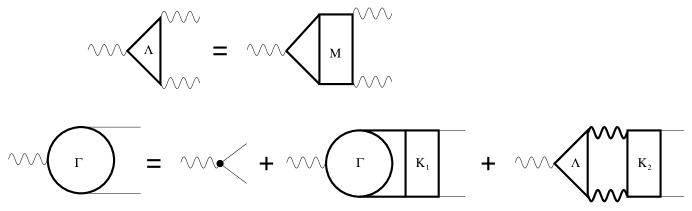
Figure 1: Schwinger-Dyson equations for the vertex function. Solid lines represent the $\mathcal{G}_{ij}(t,t^{\prime})$ propagator and heavy wiggly lines are the $\mathcal{D}(t,t^{\prime})$ propagator.

In our truncations of the Schwinger-Dyson equations, we will always replace the full three-point vertex function by the bare one in the equations for $x$ and $\mathcal{G}$ in the presence of external sources. Once this truncation is made, then for the problem we are addressing here (the approximate time evolution of $N$ quantum anharmonic oscillators) one never needs any of the $N$ point functions beyond the 1 and 2 point function equations. What will distinguish a further approximation we will call the DDSA is that we will also further approximate the $\chi$ propagator to be that of the LOLN approximation.

By making this bare vertex approximation in the equations for the one- and two-point Green functions, we have not relinquished our ability to calculate in this approximation all the higher connected Green functions. These are obtainable by further functional differentiation of the effective action. In particular if we wanted to use linear response theory (the Kubo formula) to obtain the electrical conductivity for a QED plasma, one would functionally differentiate the equation for the inverse two-point for the electron function with respect to $A_{\mu}$. In our problem the photon is replaced by the composite field $\chi$, and the electron by $x_{i}$.

Because of recent interest in studying plasma conductivity in both QED and QCD, we will spend extra time on comparing the equations obtained for the vertex function in the three approximations considered here. In conductivity calculations, it is necessary to sum all the ladder graphs in the equation for the vertex function to get good results for dilute plasmas. We will find that in NLOLN the vertex function is not an integral equation but is rather the sum of a few diagrams whereas the other two approximations lead to integral equations that sum an infinite number of diagrams. Another issue is in preserving Ward identities. One of the reasons the large-$N$ expansion was so interesting is that it is a complete reexpansion of the field theory which preserves Ward identities at each order. The QED plasma conductivity problem people ref:emil became interested in the DDSA because it exactly obeyed the Ward identities, whereas the BVA approximation violates Ward identities at order $1/N^{2}$. It is for this reasons we thought it appropriate to study the DDSA approximation, even though it violated energy conservation already at order $1/N$, hoping that at least at large $N$ it would be numerically accurate and satisfy Ward identities in QED applications.

The exact formula for the energy is given by:

$$E/N=\frac{1}{2}\left\langle\sum_{i}\left\{\hat{\dot{x}}_{i}^{2}(t)+\hat{\chi}(t)\,\hat{x}_{i}^{2}(t)-r_{0}^{2}\hat{\chi}(t)-\hat{\chi}^{2}(t)/g\right\}\right\rangle\>.$$ (38)

When $x_{i}(t)=\langle\hat{x}_{i}(t)\rangle=0$ and $\dot{x}_{i}(t)=0$, one obtains:

$$E/N =\frac{1}{2}\sum_{i}\biggl{\{}\left.\frac{\partial^{2}\,\mathcal{G}(t,t^{\prime})/i}{\partial t\,\partial t^{\prime}}\right|_{t^{\prime}=t}+\chi(t)\,\mathcal{G}(t,t)/i-r_{0}^{2}\chi(t)-\frac{1}{g}\left[\chi^{2}(t)+\frac{1}{N}\mathcal{D}(t,t)/i\right]$$

$$\qquad+\frac{1}{N}\sum_{ijk}\int_{\mathcal{C}}\mathrm{d}t_{1}\!\!\int_{\mathcal{C}}\mathrm{d}t_{2}\!\!\int_{\mathcal{C}}\mathrm{d}t_{3}\,\mathcal{D}(t_{1},t_{2})\,\mathcal{G}_{ij}(t_{1},t)\,\mathcal{G}_{ik}(t,t_{1})\,\Gamma_{jk}(t_{1},t_{3},t_{2})\biggr{\}}\>,$$ (39)

where $\Gamma_{jk}(t_{1},t_{3},t_{2})$ is the full vertex function given in Eq. (37).

IV Effective action for two-particle irreducible graphs

Since the approximations we are going to consider have a simple interpretation in terms of keeping a particular 2-PI vacuum graph in the generating functional of the 2-PI graphs, we would like to review this formalism following the approach of Cornwall, Jackiw, and Tomboulis (CJT)ref:CJT .

The first Legendre transform of the generating functional $W[j]$ of connected Green functions is widely known and used and is called the “effective action.” The higher Legendre transforms (second, third, etc.) were introduced by De Dominicis and Martinref:DM in quantum statistics. Dahmen and Jona-Lasinioref:DJL , and later Visil’ev and Kazanskiiref:VK , extended these ideas to quantum field theory. These methods were then used by Cornwall, Jackiw, and Tomboulis to discuss dynamical symmetry breaking in Hartree type approximations which later led to the second Legendre transformation formalism being called the CJT formalism. These higher order Legendre transformed actions have the advantage of being able to treat higher order Green functions on the same footing as the coordinates.

We will first summarize the general results of that paper before proceeding to the specific approximations we consider in this paper. The method of CJT is to introduce one- and two-body sources for the coordinates $x_{\alpha}(t)$ and the Green functions $\mathcal{G}_{\alpha,\beta}(t,t^{\prime})$ in the action, and then make a Legendre transformation to the one- and two-point functions. The resulting action, as a function of $x$ and $\mathcal{G}$, contains a term which is the sum of all two-particle irreducible vacuum graphs. This term can be written using the vertices of the interaction and $\mathcal{G}$. We use the extended notation for the coordinates and one-body sources, given in Eq. (12).

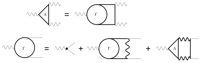
Figure 2: The vertex function for the BVA. The top figure represents Eq. (57) and the bottom figure represents Eq. (58). Solid lines represent the $\mathcal{G}_{ij}(t,t^{\prime})$ propagator and heavy wiggly lines are the $\mathcal{D}(t,t^{\prime})$ propagator.

Thus, the generating functional $Z[j,k]$ for the CJT action is given by:

$$Z[j,k]=e^{iNW[j,k]}=\prod_{\alpha=0}^{N}\int\mathrm{d}x_{\alpha}\,\exp\left\{iNS_{N}[x;j,k]\right\}\>,$$

with

$$S_{N}[x;j,k]=S_{\text{class}}[x]+\sum_{\alpha}\int_{\mathcal{C}}\mathrm{d}t\,x_{\alpha}(t)\,j_{\alpha}(t)+\frac{1}{2}\sum_{\alpha,\beta}\int_{\mathcal{C}}\mathrm{d}t\!\!\int_{\mathcal{C}}\mathrm{d}t^{\prime}\,x_{\alpha}(t)\,k_{\alpha,\beta}(t,t^{\prime})\,x_{\beta}(t^{\prime})\>,$$ (40)

where

$$S_{\text{class}}[x] =-\frac{1}{2}\sum_{\alpha,\beta}\int_{\mathcal{C}}\mathrm{d}t\!\!\int_{\mathcal{C}}\mathrm{d}t^{\prime}\,x_{\alpha}(t)\,\Delta_{\alpha,\beta}^{-1}[x](t,t^{\prime})\,x_{\beta}(t^{\prime})=S_{0}+S_{\text{int}}[x]\>,$$ (41)

$$S_{0} =-\frac{1}{2}\sum_{\alpha,\beta}\int_{\mathcal{C}}\mathrm{d}t\!\!\int_{\mathcal{C}}\mathrm{d}t^{\prime}\,x_{\alpha}(t)\,\Delta_{0\,\alpha,\beta}^{-1}(t,t^{\prime})\,x_{\beta}(t^{\prime})\>,$$ (42)

$$S_{\text{int}}[x] =-\frac{1}{2}\int_{\mathcal{C}}\mathrm{d}t\,\chi(t)\sum_{i}x_{i}^{2}(t)\>,$$ (43)

and where $\Delta_{0\,\alpha,\beta}^{-1}(t,t^{\prime})$ is given by:

$$\Delta_{0\,\alpha,\beta}^{-1}(t,t^{\prime}) =\begin{pmatrix}D^{-1}(t,t^{\prime})&0\\ 0&G_{0\,ij}^{-1}(t,t^{\prime})\end{pmatrix}\>,$$

$$G_{0\,ij}^{-1}(t,t^{\prime}) =\biggl{\{}\frac{\mathrm{d}^{2}}{\mathrm{d}t^{2}}\biggr{\}}\,\delta_{ij}\delta_{\mathcal{C}}(t,t^{\prime})\>.$$

with $D^{-1}(t,t^{\prime})$ given by Eq. (16). In this formalism, we have separated out an “interaction” term, Eq. (43), which depends on the coordinates $x_{\alpha}(t)$, from a bare Green function $G_{0\,ij}^{-1}(t,t^{\prime})$, which is independent of the coordinates $x_{\alpha}(t)$, in contrast to our previous definitions in Eq. (16). The term $r_{0}^{2}\chi(t)/2$ has been absorbed into the definition of the current $\tilde{J}(t)$ in Eq. (12).

The second Legendre transform of $W[j,k]$ is the CJT effective action:

$$\Gamma[x,\mathcal{G}]=W[j,k]-\sum_{\alpha}\int_{\mathcal{C}}\mathrm{d}t\,x_{\alpha}(t)\,j_{\alpha}(t)\\ +\frac{1}{2}\sum_{\alpha,\beta}\int_{\mathcal{C}}\mathrm{d}t\!\!\int_{\mathcal{C}}\mathrm{d}t^{\prime}\,k_{\alpha,\beta}(t,t^{\prime})\left\{x_{\alpha}(t)\,x_{\beta}(t^{\prime})+\mathcal{G}_{\alpha,\beta}(t,t^{\prime})\right\}$$

CJT showed that $\Gamma[x,\mathcal{G}]$ can be obtained as a series expansion in terms of 2-PI graphs. That is, introducing the functional operator,

$$G^{-1}_{\alpha,\beta}[x](t,t^{\prime}) =-\frac{\delta^{2}S_{0}[x]}{\delta x_{\alpha}(t)\,\delta x_{\beta}(t^{\prime})}$$

$$=\begin{pmatrix}D^{-1}(t,t^{\prime})&\bar{K}_{j}^{-1}[x](t,t^{\prime})\\ K_{i}^{-1}[x](t,t^{\prime})&G_{i,j}^{-1}[x](t,t^{\prime})\end{pmatrix}\>,$$ (44)

which is the same as the $G^{-1}_{\alpha,\beta}[x](t,t^{\prime})$ as defined in Eq. (17), one can write the effective action in the form:

$$\Gamma[x,\mathcal{G}]=S_{\text{class}}[x]+\frac{i}{2}\mathrm{Tr}\{\,\ln\,[\,\mathcal{G}^{-1}\,]\}\\ +\frac{i}{2}\mathrm{Tr}\{G^{-1}[x]\,\mathcal{G}-1\}+\Gamma_{2}[x,\mathcal{G}]\>.$$ (45)

The quantity $\Gamma_{2}[x,\mathcal{G}]$ has a simple graphical interpretation in terms of all the 2-PI vacuum graphs using vertices from the interaction term. The Hartree and leading order in large-$N$ approximation for the $x^{4}$ potential was obtained by CJT using a single two-loop vacuum graph in the $O(N)$ theory written in terms of only the coordinates $x_{i}$. Our strategy for obtaining a resummation of the large-$N$ approximation is to first rewrite the theory in terms of the composite field $\chi$, and the equivalent Lagrangian given in Eq. (9). Using these new variables, we then choose for $\Gamma_{2}[x,\mathcal{G}]$ the 2-PI graphs shown in Fig. 3, which is now written in terms of the full $\chi$ and $x$ propagators and the trilinear coupling $\chi(t)\,x_{i}^{2}(t)/2$.

V Bare Vertex Approximation

The bare vertex approximation (BVA) is obtained by setting the vertex function equal to its bare value in the exact equations for the one and two point functions. This is an energy conserving approximation which leads to integral equations for the three-$\chi$ vertex function as well as for the $x$-$x$-$\chi$ vertex function. The bare vertex approximation consists of making the replacement

$$\Gamma_{\alpha,\beta,\gamma}[x](t_{1},t_{2},t_{3})=f_{\alpha,\beta,\gamma}\,\delta_{\mathcal{C}}(t_{1},t_{2})\,\delta_{\mathcal{C}}(t_{1},t_{3})\>.$$ (46)

in the exact Schwinger-Dyson equations for the self-energies, Eqs. (28). This gives for the BVA:

$$\Pi(t,t^{\prime}) =\frac{i}{2N}\sum_{ij}\mathcal{G}_{ij}(t,t^{\prime})\,\mathcal{G}_{ji}(t^{\prime},t)\>,$$ (47)

$$\Omega_{i}(t,t^{\prime}) =\frac{i}{N}\,\sum_{j}\bar{\mathcal{K}}_{j}(t,t^{\prime})\,\mathcal{G}_{ji}(t,t^{\prime})\>,$$

$$\bar{\Omega}_{i}(t,t^{\prime}) =\frac{i}{N}\,\sum_{j}\mathcal{K}_{j}(t^{\prime},t)\,\mathcal{G}_{ji}(t^{\prime},t)\>,$$

$$\Sigma_{ij}(t,t^{\prime}) =\frac{i}{N}\,\bigl{\{}\bar{\mathcal{K}}_{i}(t,t^{\prime})\,\mathcal{K}_{j}(t^{\prime},t)+\mathcal{G}_{ij}(t,t^{\prime})\,\mathcal{D}(t^{\prime},t)\bigr{\}}\>,$$

where we have used the symmetry property, $\mathcal{G}_{ij}(t,t^{\prime})=\mathcal{G}_{ji}(t^{\prime},t)$ and $\mathcal{K}_{i}(t,t^{\prime})=\bar{\mathcal{K}}_{i}(t^{\prime},t)$. Thus we find $\bar{\Omega}_{i}(t,t^{\prime})=\Omega_{i}(t^{\prime},t)$. The self-energies (47) are then used in Eqs. (26) to find the one- and two-point functions. For the Green functions, we find:

$$\mathcal{G}_{\alpha,\beta}^{-1}(t,t^{\prime})=G_{\alpha,\beta}^{-1}(t,t^{\prime})+\Sigma_{\text{BVA}\,\alpha,\beta}(t,t^{\prime})\>,$$ (48)

with $\Sigma_{\text{BVA}\,\alpha,\beta}(t,t^{\prime})$ given by Eq. (47). The inversion of Eq. (48) is given by Eq. (29), which is a set of four coupled integral equations for the four BVA Green functions, which must be solved simultaneously.

From Eqs. (22) and (23), the equations of motion for $x_{i}(t)$ and the gap equation for $\chi(t)$ is then given by:

$$\biggl{\{}\frac{\mathrm{d}^{2}}{\mathrm{d}t^{2}}+\chi(t)\biggr{\}}\,x_{i}(t)+\frac{1}{N}\mathcal{K}_{i}(t,t)/i=0\>,$$ (49)

$$\chi(t)=\frac{g}{2}\biggl{\{}\sum_{i}\biggl{[}x_{i}^{2}(t)+\frac{1}{N}\mathcal{G}_{ii}(t,t)/i\biggr{]}-r_{0}^{2}\biggr{\}}\>.$$ (50)

For the quantum roll, we further set $x_{i}(t)=0$. This means that $\mathcal{K}_{i}(t,t)=\bar{\mathcal{K}}_{i}(t,t)=0$, so that $G_{\alpha\beta}(t,t^{\prime})$ is diagonal, and results in the following set of equations for the Green functions:

$$\mathcal{D}(t,t^{\prime}) =D(t,t^{\prime})$$

$$\!\!\!\!\!\!\!\!\!\!\!\!-\int_{\mathcal{C}}\mathrm{d}t_{1}\!\!\int_{\mathcal{C}}\mathrm{d}t_{2}\,D(t,t_{1})\,\Pi(t_{1},t_{2})\,\mathcal{D}(t_{2},t^{\prime})\>,$$ (51)

$$\mathcal{G}_{ij}(t,t^{\prime}) =G_{ij}(t,t^{\prime})$$

$$\!\!\!\!\!\!\!\!\!\!\!\!-\sum_{kl}\int_{\mathcal{C}}\mathrm{d}t_{1}\!\!\int_{\mathcal{C}}\mathrm{d}t_{2}\,G_{ik}(t,t_{1})\,\Sigma_{kl}(t_{1},t_{2})\,\mathcal{G}_{lj}(t_{2},t^{\prime})\>,$$ (52)

where

$$\Pi(t,t^{\prime}) =\frac{i}{2N}\sum_{ij}\mathcal{G}_{ij}(t,t^{\prime})\,\mathcal{G}_{ji}(t^{\prime},t)\>,$$

$$\Sigma_{ij}(t,t^{\prime}) =\frac{i}{N}\,\mathcal{G}_{ij}(t,t^{\prime})\,\mathcal{D}(t^{\prime},t)\>.$$ (53)

The gap equation for $\chi(t)$ becomes:

$$\chi(t)=\frac{g}{2}\biggl{\{}\frac{1}{N}\sum_{i}\mathcal{G}_{ii}(t,t)/i-r_{0}^{2}\biggr{\}}\>.$$ (54)

In addition, for this case, the initial conditions imply that we can take $G_{ij}(t,t^{\prime})$ and $\mathcal{G}_{ij}(t,t^{\prime})$ to be diagonal, which greatly simplify the integral equations. The BVA for the quantum roll requires that we solve equations (51), (52), (53), and (54) simultaneously using the numerical methods described in refs. ref:MDC and ref:BMIM .

Because of the interest in using the BVA approximation in QED (and QCD) plasma conductivity problems, we will discuss the integral equation one obtains for the vertex function in what follows. It was precisely because this approximation gives the sum of the graphs used in non-relativistic plasmas (see Fig. 2) in conductivity calculations which gave both accurate results as well as giving physical answers that initially interested us in this approximation.

The three-point vertex functions for the BVA are given by functional differentiation of the inverse two point functions:

$$\Lambda(t_{1},t_{2},t_{3}) \equiv\Gamma_{000}(t_{1},t_{2},t_{3})=\frac{\delta\,\mathcal{D}^{-1}(t_{1},t_{2})}{\delta\chi(t_{3})}$$ (55)

$$\Gamma_{ij}(t_{1},t_{2},t_{3}) \equiv\Gamma_{ij0}(t_{1},t_{2},t_{3})=\frac{\delta\,\mathcal{G}_{ij}^{-1}(t_{1},t_{2})}{\delta\chi(t_{3})}\>,$$ (56)

and obtain the coupled integral equations:

$$\Lambda(t_{1},t_{2},t_{3})=-\frac{i}{N}\int_{\mathcal{C}}\mathrm{d}t_{4}\int_{\mathcal{C}}\mathrm{d}t_{5}\sum_{ijkl}\mathcal{G}_{ik}(t_{1},t_{4})\,\Gamma_{kl}(t_{4},t_{5},t_{3})\,\mathcal{G}_{lj}(t_{5},t_{2})\,\mathcal{G}_{ji}(t_{2},t_{1})$$ (57)

and

$$\Gamma_{ij}(t_{1},t_{2},t_{3})=\delta_{ij}\,\delta_{\mathcal{C}}(t_{1},t_{2})\,\delta_{\mathcal{C}}(t_{1},t_{3})\\ -\int_{\mathcal{C}}\mathrm{d}t_{4}\int_{\mathcal{C}}\mathrm{d}t_{5}\biggl{\{}\sum_{kl}\mathcal{G}_{ik}(t_{1},t_{4})\,\Gamma_{kl}(t_{4},t_{5},t_{3})\,\mathcal{G}_{lj}(t_{5},t_{2})\,\mathcal{D}(t_{2},t_{1})+\mathcal{G}_{ij}(t_{1},t_{2})\mathcal{D}(t_{2},t_{4})\,\Lambda(t_{4},t_{5},t_{3})\,\mathcal{D}(t_{5},t_{1})\biggr{\}}\>.$$ (58)

This is shown diagrammatically in Fig. 2. Looking at the diagrams, if we iterate these equations, we sum all the “rainbow” diagrams. As advertised, comparing these graphs with those shown in Fig. 1, $\mathcal{K}_{1}$ is approximated in the BVA by $\chi$ exchange and $\mathcal{K}_{2}$ by $x$ exchange in the $t$-channel.

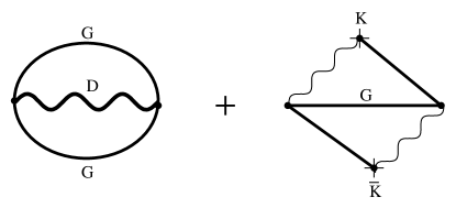
Figure 3: Vacuum graphs contributing to the 2PI part of the effective action $\Gamma_{2}[\mathcal{G}]$. Solid lines represent the $\mathcal{G}_{ij}(t,t^{\prime})$ propagator, the wiggly to solid lines represent the $\mathcal{K}_{i}(t,t^{\prime})$ and $\bar{\mathcal{K}}_{i}(t,t^{\prime})$ propagator, and wiggly lines are the $\mathcal{D}(t,t^{\prime})$ propagator.

Let us show that this approximation is easy to obtain from the CJT formalism once we treat $\mathcal{G}$ and $\mathcal{D}$ and $\mathcal{K}$ on exactly the same footing. We choose for our approximation to $\Gamma_{2}[\mathcal{G}]$ the 2-PI graphs shown in Fig. 3. This gives:

$$\Gamma_{2}[\mathcal{G}]=-\frac{1}{4N}\sum_{ij}\int_{\mathcal{C}}\mathrm{d}t_{1}\int_{\mathcal{C}}\mathrm{d}t_{2}\,\mathcal{D}(t_{1},t_{2})\,\mathcal{G}_{ij}(t_{1},t_{2})\,\mathcal{G}_{ji}(t_{2},t_{1})-\frac{1}{2N}\sum_{ij}\int_{\mathcal{C}}\mathrm{d}t_{1}\int_{\mathcal{C}}\mathrm{d}t_{2}\,\bar{\mathcal{K}}_{i}(t_{1},t_{2})\,\mathcal{G}_{ij}(t_{1},t_{2})\,\mathcal{K}_{j}(t_{2},t_{1})\>.$$ (59)

Since the $\mathcal{D}$ propagator sums the contact term plus all the polarization bubbles $\Pi$ of the original quartic interaction $gx^{4}$, if we reexpand $\mathcal{D}$ in a power series in $\Pi$ then the first two terms in the series give the graphs used in the approximation ofref:Hu andref:berges . The CJT action is given by Eq. (45). The stationary condition for $\mathcal{G}_{\alpha,\beta}(t,t^{\prime})$ gives:

$$\frac{\delta\Gamma[x,\mathcal{G}]}{\delta\mathcal{G}_{\alpha\beta}}=\frac{i}{2}\left\{G^{-1}_{\alpha\beta}[x]-\mathcal{G}^{-1}_{\alpha\beta}\right\}+\frac{\delta\Gamma_{2}[\mathcal{G}]}{\delta\mathcal{G}_{\alpha\beta}}=0\>,$$

or

$$\mathcal{G}_{\alpha,\beta}^{-1}(t,t^{\prime})=G_{\alpha,\beta}^{-1}(t,t^{\prime})+\Sigma_{\text{BVA}\,\alpha,\beta}[\mathcal{G}](t,t^{\prime})\>,$$

where:

$$\Sigma_{\text{BVA}\,\alpha,\beta}[\mathcal{G}](t,t^{\prime})=-2i\,\frac{\delta\Gamma_{2}[\mathcal{G}]}{\delta\mathcal{G}_{\alpha\beta}(t,t^{\prime})}\>.$$ (60)

Carrying out the derivatives of $\Gamma_{2}[\mathcal{G}]$ given in Eq. (59), we find that $\Sigma_{\text{BVA}\,\alpha,\beta}(t,t^{\prime})$ is exactly the same as found in Eq. (47) using the Schwinger-Dyson equations in the BVA approximation. The stationary condition for $x_{\alpha}$ also gives the same equations of motion for $x_{i}(t)$ and gap equation for $\chi(t)$ as found in Eqs. (49) and (50) using the Schwinger-Dyson equations in the BVA. Thus we conclude that the CJT action, as given in Eqs. (45) and (59), gives exactly the same set of equations as in the Schwinger-Dyson BVA truncation.

The energy for the BVA is obtained from (39) by using (46) for the vertex function. We find:

$$E/N =\frac{1}{2}\sum_{i}\biggl{\{}\left.\frac{\partial^{2}\,\mathcal{G}(t,t^{\prime})/i}{\partial t\,\partial t^{\prime}}\right|_{t^{\prime}=t}+\chi(t)\,\mathcal{G}(t,t)/i-r_{0}^{2}\chi(t)-\frac{1}{g}\left[\chi^{2}(t)+\frac{1}{N}\mathcal{D}(t,t)/i\right]$$

$$\quad+\frac{1}{N}\sum_{ij}\int_{\mathcal{C}}\mathrm{d}t_{1}\,\mathcal{D}(t_{1},t)\mathcal{G}_{ij}(t_{1},t)\mathcal{G}_{ji}(t,t_{1})\biggr{\}}\>.$$ (61)

where, for our case, we have set $x_{i}(t)=\dot{x}_{i}(t)=0$. Since the BVA equations are derived from an effective action, energy is conserved.

VI Dynamical Debye Screening Approximation

In plasma studies of the electric conductivity of fully ionized plasmas ref:plasma1 ; ref:plasma2 , it was found that in order to correctly determine the conductivity it was necessary to have an approximation where the photon propagator included the effects of dynamical Debye screening in the random phase approximation. This improved propagator was then used in a scattering kernel in the kinetic equations. In our model, the $\chi$ field plays the roll of the photon in the dynamics of the $x_{i}$ oscillators. The lowest approximation that includes the polarization effects in $\mathcal{D}$ is precisely the leading order in large-$N$ approximation to $\mathcal{D}$, namely $\mathcal{D}_{0}$ (see Eq. 69) which is discussed below in our derivation of the NLOLN approximation . The leading order in large-$N$ approximation is similar in spirit to the random phase approximation. The equation for $\mathcal{D}^{-1}(t,t^{\prime})$ in leading order in large-$N$ is given by:

$$\mathcal{D}_{0}^{-1}(t,t^{\prime})=-\frac{1}{g}\delta_{\mathcal{C}}(t,t^{\prime})+\Pi_{0}(t,t^{\prime})\>,$$ (62)

where

$$\Pi_{0}(t,t^{\prime})=\frac{i}{2N}\,\sum_{i,j}G_{ij}(t,t^{\prime})\,G_{ji}(t^{\prime},t)\\ +\sum_{i,j}\,x_{i}(t)\,G_{ij}(t,t^{\prime})\,x_{j}(t^{\prime})\>.$$

In the QED plasma problem, the $\chi$ propagator becomes the photon propagator and the delta function in $\mathcal{D}_{0}$ is replaced by the bare photon propagator. It is the bubble in $\Pi_{0}$ that leads to the Debye screening of the photon. It is because of our interest in QED that we call this approximation the DDSA.

Let us now specialize to the case when $x_{i}(t)=0$. The equation for the full $x$ propagator ${\cal G}$ is:

$$\mathcal{G}_{ij}(t,t^{\prime})=G_{ij}(t,t^{\prime})\\ -\sum_{k,l}\int_{\mathcal{C}}\!{\rm d}t_{1}\!\!\int_{\mathcal{C}}\!{\rm d}t_{2}\,G_{ik}(t,t_{1})\,\Sigma_{kl}(t_{1},t_{2})\,\mathcal{G}_{lj}(t_{2},t^{\prime})\>,$$ (63)

with the self energy depending on the full ${\cal G}$ and the leading order in $1/N$ approximation to $\mathcal{D}$ given by Eq. (62):

$$\Sigma_{kl}(t,t^{\prime})=\frac{i}{N}\,\mathcal{G}_{kl}(t,t^{\prime})\,D(t,t^{\prime})\>.$$ (64)

The gap equation is:

$$\chi(t)=\frac{g}{2}\ \left\{\sum_{i}\frac{1}{N}\mathcal{G}_{ii}(t,t)/i-r_{0}^{2}\right\}\>.$$ (65)

There is a nontrivial vertex function in this approximation given by:

$$\Gamma_{ij}(t_{1},t_{2},t_{3}) =\frac{\delta\mathcal{G}^{-1}_{ij}[\chi](t_{1},t_{2})}{\delta\chi(t_{3})}$$

$$=\delta_{\mathcal{C}}(t_{1},t_{2})\delta_{\mathcal{C}}(t_{3},t_{2})\delta_{ij}-\sum_{kl}\int_{\mathcal{C}}\mathrm{d}t_{4}\int_{\mathcal{C}}\mathrm{d}t_{5}\,\Gamma_{kl}(t_{4},t_{5},t_{3})\,\mathcal{G}_{ki}(t_{4},t_{1})\,D(t_{1},t_{2})\,\mathcal{G}_{jl}(t_{2},t_{5})$$

$$\qquad-\int_{\mathcal{C}}\mathrm{d}t_{4}\int_{\mathcal{C}}\mathrm{d}t_{5}\,\Lambda(t_{4},t_{5},t_{3})\,D(t_{4},t_{1})\,\mathcal{G}_{ij}(t_{1},t_{2})\,D(t_{2},t_{5})\>.$$ (66)

This equation can be obtained from the exact integral equation for $\Gamma$ shown pictorially in Fig. 1 by making two approximations. The first is to approximate the exact three-$\chi$ vertex function by the triangle graph, which is the leading term in the $1/N$ expansion of this function. The second is to replace the scattering kernels, $K_{1}$ and $K_{2}$ by single particle exchange in the t-channel. The reason for our studying this approximation is that, the same approximation made in QED can be shown to be the lowest order resummation scheme that preserves Ward identities (ref:emil ).

The DDSA approximation can be derived from an effective action by modifying slightly the approach of Cornwall, Jackiw and Tomboulis (CJT)ref:CJT . The discussion that follows here is due to Emil Mottola and Luis Bettencourtref:emil . Thinking of the fields $x$ and $\chi$ as part of an $N+1$ component field, and considering the case that $\langle\hat{x}(t)\rangle=0$ where there is no mixed propagator, one can write a CJT like action for the generating functional of the twice Legendre transformed effective action as:

$$\Gamma[\chi,\mathcal{G},\mathcal{D}]=S_{\text{class}}[\chi]+\frac{i}{2}\mathrm{Tr}\{\,\ln\,[\,\mathcal{D}^{-1}\,]\}\\ +\frac{i}{2}\mathrm{Tr}\{\,\ln\,[\,\mathcal{G}^{-1}\,]\}+\frac{i}{2}\mathrm{Tr}\{\mathcal{D}_{0}^{-1}\,\mathcal{D}+G^{-1}[\chi]\,\mathcal{G}-1\}+\Gamma_{2}[\mathcal{G}]\>.$$ (67)

here $G^{-1}(t,t^{\prime})$ is defined by (16) and $\mathcal{D}_{0}(t,t^{\prime})$ by Eq. (62). $\mathcal{D}_{0}(t,t^{\prime})$ is considered an external parameter, and is not varied to obtain the equations of motion. In the DDSA, the 2-PI contribution to the action, $\Gamma_{2}[\mathcal{G}]$, for the case when $x_{i}(t)=0$, is given by Eq. (59) with $\mathcal{D}(t,t^{\prime})$ set equal to its LOLN value $\mathcal{D}_{0}(t,t^{\prime})$:

$$\Gamma_{2}[\mathcal{G}]=\\ -\frac{1}{4N}\sum_{ij}\int_{\mathcal{C}}\mathrm{d}t_{1}\int_{\mathcal{C}}\mathrm{d}t_{2}\,\mathcal{D}_{0}(t_{1},t_{2})\,\mathcal{G}_{ij}(t_{1},t_{2})\,\mathcal{G}_{ji}(t_{2},t_{1})\>.$$ (68)

By varying the action (67), we reproduce Eqs. (63) and (65). Although there is an effective action for the DDSA approximation, since $\mathcal{D}_{0}$ is treated as an external time-dependent propagator, energy conservation is violated at order $1/N$. At modest $N$ we will find that this causes this approximation to become inaccurate after several oscillations. However, it is more accurate at these modest values of $N$ than the LOLN approximation, as well avoiding the unboundedness of the NLOLN approximation we discuss next.

VII The large-$N$ approximation

The large-$N$ expansion is obtained from Eq. (13) by first integrating over all the $x_{i}$ and then evaluating the remaining functional integral over $\chi$ by steepest descent. The effective action, as a power series in $1/N$, is obtained from the first Legendre transform of the generating functional. In a previous paperref:ctpN , we obtained equations for the next to leading order large-$N$ approximation (NLOLN) to the action, and gave numerical results for the quantum roll. For completeness, we review those equations here. To order $1/N$, we obtain:

$$\Gamma_{\text{Large-N}}[x]=S_{\text{class}}[x]\\ +\int_{\mathcal{C}}\mathrm{d}t\,\biggl{\{}\frac{i}{2}\sum_{i}\,\ln\,[G_{ii}^{-1}(t,t)]+\frac{i}{2N}\ln[\mathcal{D}^{-1}_{0}(t,t)]\biggr{\}}\>,$$

where $S_{\text{class}}[x]$ is given by Eq. (41), and $\mathcal{D}^{-1}_{0}(t,t^{\prime})$ is the inverse propagators for $\chi$ in lowest order in the $1/N$ expansion, given by

$$\mathcal{D}^{-1}_{0}(t,t^{\prime})=D^{-1}(t,t^{\prime})+\Pi_{0}(t,t^{\prime})\>,$$ (69)

with

$$\Pi_{0}(t,t^{\prime}) =\frac{i}{2N}\,\sum_{i,j}G_{ij}(t,t^{\prime})\,G_{ji}(t^{\prime},t)$$

$$-\sum_{i,j}\,x_{i}(t)\,G_{ij}(t,t^{\prime})\,x_{j}(t^{\prime})\>.$$ (70)

Here $D^{-1}(t,t^{\prime})$ and $G^{-1}_{ij}(t,t^{\prime})$ are the same as Eqs. (16) that we defined earlier.

The equations of motion for the classical fields $x_{i}(t)$, to next to leading order in $1/N$, are given by:

$$\left\{\frac{{\rm d}^{2}}{{\rm d}t^{2}}+\chi(t)\right\}x_{i}(t)\\ +i\,\sum_{j}\int_{\mathcal{C}}{\rm d}t^{\prime}\,G_{ij}(t,t^{\prime})\,\mathcal{D}_{0}(t,t^{\prime})\,x_{j}(t^{\prime})=0\>,$$ (71)

with the gap equation for $\chi(t)$ given by

$$\chi(t)=\frac{g}{2}\left\{\sum_{i}\left(x_{i}^{2}(t)+\frac{1}{N}\sum_{i}\mathcal{G}^{(2)}_{ii}(t,t)/i\right)-r_{0}^{2}\right\}\>,$$ (72)

and where the second order $x_{i}$ propagator $\mathcal{G}^{(2)}_{ij}(t,t)$ and self energy $\Sigma_{ij}(t,t^{\prime})$ to order $1/N$ is given by:

$$\mathcal{G}^{(2)}_{ij}(t,t^{\prime})=G_{ij}(t,t^{\prime})\\ -\sum_{k,l}\int_{\mathcal{C}}{\rm d}t_{1}\!\!\int_{\mathcal{C}}{\rm d}t_{2}\,G_{ik}(t,t_{1})\,\Sigma_{kl}(t_{1},t_{2})\,G_{lj}(t_{2},t^{\prime})\>,$$ (73)

where

$$\Sigma_{ij}(t,t^{\prime})=\frac{i}{N}\,G_{ij}(t,t^{\prime})\,\mathcal{D}_{0}(t,t^{\prime})-x_{i}(t)\,\mathcal{D}_{0}(t,t^{\prime})\,x_{j}(t^{\prime})\>.$$

We see here that the equation for $\mathcal{G}$ is the expansion of the BVA equation in a series of $1/N$, truncated at first order.

Let us now specialize to the case of the quantum roll problem where $x_{i}(t)=0$. In that case the two point inverse propagator for the $x$ field is

$$\mathcal{G}^{-1}_{ij}[\chi](t_{1},t_{2}) =\frac{\delta^{2}\Gamma_{\text{Large-N}}[x,\chi]}{\delta x_{i}(t_{1})\,\delta x_{j}(t_{2})}$$

$$=G^{-1}_{ij}[\chi](t_{1},t_{2})+\Sigma_{ij}[\chi](t_{1},t_{2})\>,$$

with

$$\Sigma_{ij}[\chi](t,t^{\prime})=\frac{i}{N}\,G_{ij}(t,t^{\prime})\,\mathcal{D}_{0}(t,t^{\prime})$$

However it is $\mathcal{G}^{(2)}_{ij}(t,t^{\prime})$ which enters into Eq. (72) and not $\mathcal{G}_{ij}(t,t^{\prime})$. Thus the solution for $\mathcal{G}_{ij}(t,t^{\prime})$, which we might interpret as $\langle\hat{x}_{i}(t)\hat{x}_{j}(t^{\prime})\rangle$, does not enter into the dynamics of the solution! This $\mathcal{G}_{ii}(t,t)$ is positive definite, but quickly blows up.

The vertex function $\Gamma_{ij}(t_{1},t_{2},t_{3})$ is given by:

$$\Gamma_{ij}(t_{1},t_{2},t_{3}) =\frac{\delta\mathcal{G}^{-1}_{ij}[\chi](t_{1},t_{2})}{\delta\chi(t_{3})}$$ (74)

$$=\delta_{\mathcal{C}}(t_{1},t_{2})\delta_{\mathcal{C}}(t_{2},t_{3})\delta_{ij}-\frac{i}{N}\,G_{ij}(t_{1},t_{3})\,G_{ji}(t_{3},t_{2})\,\mathcal{D}_{0}(t_{2},t_{1})$$

$$\qquad-\frac{i}{N}\,\int_{\mathcal{C}}\mathrm{d}t_{4}\!\!\int_{\mathcal{C}}\mathrm{d}t_{5}\,G_{ij}(t_{1},t_{2})\,\mathcal{D}_{0}(t_{1},t_{4})\Lambda_{0}(t_{4},t_{5},t_{3})\,\mathcal{D}_{0}(t_{5},t_{2})\>,$$

where the lowest order in $1/N$ 3-$\chi$ vertex is given by

$$\Lambda_{0}(t_{4},t_{5},t_{3}) =\frac{\delta\mathcal{D}^{-1}_{0}(t_{4},t_{5})}{\delta\chi(t_{3})}$$

$$=-\frac{i}{N}\sum_{ijk}G_{ij}(t_{4},t_{3})\,G_{kl}(t_{3},t_{5})\,G_{li}(t_{5},t_{4})\>.$$

We immediately see that this is not an integral equation but again, is the lowest order in $1/N$ contribution to Eq. (57).

The inverse $\chi$ propagator gets $1/N$ corrections which are of two types, one is a self energy correction to the $x$ propagator and the other is a new three loop graph containing two lowest order $\chi$ propagators. We find

$$\mathcal{D}^{-1}(1,2) =\frac{\delta^{2}\Gamma_{\text{Large-N}}[x,\chi]}{\delta\chi(t_{1})\,\delta\chi(t_{2})}$$

$$=-\frac{1}{g}\delta_{\mathcal{C}}(1,2)-\Pi_{0}(1,2)-\sum_{ijkl}\int_{\mathcal{C}}\mathrm{d}t_{3}\!\!\int_{\mathcal{C}}\mathrm{d}t_{4}\,G_{ij}(t_{1},t_{3})\,\Sigma_{jk}(t_{3},t_{4})\,G_{kl}(t_{4},t_{2})\,G_{li}(t_{2},t_{1})$$

$$\qquad\qquad+\int_{\mathcal{C}}\mathrm{d}t_{3}\!\!\int_{\mathcal{C}}\mathrm{d}t_{4}\!\!\int_{\mathcal{C}}\mathrm{d}t_{5}\!\!\int_{\mathcal{C}}\mathrm{d}t_{6}\,\Lambda_{0}(t_{4},t_{1},t_{3})\,\mathcal{D}_{0}(t_{3},t_{5})\,\Lambda_{0}(t_{5},t_{2},t_{6})\,\mathcal{D}_{0}(t_{6},t_{4})\>.$$

The last term in this equation is a $1/N$ correction to the vertex function. However, it is $\mathcal{D}_{0}$ and not $\mathcal{D}$ which enters Eq. (73), so that the BVA and the $1/N$ expansion will differ only by terms of order $1/N^{2}$. The BVA approximation treats $x$ and $\chi$ on exactly the same footing, whereas the large-$N$ expansion treats $x$ exactly, but then expands in loops of $\chi$. So at order $1/N^{2}$, the large-$N$ approximation will contain graphs omitted from the BVA approximation, and vice-versa.

VIII Results and Conclusions

In this section we present the results of exact numerical simulations of the quantum roll, using initial conditions described in our previous paper on the large-$N$ approximationref:paper1 . We choose as our dimensional mass scale the second derivative of $U(r)$ at the minimum of the effective one dimensional potential $U(r)$. This mass scale was chosen to have value $M^{2}=2$. In terms of this mass scale, the coupling constant as well as the rescaled $r_{0}$ are of order one for all $N$. The exact manner in which $g$ and $r_{0}$ runs with $N$ is described in ref. ref:paper1 .

Figure 4: Plot of $\langle x^{2}(t)\rangle$ as a function of $t$, comparing the bare vertex, the dynamic Debye screening, and the large-$N$ approximations to the exact solution, for $N=3$.

Figure 5: Plot of $\langle x^{2}(t)\rangle$ as a function of $t$, comparing the bare vertex, the dynamic Debye screening, and the large-$N$ approximations to the exact solution, for $N=10$.

Figure 6: Plot of $\langle x^{2}(t)\rangle$ as a function of $t$, comparing the bare vertex, the dynamic Debye screening, and the large-$N$ approximations to the exact solution, for $N=21$.

Figure 7: Plot of $\langle\chi(t)\rangle$ as a function of $t$, comparing the bare vertex, the dynamic Debye screening, and the large-$N$ approximations to the exact solution, for $N=3$.

Figure 8: Plot of $\langle\chi(t)\rangle$ as a function of $t$, comparing the bare vertex, the dynamic Debye screening, and the large-$N$ approximations to the exact solution, for $N=21$.

Figure 9: Plot of $\langle\chi^{2}(t)\rangle$ as a function of $t$, comparing the bare vertex, the dynamic Debye screening, and the large-$N$ approximations to the exact solution for $N=3$.

Figure 10: Plot of $\langle\chi^{2}(t)\rangle$ as a function of $t$, comparing the bare vertex, the dynamic Debye screening, and the large-$N$ approximations to the exact solution for $N=10$.

Figure 11: Plot of $\langle\chi^{2}(t)\rangle$ as a function of $t$, comparing the bare vertex approximation to the exact solution for $N=21$.

Figure 12: Plot of various contributions to the energy for the bare vertex approximation as a function of $t$ for $N=10$.

As $N\rightarrow\infty$ the Hartree and leading order large-$N$ approximation become exact and an initially gaussian wave packet remains gaussian with width equal to $\langle x^{2}(t)\rangle$ oscillating in a known manner. At modest $N$, $10<N<20$ an initially Gaussian wave function develops a large number of nodes and so the wave function even at modest times is of the form Gaussian time a high order polynomial. In spite of this, $\langle x^{2}(t)\rangle$ shows rather simple behavior. It oscillates with a constant amplitude for a reasonable period of time with an envelope that oscillates with a much longer time constant which increases with $N$. The Hartree and leading order large-$N$ approximations just oscillate with fixed amplitude. The NLOLN blows up in this regime. BVA attempts to track the contraction of the envelope but then contracts to a fixed point. The DDSA violates energy conservation at order $1/N$ so it becomes numerically inaccurate when $1/N$ effects become important which is at a time $t\propto N$. Both BVA and DDSA do however stay bounded and positive definite during the time period of our numerical simulations. Higher order correlation functions show more complicated behavior and the approximations presented here are only accurate for a few oscillations in the regime $3<N<20$ consistent with the increasingly complicated evolving structure of the wave function.

In Figs. 4 through 6, we show the results for $\langle x^{2}(t)\rangle$ as a function of $t$, comparing the bare vertex, the dynamic Debye screening, and the large-$N$ approximations to the exact solution, for $N=3$, $10$, and $21$. In Figs. 7 to 8, we show the same results for $\langle\chi(t)\rangle$ as a function of $t$, and in Figs. 9 through 11, we give the results for $\langle\chi^{2}(t)$ [For detailed views of these figures in color, see our web site at: http://www.theory.unh.edu/resum].

In our previous studiesref:paper1 of the large-$N$ approximation, we found that the next to leading order large-$N$ approximation had the feature that the effective potential was not defined at small $x$ for $N\leq 20$, for our parameter set, and it was not until $N$ was greater than about $20$ that the large-$N$ expansion produced bounded values for $\langle x^{2}(t)\rangle$. This result is reproduced here. For the limit $N\rightarrow\infty$ the quantity $\langle x^{2}(t)\rangle$ corresponds to harmonic oscillations. At finite $N$, however, the exact solution for $N\geq 21$ has the property that the envelope of these oscillations contracts. As noted in the figures, only the bare vertex approximation attempts to follow this contraction. At $N=21$, the BVA is accurate up to a $t\approx 130$ before overshooting and then oscillating about a fixed point. This fixed point behavior shows that this approximation still neglects some important quantum phase information present in the exact solution.

In contrast to the NLOLN approximation, which breaks down for $N<21$, both the BVA and the DDSA have the feature that $\langle x^{2}(t)\rangle$ remains positive definite, as well as being bounded at all $N$. This is true for all the expectation values that contribute to the energy. This conclusion is purely based on numerical evidence. We do not have a proof that this approximation corresponds to a positive definite probability distribution. However, all the moments we have studied (a total of five, as shown in Fig. 12), are all bounded.

The DDSA is more accurate than the second order large-$N$ approximation for $N$ less that $20$, but for $N$ greater than $20$, the reverse becomes true. However, neither approximation captures the true nonlinear shrinking of the envelope of the oscillations, even for $N$ greater than $20$.

Energy is conserved for the bare vertex and the second order large-$N$ approximations, but not for the dynamic Debye screening approximations, as pointed out in section VI. This is a serious drawback to the dynamic Debye screening approximation.

In all these figures, one can see that the bare vertex approximation tries to follow the envelope of the exact curve, whereas the dynamic Debye screening approximation does not do so. This is particularly striking for the cases when $N$ is less than $21$, where the dynamic Debye screening approximation yield unphysically large values for the expectation values.

In the BVA approximation we observe that $\langle x^{2}(t)\rangle$ at late times has an envelope of decreasing oscillations about a fixed point. In fact as seen in Fig. 12 all the contributions to the energy in the BVA have the same feature that they asymptote to a fixed point. In Fig. 12 we display all five contributions to the energy at $N=10$ to demonstrate this fact. In contrast, as seen in the very long time run shown in Fig. 11, the exact solutions exhibit “recurrence” patterns of motion which are not captured in the BVA. In the $1+1$ dimensional field theory simulations of ref. ref:berges , all the Fourier components of the two particle correlation function showed this behavior which was given as evidence for thermalization. So one hopes that this “defect” of the BVA approximation in a quantum mechanics setting, will instead have the correct physics of thermalization in a field theory application where Poincaré recurrence times are expected to become very large. To see if this is true, we intend to study the BVA in classical 1+1 dimensional field theory where again exact simulations can be performedabw .

In summary we have found that both resummation methods described here, the BVA and the DDSA, produce positive definite and apparently bounded results for expectation values at all values of $N$. The bare vertex approximation appears to provide the best description of the motion, but cannot describe recurrences of the motion. Still, it provides an energy conserving and reasonably accurate description, and is a dramatic improvement over the next to leading order large-$N$ approximation when $N<N_{\text{crit}}=21$. As mentioned earlier, in the single particle quantum mechanics problem we studied here, the graphs do not correspond to particle collisions, so there is no possibility of studying thermalization. Thermalization questions need to be addressed in field theory applications. It will be important to show that the BVA approximation will lead to thermalization of arbitrary initial data as found in the 3-loop approximation of ref. ref:berges when applied to 1+1 dimensional quantum field theory. We would also like to study the analogue of the BVA approximation for a gaussian ensemble of initial conditions for a 1+1 dimensional classical field theory since that can also be studied exactly numericallyabw . These authors have shown that the classical field theory indeed thermalizes and we would like to know how accurately the classical version of our approximation captures this physics. This will be the subject of a future publication.

References

(1)
A. H. Guth and S.-Y. Pi,
Phys. Rev. D 32, 1899 (1985).
(2)
A. K. Kerman and S. E. Koonin,
Ann. Phys. 100, 332 (1976);
R. Jackiw and A. K. Kerman,
Phys. Lett. A 71, 158 (1979);
F. Cooper, S.-Y. Pi and P. Stancioff,
Phys. Rev. D 34, 3831 (1986);
S.-Y. Pi and M. Samiullah,
Phys. Rev. D 36, 3128 (1987).
(3)
D. Boyanovsky and H. J. de Vega,
Phys. Rev. D 47, 2343 (1993);
D. Boyanovsky, H. J. de Vega, R. Holman, D.-S. Lee, A. Singh,
Phys. Rev. D 51, 4419 (1995);
D. Boyanovsky, H. J. de Vega, R. Holman, J. Salgado,
Phys. Rev. D 54, 7570 (1996);
D. Boyanovsky, D. Cormier, H. J. de Vega, R. Holman,
A. Singh, M. Srednicki,
Phys. Rev. D 56 1939 (1997);
D. Boyanovsky, M. D’Attanasio,
H. J. de Vega, R. Holman and D. S. Lee,
Phys. Rev. D 52, 6805 (1995);
D. Vautherin and T. Matsui,
Phys. Rev. D 55, 4492, (1997);
D. Boyanovsky, H. J. de Vega, R. Holman and J. Salgado,
Phys. Rev. D 57, 7388 (1998).
(4)
F. Cooper and E. Mottola,
Phys. Rev. D 36, 3114 (1987);
F. Cooper, Y. Kluger, E. Mottola and J. P. Paz,
Phys. Rev. D 51, 2377 (1995);
Y. Kluger, F. Cooper, E. Mottola, J. P. Paz, A. Kovner,
Nucl. Phys. A590, 581c (1995);
M. A. Lampert, J. F. Dawson and F. Cooper,
Phys. Rev. D 54, 2213 (1996);
F. Cooper, Y. Kluger, and E. Mottola,
Phys. Rev. C 54, 3298 (1996).
(5)
F. Cooper, S. Habib, Y. Kluger, E. Mottola, J. Paz, and
P. Anderson,
Phys. Rev. D 50, 2848 (1994)
[hep-ph/9405352];
F. Cooper, J. F. Dawson, S. Habib, Y. Kluger, D. Meredith
and H. Shepard,
Physica D 83, 74 (1995).
(6)
G. Aarts, G.F. Bonini, and C. Wetterich,
(to be published) [hep-ph/007357].
(7)
G. J. Cheetham and E. J. Copeland,
Phys. Rev. D 53 R4125 (1996).
(8)
J. Schwinger,
J. Math. Phys. 2, 407 (1961);
P. M. Bakshi and K. T. Mahanthappa,
J. Math. Phys. 4, 1 (1963); 4, 12 (1963);
L. V. Keldysh,
Zh. Eksp. Teo. Fiz. 47, 1515 (1964)
[Sov. Phys. JETP 20, 1018 (1965)];
G. Zhou, Z. Su, B. Hao and L. Yu,
Phys. Rep. 118, 1 (1985);
(9)
B. Mihaila, T. Athan, F. Cooper, J. F. Dawson, and S. Habib,
Phys. Rev. D (in press) [hep-ph/0003105].
(10)
C. Wetterich,
Phys. Rev. Lett. 78 (1997) 3598 [hep-th/9612206];
L. Bettencourt and C. Wetterich,
Phys. Lett. B430 (1998) 140 [hep-ph/9712429];
L. Bettencourt and C. Wetterich, [hep-ph/9805360];
G. Bonini and C. Wetterich,
Phys. Rev. D 60 (1999) 105026 [hep-ph/9907533].
(11)
L. Bettencourt and C. Wetterich [hep-ph/9805360];
F. Cooper and L. Bettencourt, unpublished.
(12)
Robert Kraichnan,
J. Math. Phys. 2, 124 (1961).
(13)
D. K. Hong, V. A. Miransky, I. A. Shovkovy, and
L. C. R. Wijewardhana,
Phys. Rev. D 61, 056001, (2000)
[hep-th/9905116].
(14)
E. A. Calzetta, and B.L. Hu,
Phys. Rev. D 37, 2878 (1988);
E. A. Calzetta, B. L. Hu, S. A. Ramsey,
Phys. Rev. D 61, 125013 (2000).
(15)
J. Berges and J. Cox,
Thermalization of Quantum Fields from Time-Reversal Invariant
Evolution Equations
[hep-ph/0006160].
(16)
J.-P. Blaizot and G. Ripka,
Quantum Theory of Finite Systems,
(MIT press, Cambridge, MA; 1986), p. 156.
(17)
C. Itzykson and J-B. Zuber,
Quantum Field Theory,
(McGraw-Hill, 1980), p. 476.
(18)
F. Cooper, G. Guralnik, R. W. Haymaker, K. Tamvakis,
Phys. Rev. D 20, 3336 (1979).
(19)
Emil Mottola (private communication); Luis Bettencourt and
Emil Mottola (in preparation).
(20)
M. M. Cornwall, R. Jackiw, and E. Tomboulis,
Phys. Rev. D 10, 2428 (1974).
(21)
C. De Dominicis,
J. Math. Phys. 3, 983 (1962);
C. De Dominicis and P. C. Martin,
J. Math. Phys. 5, 14 (1964),
ibid, 5, 31 (1964).
(22)
H. D. Dahmen and G. Jona-Lasinio,
Nuovo Cim., 52A, 807 (1967);
ibid, 62A, 889 (1969).
(23)
A. N. Vasil’ev and A. K. Kazanskii,
Teor. Mat. Fiz., 12, 352 (1972);
ibid, 14, 289 (1973).
(24)
B. Mihaila, J. F. Dawson, and F. Cooper,
Phys. Rev. D 56, 5400 (1997)
[hep-ph/9705354].
(25)
B. Mihaila and I. Mihaila,
[physics/9901005].
(26)
C. Oberman, A. Ron, and J. Dawson,
Phys. Fluids 5, 1514 (1962).
(27)
M. G. Kivelson and D. F. Dubois,
Phys. Fluids 7, 1578 (1964).