The $O(\infty)$ nonlinear $\sigma$ model out of equilibrium

Abstract

The out–of–equilibrium dynamics of the $O(N+1)$ nonlinear $\sigma$–model in $1+1$ dimensions is investigated in the large $N$ limit. Regarding the nonlinearity as the effect of a suitable large coupling limit of the $O(N+1)$ $\phi^{4}$ model, we first of all verify that the two limits commute, so that the $O(\infty)$ nonlinear $\sigma$ model is uniquely defined. Such model can be completely renormalized also in the out–of–equilibrium context, allowing us to study the consequences of its asymptotic freedom on the time evolution far from equilibrium. In particular we numerically study the spectrum of produced particles during the relaxation of an initial condensate and find no evidence for parametric resonance, a result that is consistent with the presence of the nonlinear contraint. Only a weak nonlinear resonance at late times is observed.

I Introduction and summary

Recently, a great deal of attention has been paid to the relaxation of a bosonic condensate in interaction with its quantum and/or thermal fluctuations. Some of the main results of this research program have been obtained in the description of the inflationary dynamics, where one has to consider the expectation value of a scalar field rolling down towards equilibrium. Since similar scalar theories can be used to describe the low energy features of hadronic physics (like the interaction among pions), this subject has been studied also in connection with the formation of Disoriented Chiral Condensates (DCC), which may happen after the collision of two ultrarelativistic nuclei.

Thus, much work has been done about the quantum evolution out of equilibrium of the $\phi^{4}$ model in $3+1$ dimensions [1, 2, 3, 4, 5, 6]. As is well known [7], the renormalized theory is trivial. Practically, this means that we should consider the model as an effective theory, keeping the ultraviolet cut-off $\Lambda$ much smaller than some Landau scale. The logarithmic dependence on $\Lambda$ should disappear from the renormalized quantities, while a weak inverse power dependence remains.

If we want to push the application of non equilibrium techniques to more fundamental theories, like QCD, we should consider that the ultraviolet properties change drastically. In those cases, in fact, there is no Landau Pole in the ultraviolet and the renormalized coupling becomes smaller and smaller as the momentum scale increases. This corresponds to the property of asymptotic freedom, whose presence justifies self–consistently the perturbative renormalization procedure and allows in principle to perform the infinite cut-off limit smoothly.

Motivated by this consideration and by its intrinsic relevance both in Quantum Field Theory and in Statistical Mechanics, we analyse in this paper the dynamical properties of the nonlinear $\sigma$ model in $1+1$ dimensions, which is asymptotically free in the ultraviolet [8]. Thus, $\Lambda$ can be pushed to infinity rigorously and there should exist a renormalized out–of–equilibrium dynamics, completely independent of the ultraviolet cut-off.

The linear and nonlinear $\sigma$ models in $3+1$ dimensions were introduced in elementary particle theory in order to provide a useful model of the low–energy strong interaction sector, which was able to realize the $SU(2)\times SU(2)$ current algebra and the Partial Conservation of Axial Current (PCAC) and satisfy the corresponding low energy theorems [9]. Afterwards, the nonlinear $\sigma$ model has been considered fruitfully in many areas of Quantum Field Theory and Statistical Mechanics, mainly in the description of quantum spin chains and $2D$ spin models [8] and, quite recently, of disordered conductors and of quantum chaos [10].

We consider in this paper the $O(N)$ invariant model, in the large $N$ limit. First of all, we present in section II an original derivation of the relevant result that the large $N$ limit and the large coupling limit, which turns the linear model in the nonlinear one, commute. More precisely, we show that the same classical (in the sense of Yaffe [11]) hamiltonian, which describes the quantum dynamics of the model in the large $N$ approximation, is obtained, no matter in which order we perform the two limits. Previous studies on this subject were presented in [12], using perturbative techniques and the derivative expansion for the model in 3+1 dimensions, with the conclusion that the divergent terms are universal, while finite parts do differ when taking the large coupling limit on the quantum corrections on the linear model, or calculating the same quantum corrections on the nonlinear model. In our case we find instead that the large coupling limit of the $O(\infty)\,\phi^{4}$ model is completely equivalent to the large $N$ limit of the quantum nonlinear $\sigma$ model. We also derive the evolution equations for the nonlinear model at the leading order in the $1/N$ expansion, in the case of an initial field condensate different from zero. We implement the constraint by the use of a Lagrange multiplier, which we denote $m^{2}$, since it enters the dynamics as a squared mass. We show that the usual renormalization procedure, which makes the bare coupling constant depend on the UV cutoff, is sufficient to get properly renormalized, that is UV finite, evolution equations. Moreover, we characterize the ground state of the model, giving an interpretation of the dynamical generation of mass (the so–called dimensional transmutation) in terms of a compromise between energetic requirements and the constraint. We conclude by describing suitable initial conditions for the condensate and the quantum fluctuations. We want to emphasize that, while the approach we follow in the study of the dynamical evolution in this field theory has become by now quite standard and is very similar to that of ref.s [1, 2, 3, 4, 5, 6], the different dynamical properties of the nonlinear $\sigma$ model leads to different and new results, most notably the absence of parametric resonances and the consequent need for a detailed study of the scaling properties with respect to variation of $\Lambda$, which we describe in the second part of this work.

In sec. III we present the analysis of the numerical evolution for the condensate and the Lagrange multiplier as well as for the number of particles created during the relaxation of the condensate (the quantum fluctuations). Remarkably, we do not find any period of exponential growth for the fluctuations. Actually, no spinodal instabilities were to be expected, since the symmetry is always unbroken in 1+1 dimension. But there occurs also no parametric resonance, as takes place instead in the unbroken symmetry scenario of the large$-N$ $\phi^{4}$ model in $3+1$ dimension. This is due to the quite different nonlinearities of the $\sigma-$model and in particular to the nonlinear constraint [see eq. (29)] which sets an upper bound to the quantum infrared fluctuations [see fig. 2]. In fact, even if the constraint disappears as the bare coupling constant $\lambda_{\text{b}}$ vanishes in the infinite UV cutoff limit (asymptotic freedom), the quantum fluctuations in any given finite range of momentum remain constrained to finite values, as implied by the possibility of fully renormalize the model, including the constraint [see eq. (46)]. Because of this and of the reduced momentum phase space, we observe that the damping of the condensate is not as efficient as in the large$-N$ $\phi^{4}$ model in $3+1$ dimension with unbroken symmetry. As a matter of fact our data do not even allow to establish for sure that the condensate will eventually relax to zero (in the case with zero angular momentum, see below).

In particular, we carefully study, by numerical fit and self–consistent analytic computations, the asymptotic evolution of the Lagrange multiplier. The estimated dependence of its asymptotic value, $m(\infty)^{2}$, on the initial condensate $\rho_{0}$, turns out to be very well approximated by an exponential, which is the exact dependence of $m(0)^{2}$ [at infinite UV cutoff, see eqs. (36) and (37)]; remarkably however, the prefactor in the exponent is changed [see eq. (53)]. We also verify that, after the proper renormalization, the dependence of the asymptotic values on the UV cutoff $\Lambda$ is only by inverse powers. As far as the emission of particles is concerned, we considered three different reference states: the initial state, the adiabatic vacuum state and the equilibrium vacuum state, that is the true ground state of the theory. The numerical results suggest a weak nonlinear resonance, yielding a relaxation of the condensate via particle production driven by power laws with non universal anomalous exponents, a result similar to what found in [3] for the asymptotic dynamics of $\phi^{4}$ in $3+1$ dimensions. However, more numerical as well as analytical work is necessary for a better quantitative estimates.

Finally, since we allow the condensate to have a number $n$ of components larger than $1$, we are able to study the evolution of configurations with non–zero angular momentum $\ell$ in the internal space of the field [see eq. (27)]. In this case we find numerical evidence for an adiabatic spectrum broader than in the case $\ell=0$ [see figure 11], suggesting a stronger coupling with hard modes. Again, more work is necessary for a better understanding of this issue.

There are, of course, physically relevant issues which are not addressed in this paper, like the effects of subleading (in $1/N$) terms, which may lead to genuine thermalization, and the consequent non–uniformities between large time and large $N$, or the comparison with the evolution of spatial inhomogeneous condensate [16].

It nevertheless appears evident that, when compared to the unconstrained $\phi^{4}$ model, the dynamics of this constrained model has qualitatively different properties, which deserve a separated and more detailed analysis.

II The $O(\infty)$ nonlinear $\sigma$ model in $1+1$ dimensions

A Definitions

The classical Lagrangian of the $O(N+1)$ $\sigma$ model is given by

$$L=\frac{1}{2}\,\partial_{\mu}\boldsymbol{\phi}\cdot\partial_{\mu}\boldsymbol{\phi}$$ (1)

where $\boldsymbol{\phi}$ is a multiplet transforming under the fundamental representation of $O(N+1)$ and constrained to the $N-$dimensional sphere of radius $\lambda^{-1/2}$:

$$\phi^{2}\equiv\boldsymbol{\phi}\cdot\boldsymbol{\phi}=1/\lambda$$ (2)

$\lambda$ may be regarded as the coupling constant, since the sphere flattens out in the $\lambda\to 0$ limit. The Hamiltonian corresponding to (1) reads

$$H=\frac{1}{2}\int dx\left[J^{2}+(\partial_{x}\phi)^{2}\right]\;,\quad J^{2}=\sum_{i<j}J_{ij}^{2}$$ (3)

where $J_{ij}=\phi_{i}\pi_{j}-\phi_{j}\pi_{i}$ is the angular momentum on the sphere, $\pi_{j}$ being the momentum conjugated to $\phi_{j}$. This Hamiltonian can also be obtained as the $g\to\infty$ limit of the linear model

$$H_{\text{L}}=\int dx\left[\frac{1}{2}\pi^{2}+\frac{1}{2}(\partial_{x}\phi)^{2}+V(\phi^{2})\right]$$ (4)

where $\boldsymbol{\phi}$ is now unconstrained and the potential $V$ may be taken of the form

$$V(u)=\frac{g}{4}(u-1/\lambda)^{2}$$ (5)

The quantum version of the linear model defines a textbook Quantum Field Theory (apart from the nontrivial strong coupling limit $g\to\infty$). The quantum version of the nonlinear model (3) may be written instead

$$\hat{H}=\frac{1}{2}\int dx\left[-\bigtriangleup+\,\omega^{2}\,(\partial_{x}\hat{\alpha})^{2}\right]$$ (6)

where we have used the projective coordinates $(\alpha_{1},\ldots,\alpha_{N})$ on the sphere, namely

$$\phi_{j}=\omega\,\alpha_{j}\;,\quad\lambda_{\text{b}}^{1/2}\phi_{N+1}=\omega-1\;,\quad\omega=\frac{2}{1+\lambda_{\text{b}}\alpha^{2}}$$ (7)

so that

$$(\partial_{x}\phi)^{2}=\omega^{2}\,(\partial_{x}\alpha)^{2}$$ (8)

and the $O(N+1)-$symmetric functional Laplacian reads

$$\bigtriangleup(x)=\omega(x)^{-N}\frac{\delta}{\delta\alpha_{j}(x)}\,\omega(x)^{N-2}\,\frac{\delta}{\delta\alpha_{j}(x)}$$ (9)

while $\alpha$ in eq. (6) is a multiplicative operator. We have replaced the coupling constant $\lambda$ with $\lambda_{\text{b}}$ (the bare coupling constant) to stress the fact that in Quantum Field Theory it is generally cut-off dependent.

B The $N\to\infty$ limit

Now we derive the quantum dynamics in the large $N$ limit, applying a general technique already used in the analysis of the $\phi^{4}$ dynamics in finite volume [13] and based on well–known work by Yaffe [11]. If we consider the nonlinear model as a limit of the $\phi^{4}$ linear model (being this true at least at the classical level), we have to take two limits and we might wonder whether it is legitimate to interchange their order. To be more specific, if we first perform the large $N$ limit in the linear model, we get a classical $g-$dependent unconstrained Hamiltonian $H^{\infty}_{\text{L}}$, that admits a definite nonlinear limit $H^{\infty}$ as $g\to\infty$. We verify here that indeed the same Hamiltonian $H^{\infty}$ follows if we start directly form the nonlinear quantum Hamiltonian (6) and take the $N\to\infty$ à la Yaffe.

Consider the quantum Hamiltonian of the linear model, with the couplings suitably rescaled to allow the large $N$ limit

$$\hat{H}_{\rm L}=\int dx\left[\frac{1}{2}\hat{\pi}^{2}+\frac{1}{2}(\partial_{x}\hat{\phi})^{2}+V(\hat{\phi}^{2})\right]\;,\quad V(u)=\frac{g}{4N}(u-N/\lambda_{\text{b}})^{2}$$ (10)

According to (a slight extension of) Yaffe’s rules, the quantum dynamics described by the $N\to\infty$ limit of the model is described by a classical Hamiltonian, which is the large $N$ limit of the expectation value of the quantum hamiltonian (10) on a set of generalize coherent states, labelled by the parameters defined in eq. (12). We end up with the following classical hamiltonian

$$\begin{split}H^{\infty}_{\rm L}=&\lim_{N\to\infty}\frac{\langle{\hat{H}}_{\rm L}\rangle}{N}=\int dx\left[\frac{1}{2}\boldsymbol{\pi}^{2}+\frac{1}{2}(\partial_{x}\boldsymbol{\phi})^{2}+V(\boldsymbol{\phi}^{2}+w(x,x))\right]\\ &+\frac{1}{2}\int dx\,dx^{\prime}\,dx^{\prime\prime}\,v(x,x^{\prime})w(x^{\prime},x^{\prime\prime})v(x^{\prime\prime},x)\\ &+\int dx\left[\frac{1}{8}w^{-1}(x,x)-\frac{1}{2}\partial_{x}^{2}w(x,x^{\prime})\bigr{|}_{x^{\prime}=x}\right]\;,\quad V(u)=\frac{g}{4}(u-1/\lambda_{\text{b}})^{2}\end{split}$$ (11)

where the classical canonical variables are defined as

$$\begin{pmatrix}\boldsymbol{\phi}(x)\\ \boldsymbol{\pi}(x)\\ w(x,x^{\prime})\\ v(x,x^{\prime})\end{pmatrix}=\lim_{N\to\infty}\frac{1}{N}\begin{pmatrix}\sqrt{N}\langle\hat{\boldsymbol{\phi}}(x)\rangle\\ \sqrt{N}\langle\hat{\boldsymbol{\pi}}(x)\rangle\\ \langle\hat{\boldsymbol{\phi}}(x)\cdot\hat{\boldsymbol{\phi}}(x^{\prime})\rangle_{\rm conn}\\ \langle\hat{\boldsymbol{\pi}}(x)\cdot\hat{\boldsymbol{\pi}}(x^{\prime})\rangle_{\rm conn}\end{pmatrix}$$ (12)

and the nonvanishing Poisson brackets read

$$\begin{split}\left\{\phi_{j}(x)\,,\pi_{k}(x^{\prime})\right\}_{\rm P.B.}&=\delta_{jk}\delta(x-x^{\prime})\\ \left\{w(x,y)\,,v(x^{\prime},y^{\prime})\right\}_{\rm P.B.}&=\delta(x-x^{\prime})\delta(y-y^{\prime})+\delta(x-y^{\prime})\delta(y-x^{\prime})\end{split}$$ (13)

It is understood that the dimensionality of the vectors $\boldsymbol{\phi}(x)$ and $\boldsymbol{\pi}(x)$ is arbitrary but finite [that is, only a finite number, say $n+1$, of pairs $(\hat{\boldsymbol{\phi}}(x)\,,\hat{\boldsymbol{\pi}}(x))$ may take a nonvanishing expectation value as $N\to\infty$]. Thus, the index $j$ may run form $1$ to $n+1$, where $n+1$ is the number of field components with non zero expectation value.

The $g\to\infty$ limit on the classical Hamiltonian $H^{\infty}_{\rm L}$ is straightforward and reintroduces the spherical constraint in the new form

$$\sum_{j=1}^{n+1}\phi_{j}^{2}+\text{diag}(w)=1/\lambda_{\text{b}}$$ (14)

whose conservation in time implies

$$\boldsymbol{\phi}\cdot\boldsymbol{\pi}+\text{diag}(wv)=0$$ (15)

where we have introduced the condensed notation

$$(ab)(x,y)\equiv\int dz\,a(x,z)\,b(z,y)\;,\quad\text{diag}(a)(x)\equiv a(x,x)$$ (16)

Let us now come back to the quantum Hamiltonian (6) of the non-linear model. First of all we perform a similitude transformation of the Laplacian, to cast it in a form suitable for the application of Yaffe’s method:

$$\!\!\!-\overline{\bigtriangleup}=-\omega^{N/2}\bigtriangleup\omega^{-N/2}=\frac{1}{2}\left(\omega^{-2}{\hat{\beta}}^{2}+{\hat{\beta}}^{2}\omega^{-2}\right)+\left(\frac{1}{2}+\frac{2}{N}\right)\frac{{\hat{\alpha}}^{2}}{N}-\frac{N}{4}+1$$ (17)

where $\hat{\alpha}_{j}(x)$ is the obvious multiplication operator and $\hat{\beta}_{j}(x)=-i\delta/\delta\alpha_{j}(x)$ its conjugated momentum. Now, after the rescaling $\lambda_{\text{b}}\to\lambda_{\text{b}}/N$ in eqs. (7), by the usual rules in the $N\to\infty$ limit we obtain the classical Hamiltonian

$$\begin{split}H^{\infty}=&\frac{1}{2}\int dx\left\{\Omega^{-2}\left[\boldsymbol{\beta}^{2}+\text{diag}(\chi\eta\chi)+\frac{1}{4}\text{diag}(\eta^{-1})\right]\right.\\ &+\left.\Omega^{2}\left[(\partial_{x}\boldsymbol{\alpha})^{2}+\partial_{x}\partial_{x^{\prime}}\eta(x,x^{\prime})\bigr{|}_{x=x^{\prime}}\right]\right\}\end{split}$$ (18)

where

$$\Omega=\frac{2}{1+\lambda_{\text{b}}[\boldsymbol{\alpha}^{2}+\text{diag}(\eta)]}$$ (19)

and, just as in eq. (12),

$$\begin{pmatrix}\boldsymbol{\alpha}(x)\\ \boldsymbol{\beta}(x)\\ \eta(x,x^{\prime})\\ \chi(x,x^{\prime})\end{pmatrix}=\lim_{N\to\infty}\frac{1}{N}\begin{pmatrix}\sqrt{N}\langle\hat{\boldsymbol{\alpha}}(x)\rangle\\ \sqrt{N}\langle\hat{\boldsymbol{\beta}}(x)\rangle\\ \langle\hat{\boldsymbol{\alpha}}(x)\cdot\hat{\boldsymbol{\alpha}}(x^{\prime})\rangle_{\rm conn}\\ \langle\hat{\boldsymbol{\beta}}(x)\cdot\hat{\boldsymbol{\beta}}(x^{\prime})\rangle_{\rm conn}\end{pmatrix}$$ (20)

are classical canonically conjugated pairs, with Poisson brackets identical to those in eq. (13). We take the indices of the classical fields $\boldsymbol{\alpha}$ and $\boldsymbol{\beta}$ to run form 1 to $n$, having assumed that only the first $n$ components of their quantum counterparts may have expectation values of order $\sqrt{N}$.

To show that the classical Hamiltonian $H^{\infty}$ is equivalent to the $g\to\infty$ limit of $H^{\infty}_{\rm L}$, we need only to solve the spherical constraint (14) that emerges in that limit. This amounts to the canonical parameterization of the constrained pairs $(\boldsymbol{\phi},\boldsymbol{\pi})$ and $(w,v)$ in terms of the projective ones $(\boldsymbol{\alpha},\boldsymbol{\beta})$ and $(\eta,\chi)$. It reads

$$\phi_{j} =\lambda_{\text{b}}^{1/2}\Omega\,\alpha_{j}\;,\qquad \phi_{n+1} =\Omega-1$$ (21)

$$\pi_{j} =\Omega^{-1}\beta_{j}+\alpha_{j}\pi_{n+1}\;,\qquad \pi_{n+1} =-\boldsymbol{\alpha}\cdot\boldsymbol{\beta}-\text{diag}(\eta\chi)$$ (22)

$$w(x,x^{\prime}) =\Omega(x)\Omega(x^{\prime})\,\eta(x,x^{\prime})\;,\quad v(x,x^{\prime}) =\dfrac{\chi(x,x^{\prime})}{\Omega(x)\Omega(x^{\prime})}+\dfrac{\delta(x-x^{\prime})}{\Omega(x)}\pi_{n+1}(x)$$ (23)

and in particular it implies, besides (14) and (15),

$$\begin{split}\boldsymbol{\pi}^{2}+\text{diag}(vwv)&=\Omega^{-2}\left[\beta^{2}+\text{diag}(\chi\eta\chi)\right]\\ (\partial_{x}\boldsymbol{\phi})^{2}+\partial_{x}\partial_{x^{\prime}}w(x,x^{\prime})\bigr{|}_{x=x^{\prime}}&=\Omega^{2}\left[(\partial_{x}\boldsymbol{\alpha})^{2}+\partial_{x}\partial_{x^{\prime}}\eta(x,x^{\prime})\bigr{|}_{x=x^{\prime}}\right]\end{split}$$ (24)

This result proves the complete equivalence between the $g\to\infty$ limit on the leading $1/N$ term of the linear model (which imposes the new spherical constraint) and the $N\to\infty$ limit of the quantum model directly formulated on the constraint manifold.

Before closing this section, it should be noticed that, even though we gave the basic definitions and performed the entire computation for a field theory in $1+1$ dimensions, the results in sections II A and II B remain valid also for a $(D+1)-$dimensional theory, the only change being in the dimensionality of the integrals.

C Dynamical Evolution

Let us now derive the evolution equation for this system in the case the field $\hat{\boldsymbol{\phi}}$ has a non zero, albeit uniform, expectation value $\boldsymbol{\phi}$ in the initial state. The $2-$point functions depend only on the difference $x-x^{\prime}$, and can be parametrized by time–dependent widths $\sigma_{k}$:

$$w(x,x^{\prime})=\int_{-\Lambda}^{\Lambda}\frac{dk}{2\pi}\,\sigma_{k}^{2}\,e^{ik(x-x^{\prime})}\;,\quad v(x,x^{\prime})=\int_{-\Lambda}^{\Lambda}\frac{dk}{2\pi}\,\frac{\dot{\sigma}_{k}}{\sigma_{k}}\,e^{ik(x-x^{\prime})}$$ (25)

where $\Lambda$ is the ultraviolet cut-off.

In this case of translation invariance, in practice one can always take $n=1$ owing to the $O(n+1)$ symmetry of $H^{\infty}_{\rm L}$. Thus, we choose $\boldsymbol{\phi}$ to have only two non–zero components. In other words the condensate will move on the plane specified by the initial conditions for $\boldsymbol{\phi}$ and its velocity. Using eq. (25), we may write the Lagrangian density corresponding to the ($g\to\infty$ limit) of the Hamiltonian (11) as

$$\begin{split}L=\frac{1}{2}\left(\dot{\phi}_{1}^{2}+\dot{\phi}_{2}^{2}\right)+&\frac{1}{2}\int_{-\Lambda}^{\Lambda}\frac{dk}{2\pi}\left(\dot{\sigma}_{k}^{2}-k^{2}\sigma_{k}^{2}-\frac{1}{4\sigma_{k}^{2}}\right)\\ -&\frac{m^{2}}{2}\left(\phi_{1}^{2}+\phi_{2}^{2}+\int_{-\Lambda}^{\Lambda}\frac{dk}{2\pi}\sigma_{k}^{2}-\frac{1}{\lambda_{\text{b}}}\right)\end{split}$$ (26)

We have kept into account the constraint by introducing the Lagrange multiplier $m^{2}$. The corresponding Euler–Lagrange evolution equations read, in polar coordinates

$$\ddot{\rho}+m^{2}\rho-\frac{\ell^{2}}{\rho^{3}}=0$$ (27)

$$\ddot{\sigma}_{k}+\left(k^{2}+m^{2}\right)\sigma_{k}-\frac{1}{4\sigma_{k}^{3}}=0$$ (28)

$$\rho^{2}+\Sigma-\frac{1}{\lambda_{\text{b}}}=0$$ (29)

with the definitions $\ell=\rho^{2}\dot{\theta}$ (the conserved angular momentum of the condensate) and

$$\Sigma=\text{diag}(w)=\int_{-\Lambda}^{\Lambda}\frac{dk}{2\pi}\sigma_{k}^{2}$$ (30)

The first thing we can do is to look for the minimum of the Hamiltonian, that is the ground state of the theory which corresponds to the vanishing $\ddot{\rho}$, $\dot{\rho}$, $\ddot{\sigma}_{k}$, $\dot{\sigma}_{k}$ and $\ell$. The equations to solve are:

$$\begin{split}&m^{2}\rho=0\\ (&k^{2}+m^{2})\,\sigma_{k}-\frac{1}{4\sigma_{k}^{3}}=0\end{split}$$ (31)

The solution $m=0$ is not acceptable, because it yields a massless spectrum for the fluctuations and gives an infrared divergence that violates the constraint. This is nothing else than a different formulation of the well–known Mermin-Wagner-Coleman theorem stating the impossibility of the spontaneous symmetry breaking in $1+1$ dimensions [14]. Thus, the unique solution is: $\rho=0$ and $\sigma_{k}=\frac{1}{2}(k^{2}+m^{2})^{-1/2}$.

This result allows for an interpretation of the mechanism of dynamical generation of mass as the competition between the energy and the constraint: in order to minimize the “Heisenberg” term in the Hamiltonian, the zero mode width, that is $\sigma_{0}$, should be as large as possible; on the other hand, it cannot be greater than a certain value, because it must also satisfy the constraint. The compromise generates a mass term, the same for all modes, which we call $m_{\rm eq}$

We can take the mass at equilibrium as an independent mass scale defining the theory, as dictated by the dimensional transmutation, and the relation between this mass scale and the bare coupling constant is read directly from the constraint (29)

$$\frac{1}{\lambda_{\text{b}}}=\frac{1}{2\pi}\log\left(\frac{\Lambda}{m_{\rm eq}}+\sqrt{1+\frac{\Lambda^{2}}{m_{\rm eq}^{2}}}\right)=\frac{1}{2\pi}\log\frac{2\Lambda}{m_{\rm eq}}+O\left(\frac{m_{\rm eq}^{2}}{\Lambda^{2}}\right)$$ (32)

When the system is out of equilibrium, the Lagrange multiplier $m$ may depend on time. Its behavior is determined by the fact that the dynamical variables must satisfy the constraint. After some algebra, this parameter can be written as:

$$m^{2}=\lambda_{\text{b}}\left(\dot{\rho}^{2}+\frac{\ell^{2}}{\rho^{2}}+\Theta\right)\;,\quad\Theta=\int_{-\Lambda}^{\Lambda}\frac{dk}{2\pi}\left(\dot{\sigma}_{k}^{2}-k^{2}\sigma_{k}^{2}+\frac{1}{4\sigma_{k}^{2}}\right)$$ (33)

We can describe the quantum fluctuations also by complex mode functions $z_{k}$, which are related to the real function $\sigma_{k}$ by:

$$z_{k}=\sigma_{k}e^{i\theta_{k}}\;,\quad\sigma_{k}^{2}\,{\dot{\theta}}_{k}=\ell_{k}=\frac{1}{2}\;,\quad\left|\dot{z}_{k}\right|^{2}=\dot{\sigma}_{k}^{2}+\frac{\ell_{k}^{2}}{\sigma_{k}^{2}}$$ (34)

One can recognize in the second term on the r.h.s. of the last equation in (34) the centrifugal energy induced by Heisenberg uncertainty principle.

We choose the following initial conditions for this complex mode functions:

$$z_{k}(0)=\frac{1}{\sqrt{2\omega_{k}}}\;,\quad{\dot{z}}_{k}(0)=-i\sqrt{\omega_{k}/2}$$ (35)

where $\omega_{k}=\sqrt{k^{2}+\alpha^{2}}$ and $\alpha$ is an initial mass scale. It is worth noticing here that such a form for the initial spectrum of the quantum fluctuations does not allow for an initial radial speed for the condensate degrees of freedom, unless we start from $\rho_{0}=0$. This is easily seen by differentiating (29) with respect to time.

Moreover, we should stress that $\alpha$ might be different from the initial value of the Lagrange multiplier. In fact, once the initial value for $\rho$ is fixed, $\alpha$ can be determined by means of the constraint equation and it turns out to be

$$\begin{split}\alpha(\rho_{0})&=m_{\rm eq}\exp\left(2\pi\rho_{0}^{2}\right)\left\{\frac{1}{2}\left[1+\sqrt{1+\frac{m_{\rm eq}^{2}}{\Lambda^{2}}}+\exp(4\pi\rho_{0}^{2})\left(1-\sqrt{1+\frac{m_{\rm eq}^{2}}{\Lambda^{2}}}\right)\right]\right\}^{-1}\\ &=m_{\rm eq}\exp\left(2\pi\rho_{0}^{2}\right)\left[1+O\left(\frac{m_{\rm eq}^{2}}{\Lambda^{2}}\right)\right]\end{split}$$ (36)

On the other hand, the initial value for the Lagrange multiplier is given by

$$m^{2}_{0}=\alpha^{2}+\lambda_{\text{b}}\left(\stackrel{{\scriptstyle\cdot}}{{\rho}}^{2}_{0}+\frac{l^{2}}{\rho^{2}_{0}}-\alpha^{2}\rho_{0}^{2}\right)$$ (37)

that is equal to the initial mass scale $\alpha^{2}$ only if we push the ultraviolet cut–off to infinity.

To properly control for any time the ultraviolet behavior of the integrals in eqs. (30) and (33), one should perform a WKB analysis [15] of the solution. One finds the following asymptotics for the mode functions:

$$z_{k}(t)=z_{k}(0)\exp\left\{ikt-\frac{i}{2k}\int_{0}^{t}dt^{\prime}\,m^{2}(t^{\prime})-\frac{1}{4k^{2}}\left[m^{2}(t)-m^{2}(0)\right]\right\}\left[1+O\left(\frac{1}{k^{3}}\right)\right]$$ (38)

From the above formula it is clear that the logarithmic ultraviolet divergence in $\Sigma$ is completely determined by the initial spectrum. For the divergent integral $\Theta$ in eq. (33) the situation is more involved. Explicitly one finds:

$$\Sigma(t)\equiv\int_{-\Lambda}^{\Lambda}\frac{dk}{2\pi}|z_{k}(t)|^{2}=\frac{1}{2\pi}\log\frac{\Lambda}{\mu}+\Sigma_{\rm F}(\mu;t)$$ (39)

and

$$\Theta(t)=\int_{-\Lambda}^{\Lambda}\frac{dk}{2\pi}\left(|{\dot{z}}_{k}(t)|^{2}-k^{2}|z_{k}(t)|^{2}\right)=m(t)^{2}\,\Sigma(0)+\Theta_{\rm F}(t)$$ (40)

where

$$\begin{split}\Sigma_{\rm F}(\mu;t)&=\int_{-\Lambda}^{\Lambda}\frac{dk}{2\pi}\left[|z_{k}(t)|^{2}-\frac{\theta(|k|-\mu)}{2|k|}\right]\\ \Theta_{\rm F}(t)&=\int_{-\Lambda}^{\Lambda}\frac{dk}{2\pi}\left[|{\dot{z}}_{k}(t)|^{2}-k^{2}|z_{k}(t)|^{2}-m(t)^{2}|z_{k}(0)|^{2}\right]\end{split}$$ (41)

have finite limits as $\Lambda\to\infty$. We have introduced in the above formulae a subtraction point $\mu$. There correspond a renormalized coupling constant $\lambda$ running with $\mu$, as the $\Lambda\to\infty$ limit of the relation

$$\frac{1}{2\pi}\log\frac{\Lambda}{\mu}-\frac{1}{\lambda_{\text{b}}(\Lambda)}+\frac{1}{\lambda(\mu)}=0$$ (42)

and a renormalized constraint

$$\rho(t)^{2}+\Sigma_{\rm F}(\mu;t)-\frac{1}{\lambda(\mu)}=0$$ (43)

With this definitions, the equilibrium mass scale $m_{\rm eq}$ can be written as

$$m_{\rm eq}=2\mu\exp\left[-\frac{2\pi}{\lambda(\mu)}\right]$$ (44)

which by consistency with eq. (36) implies

$$\lambda(\alpha/2)=1/\rho_{0}^{2}$$ (45)

In conclusion we can rewrite the constraint and the Lagrange multiplier as

$$\rho^{2}+\Sigma_{\rm F}(\mu)-\frac{1}{\lambda(\mu)}=0\;,\quad m^{2}=\frac{1}{\rho_{0}^{2}}\left[{\dot{\rho}}^{2}+\frac{\ell^{2}}{\rho^{2}}+\Theta_{\rm F}\right]$$ (46)

For large but finite UV cutoff these expressions retain a inverse power corrections in $\Lambda$. In the actual numerical calculations whose results will be presented in the following section, we used the “bare” counterparts of eqs (46) with finite cutoff and the definition (32) of the bare coupling constant is used to reduce to inverse power the cutoff dependence.

Let us conclude this section by summarizing the steps we need to do, before trying to solve numerically the equations of motion. Once we have fixed the UV cutoff, the equilibrium mass scale $m_{\rm eq}$ and the initial value for the condensate $\rho_{0}$, we can determine the initial mass scale $\alpha$ in the fluctuation spectrum from eq. (36), which in turn gives the initial conditions for the complex mode functions [cfr. eq. (35)]. Now, we need to specify the remaining initial values for the condensate, namely its velocity ${\dot{\rho}}_{0}$ and its angular momentum $\ell$, which must be consistent with the constraint (15). Finally, eq. (46) completely determines the initial value for the Lagrange multiplier $m_{0}$, which has exactly the same infinite cutoff limit as $\alpha$, but differs significantly from it for finite cutoffs.

III Numerical results

We have studied numerically the following evolution equations

$$\begin{split}&{\ddot{\phi}}+m^{2}\phi=0\\ &{\ddot{z}}_{k}+\left(k^{2}+m^{2}\right)z_{k}=0\\ &\frac{m^{2}}{\lambda_{\text{b}}}=|\dot{\phi}|^{2}+\int_{-\Lambda}^{\Lambda}\frac{dk}{2\pi}\left(|{\dot{z}}_{k}|^{2}-k^{2}|z_{k}|^{2}\right)\end{split}$$ (47)

where $\phi=\phi_{1}+i\phi_{2}=\rho\,e^{i\theta}$, $\rho^{2}\,\dot{\theta}=\ell$ and $|\dot{\phi}|^{2}=\dot{\rho}^{2}+\ell^{2}/\rho^{2}$, while the bare coupling constant $\lambda_{\text{b}}$ is given by eq. (32). The initial conditions for $\phi$, $\dot{\phi}$ and $z_{k}$ [see eq.s (35)] must satisfy the constraints (14) and (15), that are then preserved by dynamics.

In the classical limit the quantum fluctuations $z_{k}$ disappear from the dynamics. In that case the stationary solutions are trivial:

$$\rho(t)=\lambda_{\text{b}}^{-1/2}\;,\quad m(t)=\lambda_{\text{b}}\ell$$ (48)

with arbitrary value for the angular momentum $\ell$. Thus there are stationary solutions corresponding to circular motion with constant angular velocity.

When we include the coupling with quantum fluctuations, we still obtain stationary solutions, parametrized by $\ell$ which assumes arbitrary positive values. They have the following form:

$$\rho(t)=\sqrt{\frac{\ell}{m_{\rm eq}x}}\;\quad\;m(t)=m_{\rm eq}x$$ (49)

where $x$ depends on $\ell$ through

$$\frac{2\pi\ell}{m_{\rm eq}x}+\sinh^{-1}\left(\frac{\Lambda}{m_{\rm eq}x}\right)=\sinh^{-1}\left(\frac{\Lambda}{m_{\rm eq}}\right)$$ (50)

which reduces to $x\log x=2\pi\ell/m_{\rm eq}$ in the infinite cut–off limit.

A Evolution of condensate and Lagrange multiplier

In order to control the dependence of the dynamics on the ultraviolet cutoff, we solved the equations of motion for values of $\Lambda$ ranging from $5m_{\rm eq}$ to $20m_{\rm eq}$, with an initial condensate ranging from $\rho_{0}=0.2$ to $\rho_{0}=0.7$. We mainly considered the case $\ell=0$. A typical example of the time evolution of the relevant variables is showed in Fig.s 1 and 2. Figure 3 shows the evolution of the Lagrange multiplier $m(t)^{2}$ for $\Lambda/m_{\rm eq}=20$; in this case, its starting value is $2.630632$. Due to the lack of massless particles, the damping of the oscillations of $\rho$ and $m^{2}$ is very slow, as already noticed in [4] for the linear model in $1+1$ dimensions; the dissipation is not as efficient as for the unbroken symmetry scenario in $3+1$ dimensions, because of the reduced phase space. A detailed numerical study of the asymptotic behavior and a FFT analysis of the evolution allows a precise determination of the asymptotic value and the main frequency of oscillation of the Lagrange multiplier:

$$m(t)^{2}=m_{\infty}^{2}+\frac{p(t)}{t}+O\left(\frac{1}{t^{2}}\right)$$ (51)

where the function $p(t)$ turns out to be

$$p(t)\simeq A\cos(2m_{\infty}t+\gamma_{1}\log t+\gamma_{2})$$ (52)

The logarithmic dependence in the phase could be justified by self–consistent requirements (see below), along the same lines of the detailed calculations performed in ref. [3] in a similar context. Numerically it is very difficult to extract and we do not attempt it here. Comparing further our result with that reported in ref. [3], we should emphasize that we do not find any oscillatory component of frequency $2m_{0}$, as happens instead for the $\phi^{4}$ model in $3+1$ dimensions. Moreover, as figure 4 shows, both the asymptotic mass $m_{\infty}$ and the amplitude $A$ depend on the ultraviolet cutoff $\Lambda$. This dependence may be fitted with great accuracy through a low order polynomial in $1/\Lambda^{2}$, showing that the standard renormalization holds at any time, as anticipated by the WKB analysis. Therefore, the extrapolated parameters $m_{\infty}^{2}$ and $A$ give us information on the fully renormalized physical theory (in the large $N$ approximation). The table below collects the values of $m_{\infty}^{2}$ for different values of $\Lambda$ and of the initial condensate $\rho_{0}$. The last column contain the extrapolation to infinite cutoff, obtained by the low order polynomial fit. The empty cells in the last row correspond to a UV cutoff so small that the exact $\alpha^{2}$ turns out to be negative; these values are excluded from the fit.

$\rho_{0}$	$\Lambda=5$	$\Lambda=6$	$\Lambda=7$	$\Lambda=8$	$\Lambda=9$	$\Lambda=10$	$\Lambda=11$	$\Lambda=12$	$\Lambda=13$
$0.2$	$1.3073$	$1.3047$	$1.3032$	$1.3022$	$1.3014$	$1.3010$	$1.3006$	$1.3004$	$1.3001$
$0.3$	$1.8888$	$1.8766$	$1.8693$	$1.8646$	$1.8614$	$1.8591$	$1.8574$	$1.8561$	$1.8551$
$0.4$	$3.3869$	$3.3162$	$3.2747$	$3.2482$	$3.2303$	$3.2175$	$3.2082$	$3.2011$	$3.1956$
$0.5$	$8.7094$	$7.9915$	$7.6082$	$7.3764$	$7.2246$	$7.1193$	$7.0432$	$6.9861$	$6.9424$
$0.6$	$206.03$	$52.433$	$35.564$	$29.2276$	$25.969$	$24.016$	$22.732$	$21.835$	$21.178$
$0.7$									$238.12$

$\rho_{0}$	$\Lambda=14$	$\Lambda=15$	$\Lambda=16$	$\Lambda=17$	$\Lambda=18$	$\Lambda=19$	$\Lambda=20$	$\Lambda=\infty$
$0.2$	$1.300$	$1.2998$	$1.2997$	$1.2996$	$1.2995$	$1.2995$	$1.2994$	$1.2989$
$0.3$	$1.8543$	$1.8536$	$1.8531$	$1.8527$	$1.8523$	$1.8520$	$1.8517$	$1.8493$
$0.4$	$3.1912$	$3.1877$	$3.1848$	$3.1824$	$3.1805$	$3.1788$	$3.1774$	$3.1643$
$0.5$	$6.9080$	$6.8804$	$6.8580$	$6.8395$	$6.8241$	$6.8111$	$6.8001$	$6.6990$
$0.6$	$20.682$	$20.295$	$19.988$	$19.740$	$19.536$	$19.366$	$19.223$	$16.964$
$0.7$	$177.645$	$146.523$	$127.66$	$115.07$	$106.11$	$99.442$	$94.302$	$68.207$

A similar table can be provided for the amplitude $A$ in the eq. (52). The values extrapolated to infinite cutoff in a similar fashion as before, turn out to be:

$\rho_{0}$	$0.2$	$0.3$	$0.4$	$0.5$	$0.6$	$0.7$
$A(\Lambda=\infty)$	$0.539$	$0.701$	$0.924$	$1.39$	$2.34$	$4.30$

However, this fit is not as accurate as that for $m_{\infty}$.

It is interesting to observe that at large UV cutoff $m_{\infty}$ has an exponential dependence on $\rho_{0}$ analogous to that of $m_{0}$ (which coincides to $\alpha$ at $\Lambda=\infty$). Most remarkably the prefactor in the exponent is modified by the time evolution: we find

$$m_{\infty}^{2}\sim\exp(2\gamma\,\rho_{0}^{2})\;,\quad 3.5\lesssim\gamma\lesssim 4.5$$ (53)

The determination of $\gamma$ is rather rough due to the uncertainties in the values of $m_{\infty}$ extrapolated to $\Lambda=\infty$ at larger $\rho_{0}$. Notice in any case that the analog of $\gamma$ for $m_{0}$ is $2\pi=6.28\ldots$.

We also performed some computations for $\ell>0$, with the following results: if we start from an out of equilibrium value for $\rho$, it will relax through emission of particles towards a fixed point, different from the equilibrium value determined by eq. (49). Figures 5 and 6 show such a situation for $\ell=1.0$, $\rho(0)=0.3$ and $\Lambda=10m_{\rm eq}$. In that case we have $x=1.000057$, while the mean values of the asymptotic oscillations are $\rho_{\infty}=0.4203$ and $m^{2}_{\infty}=32.0294$.

Before closing this section, we should comment a little further on the evolution of the condensate $\rho$. When $\ell=0$, fig. 13 shows that the oscillations are actually around zero. However, from the available data, it is not possible to decide whether the amplitude will eventually vanishes or will tend to a limiting cycle (see fig. 14).

On the other hand, in the case of $\ell\neq 0$, it is already clear that the condensate does not relax to the state of minimum energy compatible with the given value of $\ell$, which would correspond to the circular orbit with radius given by eq. (49). However, it may still relax to a circular orbit with a different radius and a different (larger) energy. More detailed and longer numerical computations are needed to decide whether the damping reduces the oscillation amplitude to zero or not.

B Emission spectrum

Once the evolution equations for the complex mode functions has been solved, it is possible to compute the spectrum of the produced particles. First, we should say that the notion of particle number is ambiguous in a time dependent situation. Nevertheless, we may give a suitable definition with respect to some particular pointer state. We choose here two particular definitions, the same already used in the study of the $\Phi^{4}$ model [3], plus a third one. The first choice corresponds to defining particles with respect to the initial Fock vacuum state, the second with respect to the instantaneous adiabatic vacuum state, and the third to the equilibrium vacuum (the true vacuum of the theory). The corresponding expressions in terms of the complex mode functions are:

$$\begin{split}&N^{\rm in}_{k}(t)=\frac{1}{4}\left[\omega_{k}|z_{k}(t)|^{2}+\frac{|\dot{z}_{k}(t)|^{2}}{\omega_{k}}\right]-\frac{1}{2}\\ &N^{\rm ad}_{k}(t)=\frac{1}{4}\left[\omega^{\rm ad}_{k}|z_{k}(t)|^{2}+\frac{|\dot{z}_{k}(t)|^{2}}{\omega^{\rm ad}_{k}}\right]-\frac{1}{2}\;,\quad\omega^{\rm ad}_{k}=\sqrt{k^{2}+m(t)^{2}}\\ &N^{\rm eq}_{k}(t)=\frac{1}{4}\left[\omega^{\rm eq}_{k}|z_{k}(t)|^{2}+\frac{|\dot{z}_{k}(t)|^{2}}{\omega^{\rm eq}_{k}}\right]-\frac{1}{2}\;,\quad\omega^{\rm eq}_{k}=\sqrt{k^{2}+m_{\rm eq}^{2}}\\ \end{split}$$ (54)

We report our numerical findings on these quantities in figs. 7 - 12. Since the Lagrange multiplier tends asymptotically to a constant value $m^{2}_{\infty}$, the condensate $\rho(t)$ oscillates with frequency $m_{\infty}$ and the mode functions $z_{q}(t)$ with frequency $\omega(q)=\sqrt{q^{2}+m^{2}_{\infty}}$. This implies that particle spectra $N^{\rm in}_{k}(t)$ and $N^{\rm eq}_{k}(t)$ are more and more strongly modulated as time elapses, as figs. 9 and 10 show; on the contrary, $N^{\rm ad}_{k}(t)$ is a slowly varying function of the momentum $k$ (cfr. figs. 7 - 8), because the oscillations of the mode functions are counterbalanced by the time dependence of the adiabatic frequencies $\sqrt{k^{2}+m(t)^{2}}$. Finally, fig. 12 allows for a comparison of the spectra related to different initial values of the condensate.

Looking at the momentum distribution of the created particles at different times, we see the formation of a growing peak corresponding to soft modes. We can give an analytic, self-consistent description of this behavior at large times through a perturbative approach, similar to the one used in ref. [3]. We split the time–dependent Lagrange multiplier in two parts, as in equation (51) and we treat the “potential” $p(t)/t$ perturbatively, as is done in [3]. We find the following solution:

$$z_{q}(t)=A_{q}e^{i\omega_{q}t}+B_{q}e^{-i\omega_{q}t}-\int_{t}^{\infty}\frac{\sin\omega_{q}(t^{\prime}-t)}{\omega_{q}}\frac{p(t^{\prime})}{t^{\prime}}z_{q}(t^{\prime})dt^{\prime}$$

which is equivalent, up to terms of order $O(1/t^{2})$, to

$$\begin{split}z_{q}(t)&=A_{q}\left[1+\frac{A\sin\Psi(t)}{4im_{\infty}t}-\frac{A}{8\omega_{q}t}\left(\frac{e^{i\Psi(t)}}{\omega_{q}+m_{\infty}}+\frac{e^{-i\Psi(t)}}{\omega_{q}-m_{\infty}}\right)\right]e^{i\omega_{q}t}\\ &+B_{q}\left[1-\frac{A\sin\Psi(t)}{4im_{\infty}t}-\frac{A}{8\omega_{q}t}\left(\frac{e^{i\Psi(t)}}{\omega_{q}-m_{\infty}}+\frac{e^{-i\Psi(t)}}{\omega_{q}+m_{\infty}}\right)\right]e^{-i\omega_{q}t}+O\left(\frac{1}{t^{2}}\right)\end{split}$$ (55)

with $\Psi(t)=2m_{\infty}t+\gamma_{1}\log t+\gamma_{2}$. The logarithmic dependence is due to the “Coulomb form” of the perturbative term $p(t)/t$ in the equations of motion. The expression (55) displays resonant denominators for $\omega_{q}=m_{\infty}$, that is $q=0$. The perturbative approach is valid as long as the first order correction is small compared to zeroth order. Such a condition is satisfied if

$$\frac{{\cal A}}{4t\,\omega_{q}(\omega_{q}-m_{\infty})}<1$$ (56)

that implies $q^{2}>{\cal A}/4t$ for non relativistic modes. Thus the position of the peak found before may be interpreted as the result of a weak nonlinear resonance. The asymptotic behavior of the condensate and the mode functions related to soft momenta must be obtained through non-perturbative techniques, implementing a multitime scales analysis and a dynamical resummation of sub-leading terms. A self-consistent justification of the numerical result (51), along with the power law relaxation behavior for the expectation value (with non-universal dynamical anomalous dimensions), are likely to be obtained following the line of the analysis performed in [3] for the $\phi^{4}$ model in $3+1$ dimensions.

From the numerical study of the complete spectrum history, we conclude that no exponentially growing (parametric or spinodal) instabilities are present in the case at hand, as apparent from Fig.s 7 - 8, which show the spectrum of produced particles with respect to the adiabatic vacuum state.

IV Outlook

The natural continuation of this paper is the detailed numerical study of the evolution, in order to give a precise picture of the process of mean field dissipation via particle production in the framework of this constrained, asymptotically free model. It should be possible to determine precisely the power laws that characterize the asymptotic evolution of relevant variables, like the condensate, the Lagrange multiplier and the number of created particles. After this, one should be able to decide whether, at zero angular momentum, the damping leads to the complete dissipation of the energy stored in the condensate or the system evolves towards a limit cycle with an asymptotic amplitude different form $0$. Also a comparison with the linear model in $1+1$ dimension might be useful to understand the peculiarities of the dynamics in a constrained model.

Moreover, it would be very interesting to study the dependence of the evolution on the value of $\ell$, the angular momentum of the field in the internal space. As the preliminary results presented in this paper show (see figure 11), the asymptotic state is far from the state of minimum energy compatible with the given value of $\ell$. Remarkably, the adiabatic spectrum of produced particles in case of $\ell\neq 0$ is broader than that one corresponding to $\ell=0$, suggesting a stronger coupling with hard modes.

Most important, the effects of the inclusion of $O(1/N)$ corrections and the evolution of non unigorm condensates should be analyzed also in the framework of the nonlinear $\sigma$ model in $1+1$ dimension.

Acknowledgements

E.M. thanks Italian MURST and INFN for financial support.

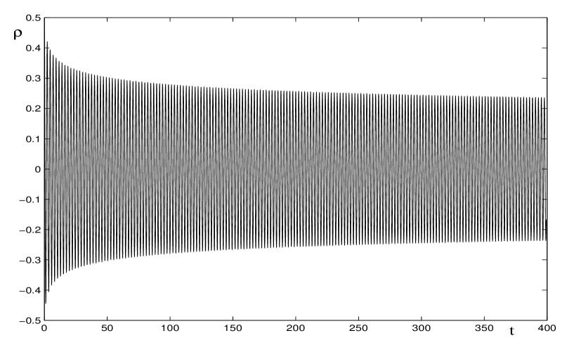
FIG. 1.: Evolution of the mean value $\rho(t)$ for $\Lambda/m_{\rm eq}=10$, $\ell=0$ and $\rho_{0}=0.5$.

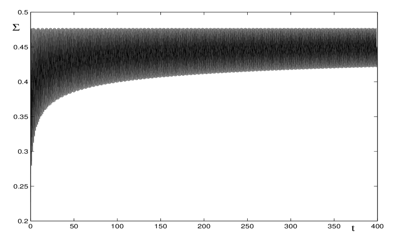
FIG. 2.: Evolution of the backreaction $\Sigma(t)$ for $\Lambda/m_{\rm eq}=10$, $\ell=0$ and $\rho_{0}=0.5$.

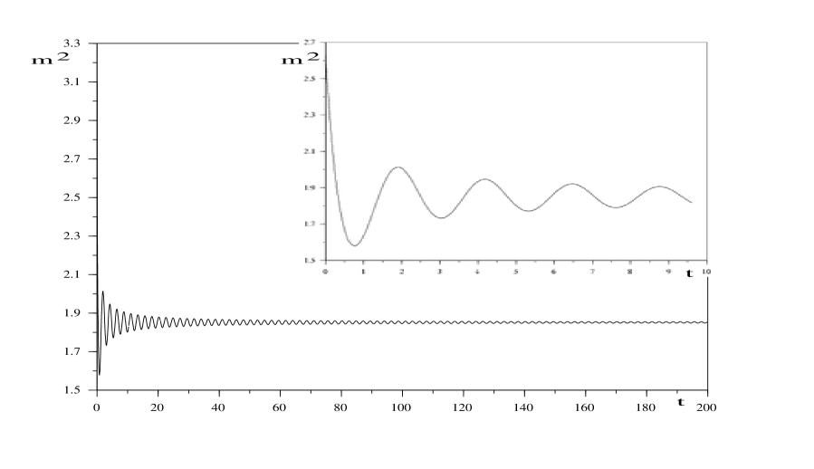
FIG. 3.: Evolution of the Lagrange multiplier $m^{2}(t)$ for $\Lambda/m_{\rm eq}=20$, $\ell=0$ and $\rho_{0}=0.3$. In the smaller figure there is zoom of the early times.

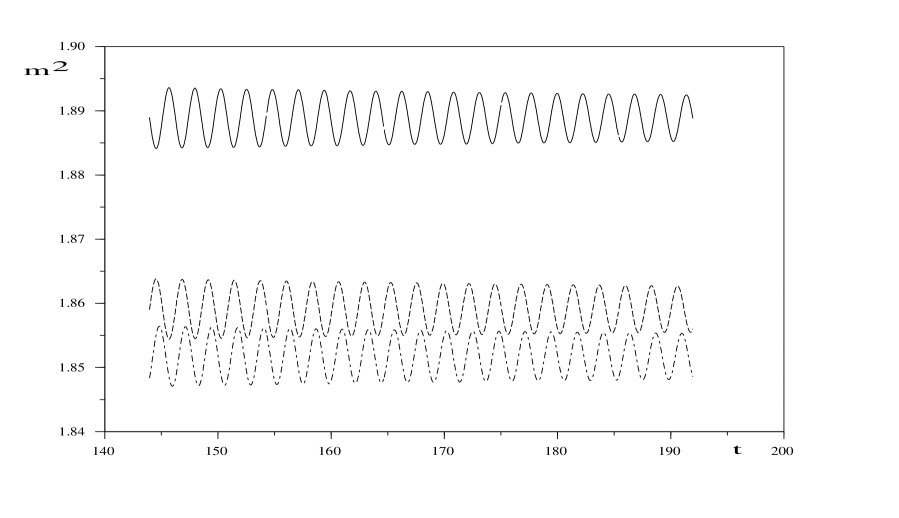
FIG. 4.: Asymptotic evolution of $m^{2}(t)$ for three different values of the ultraviolet cut–off: from top to bottom, $\Lambda/m_{\rm eq}=5,10$ and $20$, $\ell=0$ and $\rho_{0}=0.3$

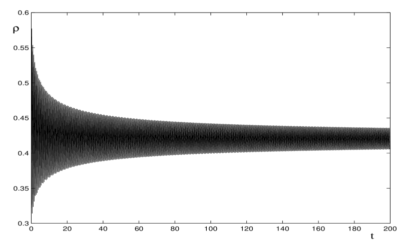
FIG. 5.: Evolution of the mean value $\rho$ for $\Lambda/m_{\rm eq}=10$, $\rho_{0}=0.3$ and $\ell=1$.

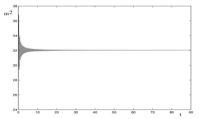
FIG. 6.: Evolution of the squared mass $m^{2}$ for $\Lambda/m_{\rm eq}=10$, $\rho_{0}=0.3$ and $\ell=1$.

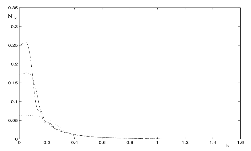
FIG. 7.: Adiabatic spectrum for $tm_{\rm eq}=0$ (solid line), $39.723$ (dotted line), $199.006$ (dashdot line) and $398.11$ (dashed line), for $\Lambda/m_{\rm eq}=20$, $\ell=0$ and $\rho_{0}=0.2$.

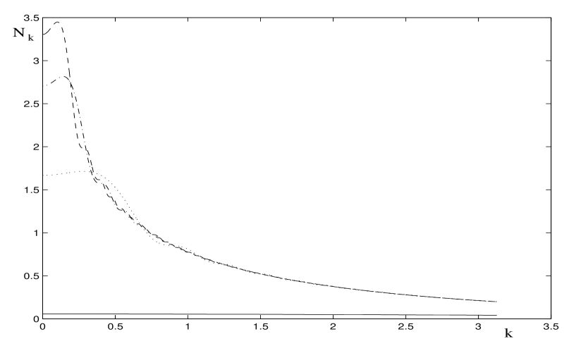
FIG. 8.: Adiabatic spectrum for $tm_{\rm eq}=0$ (solid line), $39.723$ (dotted line), $199.006$ (dashdot line) and $398.11$ (dashed line), for $\Lambda/m_{\rm eq}=20$, $\ell=0$ and $\rho_{0}=0.6$.

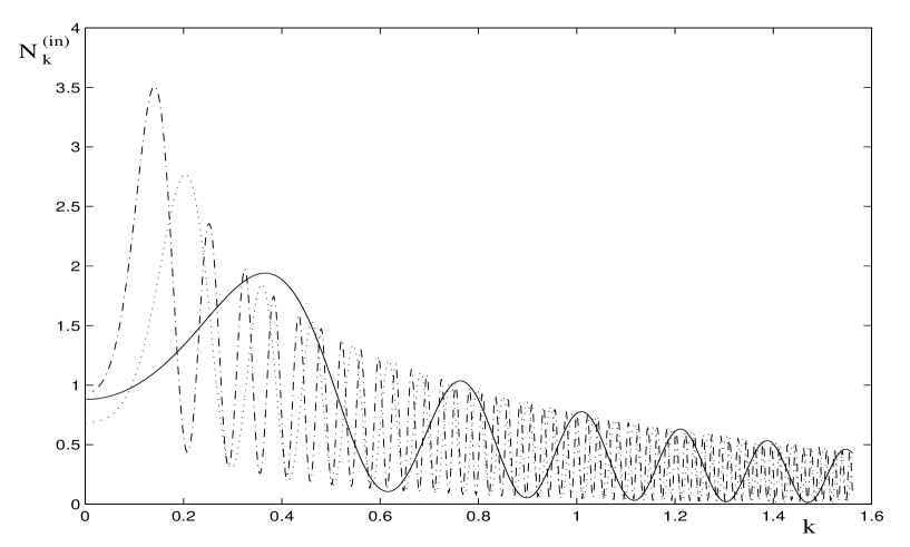
FIG. 9.: Spectrum with respect to the initial vacuum, for $tm_{\rm eq}=39.723$ (solid line), $199.006$ (dotted line) and $398.11$ (dashdot line), for $\Lambda/m_{\rm eq}=20$, $\ell=0$ and $\rho_{0}=0.5$.

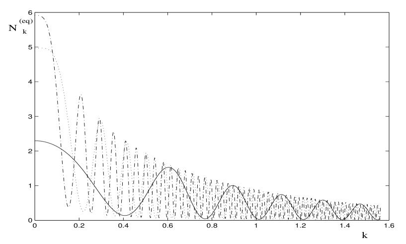
FIG. 10.: Spectrum with respect to the true vacuum, for $tm_{\rm eq}=39.723$ (solid line), $199.006$ (dotted line) and $398.11$ (dashdot line), for $\Lambda/m_{\rm eq}=20$, $\ell=0$ and $\rho_{0}=0.5$.

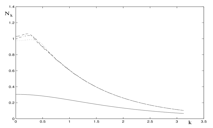
FIG. 11.: Adiabatic spectrum for $tm_{\rm eq}=0.0$ (solid line), $59.895$ (dotted line), $119.835$ (dashdot line) and $179.775$ (dashed line), for $\Lambda/m_{\rm eq}=10$, $\ell=1$ and $\rho_{0}=0.3$.

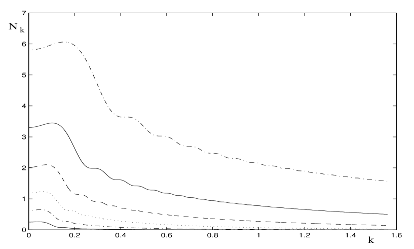
FIG. 12.: Adiabatic spectrum for $tm_{\rm eq}=398.11$, $\Lambda/m_{\rm eq}=20$ and $\ell=0$. The different curves correspond to different initial values for the condensate: from top to bottom, $\rho_{0}=0.7$, $0.6$, $0.5$, $0.4$, $0.3$ and $0.2$.

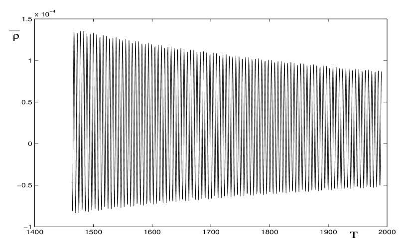
FIG. 13.: The average value of the condensate $\rho$, defined as $\bar{\rho}=\int^{T}\rho(t)dt/T$, plotted vs. $T$, for $\Lambda/m_{\rm eq}=20$, $\ell=0$ and $\rho_{0}=0.2$.

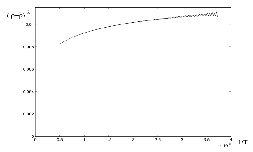
FIG. 14.: The mean squared fluctuations of the condensate $\rho$, defined as $\int^{T}(\rho(t)-\bar{\rho})^{2}dt/T$, plotted vs. $1/T$, for the same values of the parameters as in figure 13.

REFERENCES

• [1] D. Boyanovsky, H.J. de Vega and R. Holman, Phys. rev. D51 734 (1995).
• [2] D. Boyanovsky, H.J. de Vega, R. Holman, D.-S. Lee, A. Singh, Phys. Rev. D51 4419 (1995).
• [3] D. Boyanovsky, C. Destri, H.J. de Vega, R. Holman, J. Salgado, Phys.Rev. D57 7388 (1998).
• [4] F. Cooper, S. Habib, Y. Kluger, E. Mottola, Phys. Rev. D55 6471 (1997).
• [5] S. Habib, Y. Kluger, E. Mottola, J. P. Paz, Phys. Rev. Lett. 76 4660 (1996).
• [6] F. Cooper, S. Habib, Y. Kluger, E. Mottola, J.P. Paz, Phys.Rev. D50 2848 (1994).
• [7] K. G. Wilson and J. Kogut, Phys. Rep. C12 75 (1974).
• [8] J. Zinn Justin, Quantum field theory and critical phenomena (second edition), Oxford Science Publications, 1994.
• [9] M. Gell-Mann and M. Levy, Nuovo Cimento 16, 705 (1960).
• [10] B. D. Simons and A. Altland, Mesoscopic Physics, lectures given to the β€œIXth CRM Summer School, 1999: Theoretical Physics at the End of the XXth Century”, Banff, Alberta, Canada, June 27 - July 10, 1999.
• [11] L. G. Yaffe, Rev of Mod. Phys. 54 407 (1982).
• [12] L.-H. Chan, Phys. Rev. D36 3755 (1987).
• [13] C. Destri, E. Manfredini, Out–of–equilibrium dynamics of large$-N$ $\phi^{4}$ QFT in finite volume, IFUM 650/FT-99, Bicocca-FT-99-37, hep-ph/0001177. Accepted for publication in Physical Review D.
• [14] N. D. Mermin, H. Wagner, Phys. Rev. Lett. 17 1133 (1966); S. Coleman, Commun. Math Phys. 31 259 (1973).
• [15] D. Boyanovsky, H.J. de Vega, R. Holman, Phys. Rev. D49 2769 (1994).
• [16] C. Destri, E. Manfredini, work in progress.