Self-Breaking of the Standard Model
Gauge Symmetry

If the gauge fields of the Standard Model propagate in TeV-size extra dimensions, they rapidly become strongly coupled and can form scalar bound states of quarks and leptons. If the quarks and leptons of the third generation propagate in 6 or 8 dimensions, we argue that the most tightly bound scalar is a composite of top quarks, having the quantum numbers of the Higgs doublet and a large coupling to the top quark. In the case where the gauge bosons propagate in a bulk of a certain volume, this composite Higgs doublet can successfully trigger electroweak symmetry breaking. The mass of the top quark is correctly predicted to within 20%, without the need to add a fundamental Yukawa interaction, and the Higgs boson mass is predicted to lie in the range 165 - 230 GeV. In addition to the Higgs boson, there may be a few other scalar composites sufficiently light to be observed at upcoming collider experiments.

1 Introduction and Conclusions

The Standard Model (SM) has three main ingredients: 1) the $SU(3)_{C}\times SU(2)_{W}\times U(1)_{Y}$ gauge group; 2) three generations of quarks and leptons; 3) a Higgs doublet. As opposed to the gauge group and fermion representations which may be viewed as natural low-energy remnants of an unified theory, the Higgs doublet is an ad hoc addition required solely to break the electroweak symmetry and to accommodate the observed fermion masses. In this paper we show that the existence of a Higgs doublet is a consequence of ingredients 1) and 2) provided the gauge bosons and fermions propagate in appropriate extra dimensions compactified at a scale in the TeV range.

Given that gauge theories are non-renormalizable in more than four dimensions, there is need for a physical cutoff, $M_{s}$, above but not far from the compactification scale. An obvious candidate for this cutoff is the scale of quantum gravity, as would occur if the gravitational coupling becomes strong at a scale in the TeV range. This may be achieved if the space accessible to Standard Model fields is embedded in a large volume accessible only to the gravitons [1], or if there are warped extra dimensions [2]. An alternative possibility is that the theory becomes embedded in some other consistent ultraviolet completion of higher-dimensional gauge theory without gravity, while the scale of quantum gravity is higher.

Below the cutoff scale $M_{s}$, we are dealing with an effective field theory which includes the $SU(3)_{C}\times SU(2)_{W}\times U(1)_{Y}$ gauge group and three generations of fermions in compact dimensions. The basic idea is that the higher-dimensional gauge interactions become strong at the scale $M_{s}$ and produce fermion–anti-fermion bound states. It is very significant that, with plausible dynamical assumptions, the charges of the quarks and the leptons under the Standard Model gauge group are such that the most deeply bound state which transforms non-trivially under the gauge group is a Higgs doublet. Thus, a composite Higgs doublet which acquires an electroweak asymmetric vacuum expectation value could result as a direct consequence of the extra dimensions.

Previously, it has been shown that the combined effect of the Kaluza-Klein (KK) modes of the gluons is strong enough [3] to give rise to a composite Higgs doublet made of the four-dimensional left-handed top-bottom doublet and a five-dimensional top-quark field [4]. More generally, the strong dynamics intrinsically associated with gauge interactions in extra dimensions is a good candidate for viable theories without a fundamental Higgs doublet [5].

Here we consider the more natural setup where a full generation (the “third” one by definition) propagates in extra dimensions of TeV^-1 size, and the higher-dimensional $SU(3)_{C}\times SU(2)_{W}\times U(1)_{Y}$ interactions induce electroweak symmetry breaking. In section 2 we study the possible bound states and symmetry breaking pattern of the higher-dimensional gauge dynamics using the most attractive channel (MAC) analysis. A more detailed description of the bound states using the Nambu–Jona-Lasinio (NJL) approximation is presented in section 3. Remarkably enough, it turns out that the composite Higgs doublet has a Yukawa coupling of order one only to the top quark. The model includes potentially light composite scalars other than the Higgs boson, which could be within the reach of future collider experiments.

Despite the uncertainties due to the cutoff scale, we are able to obtain rather reliable predictions for the top and Higgs masses because the renormalization group (RG) equations exhibit infrared fixed points. The top mass is predicted with a ${\cal O}(20\%)$ uncertainty, and is consistent with the experimental value. The Higgs boson mass is predicted in the $165-230$ GeV range (section 4).

More generally, extra dimensions accessible to Standard Model fields provide a natural setting for theories with composite Higgs fields. Normally, in four dimensions, these theories suffer from the difficulty that the SM Yukawa couplings look quite perturbative; even for the top quark $\lambda_{t}\sim 1$ rather than $\sim 4\pi$. On the other hand, in any theory with a composite Higgs, the Yukawa couplings are expected to blow up at the compositeness scale. This either predicts too large a top quark mass if this scale is low, or requires us to push the compositeness scale up so high that the usual hierarchy problem fine-tune is needed to keep the Higgs light [6, 7]. Theories with extra dimensions allow for a way out of this problem: all the fundamental higher-dimensional couplings, including the gauge and Yukawa couplings, can be strong, while the effective four-dimensional couplings can be perturbative due to a moderate dilution factor from the volume of the extra dimensions. More precisely, strong dynamics can trigger a composite Higgs to form in higher dimensions with the associated large couplings, but the power-law running of couplings in higher dimensions allow these couplings to reach perturbative infrared fixed points without the need to push the compositeness scale to grand unification scale values. The discussion of section 4 for the top and Higgs masses holds in any such higher-dimensional theory, with the “composite” boundary conditions that the top Yukawa and Higgs quartic couplings blow up at the ultraviolet cutoff.

In section 5 we mention various scenarios with three generations in which some flavor non-universal effects prevent the up and charm quarks from forming deeply bound states at the scale $M_{s}$, while also allowing the light quarks and leptons to obtain their masses. Finally, we conclude with a comparison between our scenario and the supersymmetric extensions of the Standard Model in section 6.

2 A Third Generation Model

Let us consider the Standard Model gauge group and one generation (the “third” one) of fermions in $D$ dimensions, where four of them are the usual Minkowski spacetime and $D-4$ spatial dimensions are compactified at a scale $1/R$ of a few TeV. For even $D$, there is an analogue of the four-dimensional $\gamma_{5}$ matrix, $\Gamma_{D+1}$, hence chiral fermions with eigenvalues $\pm 1$ of $\Gamma_{D+1}$ exist. Nonetheless, the higher-dimensional fermions have four or more components. In order to obtain a four-dimensional chiral theory, the extra dimensions must be compactified on an orbifold or with some boundary conditions such that the zero modes of one four-dimensional chirality are projected out. We will concentrate mostly on the case of chiral fermions in even number of extra dimensions, leaving the more complicated discussion of vector-like fermions in $D\geq 5$ for the Appendix.

We assign $SU(2)_{W}$ doublets with positive chirality, ${\cal Q}_{+}$, ${\cal L}_{+}$, and $SU(2)_{W}$ singlets with negative chirality, ${\cal U}_{-}$, ${\cal D}_{-}$, ${\cal E}_{-}$. Each fermion contains both left- and right-handed two-component spinors when reduced to four dimensions. We impose an orbifold projection such that the right-handed components of ${\cal Q}_{+}$, ${\cal L}_{+}$, and left-handed components of ${\cal U}_{-}$, ${\cal D}_{-}$, ${\cal E}_{-}$, are odd under the orbifold ${\bf Z}_{2}$ symmetry and therefore the corresponding zero modes are projected out. As a result, the zero-mode fermions are two-component four-dimensional quarks and leptons: ${\cal Q}_{+}^{(0)}\equiv(t,b)_{L}$,   ${\cal U}_{-}^{(0)}\equiv t_{R}$,   ${\cal D}_{-}^{(0)}\equiv b_{R}$,   ${\cal L}_{+}^{(0)}\equiv(\nu_{\tau},\tau)_{L}$, ${\cal E}_{-}^{(0)}\equiv\tau_{R}$.

Given that the massless fermion spectrum (before electroweak symmetry breaking) is a full generation of Standard Model fermions, the theory is obviously free from four-dimensional anomalies. Nevertheless, there may be $D$-dimensional anomalies because the theory is chiral. There are no $SU(3)_{C}$ anomalies because the fermions have vector-like strong interactions. Similarly, the unbroken $U(1)_{EM}$ is anomaly free, and the gravitational anomaly cancels if we include a singlet with negative chirality. (Its zero-mode can be identified as a right-handed neutrino.) On the other hand, the $SU(2)_{W}$ and $U(1)_{Y}$ representations are chiral and there are $[SU(2)_{W}]^{D/2+1}$, $[U(1)_{Y}]^{D/2+1}$ and mixed anomalies. These $D$-dimensional anomalies, however, can be canceled by the Green-Schwarz mechanism [8]. We will assume the presence of such a Green-Schwarz counterterm in the effective Lagrangian so that the full theory is non-anomalous. This term will not play any role in the following discussion.

At the cutoff scale, $M_{s}$, the Standard Model gauge interactions are non-perturbative and produce bound states. Some of the scalar bound states may have squared-masses significantly smaller than $M_{s}^{2}$, due to the quadratic dependence on the cutoff of their self-energies [9]. We do not expect that the interactions which are strong in the ultraviolet exhibit confinement, because at large distance ($R<r<\Lambda_{\rm QCD}^{-1}$) only the zero modes of the gauge fields are relevant and the interactions are not strong. The effective theory below $M_{s}$ involves both fermions and composite scalars. The squared-mass of the composite scalar decreases when the strength of the attractive interaction that produces the bound state increases. For a sufficiently strong attractive interaction, the squared-mass turns negative inducing chiral symmetry breaking.

In order to study the low-energy theory and the symmetry breaking pattern, we need to identify the most attractive scalar channels [10]. In the one-gauge-boson-exchange approximation, the binding strength of a $\overline{\psi}\chi$ channel is proportional to

$$\hat{g}_{3}^{2}{\bf T}_{\overline{\psi}}\cdot{\bf T}_{\chi}+\hat{g}_{2}^{2}{\bf T^{\prime}}_{\overline{\psi}}\cdot{\bf T^{\prime}}_{\chi}+\hat{g}^{\prime 2}Y_{\psi}Y_{\chi}$$ (2.1)

where $\hat{g}_{3}$, $\hat{g}_{2}$ and $\hat{g}^{\prime}$ are the six-dimensional $SU(3)_{C}\times SU(2)_{W}\times U(1)_{Y}$ gauge couplings at the cutoff scale, ${\bf T}$ and ${\bf T^{\prime}}$ are the $SU(3)_{C}\times SU(2)_{W}$ generators of the corresponding fermion, and $Y$ is the hypercharge. For computing the relative strength of various channels it is convenient to use the following identity:

$${\bf T}_{\overline{\psi}}\cdot{\bf T}_{\chi}=\frac{1}{2}\left[C_{2}\left(\overline{\psi}\right)+C_{2}\left(\chi\right)-C_{2}\left(\overline{\psi}\chi\right)\right]~{},$$ (2.2)

where $C_{2}(r)$ is the second Casimir invariant for the representation $r$ of the gauge group.

The bound states which can be formed depend on the transformation of the higher-dimensional fermions under charge conjugation. Therefore, we will consider separately the cases of $D=4k+2$ and $D=4k+4$ with $k\geq 1$ integer.

2.1 Fermions in six dimensions ($D=4k+2$)

We first study a six-dimensional [or more generally, $(4k+2)$-dimensional] theory with chiral fermions. Note that these are dimensions larger than $M_{s}^{-1}$ accessible to the quarks and leptons, and the discussion that follows does not depend on the existence of other dimensions which are either smaller than $M_{s}^{-1}$ or inaccessible to the Standard Model fields.

In ($4k+2$) dimensions, the charge conjugation does not change the chirality, in contrast with the $4k$-dimension cases. Therefore, ${{\cal Q}}^{c}_{+}$, ${{\cal L}}^{c}_{+}$ still have positive chirality and ${{\cal U}}^{c}_{-}$, ${{\cal D}}^{c}_{-}$, ${{\cal E}}^{c}_{-}$ have negative chirality. The light bound states are $(4k+2)$-dimensional scalars, and their constituents have the $\overline{\psi}_{+}\chi_{-}$ form.

In Table 1 we list all the attractive scalar channels and the binding strength of the composite scalars in the MAC approximation. The higher-dimensional gauge couplings $\hat{g}_{i}$ are related to the four-dimensional ones by the volume of the $D-4$ compact dimensions, $\hat{g}_{i}=g_{i}\sqrt{V_{D-4}}$. We use the $SU(5)$ normalization for the hypercharge gauge coupling, where $\hat{g}^{\prime 2}=(3/5)\hat{g}_{1}^{2}$. We denote the scalars transforming as the left-handed doublet quark under the SM gauge group by $\tilde{q}$, borrowing the notation from supersymmetry, and the scalars transforming as $({\bf 3,2},-5/6)$ under SM gauge group by $X$.

Composite scalar	constituents	$SU(3)\times SU(2)\times U(1)$ representation	binding strength	relative binding for $\hat{g}_{1}=\hat{g}_{2}=\hat{g}_{3}$
$H_{\cal U}$	$\overline{\cal Q}_{+}{\cal U}_{-}$	$({\bf 1,2,}+1/2)$	$\frac{4}{3}\hat{g}_{3}^{2}+\frac{1}{15}\hat{g}_{1}^{2}$	1
$H_{\cal D}$	$\overline{\cal Q}_{+}{\cal D}_{-}$	$({\bf 1,2,}-1/2)$	$\frac{4}{3}\hat{g}_{3}^{2}-\frac{1}{30}\hat{g}_{1}^{2}$	$0.93$
$\tilde{q}$	$\overline{\cal Q}_{+}{\cal D}^{c}_{-}$	$({\bf{3},2,}+1/6)$	$\frac{2}{3}\hat{g}_{3}^{2}+\frac{1}{30}\hat{g}_{1}^{2}$	$0.5$
$X$	$\overline{\cal Q}_{+}{\cal U}^{c}_{-}$	$({\bf{3},2,}-5/6)$	$\frac{2}{3}\hat{g}_{3}^{2}-\frac{1}{15}\hat{g}_{1}^{2}$	$0.43$
$H_{\cal E}$	$\overline{\cal L}_{+}{\cal E}_{-}$	$({\bf 1,2,}-1/2)$	$\frac{3}{10}\hat{g}_{1}^{2}$	$0.21$
$\tilde{q}^{\prime}$	$\overline{\cal L}^{c}_{+}{\cal U}_{-}$	$({\bf{3},2,}+1/6)$	$\frac{1}{5}\hat{g}_{1}^{2}$	$0.14$
$\tilde{q}^{\prime\prime}$	$\overline{\cal L}_{+}{\cal D}_{-}$	$({\bf 3,2,}+1/6)$	$\frac{1}{10}\hat{g}_{1}^{2}$	$0.07$
$X^{\prime}$	$\overline{\cal Q}^{c}_{+}{\cal E}_{-}$	$({\bf{3},2,}-5/6)$	$\frac{1}{10}\hat{g}_{1}^{2}$	$0.07$

Table 1: Attractive scalar channels in six dimensions with chiral fermions

Although composite operators such as $\overline{{\cal Q}}_{+}\Gamma_{\alpha}{\cal Q}_{+}$, where $\alpha=5,...,D$, are also scalars in four dimensions, (reduced to $\overline{q}_{L}q_{R}\pm\overline{q}_{R}q_{L}$ in the two-component spinor notation,) they belong to the vector channels in $D$ dimensions. We make the usual dynamical assumption that Lorentz invariance is not spontaneously broken by the strong gauge dynamics. If these vector bound states do form, we assume that their masses are close to the cutoff scale. Although the $D$-dimensional Lorentz invariance is broken by the compactification, this breaking occurs at a scale significantly lower than the cutoff scale where the interactions become strong and the bound states are formed, so it should have little effect.

Above the compactification scale, the running of the four-dimensional gauge couplings becomes power-law [11] due to the presence of the KK modes. The convergence of the three SM gauge couplings is accelerated. One typically finds that at the scale where the gauge interactions become non-perturbative, the three gauge couplings become comparable and are consistent with unification within theoretical uncertainties [12]. Since the binding force is dominated by ultraviolet interactions, the $SU(2)_{W}$ and $U(1)_{Y}$ interactions could be as important as the $SU(3)_{C}$ interaction. In Table 1 we also list the relative binding strength for all the attractive scalar channels by assuming $\hat{g}_{1}=\hat{g}_{2}=\hat{g}_{3}$. In order to avoid proton decay we do not invoke a unified gauge group, and simply assume that physics above $M_{s}$ preserves baryon number. However, if there was a unified gauge group at $M_{s}$, then the exchange of the additional gauge bosons would modify the binding strength.

An inspection of Table 1 shows that the most deeply bound states are the six-dimensional $H_{\cal U}$ and $H_{\cal D}$ scalars, which transform under the gauge group as the Standard Model Higgs doublet. Note that this is true for a wide range of couplings $\hat{g}_{i}$; gauge coupling unification is not a necessity. These scalars have large Yukawa couplings to their constituents, $\overline{\cal Q}_{+}{\cal U}_{-}$ and $\overline{\cal Q}_{+}{\cal D}_{-}$ respectively. $H_{\cal U}$ is more strongly bound than $H_{\cal D}$, so that it naturally acquires a vacuum expectation value (VEV), breaking $SU(2)_{W}\times U(1)_{Y}$ down to $U(1)_{EM}$. Furthermore, if the binding strength of $H_{\cal U}$ is not much larger than the critical value where the squared-mass of $H_{\cal U}$ turns negative, then the VEV of $H_{\cal U}$ will be below the compactification scale. Hence, the zero mode of $H_{\cal U}$ plays the role of the SM Higgs doublet.

In the one-gauge boson exchange approximation, the squared-mass of $H_{\cal D}$ is expected to stay positive, because of the difference in the hypercharge interaction which also becomes strong, though significantly smaller than the compositeness scale. The other composite scalars, $H_{\cal E}$, $\tilde{q}$, $\tilde{q}^{\prime}$, $\tilde{q}^{\prime\prime}$, $X$, and $X^{\prime}$ are not likely to be sufficiently strongly bound for being relevant at low energies. Therefore, we have a compelling picture, in which the electroweak symmetry is correctly broken and only the top quark acquires a large mass. The low-energy effective theory below $1/R$ is simply the Standard Model plus a possible additional Higgs doublet (the zero mode of $H_{\cal D}$).

2.2 Fermions in eight dimensions ($D=4k+4$)

In eight dimensions (or more generally in $D=4k+4$ with $k\geq 1$) with chiral fermions, there are some different bound states because charge conjugation flips the chirality. Besides $H_{\cal U}$, $H_{\cal D}$, $H_{\cal E}$, and $\tilde{q}^{\prime\prime}$, there are four more bound states transforming like the right-handed down-type quark under the SM gauge transformation (see Table 2). Among them, the bound state $\tilde{b}=\overline{{\cal Q}}_{+}{\cal Q}^{c}_{-}$ is also strongly bound and in the MAC approximation would have the same binding strength as $H_{\cal U}$ if all three SM gauge couplings had the same strength. The degeneracy is accidental and will not be exact. For example, by taking into account the effect of running couplings, the $\overline{{\cal Q}}_{+}{\cal Q}^{c}_{-}$ channel will be somewhat weaker than the Higgs channel $\overline{{\cal Q}}_{+}{\cal U}_{-}$ even if we assume $\hat{g}_{3}=\hat{g}_{2}=\hat{g}_{1}$ at the cutoff scale, because the contributions coming from scales below $M_{s}$ have $\hat{g}_{2}<\hat{g}_{3}$. Nevertheless, the composite scalar $\tilde{b}$ is expected to be quite light if the squared-mass of $H_{\cal U}$ becomes negative. The VEV of $H_{\cal U}$ will give a positive contribution to the squared-mass of $\tilde{b}$, and hence prevents $\tilde{b}$ from acquiring a nonzero VEV and breaking the color gauge group. The low-energy theory in this case is a two-Higgs-doublet model plus a charged color triplet scalar.

Composite scalar	constituents	$SU(3)\times SU(2)\times U(1)$ representation	binding strength	relative binding for $\hat{g}_{1}=\hat{g}_{2}=\hat{g}_{3}$
$H_{\cal U}$	$\overline{\cal Q}_{+}{\cal U}_{-}$	$({\bf 1,2,}+1/2)$	$\frac{4}{3}\hat{g}_{3}^{2}+\frac{1}{15}\hat{g}_{1}^{2}$	1
$H_{\cal D}$	$\overline{\cal Q}_{+}{\cal D}_{-}$	$({\bf 1,2,}-1/2)$	$\frac{4}{3}\hat{g}_{3}^{2}-\frac{1}{30}\hat{g}_{1}^{2}$	$0.93$
$\tilde{b}$	$\overline{\cal Q}_{+}{\cal Q}^{c}_{-}$	$({\bf 3,1,}-1/3)$	$\frac{2}{3}\hat{g}_{3}^{2}+\frac{3}{4}\hat{g}_{2}^{2}-\frac{1}{60}\hat{g}_{1}^{2}$	$1-\epsilon$
$\tilde{b}^{\prime}$	$\overline{\cal U}_{-}{\cal D}^{c}_{+}$	$({\bf 3,1,}-1/3)$	$\frac{2}{3}\hat{g}_{3}^{2}+\frac{2}{15}\hat{g}_{1}^{2}$	$0.57$
$\tilde{b}^{\prime\prime}$	$\overline{\cal Q}^{c}_{-}{\cal L}_{+}$	$({\bf{3},1,}-1/3)$	$\frac{3}{4}\hat{g}_{2}^{2}+\frac{1}{20}\hat{g}_{1}^{2}$	$0.57$
$\tilde{b}^{\prime\prime\prime}$	$\overline{\cal U}^{c}_{+}{\cal E}_{-}$	$({\bf{3},1,}-1/3)$	$\frac{2}{5}\hat{g}_{1}^{2}$	$0.29$
$H_{\cal E}$	$\overline{\cal L}_{+}{\cal E}_{-}$	$({\bf 1,2,}-1/2)$	$\frac{3}{10}\hat{g}_{1}^{2}$	$0.21$
$\tilde{q}^{\prime\prime}$	$\overline{\cal L}_{+}{\cal D}_{-}$	$({\bf 3,2,}+1/6)$	$\frac{1}{10}\hat{g}_{1}^{2}$	$0.07$

Table 2: Attractive scalar channels in eight dimensions with chiral fermions. We include an $\epsilon>0$ in the $\tilde{b}$ channel to account for the lifting of the degeneracy due to the running coupling effect below $M_{s}$.

3 Four-fermion Operator Approximation

In the previous section we have studied the formation of bound states using a most attractive channel approximation. A more detailed study of the bound state properties may be based on the following considerations.

The higher-dimensional gauge interactions become strong at the ultraviolet cutoff, and therefore the high-momentum gauge fields give the dominant interaction between the fermions. The picture described in the previous section can be studied in a more quantitative manner by approximating the dynamics of the higher-dimensional gauge interactions with an effective theory involving four-fermion operators suppressed by a scale $\Lambda\sim M_{s}$:

$$\int d^{D}\!x\frac{-1}{2\Lambda^{2}} \left[\hat{g}_{3}^{2}\left(\overline{\cal Q}_{+}\Gamma^{\alpha}T^{r}{\cal Q}_{+}+\overline{\cal U}_{-}\Gamma^{\alpha}T^{r}{\cal U}_{-}\!\!+\overline{\cal D}_{-}\Gamma^{\alpha}T^{r}{\cal D}_{-}\right)^{2}+\hat{g}_{2}^{2}\bigg{(}\overline{\cal Q}_{+}\Gamma^{\alpha}\frac{\textstyle\vec{\sigma}}{\textstyle 2}{\cal Q}_{+}+\overline{\cal L}_{+}\Gamma^{\alpha}\frac{\textstyle\vec{\sigma}}{\textstyle 2}{\cal L}_{+}\bigg{)}^{2}\right.$$ (3.1)

$$\left.+\frac{\textstyle 3}{\textstyle 5}\hat{g}_{1}^{2}\bigg{(}\frac{\textstyle 1}{\textstyle 6}\overline{\cal Q}_{+}\Gamma^{\alpha}{\cal Q}_{+}+\frac{\textstyle 2}{\textstyle 3}\overline{\cal U}_{-}\Gamma^{\alpha}{\cal U}_{-}-\frac{\textstyle 1}{\textstyle 3}\overline{\cal D}_{-}\Gamma^{\alpha}{\cal D}_{-}-\frac{\textstyle 1}{\textstyle 2}\overline{\cal L}_{+}\Gamma^{\alpha}{\cal L}_{+}-\overline{\cal E}_{-}\Gamma^{\alpha}{\cal E}_{-}\bigg{)}^{2}\,\right]~{},\!\!$$

where $\sigma$ are the Pauli matrices.

To be concrete, we study the $D=6$ case in this section. The fermion fields depend on the spacetime coordinates $x^{\alpha}$, labeled by $\alpha=0,1,2,3,5,6$, where $x^{5}$ and $x^{6}$ are compact, of size $\pi R$. The six-dimensional gamma matrices are given in terms of the four-dimensional ones by, e.g.,

$$\Gamma^{\mu}=\left(\begin{array}[]{cc}-\gamma^{\mu}&0\\ 0&\gamma^{\mu}\end{array}\right)\;,\;\mu=0,1,2,3,\;\;\;\Gamma^{5}=\left(\begin{array}[]{cc}0&i{\bf I}\\ i{\bf I}&0\end{array}\right)\;\;,\;\;\;\Gamma^{6}=\left(\begin{array}[]{cc}0&{\bf I}\\ -{\bf I}&0\end{array}\right)\;~{},$$ (3.2)

and the 6-dimensional chiral projection operators are defined by

$$P_{\pm}\equiv\frac{1\pm\Gamma_{7}}{2}=\frac{1}{2}\left(\begin{array}[]{cc}1\mp\gamma_{5}&0\\ 0&1\pm\gamma_{5}\end{array}\right)~{}.$$ (3.3)

The four-fermion operators (3.1) may be analyzed along the lines presented in [4]. The scalar channel operators can be obtained after Fierz transformation,

$$\int d^{6}x\frac{3}{2\Lambda^{2}}\left[c_{\cal U}\left(\overline{\cal Q}_{+}{\cal U}_{-}\right)\left(\overline{\cal U}_{-}{\cal Q}_{+}\right)+c_{\cal D}\left(\overline{\cal Q}_{+}{\cal D}_{-}\right)\left(\overline{\cal D}_{-}{\cal Q}_{+}\right)\right]+\cdots,$$ (3.4)

where $c_{\cal U}$, $c_{\cal D}$ are the binding strength for the corresponding channels, which in the simplest approximation are proportional to the value obtained in the MAC analysis, ($\frac{4}{3}\hat{g}_{3}^{2}+\frac{1}{15}\hat{g}_{1}^{2},\,\frac{4}{3}\hat{g}_{3}^{2}-\frac{1}{30}\hat{g}_{1}^{2}$,) and the ellipsis stand for vectorial and tensorial four-fermion operators, which are irrelevant at low energies, as well as four-fermion operators in the scalar channels that do not produce light scalars.

The operators shown above give rise to composite scalars whose kinetic terms vanish at a scale $\sim M_{s}$. Therefore, these scalars are physical degrees of freedom only below $M_{s}$. We derive the low-energy effective Lagrangian following the steps described in [4]. First, the scalar self-energies and quartic couplings are induced by the interactions with their constituents. These may be computed in the large-$N_{c}$ limit, where only one fermion loop contributes. Then the scalar fields may be redefined to allow canonical normalization of their kinetic terms. This yields a six-dimensional effective action which includes the following terms involving scalars:

$$-\int d^{6}x\left[V_{6}+\frac{\xi}{M_{s}}\left(\overline{\cal U}_{-}{\cal Q}_{+}H_{\cal U}+\overline{\cal D}_{-}{\cal Q}_{+}H_{\cal D}+{\rm h.c.}\right)\right]~{},$$ (3.5)

where the effective potential is given by

$$V_{6}=\frac{\lambda}{2M_{s}^{2}}\left(H_{\cal U}^{\dagger}H_{\cal U}+H_{\cal D}^{\dagger}H_{\cal D}\right)^{2}+M_{H_{\cal U}}^{2}H_{\cal U}^{\dagger}H_{\cal U}+M_{H_{\cal D}}^{2}H_{\cal D}^{\dagger}H_{\cal D}~{}.$$ (3.6)

The quartic and Yukawa couplings satisfy the usual NJL relation for large-$N_{c}$,

$$\lambda=2\xi^{2}~{}.$$ (3.7)

The scalar squared-masses are strongly dependent on the cutoff, but this does not affect the features important for the low-energy theory, namely their sign and relative sizes:

$$\left(M^{2}_{H_{\cal U}},\ M^{2}_{H_{\cal D}}\right)\approx\frac{16\pi^{2}F}{3N_{c}}\left(\frac{1}{c_{\cal U}},\,\frac{1}{c_{\cal D}}\right)-F^{\prime}\Lambda^{2}~{},$$ (3.8)

where the first term is the bare mass re-scaled by the wave function renormalization and the second term comes from the fermion loop. $F$ and $F^{\prime}$ are positive coefficients of order one that may be computed as in [4], by summing the loop integrals corresponding to different KK modes. The binding strength $c_{\cal U},\,c_{\cal D}$ are proportional to the square of the six-dimensional gauge couplings and have dimensions of mass^-2 and are large in $M_{s}$ units, resulting in $M^{2}_{H_{\cal U}}<0$.

The minimum of $V_{6}$ is manifestly at $\langle H_{\cal U}\rangle\neq 0$ and $\langle H_{\cal D}\rangle=0$. Given that the compactification scale is above the electroweak scale, the binding strength needs to be adjusted close to the critical value where $M^{2}_{H_{\cal U}}$ becomes negative. The binding strength depends on the strength of the higher-dimensional gauge couplings; holding the effective four-dimensional gauge couplings fixed, this can be adjusted by changing the volume of the extra dimensions. The tuning that needs to be done to keep the Higgs light is not severe, since $M_{s}$ is less than a factor of five higher than $1/R$ [12].

At scales below $1/R$ the two extra dimensions are integrated out, and the four-dimensional effective theory is given by the Standard Model, (we describe the inclusion of three generations in section 5,) with the addition of a second Higgs doublet (the $H_{\cal D}$ zero-mode).

In terms of the four-dimensional KK modes, the SM Higgs $H_{U}\equiv H_{\cal U}^{(0)}$ is a bound state of all the KK modes of ${\cal U}_{-}$ and ${\cal Q}_{+}$:

$$H_{U}\sim\sum_{k=0}^{N_{\rm KK}-1}\overline{\cal Q}_{+}^{(k)}{\cal U}_{-}^{(k)}~{}.$$ (3.9)

The coupling of $H_{U}$ to each ${\cal Q}_{+}^{(k)}$ and ${\cal U}_{-}^{(k)}$ mode is suppressed by $\sqrt{N_{\rm KK}}$ compared with a four-dimensional top condensate model. Therefore, the top quark mass is also suppressed by $\sqrt{N_{\rm KK}}$ compared with the $\sim 600$ GeV value expected in the minimal four-dimensional top condensate model [7] with a TeV cutoff scale.

In the leading $N_{c}$ approximation, the NJL relation (3.7) is preserved after dimensional reduction. This implies that the Higgs boson mass, $M_{h}$, is also suppressed by $\sqrt{N_{\rm KK}}$ and is given by $2m_{t}\approx 350$ GeV in the large $N_{c}$ limit. This suppression can also be understood as the volume factor of the compact dimensions, ($N_{\rm KK}=V_{D-4}M_{s}^{D-4}$.) Because the Higgs doublet and the fermions live in extra dimensions, the four-dimensional top Yukawa coupling and Higgs self-coupling are related to the higher-dimensional ones by the volume factor:

$$\lambda_{t}=\frac{\xi}{\sqrt{V_{D-4}M_{s}^{D-4}}}\;\;,\;\;\lambda_{h}=\frac{\lambda}{V_{D-4}M_{s}^{D-4}}~{}.$$ (3.10)

By contrast, in top-quark seesaw models [13], as well as in the model with only $t_{R}$ in extra dimensions [4], the Higgs boson is heavy, at the triviality bound, unless there is large mixing among scalars.

The above discussion only includes the leading $N_{c}$ contribution, i.e. fermion loops. To get a more precise prediction of the top and Higgs masses, one should also include the loop contributions from gauge bosons and scalars. This can be done by computing the full one-loop RG equations, and evolving the couplings from $M_{s}$ down to the electroweak scale. The running of the quartic Higgs coupling further decreases the physical Higgs boson mass. We study this effect in the next section.

4 Top and Higgs Mass Predictions

The more precise predictions of the top quark mass and Higgs mass can be obtained from running the corresponding (four-dimensional) couplings from the compositeness scale $M_{s}$, with the compositeness boundary condition, $\lambda_{t},\,\lambda_{h}\to\infty$ at $M_{s}$ [7], down to low energies. The running is accelerated by the power-law between the compositeness scale $M_{s}$ and the compactification scale $M_{c}=1/R$, so the effect is significant even though the two scales are not far apart. The low-energy predictions are governed by the infrared fixed points of the RG equations [15]. The infrared fixed points are determined by the $\beta$-function coefficients coming from the KK modes, which are different from those in the four-dimensional Standard Model.

The one-loop RG equations for the (four-dimensional) SM gauge couplings above $M_{c}$ are given by

$$16\pi^{2}\frac{dg_{i}}{d\ln\mu}=N_{\rm KK}(\mu)\,b^{\prime}_{i}g_{i}^{3},$$ (4.1)

where $N_{\rm KK}(\mu)$ is the number of KK modes below the scale $\mu$, [$N_{\rm KK}(\mu)=X_{\delta}(\mu R)^{\delta},\,X_{\delta}=\pi^{\delta/2}/\Gamma(1+\delta/2)$ in the continuous limit,] and $b^{\prime}_{i}$ are

$$b^{\prime}_{3} = -11+\frac{2}{3}\,m\,n_{g}+\frac{1}{2}\delta+\Delta_{3},$$

$$b^{\prime}_{2} = -\frac{22}{3}+\frac{2}{3}\,m\,n_{g}+\frac{1}{3}\delta+\frac{1}{6}n_{H}+\Delta_{2},$$

$$b^{\prime}_{1} = \frac{2}{3}\,m\,n_{g}+\frac{1}{10}n_{H}+\Delta_{1},$$ (4.2)

$m$ is the number of fermion components, ($m=4,\,8$ for 6- and 8-dimensional chiral theories respectively,) $n_{g}$ is the number of generations in the bulk (assumed to be 1 throughout most of this section), $\delta=D-4$ is the number of extra dimensions, $n_{H}$ is the number of light Higgs doublets, and $\Delta_{i},\,i=1,2,3$ represent the contributions from other possible light composite scalars, (e.g., a light $\tilde{b}$ in eight dimensions contributes $1/6,\,2/15$ to $\Delta_{3}$ and $\Delta_{1}$ respectively.)

The one-loop RG equations for the top Yukawa coupling and the quartic Higgs self-coupling are

$$16\pi^{2}\frac{d\,\lambda_{t}}{d\ln\mu} = N_{\rm KK}(\mu)\,\lambda_{t}\,\left\{\frac{3(m+1)}{2}\,\lambda_{t}^{2}-\frac{24+4\delta}{3}\,g_{3}^{2}-\frac{9}{4}\,g_{2}^{2}-\frac{17}{20}\,g_{1}^{2}+\Delta_{t}\right\},$$ (4.3)

$$16\pi^{2}\frac{d\,\lambda_{h}}{d\ln\mu} = N_{\rm KK}(\mu)\,\Bigg{\{}12\lambda_{h}^{2}+6m\lambda_{h}\lambda_{t}^{2}-6m\lambda_{t}^{4}-3\lambda_{h}\left(3g_{2}^{2}+\frac{3}{5}g_{1}^{2}\right)$$ (4.4)

$$+\frac{3+\delta}{4}\left[2g_{2}^{4}+\left(g_{2}^{2}+\frac{3}{5}g_{1}^{2}\right)^{2}\right]+\Delta_{H}\Bigg{\}},$$

where $\Delta_{t}$ and $\Delta_{H}$ represent the contributions from other composite scalars.

Combining the equations for $g_{3}$ and $\lambda_{t}$, we obtain

$$16\pi^{2}\frac{d\ln(\lambda_{t}/g_{3})}{N_{\rm KK}(\mu)d\ln\mu}=g_{3}^{2}\,\left\{\frac{3(m+1)}{2}\,\frac{\lambda_{t}^{2}}{g_{3}^{2}}-\left(\frac{24+4\delta}{3}+b^{\prime}_{3}\right)-\frac{9}{4}\,\frac{g_{2}^{2}}{g_{3}^{2}}-\frac{17}{20}\,\frac{g_{1}^{2}}{g_{3}^{2}}+\frac{\Delta_{t}}{g_{3}^{2}}\right\}.$$ (4.5)

If we neglect the contributions from $g_{2},\,g_{1}$, and $\Delta_{t}$, there is an infrared fixed point for $\lambda_{t}^{2}/g_{3}^{2}$ at $(48+8\delta+6b^{\prime}_{3})/(9m+9)$. For six dimensions, assuming $n_{g}=1$ and $\Delta_{3}=0$, we have $\delta=2,\,m=4$, and $b^{\prime}_{3}=-22/3$. The infrared fixed point of $\lambda_{t}/g_{3}$ is at

$$\left(\frac{\lambda_{t}}{g_{3}}\right)_{\ast}=\frac{2}{3}\approx\frac{0.8}{g_{3}(m_{t})}.$$ (4.6)

$\lambda_{t}/g_{3}$ decreases from $\infty$ at $M_{s}$ towards the fixed point in running down to low energies. How close $\lambda_{t}/g_{3}$ gets to the fixed point at $M_{c}$ depends on the ratio of $M_{s}/M_{c}$, (or equivalently, the number of KK modes below $M_{s},\,N_{\rm KK}$.) Below the compactification scale $M_{c}$, the running follows the four-dimensional SM RG equations. The corresponding fixed point becomes

$$\left(\frac{\lambda_{t}}{g_{3}}\right)_{{\rm SM}\ast}=\sqrt{\frac{2}{9}}\approx\frac{0.6}{g_{3}(m_{t})},$$ (4.7)

so increasing $M_{c}$ (while keeping $M_{s}/M_{c}$ fixed) will decrease the top mass prediction, though the effect is small because of the slow logarithmic running between $M_{c}$ and $m_{t}$. ($M_{c}$ should not be too large to avoid extreme fine-tuning.) On the other hand, the $g_{2}$ and $g_{1}$ contributions will increase $\lambda_{t}$ somewhat. The value $0.8$ therefore provides a rough lower bound on the prediction of $\lambda_{t}$ in this case. The predicted top mass, $m_{t}=\lambda_{t}v/\sqrt{2},\,v=246$ GeV, for a given $N_{\rm KK}$, (or equivalently, $M_{s}/M_{c}$,) and compactification scale $M_{c}$, can be obtained by numerically solving the power-law and SM RG equations above and below $M_{c}$. The result is shown in Fig. 1.

Figure 1: The predicted top mass as a function of the number of KK modes, $N_{\rm KK}$, and the compactification scale, $M_{c}$, in the six-dimensional theory with $n_{g}=1$.

The range of the parameters $M_{c}$ and $N_{\rm KK}$ should be such that there is no excessive fine-tuning and there are enough KK modes to produce non-perturbative strong dynamics, but not too many to cause SM gauge couplings to reach the Landau pole. In the figures we plot the predicted masses for the range 0.5 TeV $<M_{c}<$ 50 TeV and $25<N_{\rm KK}<200$.

From Fig. 1, we see that the top quark mass predicted in this theory is in agreement with the experimental value $174.3\pm 5.1$ GeV [14] with an uncertainty of $\sim 20\%$.

In eight dimensions, the infrared fixed point for $\lambda_{t}/g_{3}$ of the RG equations between $M_{c}$ and $M_{s}$ (neglecting $g_{2}$, $g_{1}$ and $\Delta$’s) is

$$\left(\frac{\lambda_{t}}{g_{3}}\right)_{\ast}=\frac{\sqrt{58}}{9}\approx\frac{1}{g_{3}(m_{t})},$$ (4.8)

so the predicted top mass is somewhat larger compared with the six-dimensional case. The numerical prediction is shown in Fig. 2.

Figure 2: The predicted top mass as a function of $N_{\rm KK}$ and $M_{c}$ in the eight-dimensional theory with $n_{g}=1$.

We can see that the prediction is also in good agreement with the experimental value.

The Higgs mass is also controlled by the infrared fixed point structure of the RG equations. Combining the RG equations for $\lambda_{t}$ and $\lambda_{h}$, we obtain

$$16\pi^{2}\frac{d\ln(x_{H})}{N_{\rm KK}(\mu)d\ln\mu} = \lambda_{t}^{2}\Bigg{\{}12x_{H}+3(m-1)-\frac{6m}{x_{H}}+\frac{48+8\delta}{3}\frac{g_{3}^{2}}{\lambda_{t}^{2}}-\frac{1}{\lambda_{t}^{2}}\left(\frac{9}{2}g_{2}^{2}+\frac{1}{10}g_{1}^{2}\right)$$ (4.9)

$$+\frac{3+\delta}{4x_{H}\lambda_{t}^{4}}\left[2g_{2}^{4}+\left(g_{2}^{2}+\frac{3}{5}g_{1}^{2}\right)^{2}\right]+\frac{\Delta_{H}}{\lambda_{h}^{2}}x_{H}-\frac{2\Delta_{t}}{\lambda_{t}^{2}}\Bigg{\}},$$

where

$$x_{H}\equiv\frac{\lambda_{h}}{\lambda_{t}^{2}}.$$ (4.10)

If we neglect the contributions from the gauge couplings and the $\Delta$’s, we find an infrared fixed point for $x_{H}$ at

$$12x_{H}+3(m-1)-\frac{6m}{x_{H}}=0\;\;\Rightarrow\;\;x_{H\ast}=\frac{\sqrt{m^{2}+30m+1}-m+1}{8}.$$ (4.11)

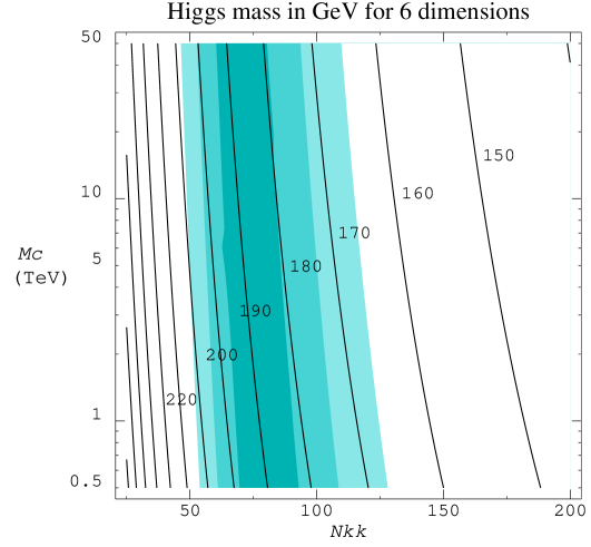
Figure 3: The predicted Higgs mass as a function of $N_{\rm KK}$ and $M_{c}$ in the six-dimensional theory with $n_{g}=1$. The shaded regions correspond to the top mass lying within 1–3 $\sigma$ (dark to light) of the experimental value, $174.3\pm 5.1$ GeV.

For six dimensions, $m=4$, $x_{H*}\approx 1.1$. The $(x_{H}-x_{H*})$ term is multiplied by a large coefficient in the RG equation, therefore it approaches zero very rapidly. Numerically we find that $\lambda_{h}/\lambda_{t}^{2}$ reaches $x_{H\ast}$ almost instantaneously below $M_{s}$. At lower energies, the $g_{3}^{2}/\lambda_{t}^{2}$ term increases and it has a large coefficient, so it is no longer a good approximation to neglect it. This term reduces $x_{H}$ in running towards low energies. If we assume that $g_{3}^{2}/\lambda_{t}^{2}$ is constant and equal to its low-energy value $g_{3}^{2}/\lambda_{t}^{2}(m_{t})$ for the correct top mass, the infrared fixed point for $x_{H}$ becomes

$$12x^{\prime}_{H\ast}+3(m-1)+\frac{64}{3}\frac{g_{3}^{2}}{\lambda_{t}^{2}}(m_{t})-\frac{6m}{x^{\prime}_{H\ast}}=0\;\;\Rightarrow\;\;x^{\prime}_{H\ast}\approx 0.5\;(\mbox{for }m=4).$$ (4.12)

Because $g_{3}^{2}/\lambda_{t}^{2}$ is smaller than $g_{3}^{2}/\lambda_{t}^{2}(m_{t})$ during the evolution, $x^{\prime}_{H*}$ provides a rough lower bound on $x_{H}$ if we ignore the difference from the SM running below $M_{c}$. Therefore, for six dimensions we expect

$$0.5\begin{array}[]{c}\,\sim\vspace{-21pt}\\ <\end{array}\frac{\lambda_{h}}{\lambda_{t}^{2}}\begin{array}[]{c}\,\sim\vspace{-21pt}\\ <\end{array}1.1,$$ (4.13)

which translates to the Higgs mass range

$$170\,{\rm GeV}\begin{array}[]{c}\,\sim\vspace{-21pt}\\ <\end{array}M_{h}=\sqrt{\lambda_{h}}v\begin{array}[]{c}\,\sim\vspace{-21pt}\\ <\end{array}260\,{\rm GeV}.$$ (4.14)

The dependence of the Higgs mass on $N_{\rm KK}$ and $M_{c}$ can also be obtained numerically, and the result is shown for six dimensions in Fig. 3. Since the top mass has been determined experimentally, we can obtain a better prediction of the Higgs mass from the measured top mass. In Fig. 3, we also show the region of the parameter space which gives the top mass within $3\sigma$ of the experimental value by the shaded area. The corresponding limit of the Higgs mass $M_{h}$ is

$$165\,{\rm GeV}<M_{h}(\mbox{6-dim})<210\,{\rm GeV}.$$ (4.15)

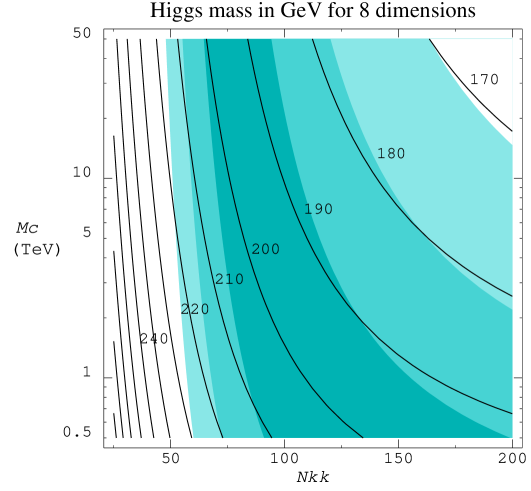
Figure 4: The predicted Higgs mass as a function of $N_{\rm KK}$ and $M_{c}$ in the eight-dimensional theory. The shaded regions correspond to the top mass lying within 1–3 $\sigma$ (dark to light) of the experimental value.

Similar Higgs mass prediction can be obtained for the eight-dimensional case. The fixed points $x_{H\ast}$ and $x^{\prime}_{H\ast}$ are $1.3$ and $0.7$ in this case, which roughly correspond to 270 GeV and 200 GeV respectively. The numerical prediction for $M_{h}$ is shown in Fig. 4.

Due to the SM running below $M_{c}$, $M_{h}$ can in fact get below 200 GeV. The predicted Higgs mass in the eight-dimensional theory from requiring a correct top mass within $3\sigma$ lies in the range

$$170\,{\rm GeV}<M_{h}(\mbox{8-dim})<230\,{\rm GeV}.$$ (4.16)

As we emphasized in the introduction, the predictions of this section have a much more general validity than our particular mechanism for triggering electroweak breaking from Standard Model gauge dynamics in extra dimensions. They are a consequence of any theory where (1) the field content is that of the Standard Model, with the gauge bosons, Higgs boson and one full generation propagating in six or eight dimensions, and (2) where the higher-dimensional couplings $\lambda_{t},\lambda_{h}$ blow up in the ultraviolet, consistent with a composite Higgs boson.

If the first two generations of fermions also propagate in extra dimensions, there may be more light bulk bound states, which can contribute to the power-law running of the top Yukawa coupling and the Higgs self-coupling. As we will discuss in the next section, some flavor breaking must be present so that only one Higgs gets a large VEV. If we simply assume that there are no new bound states even with more generations propagating in the bulk, the fixed points for $\lambda_{t}/g_{3}$ become $1.15/g_{3}(m_{t})\>(n_{g}=2)$, $1.3/g_{3}(m_{t})\>(n_{g}=3)$, for six dimensions, and $1.3/g_{3}(m_{t})\>(n_{g}=2)$, $1.5/g_{3}(m_{t})\>(n_{g}=3)$, for eight dimensions. Contributions from additional light scalars in the bulk can reduce the fixed points. Consequently, more uncertainties are introduced in the top and Higgs mass predictions, but we still expect the Higgs boson to remain rather light.

5 Flavor Symmetry Breaking

So far we have only discussed the case where the third generation of fermions propagates in $D-4$ compact dimensions, without specifying what happens with the other two generations. A possibility is that the fermions of the first two generation are four-dimensional [19], localized at some points in the space of extra dimensions. In this case, there may be (four-dimensional) bound states between the bulk fermions of the third generation and the four-dimensional fermions. The binding force of higher-dimensional scalars receives contributions from the extra components of the gauge fields, and hence is stronger than the four-dimensional ones at generic points in extra dimensions (away from the orbifold fixed points) by $D/4$ in the lowest order approximation, (as one can see from the Fierz transformations.) The discussion in the previous sections will hold if these four-dimensional bound states are indeed heavy and do not appear in the low-energy theory.

A more natural option may be that all three generations fill the $D$-dimensional spacetime, namely each of the ${\cal Q}_{+}$, ${\cal U}_{-}$, ${\cal D}_{-}$, ${\cal L}_{+}$, ${\cal E}_{-}$ fermions belongs to the fundamental representation of a global $U(3)$ symmetry. Therefore, the spacetime configuration and the Standard Model gauge interactions preserve a $U(3)^{5}$ flavor symmetry.

As we showed in sections 2 and 3, the bound state with negative squared-mass is the $\overline{\cal Q}_{+}U_{-}$ scalar, which in the case of three generations belongs to the $(3,3)$ representation of the $U(3)_{\cal Q}\times U(3)_{\cal U}$ flavor symmetry. In other words, there are nine “up-type” Higgs doublets. In the absence of flavor symmetry breaking, these Higgs doublets are degenerate and obtain VEV’s that break $U(3)_{\cal Q}\times U(3)_{\cal U}$ down to the diagonal $U(3)$, leading to eight Nambu-Goldstone bosons in addition to the ones eaten by the $W$ and $Z$. Clearly there is need for flavor breaking, not only to give sufficiently large masses to these Nambu-Goldstone bosons, but also to account for the various masses of the quarks and leptons.

We now argue that any source of flavor breaking is likely to have a large effect. Recall that the squared-mass of a composite Higgs doublet is very sensitive to the strength of the interaction between its constituents. Therefore, some perturbative, flavor non-universal interaction may easily tilt the vacuum in the direction where only one Higgs doublet has a negative squared-mass. This immediately eliminates the unwanted Nambu-Goldstone bosons.

The flavor breaking can come from operators induced at the cutoff scale $M_{s}$, such as the following four-fermion operators [3],

$$\frac{\eta_{ij}}{M_{s}^{D-2}}\left(\overline{\cal Q}_{+}^{i}{\cal U}_{-}^{j}\right)\left(\overline{\cal U}_{-}^{j}{\cal Q}_{+}^{i}\right)~{},$$ (5.1)

where $i=1,2,3$ labels the generations. If the attractive force is enhanced in one channel (identified as the 3-3 channel) relative to the others, then only one $H_{\cal U}$ (which couples to the third generation) gets a VEV, while the squared-masses of other Higgs doublets can stay positive. Note that given the sensitivity of the Higgs mass to the strength of the binding interaction, the other Higgs doublets may be quite heavy even with a small splitting in the binding strength. The flavor-changing effects induced by these scalars are small if the scalar masses are large, or the $\eta_{ij}$ coefficients approximately preserve some flavor symmetry [16].

As in any theory with quantum gravity at the TeV scale, flavor-changing effects become a problem if all possible higher-dimensional operators consistent with the SM gauge symmetry are induced with unsuppressed coefficients. One has to assume that the problematic flavor-changing operators, such as $\Delta S=2$, are suppressed by an underlying flavor symmetry or some other mechanism of the fundamental short-distance theory.

With only one or two composite Higgs doublets in the low-energy theory, the light quark and lepton masses can be generated by certain four-fermion operators induced at $M_{s}$. To be specific, let us discuss the $H_{\cal U}$ and $H_{\cal D}$ bound states. Note that even though the squared-mass of $H_{\cal D}$ is likely to be positive because the $\overline{\cal Q}_{+}^{3}{\cal D}_{-}^{3}$ channel is not sufficiently strongly coupled, a

$$\left(\overline{\cal Q}_{+}^{3}{\cal U}_{-}^{3}\right)\left(\overline{\cal Q}_{+}^{3}{\cal D}_{-}^{3}\right)$$ (5.2)

operator would induce a VEV for $H_{\cal D}$. The important point is that operators such as

$$\left(\overline{\cal Q}_{+}^{3}{\cal U}_{-}^{3}\right)\left(\overline{\cal U}_{-}^{i}{\cal Q}_{+}^{j}\right)\;,\;\;\left(\overline{\cal Q}_{+}^{3}{\cal D}_{-}^{3}\right)\left(\overline{\cal D}_{-}^{i}{\cal Q}_{+}^{j}\right)\;,\;\;\left(\overline{\cal Q}_{+}^{3}{\cal D}_{-}^{3}\right)\left(\overline{\cal E}_{+}^{i}{\cal L}_{-}^{j}\right)$$ (5.3)

induce Yukawa couplings for the Higgs doublets [18]. In fact this choice of operators has a flavor structure that leads in the low-energy theory to a type-II two-Higgs doublet model, i.e., $H_{\cal U}$ gives masses to the up-type quarks while $H_{\cal D}$ gives masses to the leptons and down-type quarks.

Another possibility to prevent the first two generation forming light bound states is that the fermions of different chirality are split in the extra dimensions [17]. Consider for example the case that quarks and leptons propagate in $D=6$ dimensions, (four infinite and two of radius $R$,) and there is one additional transverse dimension with coordinate $x^{7}$ and radius $R_{T}(>M_{s}^{-1})$ smaller than $R$. Assuming that the third generation is localized at $x^{7}=0$, and the other two generations are at $x^{7}\neq 0$ with the $+$ and $-$ chiralities localized at different $x^{7}$, the strength of the attractive channels which involve the first two generations is suppressed by the separation. In this case the spectrum of bound states is the same as the one described in section 2, namely there is a single six-dimensional Higgs doublet, $H_{\cal U}$, with a large Yukawa coupling to the top quark, and a six-dimensional Higgs doublet, $H_{\cal D}$, with a large coupling to the bottom quark (and $M_{H_{\cal D}}^{2}>M_{H_{\cal U}}^{2}$.) The light fermion masses can still arise from the operators (5.2), (5.3), with the hierarchies explained by the distances between the fermions.

6 A Comparison with Supersymmetry

Given the $SU(3)_{C}\times SU(2)_{W}\times U(1)_{Y}$ gauge structure of the quark and lepton interactions, two crucial questions arise: why is the gauge group broken spontaneously to $SU(3)_{C}\times U(1)_{EM}$, and why does just one fermion, of charge 2/3, couple strongly to this symmetry breaking. Supersymmetric extensions of the Standard Model are known to make significant progress on these questions, and in this section we compare our mechanism with the case of supersymmetric electroweak symmetry breaking.

Our extra-dimensional approach shares certain features with supersymmetric theories: both extend spacetime symmetries and have the breaking scale of this extra spacetime symmetry linked to the scale of electroweak symmetry breaking. The gauge, quark and lepton fields are extended to become representations of the larger spacetime symmetry — they propagate in superspace or in the extra-dimensional bulk. Furthermore, in both cases the dynamics which generates a negative squared mass for the Higgs field is directly connected to the interaction which leads to a heavy top quark. However, on closer inspection the mechanisms are completely different and much insight is gained by comparing the assumptions and accomplishments of these two approaches.

Perhaps the largest difference is that in supersymmetric theories the Higgs particles are added to the theory by hand, whereas in the extra-dimensional theory they are automatically generated as quark composites, bound by the Standard Model gauge forces which become strong in the bulk. It is by no means obvious that Higgs doublets need to be added in supersymmetric theories, since the scalar superpartner of the lepton doublet has the right gauge quantum numbers to be the Higgs boson. However, it has not proven possible to break electroweak symmetry using only the sneutrino VEV — one of the great “missed opportunities” of supersymmetry.

In supersymmetric theories it is very significant that the correct pattern of electroweak symmetry breaking is triggered by the radiative corrections induced by the large top quark Yukawa coupling. The theory has many scalars: squarks, sleptons and Higgs bosons, yet only the Higgs boson acquires a VEV. However, a large top quark Yukawa coupling must be input into the theory by hand. Of course, experiment tells us that the top quark is very heavy; but we would like the theory to explain why an up-type quark is heavy. It is just as easy to construct supersymmetric theories where the $\tau$ lepton has a very large Yukawa coupling rather than the top quark. In this case supersymmetry predicts a different pattern of electroweak symmetry breaking: $U(1)_{Y}$ is broken while $SU(2)$ survives as an unbroken symmetry. Thus the success of supersymmetry is to correlate the pattern of electroweak symmetry breaking with the nature of the heaviest fermion, not to explain why a fermion is heavy. Contrast this with the case that the Standard Model gauge forces propagate in 6 or 8 dimensions. There is no need to introduce an additional non-gauge interaction by hand for electroweak symmetry breaking. When the gauge forces get strong, they bind a scalar Higgs and automatically induce a large Yukawa coupling to an up-type quark. No interactions are needed beyond the Standard Model gauge forces in the extra dimensions – it is as if the gaugino interactions could somehow induce electroweak symmetry breaking and a large top quark mass! Furthermore, there is a direct link between the gauge quantum numbers of a generation and the result that the very heavy fermion is an up type quark.

While supersymmetric radiative electroweak symmetry breaking employs a heavy top quark effect, it does not predict the mass of the top quark. In fact, a very heavy top quark is not needed — 50 GeV is certainly sufficient. On the other hand, the extra-dimensional approach employs an NJL-like mechanism. In four dimensions, this would yield a large top Yukawa coupling at the compositeness scale, and unless this scale is very high (thereby necessitating an enormous fine-tune), the top quark is much too heavy, $m_{t}\approx 600$ GeV. However, the magic is that in extra dimensions, the fundamental higher-dimensional couplings can naturally be large and yet be consistent with the more “perturbative” four-dimensional couplings $g,\lambda_{t},\lambda_{h}\sim 1$ due to a moderate dilution factor from the volume of the extra dimensions. This is why our theories predict naturally smaller top and Higgs masses. In both types of theory there is the possibility that the top quark mass is determined by infrared fixed point behavior of the renormalization group equations for the Yukawa coupling. In supersymmetry, quasi-fixed-point behaviour leads to a top quark mass $m_{t}\approx 205\sin\beta$ GeV for $\tan\beta$ not too large [20]. A correct top mass can be obtained for $\tan\beta\sim 1.6$, which gives rise to a relatively light Higgs boson. The lower bound on the Higgs mass from LEP II has ruled out such a low $\tan\beta$ in the simplest Minimal Supersymmetric Standard Model. With extra dimensions, the need for criticality implies that the top quark fixed point is relevant, even though it may not be reached, and leads to a correct prediction of the top quark mass, although with considerable ${\cal O}$(20%) uncertainties. This is a very significant result. A more precise prediction is frustrated by a lack of control of the ultraviolet behavior of the theory, implying that one does not know how closely the infrared fixed point is approached. A correct prediction of the top quark mass in supersymmetric theories requires additional structure, such as $SO(10)$ grand unification; for extra dimensions, the correct prediction is inherent to the mechanism of electroweak symmetry breaking induced by the Standard Model gauge interactions.

Both schemes share a common mystery: why is there a light Higgs boson? In the supersymmetric case, once the Higgs fields have been introduced, it is necessary to understand why they do not acquire a gauge invariant mass of order the Planck scale. In the case of extra dimensions, the most natural mass for the composite scalars is of order the scale where the gauge interactions get strong, 10 TeV for example. For supersymmetry, the best solution to this “$\mu$ problem” is to introduce a symmetry which forbids a bare Higgs mass in the supersymmetric limit, and arrange for the generation of the operator $[\mu H_{\cal U}H_{\cal D}]_{F}$ once supersymmetry is broken. For extra dimensions, it is necessary to assume that the strong gauge dynamics is such as to bind the Higgs boson close to criticality, where its mass vanishes. We know of no symmetry which can guarantee this, so apparently a fine tune is necessary — this is clearly the primary weakness of the extra-dimensional scheme. Perhaps it is accidental, or perhaps it results naturally from the non-perturbative gauge dynamics which we do not understand.

For both supersymmetry and extra dimensions, given the existence of a light Higgs, the simplest schemes impose constraints on the mass of the Higgs boson. Unlike the Standard Model, the scalar quartic coupling is not a free parameter. In supersymmetric theories it is related to the electroweak gauge couplings in such a way that there is a tree level upper limit to the lightest Higgs mass of $M_{Z}$, which gets increased by radiative corrections to about 135 GeV. With dynamical electroweak symmetry breaking one typically thinks of a very heavy, or non-existent, Higgs boson. However, the extra-dimensional scheme has a light Higgs boson because the renormalization group equations of the dimensionally reduced theory has an infrared fixed point which is quickly reached, and which sets the self-coupling close to the square of the top Yukawa coupling. The expected range of the Higgs mass in the simplest scenarios is in the range 165 GeV to 230 GeV, and has no overlap with the supersymmetric case. In non-minimal theories with extra light scalars, the constraints on the Higgs mass are relaxed for both supersymmetry and extra dimensions.

In supersymmetric theories one has the freedom to add Yukawa couplings by hand to describe the full mass spectrum and mixing matrices of the quarks and charged leptons. As in the Standard Model, it is easy to construct a realistic theory of flavor — but at the expense of a deeper understanding, or any predictivity. In extra dimensions, incorporating flavor beyond the top quark mass is more challenging, and potentially more rewarding. For example, if all three generations propagate in the bulk there is a $U(3)^{5}$ flavor symmetry. The composite Higgs multiplet $H_{\cal U}$ transforms non-trivially as (3,3) under $U(3)_{Q}\times U(3)_{U}$ and, when it acquires a VEV, many of its components become Goldstone bosons. To avoid this it appears that flavor, at least in part, may be a phenomenon of the bulk. Clearly, many geometrical configurations are possible, but the crucial ingredient must be that flavor breaking is inextricably linked to spacetime symmetry breaking, which is not the situation usually envisaged in supersymmetric theories.

In both schemes, electroweak symmetry breaking is a manifestation of a deeper spacetime symmetry breaking, so that the more fundamental question becomes the origin and nature of spacetime symmetry breaking. In the case of supersymmetry, the Standard Model is protected to some degree from the primordial supersymmetry breaking, so that the question of mediating the supersymmetry breaking to the Standard Model becomes of paramount importance to phenomenology. With extra dimensions such protection is absent — the mediation of spacetime symmetry breaking to the Standard Model occurs directly via the KK spectrum of the excitations of the Standard Model particles.

In summary: extra dimensions offer a more predictive and constrained mechanism for electroweak symmetry breaking than occurs in supersymmetric theories. The Standard Model gauge interactions create a Higgs boson as a bound state of top quarks, induce it to acquire a VEV, correctly predict the top quark mass with ${\cal O}$(20%) uncertainties, and predict a somewhat light Higgs boson in the $165-230$ GeV range. It is remarkable that the puzzle of electroweak symmetry breaking may be encoded in the Standard Model gauge interactions and quantum numbers, with no need for any extra particles or interactions beyond those required by extra-dimensional propagation. Given the very plausible assumptions we have made regarding the strong Standard Model gauge dynamics, the only price to be paid is a moderate tuning to keep the composite Higgs boson light.

Acknowledgements

We would like to thank C.T. Hill, K.T Matchev, M. Schmaltz, and C.E.M. Wagner for discussions. H.-C. Cheng thanks the Theory Group at Lawrence Berkeley National Laboratory for hospitality while the work was initiated. The work of N. Arkani-Hamed and L. Hall was supported by DOE under contract DE-AC03-76SF00098 and by NSF under contract PHY-95-14797. H.-C. Cheng is supported by the Robert R. McCormick Fellowship and by DOE Grant DE-FG02-90ER-40560. B.A. Dobrescu is supported by DOE Grant DE-AC02-76CH03000.

Appendix:  Vector-like Fermions

In this Appendix we consider the case where the higher-dimensional fermions are vector-like. This is always the case when the number of dimensions accessible to the fermions, $D$, is odd, but it also occurs as a particular case for even $D$.

Vector-like $D$-dimensional fermions may form all the bound states discussed in section 2 as well as new ones. In particular, the most attractive channel is the gauge-singlet scalar made of $\overline{{\cal Q}}{\cal Q}$. $H_{\cal U}=\overline{{\cal Q}}{\cal U}$ is still the most attractive channel which transforms non-trivially under the SM gauge group, but it is less strongly bound than the singlets $S_{\cal Q}=\overline{{\cal Q}}{\cal Q}$ and $S_{\cal U}=\overline{{\cal U}}{\cal U}$. Assuming $\hat{g}_{3}=\hat{g}_{2}=\hat{g}_{1}$, the $S_{\cal Q}$ and $S_{\cal U}$ channels are stronger than $H_{\cal U}$ by $3/2$ and $8/7$ respectively, and hence will likely condense first. The VEV’s of these singlets do not break any gauge symmetry. However, they give positive squared-mass to the Higgs, $H_{\cal U}$, through their cross interactions, (or equivalently, dynamical masses to the constituents of the Higgs, $Q$, $U$.) This may prevent the Higgs from acquiring a VEV, jeopardizing the simple mechanism for electroweak symmetry breaking. It is a detailed question whether the Higgs can still acquire a nonzero VEV in the presence of these singlets, and it is hard to be estimated reliably with simple approximations.

One thing which can help electroweak symmetry breaking to occur is the orbifold projection required to obtain the four-dimensional chiral theory. Let us demonstrate it by an example with a simple setup. Assuming that each higher-dimensional fermion has $2^{n+1}$ components, we can obtain a single four-dimensional chiral zero mode by incorporating orbifold projections with $n$ ${\bf Z}_{2}$ symmetriess, with the composite scalars $\overline{{\cal Q}}{\cal Q}$ and $\overline{{\cal U}}{\cal U}$ being odd under all $n$ ${\bf Z}_{2}$ symmetries. (By contrast, $H_{\cal U}=\overline{{\cal Q}}{\cal U}$ is even under all ${\bf Z}_{2}$’s.) After decomposed into four-dimensional KK modes, $S_{\cal Q}$ and $S_{\cal U}$ have no zero modes, and their lowest modes will have a KK mass component of $\sqrt{n}/R$, which makes their squared-masses less negative. In addition, their self-quartic-couplings will be enhanced by $(3/2)^{n}$, because their wave functions are proportional to the Sine function in these $n$ directions and $\int_{0}^{2\pi R}dy(\sqrt{2}\sin y/R)^{4}=3/2$. Larger self-couplings and less negative squared-masses result in smaller VEV’s for $S_{\cal Q}$ and $S_{\cal U}$ and smaller contributions to the squared-mass of ${\cal H_{U}}$. Based on the simplest one-loop effective potential estimate, one finds that for $n>2$, the Higgs can still develop a nonzero VEV and break the electroweak symmetry.

Although this analysis is hardly reliable and depends on how the extra dimensions are compactified and the four-dimensional chiral fermions are obtained, it shows that dynamical electroweak symmetry breaking is not ruled out in this scenario. If electroweak symmetry breaking does occur correctly, the low-energy theory will contain two Higgs doublets, a color-triplet scalar $\tilde{b}=\overline{{\cal Q}}{\cal Q}^{c}$ discussed in section 2.2, and several gauge-singlet scalars, $S_{\cal Q}=\overline{{\cal Q}}{\cal Q}$, $S_{\cal U}=\overline{{\cal U}}{\cal U}$, and $S_{\cal D}=\overline{{\cal D}}{\cal D}$.

References

-
[1]
N. Arkani-Hamed, S. Dimopoulos and G. Dvali,
“The Hierarchy problem and new dimensions at a millimeter,”
Phys. Lett. B429, 263 (1998)
hep-ph/9803315;
I. Antoniadis, N. Arkani-Hamed, S. Dimopoulos and G. Dvali, “New dimensions at a millimeter to a Fermi and superstrings at a TeV,” Phys. Lett. B436, 257 (1998) hep-ph/9804398. -
[2]
L. Randall and R. Sundrum,
“A Large mass hierarchy from a small extra dimension,”
hep-ph/9905221;
N. Arkani-Hamed, S. Dimopoulos, G. Dvali and N. Kaloper, “Infinitely large new dimensions”, hep-th/9907209;
J. Lykken and L. Randall, “The Shape of gravity,” hep-th/9908076. - [3] B.A. Dobrescu, “Electroweak symmetry breaking as a consequence of compact dimensions,” Phys. Lett. B461, 99 (1999) hep-ph/9812349.
- [4] H.-C. Cheng, B. A. Dobrescu and C. T. Hill, “Electroweak symmetry breaking and extra dimensions,” hep-ph/9912343.
- [5] N. Arkani-Hamed and S. Dimopoulos, “New origin for approximate symmetries from distant breaking in extra dimensions,” hep-ph/9811353.
-
[6]
Y. Nambu,
“BCS Mechanism, Quasi Supersymmetry, And Fermion Masses”,
in the Proceedings of the
XI Warsaw Symposium on Elementary Particle Physics, May 1988,
ed. Z. Ajduk, et al (World Scientific, 1989); “Quasisupersymmetry, Bootstrap Symmetry Breaking And Fermion Masses,”
in the Proceedings of the 1988 International Workshop on New Trends in
Strong Coupling Gauge Theories, Nagoya, Japan, ed. M. Bando, T.Muta
and K. Yamawaki
(World Scientific, 1989); “Bootstrap Symmetry Breaking In Electroweak Unification”,
EFI-89-08 (1989);
V.A. Miransky, M. Tanabashi and K. Yamawaki, Mod. Phys. Lett. A4, 1043 (1989); Phys. Lett. B221, 177 (1989);
W.J. Marciano, Phys. Rev. Lett. 62, 2793 (1989). - [7] W.A. Bardeen, C.T. Hill and M. Lindner, “Minimal Dynamical Symmetry Breaking Of The Standard Model,” Phys. Rev. D41, 1647 (1990).
- [8] M. B. Green and J. H. Schwarz, “Anomaly Cancellations In Supersymmetric D = 10 Gauge Theory Require SO(32),” Phys. Lett. B149, 117 (1984).
- [9] Y. Nambu and G. Jona-Lasinio, “Dynamical model of elementary particles based on an analogy with superconductivity. I,” Phys. Rev. 122, 345 (1961).
- [10] S. Raby, S. Dimopoulos and L. Susskind, “Tumbling Gauge Theories,” Nucl. Phys. B169, 373 (1980).
- [11] K.R. Dienes, E. Dudas and T. Gherghetta, “Extra spacetime dimensions and unification,” Phys. Lett. B436, 55 (1998) hep-ph/9803466.
- [12] H.-C. Cheng, B.A. Dobrescu and C.T. Hill, “Gauge coupling unification with extra dimensions and gravitational scale effects,” hep-ph/9906327.
- [13] R.S. Chivukula, B.A. Dobrescu, H. Georgi and C.T. Hill, “Top quark seesaw theory of electroweak symmetry breaking,” Phys. Rev. D59, 075003 (1999) hep-ph/9809470.
- [14] C. Caso et al., “Review of particle physics,” Eur. Phys. J. C3, 1 (1998), and 1999 Web update, http://pdg.lbl.gov.
-
[15]
C. T. Hill,
“Quark And Lepton Masses From Renormalization Group Fixed Points,”
Phys. Rev. D24, 691 (1981);
B. Pendleton and G. G. Ross, “Mass And Mixing Angle Predictions From Infrared Fixed Points,” Phys. Lett. B98, 291 (1981);
S. A. Abel and S. F. King, “On fixed points and fermion mass structure from large extra dimensions,” Phys. Rev. D59, 095010 (1999), hep-ph/9809467. - [16] H. Georgi and A. K. Grant, “A topcolor jungle gym,” hep-ph/0006050.
- [17] N. Arkani-Hamed and M. Schmaltz, “Hierarchies without symmetries from extra dimensions,” hep-ph/9903417.
- [18] B. A. Dobrescu, “Minimal composite Higgs model with light bosons,” hep-ph/9908391.
- [19] C.D. Carone, “Electroweak constraints on extended models with extra dimensions,” Phys. Rev. D61, 015008 (2000) hep-ph/9907362.
-
[20]
M. Carena, T. E. Clark, C. E. Wagner, W. A. Bardeen and K. Sasaki,
“Dynamical symmetry breaking and the top quark mass in the minimal
supersymmetric standard model,”
Nucl. Phys. B369, 33 (1992);
W. A. Bardeen, M. Carena, S. Pokorski and C. E. Wagner, “Infrared fixed point solution for the top quark mass and unification of couplings in the MSSM,” Phys. Lett. B320, 110 (1994), hep-ph/9309293;
M. Carena, M. Olechowski, S. Pokorski and C. E. Wagner, “Radiative electroweak symmetry breaking and the infrared fixed point of the top quark mass,” Nucl. Phys. B419, 213 (1994), hep-ph/9311222.