A Study on
the Non-perturbative Existence of Yang-Mills Theories
with
Large Extra Dimensions

Abstract

Pure lattice $SU(2)$ Yang-Mills theory in five dimensions is considered, where an extra dimension is compactified on a circle. Monte-Carlo simulations indicate that the theory possesses a continuum limit with a non-vanishing string tension if the compactification radius is smaller than a certain value $R_{M}$ which is $O(1/10)$ of the inverse of the square root of the string tension. We verify non-perturbatively the power-law running of gauge coupling constant. Our method can be applied to the investigation of continuum limits in other higher-dimensional gauge theories.

I INTRODUCTION

The idea of unifying fundamental forces by introducing extra dimensions has attracted attention for many decades, and a theory realizing this idea is called Kaluza-Klein theory [1].

Recently, it has been observed by Arkani-Hamed, Dimopoulos and Dvali [2] that the existence of extra dimensions may play an important rôle to understand the hierarchical scales that exist between the weak and Planck scales. From a simple setting that only the graviton can propagate in the bulk corresponding to the extra dimensions while all the other fields of the Standard Model (SM) are located on a four-dimensional wall, they have concluded [2] that the length scale of the extra dimensions can be rather large $\mathrel{\mathchoice{\vbox{\offinterlineskip\halign{$\m@th\displaystyle\hfil#\hfil$\cr>\crcr\sim\crcr} }}{\vbox{\offinterlineskip\halign{$\m@th\textstyle\hfil#\hfil$\cr>\crcr\sim\crcr} }}{\vbox{\offinterlineskip\halign{$\m@th\scriptstyle\hfil#\hfil$\cr>\crcr\sim\crcr} }}{\vbox{\offinterlineskip\halign{$\m@th\scriptscriptstyle\hfil#\hfil$\cr>\crcr\sim\crcr} }}}10^{-2}$ cm, in contrast to previously suggested Kaluza-Klein theories in which the size of extra dimensions was of the order of the (four-dimensional) Planck length $10^{-33}$ cm or $1/M_{\rm GUT}\approx 10^{-30}$ cm, where $M_{\rm GUT}$ is the unification scale in four-dimensional grand unified theories (GUTs). Their idea has been then followed and extended by several authors [3, 4] to obtain more satisfying solutions of the hierarchy problem. Moreover, the above phenomenological proposal to confine fields on a lower-dimensional subspace fits well [6, 7, 8, 9] the D-branes [5] (extended objects attached by the end points of open strings) in string theories.

If part of the SM fields can propagate in the bulk, and the size of the extra dimensions are large, the existence of such extra dimensions may be experimentally verified. There will be a number of phenomenological questions (see [10] for instance) like “ what are the experimental bounds on the size of the extra dimensions? [11]” However, our concern in this paper is of a theoretical nature: Is the existence of a large extra dimension consistent with quantum theory? Our answer to this question will be “Yes”, provided that the compactification radius $R$ is smaller than a certain value, the maximal radius $R_{M}$. It should be emphasized that the previous investigations [12, 13, 14] on non-abelian gauge theories in five dimensions on a lattice (which indicated that the theory have no continuum limit) were performed in the uncompactified case. These works [13, 14] were motivated to investigate whether or not the non-trivial ultraviolet fixed point found in the $\epsilon$-expansion [15] is real.

To be more specific, we consider pure $SU(2)$ Yang-Mills theory in five dimensions where an extra dimension is compactified on a circle $S$ with the radius of $R$. (It would be more “realistic” to compactly the fifth dimension on the orbifold $S/Z_{2}$ so that the zero-modes contain only four-dimensional gauge fields and no scalar fields. We leave the case of $S/Z_{2}$ to future work.) One may expect that the theory will carry the basic property of a four-dimensional gauge theory if the radius $R$ is sufficiently small, while in the opposite limit of $R$ the theory becomes more five dimensional. So there may be the maximal radius $R_{M}$ below which the theory can possess a continuum limit with a non-vanishing string tension and can exist non-perturbatively. We will indeed find that our numerical simulations based on a compactified lattice gauge theory are supporting the correctness of this heuristic picture.

The string tension is one of the most familiar physical quantities, which can give a physical scale to the lattice spacing. However, at a deconfining phase transition of first order, the string tension vanishes discontinuously, and we cannot use it for that purpose in this case. One of the crucial observations in this paper is that, if the fifth dimension is compactified, the first order phase transition changes its nature at a certain compactification radius. We will see this on anisotropic lattices by performing Monte-Carlo simulations with various compactification radii and by investigating the phase structure. The simulations also indicate that it could be possible to give a physical scale to the lattice spacing even in the deconfining phase if the theory is compactified, and this possibility will be studied more in detail.

We will assume that the phase transition due to the compactification occurs at a certain value of $R$, the critical compactification radius $R_{C}$, and that the compactification radius is kept fixed at $R_{C}$ along the critical line of the phase transition due to the compactification. That is, the critical compactification radius $R_{C}$ is assumed to be a physical quantity. This assumption enables us to compute the lattice $\beta$-function for a given $R$ as a function of the lattice spacing $a_{4}$ of the four-dimensional direction. In doing so, we can verify non-perturbatively the power-law running of the gauge coupling constant $g$, and find that the observed power law behavior fits well to the one-loop form suggested in Refs. [8, 15, 16, 17, 18, 19, 20, 21, 22]. The results for the lattice $\beta$-function obtained from our Monte-Carlo simulations indicate the self-consistency of the assumption above.

The results obtained for the lattice $\beta$-function can also be used to make a further assumption on the physical scale in the deconfining phase and to investigate various scaling properties of the longitudinal Creutz ratio (defined in Eq. (17)), making a discussion on the existence of continuum limits of the theory possible. We will be led to the interpretation that the theory may possess a continuum limit with a non-vanishing longitudinal string tension if the compactification radius $R$ is smaller than $R_{M}\approx R_{C}/3$, and that the non-trivial ultraviolet fixed point found in the $\epsilon$-expansion in the continuum theory may no longer be spurious.

After we define our lattice action in Section II, we start to present the details of our calculations. In Section III we calculate the ratio of the lattice spacings $\xi=a_{4}/a_{5}$ in terms of the parameters of the simulations $\beta$ and $\gamma$, and then we discuss the phase structure in Section IV. In Section V we compute the lattice $\beta$-function and then study on a continuum limit in Section VI, and the last Section is devoted for conclusion.

II THE ACTION

In order to investigate the effects of a compactification in the 5-dimensional $SU(2)$ gauge theory, it is crucial to employ an anisotropic lattice which has different lattice spacings, $a_{4}$ and $a_{5}$, in the four-dimensional directions and in the fifth direction, and is often used in the case of lattice gauge theories at finite temperature. We find that the effects of the compactification on an isotropic lattice can appear only for a small lattice size of the fifth direction $(\leq 2)$ so that it is practically impossible to study the theory with different sizes of this direction. Another advantage is that, since we can vary $a_{4}$ and $a_{5}$ independently, we can investigate the $a_{4}$ dependence of physical quantities while keeping $a_{5}$ fixed. This enables us to study scaling properties in the compactifed theory for a given compactification radius $R$.

We denote the five-dimensional lattice coordinates by $z_{M}~{}(M=1,\dots,5)$ while the four-dimensional ones by $x_{\mu}~{}(\mu=1,\dots,4)$ and the fifth one by $y$. Link variable takes the form

$$U_{M}(x,y) = \{~{}U_{\mu}(x,y)=U(x,y;x+a_{4}\hat{\mu},y)~{},~{}U_{5}(x,y)=U(x,y;x,y+a_{5})~{}\}~{},$$ (1)

where $U(z_{1};z_{2})\in SU(N_{C})$ is the parallel transporter. The plaquette variables are

$$U_{P_{4}} = U_{\mu\nu}(x,y)=U_{\mu}(x,y)U_{\nu}(x+a_{4}\hat{\mu},y)U_{\mu}^{{\dagger}}(x+a_{4}\hat{\nu},y)U_{\nu}^{{\dagger}}(x,y)$$ (2)

$$U_{P_{5}} = U_{\mu 5}(x,y)=U_{\mu}(x,y)U_{5}(x+a_{4}\hat{\mu},y)U_{\mu}^{{\dagger}}(x,y+a_{5})U_{5}^{{\dagger}}(x,y)~{}.$$ (3)

The Wilson action for pure $SU(N_{C})$ Yang-Mills theory in five dimensions is given by

$$S = \beta_{4}~{}\sum_{P_{4}}~{}[~{}1-\frac{1}{N_{C}}~{}\mbox{Re Tr}~{}U_{P_{4}}~{}]+\beta_{5}~{}\sum_{P_{5}}~{}[~{}1-\frac{1}{N_{C}}~{}\mbox{Re Tr}~{}U_{P_{5}}~{}]~{},$$ (4)

where $\sum_{P_{4}}=\sum_{z~{}1\leq\mu<\nu\leq 4}$ and $\sum_{P_{5}}=\sum_{z~{}1\leq\mu\leq 4}$. Periodic boundary conditions are imposed in all the directions. The coupling- and correlation-anisotropy parameters are defined as

$$\gamma = \sqrt{\frac{\beta_{5}}{\beta_{4}}}~{},~{}\xi=\frac{a_{4}}{a_{5}}~{},$$ (5)

where $\gamma=\xi$ is satisfied in the tree level. In the naive continue limit $a_{4},a_{5}\to 0$ with the length of the fifth dimension fixed at $2\pi R$, the action (4) becomes

$$S = -\sum_{x,y}~{}[~{}(\frac{\beta_{4}a_{4}^{4}}{2N_{C}})~{}\frac{1}{2}\mbox{Tr}F_{\mu\nu}^{2}+~{}(\frac{\beta_{5}a_{4}^{2}a_{5}^{2}}{2N_{C}})~{}\mbox{Tr}F_{5\nu}^{2}~{}]+O(a^{5})~{},$$ (6)

which goes to

$$\int d^{4}x\int_{0}^{2\pi R}dy~{}\frac{-1}{2g_{5}^{2}}~{}\mbox{Tr}F_{MN}^{2}~{},$$ (7)

if $\beta_{4}=2N_{C}a_{5}/g_{5}^{2}$ and $\beta_{5}=2N_{C}a_{4}^{2}/g_{5}^{2}a_{5}$, where $A_{M}=g_{5}A_{M}^{a}T^{a}~{},~{}F_{MN}=\partial_{M}A_{N}-\partial_{N}A_{M}-i[~{}A_{M}~{},~{}A_{N}~{}]$, and we have used

$$U_{\mu}(x,y) = e^{ig_{5}a_{4}A_{\mu}(x,y)}~{},~{}U_{5}(x,y)=e^{ig_{5}a_{5}A_{5}(x,y)}~{}.$$ (8)

On a lattice we mean a compactification if

$$\frac{N_{4}a_{4}}{N_{5}a_{5}} = \frac{a_{4}N_{4}}{2\pi R}=\frac{N_{4}}{N_{5}}~{}\xi>1$$ (9)

is satisfied. Note that the gauge coupling constant $g_{5}$ has the dimension of $\sqrt{a_{4}}$, and can be expressed as

$$g_{5}^{-2} = \frac{\beta}{2N_{C}a_{4}}~{},~{}\beta=\sqrt{\beta_{4}\beta_{5}}~{}.$$ (10)

Later on we will use a dimensionless coupling constant $g$,

$$g^{-2} = (2\pi R)g_{5}^{-2}=\frac{N_{5}\beta}{2N_{C}\xi}~{},$$ (11)

which is normalized for the four-dimensional Yang-Mills theory with the tower of the Kaluza-Klein excitations. At this point, Eq. (11) is only a tree-level definition.

III $\xi$–$\gamma$ RELATION

The parameters of the simulations are $\beta$ and $\gamma$ for a given size of lattice, and the lattice spacings $a_{4}$ and $a_{5}$ are functions of these parameters. The introduction of an anisotropy into a lattice means that the regularization breaks $O(5)$ invariance of the continuum theory. To recover this symmetry we have to fine tune the anisotropy parameters $\gamma$ and $\xi$ that are defined in Eq. (5). At the tree-level, it is $\xi=\gamma$ as we have stated in the previous section. In higher orders the tree-level relation suffers from quantum corrections so that it can depend on $\beta$ and $\gamma$, i.e., $\xi=\xi(\gamma,\beta)$. The basic idea to find the corrected relation, which has been intensively used in the study of QCD at finite temperature, is to use that symmetry. There are variants of the method, and we have decided to use a slightly modified method that is based on the matching of the Wilson loop ratio [23, 24, 25]. Let us briefly explain the method below.

We consider two kinds of Wilson loops $W(z_{M},z_{N})$, the one $W(x_{\mu},x_{\nu})$ within the four-dimensional subspace and the other one $W(x_{\mu},y)$ that is extended into the fifth dimension, and calculate the ratios

$$R(x_{\mu},x_{\nu}) = \frac{W(x_{\mu}+a_{4}\hat{\mu},x_{\mu})}{W(x_{\mu},x_{\nu})}~{}~{}\mbox{and}~{}~{}R(x_{\mu},y)=\frac{W(x_{\mu}+a_{4}\hat{\mu},y)}{W(x_{\mu},y)}\ .$$ (12)

Since the Wilson loop is related to the static quark potential as

$$W(z_{M},z_{N})\sim\exp\{-z_{M}V(z_{N})\}~{}~{}\mbox{ ~{}~{}~{}for $z_{M}\rightarrow\infty$}~{},$$ (13)

we find that the rations (12) for large $x$ and $y$ become

$$R(x_{\mu},x_{\nu}) \sim \exp\{-a_{4}V(x_{\nu})\}\ ,~{}R(x_{\mu},y)\sim\exp\{-a_{4}V(y)\}\ .$$ (14)

The $O(5)$ symmetry of the continuum theory requires then that

$$R(x_{\mu},x_{\nu})=k~{}R(x_{\mu},y)~{}~{}\mbox{for}~{}~{}x_{\nu}=n_{\nu}a_{4}=y=n_{5}a_{5}~{},$$ (15)

where we have allowed the presence of the factor $k$. We measure the ratios for a given set of the lattice size, $\beta$ and $\gamma$, and assume that they take the form

$$R(x_{\mu},a_{4}n_{\nu}) \sim k_{1}\exp\{-\sigma_{4}n_{4}\}~{}~{}\mbox{and}~{}~{}R(x_{\mu},a_{5}n_{5})\sim k_{2}\exp\{-\sigma_{5}n_{5}\}\ ,$$ (16)

and that they should become identical with each other, by symmetry, when $n_{\nu}a_{4}=n_{5}a_{5}$. From this consideration we obtain $\xi=a_{4}/a_{5}=\sigma_{4}/\sigma_{5}$. Note that the ansatz (16) has a meaning only in the confining region of the parameters, of course.

In the practice, we fit the ansatz (16) for the data, and then scale $n_{5}$ by $z$ (i.e. $n_{5}\to zn_{4}$) in such a way that $R(x_{\mu},za_{5}n_{4})$ becomes closest to $R(x_{\mu},a_{4}n_{4})$, where we assume that $k=1$ on the r.h.side of Eq. (15) . In the ideal case we would have $z=\sigma_{1}/\sigma_{2}=\xi$.

To restore the $O(5)$ symmetry in an efficient way, simulations are performed using the heat bath algorithm of the $SU(2)$ lattice gauge theory. We employ a lattice of $N_{4}^{4}\times N_{5}$ shown in TABLE I, where $N_{5}\sim\gamma N_{4}$ is satisfied. We generate 5000 configurations, and Wilson loops are measured every 5 configurations.

Fig. 1 shows $\xi$ versus $\beta$ for various values of $\gamma$, and we see that $\xi$ is almost independent of $\beta$. The data points for larger $\beta$ are not plotted because they correspond to the deconfining region so that the ansatz (16) has no meaning. The same data are plotted in Fig. 2 which shows the $\gamma$ dependence of $\xi$. The data are summarized in TABLE I. The central value of $\xi$ in the table is the average of the data points in Fig. 1 for a fixed $\gamma$.

IV PHASE STRUCTURE

In this section we would like to investigate the phase structure of the five-dimensional theory defined by the action (4). It is known from the mean field analysis that higher-dimensional lattice gauge theories in more than four dimensions have a first order phase transition . The studies of Monte-Carlo simulations [12, 13] also indicate that in the case of $SU(2)$ gauge theory the first order transition occurs starting at $D=5$. Our task is to extend these analyses to the compactified theory. To this end, we will be intensively using anisotropic lattices to take into account the compactification of the fifth dimension.

A Longitudinal Creutz ratio

The string tension between two quarks that are separated in space is a typical physical quantity for the theory. What we know from experiments is that the string tension $\sigma_{\rm phys}$ between two quarks that are separated in the four-dimensional subspace should be non-vanishing so that the potential between them is linearly increasing with the distance $r$. And the string tension is a good physical quantity to introduce a physical scale for other quantities obtained by a lattice calculation. If the underlying gauge theory is formulated in five dimensions, however, the feature of the linearly increasing potential is not automatically present, and in fact, the first order deconfining transition is found in Refs. [12, 13].

We measure the Creutz ratio $\chi(i,j)$ defined as

$$\chi(i,j) = -\ln\{\frac{W(i,j)W(i-1,j-1)}{W(i,j-1)W(i-1,j)}\}~{},$$ (17)

where $W(i,j)$ is a rectangular Wilson loop with lengths of $i$ and $j$. The Creutz ratio with large $i$ and $j$ becomes the lattice string tension $\sigma_{\rm lat}$ in the case of the linearly increasing potential between two quarks. So, if a Creutz ratio with large $i$ and $j$ takes a non-zero value, the corresponding Wilson loop shows the area law which we regard as “confinement”. We consider the Wilson loops longitudinal to the four-dimensional subspaces, because we are interested in the confinement property in this subspace. We would like to demonstrate that the Creutz ratio behaves differently for different types of lattice. The results obtained from Monte-Carlo simulations on an isotropic lattice of size $8^{5}$ ($\gamma^{2}=1.0$) and on an anisotropic lattice of the same size ($\gamma^{2}=2.0$ and $\gamma^{2}=4.0$) are shown in Fig. 3, where the vertical axis stands for the Creutz ratio, and the horizontal axis stands for $\beta=\sqrt{\beta_{4}\beta_{5}}$. We have generated 2500 configurations for each simulation point after thermalization, and Wilson loops are measured every 5 configurations for the calculation of the Creutz ratio.

We see from Fig. 3 that the phase transition between the confining and deconfining phase exists around $\beta=1.64$ in the case of the isotropic lattice ($\gamma^{2}=1.0$) as it was found in Refs. [12, 13] and around $\beta\approx 1.73$ and $1.77$ in the cases of $\gamma^{2}=2.0$ and $4.0$, respectively. We have performed the simulations starting with an ordered configuration with $U_{M}=1$ (defined in Eq. (1)) and with a disordered configuration, thereby obtaining clear hysteresis curves. The open symbols are the results of the ordered start and the filled symbols are those of the disordered start. Our results indicate that the transitions are of first order, in accord with the finding of Refs. [12, 13] for $\gamma^{2}=1.0$.

B Transverse Polyakov loop

In the uncompactified case, the Polyakov loop plays the rôle for an indicator of confinement. Here we consider loops which are transverse to the four-dimensional subspace and define the transverse Polyakov loop as

$$L = z\frac{1}{N_{4}^{4}}\sum_{x}\frac{1}{N_{C}}{\rm Tr}\prod_{y}U_{5}(x,y)~{},$$ (18)

where $z$ is a $Z(N_{C})$ phase factor ($z^{N_{C}}=1$) such that $\arg(L)\in(-\pi/N_{C},\pi/N_{C})$. In contrast to the longitudinal Creutz ratio (17) which we have discussed in the previous subsection, the transverse Polyakov loop (18) has no direct physical meaning in four dimensions, because we do not identify the fifth direction with the temporal direction. We may say however that the quark currents running into the fifth direction are confined if the transverse Polyakov loop $\langle L\rangle$ vanishes.

Fig. 4 shows the results of the transverse Polyakov loop on the $8^{5}$ and $8^{4}\times 12$ lattices for various values of $\gamma$, while, for comparison, the average of the plaquettes ($1\times 1$ Wilson loop) for the same lattices is shown in Fig. 5. 2500 configurations have been used to measure the Polyakov loop and the plaquette for each point. As in the previous subsection, the open symbols are the results of the ordered start and the filled symbols are those of the disordered start. As expected, we obtain clear hysteresis curves, and so the transverse Polyakov loop and the average of the plaquettes also indicate that the phase transition is of first order.

C Compactification effects

It may be worth pointing out that the compactified $(D+1)$-dimensional $SU(N_{C})$ lattice gauge theory belongs to the same universality class as the $D$-dimensional $Z(N_{C})$ spin model. The case of QCD at finite temperature $T$ is a well-known example, where the temporal direction is compactified with the length $T^{-1}$. We expect the existence of a similar phase transition due to the compactification in our case, which is of second order, because the phase transition in the four-dimensional $Z(2)$ spin model (Ising model) is of second order. So, we repeat the measurements of the transverse Polyakov loop (18) and the average of plaquette for the compactified case.

In order to take into account the compactification of the fifth-dimension, we use anisotropic lattices of size $8^{4}\times 4$ and $8^{4}\times 6$. The results for the transverse Polyakov loop with different $\gamma$ are shown in Fig. 6 and 7. (In Fig. 6 we have included the result on a $12^{4}\times 4$ lattice which shows that there are practically no finite size effects.) Noticing that the compactification radius $R$($=N_{5}a_{5}/2\pi$) becomes smaller for a given $N_{5}$ as $\gamma$ becomes larger (see Fig. 2 and TABLE I), we observe that the nature of the phase transition changes due to the compactification. Namely, the interval of $\beta$ in which two phases coexist becomes narrower as $\gamma$ increases, and there are no intervals for $\gamma^{2}\mathrel{\mathchoice{\vbox{\offinterlineskip\halign{$\m@th\displaystyle\hfil#\hfil$\cr>\crcr\sim\crcr} }}{\vbox{\offinterlineskip\halign{$\m@th\textstyle\hfil#\hfil$\cr>\crcr\sim\crcr} }}{\vbox{\offinterlineskip\halign{$\m@th\scriptstyle\hfil#\hfil$\cr>\crcr\sim\crcr} }}{\vbox{\offinterlineskip\halign{$\m@th\scriptscriptstyle\hfil#\hfil$\cr>\crcr\sim\crcr} }}}2$ for the $8^{4}\times 4$ case and for $\gamma^{2}\mathrel{\mathchoice{\vbox{\offinterlineskip\halign{$\m@th\displaystyle\hfil#\hfil$\cr>\crcr\sim\crcr} }}{\vbox{\offinterlineskip\halign{$\m@th\textstyle\hfil#\hfil$\cr>\crcr\sim\crcr} }}{\vbox{\offinterlineskip\halign{$\m@th\scriptstyle\hfil#\hfil$\cr>\crcr\sim\crcr} }}{\vbox{\offinterlineskip\halign{$\m@th\scriptscriptstyle\hfil#\hfil$\cr>\crcr\sim\crcr} }}}4$ for the $8^{4}\times 6$ case, respectively. These phase transitions seem to be of second order. Observe also that the transition interval of $\beta$ for $\gamma^{2}=1.0$ does not depend on $N_{5}$, while, in contrast to this, the transition point $\beta_{C}$ for the second order transition for a given $\gamma$ depends on $N_{5}$. From these results, we conclude that the second order phase transition is caused by the compactification, and that the first order transition is not related to the compactification. In Figs. 8 and 9, we plot the average of the plaquettes for the $8^{4}\times 4$ and $8^{4}\times 6$ lattices. The results show that the transition becomes weak (like a cross over transition) starting at $\gamma$ at which the first order transition of the transverse Polyakov loop turns to be of second order. (In Fig. 8 we have included the result on a $12^{4}\times 4$ lattice to make it sure that finite size effects are negligible.)

In Fig. 10 we show the qualitative nature of the phase structure in the $\beta_{4}-\beta_{5}$ plane, which we have obtained from the result of this section. The “confining” and “deconfining” phases are separated by the critical lines of the first and second order phase transitions. The position of the critical line (bold line) of the first order phase transition does not depend on the lattice size, while that of the second order one (solid line) depends crucially on $N_{5}$. Below the critical line in the $\beta_{4}-\beta_{5}$ plane, the transverse Polyakov loop vanishes, and it is different from zero above the line. Note that this does not necessarily mean that the longitudinal Creutz ratio (17) vanishes in the deconfining phase. The longitudinal Creutz ratio (17) corresponds to the ”spatial string tension” in QCD at finite temperature, which is defined by the spatial Wilson loop, and indeed is non-vanishing even in the deconfining phase [27]. Fig. 11 shows the longitudinal Creutz ratio versus $\beta$ for the anisotropic lattice of size $8^{4}\times 4$ with $\gamma^{2}$ fixed at $4.0$. The figure shows that the longitudinal Creutz ratio varies smoothly as $\beta$ enters into the deconfining phase of the transverse Polyakov loop, indicating that it could be possible to give a physical scale to the lattice spacing even in that phase. Since indeed the spatial string tension is known to obey a scaling law at high temperature [27], we may wonder whether some continuum limit in the present might also exist. The following subsections and sections are devoted to investigate this possibility from another point of view.

In the case of QCD at finite temperature, the critical temperature $T_{C}$ is a physical quantity. As in that case, it is well possible that the critical compactification radius $R_{C}$ is a physical quantity, and that the lattice system on the different critical lines in the $\beta-\gamma$ plane for different $N_{5}$ corresponds to the same physical system. As a first check, we estimate roughly the critical radius $R_{C}$ for two critical lines of the second order phase transition at the end point. As mentioned (see also Fig. 16), at $\gamma\approx\sqrt{2.0}$ for $N_{5}=4$ and at $\gamma\approx 2.0$ for $N_{5}=6$, the second order transition line merges in the first order transition line. The value of $\xi$ at the merging points, respectively, is $1.78$ for $\gamma=\sqrt{2.0}$ and $2.78$ for $\gamma=2.0$, where we have used the data in TABLE I. From the data on the Creutz ratio for the $8^{5}$ lattice (Fig. 3), we find that the value of the longitudinal Creutz ratio at the transition points is approximately constant independent of $\gamma$, i.e.

$$\sigma_{\rm lat} = \sigma_{\rm phys}a^{2}_{4}\approx 0.7~{},$$ (19)

where we identify the longitudinal Creutz ratio $\chi(i,j)$ with large $i$ and $j$ as the lattice string tension $\sigma_{\rm lat}$. Using this, we find

$$R_{C} = \frac{N_{5}a_{5c}}{2\pi}\approx\frac{N_{5}}{2\pi\xi_{c}}~{}\left[\frac{0.7}{\sigma_{\rm phys}}\right]^{1/2}\approx\left\{\begin{array}[]{l}0.30/\sqrt{\sigma_{\rm phys}}\\ 0.29/\sqrt{\sigma_{\rm phys}}\end{array}\right.~{}~{}\mbox{ for}~{}~{}\left\{\begin{array}[]{l}N_{5}=4\\ N_{5}=6\end{array}\right.~{},$$ (24)

where $\xi_{c}=a_{4}/a_{5c}$. These values are consistent with the assumption that the lattice system on the different critical lines corresponds to the same physical system. Eq. (19) also means that the value of $a_{4}$ at which the first order phase transition appears is approximately independent of $\gamma$, indicating that this value might have a sensible meaning. In the next section, we will do another check by using the lattice $\beta$-function.

V THE LATTICE $\beta$-FUNCTION

We are interested in the physics in the four-dimensional subspace with a certain compactification radius. The anisotropic lattice we have used in the previous section is convenient for computations with different $a_{4}$ while keeping the compactification radius constant. In this section we would like to compute the lattice $\beta$-function in the four-dimensional subspace with the compactification radius $R$ fixed at a certain value:

$$\beta_{\rm lat} = -a_{4}\frac{dg^{2}}{da_{4}}~{},$$ (25)

where $g=g_{5}/\sqrt{2\pi R}$ is the four-dimensional, dimensionless gauge coupling. We will calculate in the subsection B the $\beta$-function for the compactification radius $R$ at the critical compactification radius $R_{C}$ using two lattices with different $N_{5}$, where $N_{5}$ also corresponds to the number of Kaluza-Klein excitations. So, if the theory we investigate should be regarded as a four-dimensional theory with only a few number of Kaluza-Klein excitations, the $\beta$-function should depend explicitly on $N_{5}$. On the other hand, if we obtain the same lattice $\beta$-function for different $N_{5}$, we are indeed dealing with a five-dimensional theory, and finite $N_{5}$ or equivalently finite $a_{5}$ effects may be regarded as negligibly small. First we would like to check this point. Another motivation is that we would like to examine non-perturbatively the celebrated power behavior of the running of the gauge couplings in higher dimensions, which we will use to give a physical scale in the deconfining phase of the transverse Polyakov loop and then to discuss the scaling behavior of the longitudinal Creutz ratio (17) in the next section.

Since the gauge coupling $g$ and the lattice $\beta$-function $\beta_{\rm lat}$ are dimensionless, we may assume that the lattice spacings $a_{4}$ and $a_{5}$ enter only in the combination $\xi=a_{4}/a_{5}$. Furthermore, the perturbative analyses and also the discussion that follows below suggest that the correct variable is

$$s \equiv \frac{2\pi N_{5}}{\xi}=\frac{2\pi N_{5}a_{5}}{a_{4}}=\frac{(2\pi)^{2}R}{a_{4}}~{}.$$ (26)

This choice of the parameter has a non-trivial meaning: We may conclude that, if $g$ really depends only on $s$, the continuum limit $a_{5}\to 0$ with the compactification radius $R$ fixed can be taken, and $R$ can be regarded as a physical quantity in this sense.

In the case of QCD at finite temperature, the critical temperature $T_{C}$ is a universal quantity. The analogy for our case would be that the critical radius $R_{C}$ is a universal quantity of the theory. So, the compactification radius would remain constant along the critical line in the $\beta-\gamma$ plane. However, there is a crucial difference compared with the case of QCD at finite temperature, because the critical lines in the present case merge into the region of the first order phase transition which is not related to the compactification. Therefore, this assumption is not reliable in the region in which the transition is of the first order.

Keeping these circumstances in mind and defining the gauge coupling as

$$g^{-2} = 2\pi R_{C}g^{-2}_{5}=\frac{N_{5}}{4}\frac{\beta_{C}}{\xi}~{}$$ (27)

on the critical line of the second order phase transition , we can re-write Eq. (25) as

$$\beta_{\rm lat} = \bar{\beta}_{\rm lat}~{}(~{}1-\frac{d\ln R_{C}}{d\ln a_{4}}~{})$$ (28)

with $$\bar{\beta}_{\rm lat}=\frac{4}{N_{5}}~{}s\frac{d}{ds}\left[~{}\frac{\xi}{\beta_{C}}(s)~{}\right]=-\frac{4\xi}{N_{5}\beta_{C}}~{}\left[1-\frac{\xi}{\beta_{C}}\frac{d\beta_{C}}{d\gamma}\frac{d\gamma}{d\xi}~{}\right]~{},$$ (29)

where use have been made of Eqs. (5), (10) and (11). Here, we denote $\bar{\beta}_{\rm lat}$ for the $\beta$ function with the assumption that the $R_{C}$ is constant along the transition line. If there is no $a_{4}$ dependence of $R_{C}$, this assumption is correct so that $\beta_{\rm lat}=\bar{\beta}_{\rm lat}$.

Note that the critical lines in the $\beta-\gamma$ plane are different for different $N_{5}$. In Eq. (27) we are implicitly assuming that $g$ dose not depend on which critical line we use to calculate it. If we obtain the same gauge coupling from the different lines, it is a sign that the critical lattice systems for different $N_{5}$ describe the same physical system. This will be checked in subsection B.

A Precise determination of the critical lines

To compute the lattice $\beta$ function $\bar{\beta}_{\rm lat}$ using Eq. (29), we need to know precisely the location of the critical points and its derivative with respect to $\gamma$ in the $\beta-\gamma$ plane. Let us therefore determine the critical lines in the $\beta-\gamma$ space next. To this end, we identify the transition point with the position of the peak of the susceptibility

$$\chi_{L} = N_{4}^{4}(\langle L^{2}\rangle-\langle L\rangle^{2})~{},$$ (30)

where $L$ is the transverse Polyakov loop defined in (18). We apply the histogram method [28] extended to an anisotropic lattice to evaluate the continuous parameter dependence of $\chi_{L}$, as it was done in Ref. [29]. To measure the Polyakov loop susceptibility, we take 100,000 configurations. The results are plotted in Fig. 12 for $N_{5}=4$ and in Fig. 13 for $N_{5}=6$. The large peak height at $\gamma^{2}=2.0$ for the $8^{4}\times 4$ lattice and at $\gamma^{2}=3.6$ and $3.8$ for the $8^{4}\times 6$ lattice (see Fig. 14) signals the first order transition which we have seen in the previous subsection. In Fig. 15, we see flip-flop in the history of the plaquette values, which is another sign for the first order phase transition. The transition point $\beta_{C}$ and its derivative ${\rm d}\beta_{C}/{\rm d}\gamma$ for a given $\gamma$ are given in Table II. Here, the derivative of a transition point is calculated by fitting the continuous $\gamma$-dependence of $\beta_{C}$ with the polynomial

$$\beta_{C}(\gamma) = \sum_{n=0}^{n_{\rm max}}f_{n}\,(\gamma-\gamma_{0})^{n}~{},$$ (31)

where $f_{n}$’s are fitting parameters, and ${\rm d}\beta_{C}/{\rm d}\gamma=f_{1}$ at $\gamma=\gamma_{0}$. The range of $\gamma$ and $n_{\rm max}$ are chosen such that the results of the ${\rm d}\beta_{C}/{\rm d}\gamma$ are independent of the fitting range and the fitting function. We adopt $\pm 0.005$ from the simulation point as the fitting range of $\gamma$ and the $n_{\rm max}=3$ for the final results, respectively. The bin size of the jackknife error analysis is 1000.

The transition points in the $\beta-\gamma$ plane are shown in Fig. 16, where the circles $(\circ)$ are the results for $N_{5}=4$ and the diamonds $(\diamond)$ are those for $N_{5}=6$, respectively. The short lines on these symbols denote the upper and lower bound of the slope of the transition curve. Two solid lines show the boundaries of the region in which two kind of phases coexist. Note that these boundary lines in Fig. 16 are obtained in the uncompactified theory. (Fig. 10 is an illustration of Fig. 16 transformed into the $\beta_{4}-\beta_{5}$ plane.) The interpolation curves are the dashed curves in Fig. 16, which are determined from the positions of $\beta_{C}(\gamma)$ and its slopes. As we see from the figure, the critical lines bend strongly at $\beta\approx 1.71$ and $\gamma\approx 1.42$ for the $8^{4}\times 4$ lattice, and $\beta\approx 1.75$ and $\gamma\approx 2.0$ for the $8^{4}\times 6$ lattice. The bending points are the merging points of two transition lines, the one for the phase transition characterized by the second order transition of the transverse Polyakov loop (18) and the other one by the first order transition that is insensitive to $N_{5}$.

B Calculation of $\bar{\beta}_{\rm lat}$

Using the data given in Table I and II, we can express $\beta$ function in terms of $s$, where $s$ is given in Eq. (26). Then it is straightforward to compute $\bar{\beta}_{\rm lat}$ from Eq. (29). The results are shown in Fig. 17, where the $\circ$ points are obtained on the critical line with $N_{5}=4$ and the $\Box$ points are those with $N_{5}=6$. As we see from Fig. 17, we obtain the same $\beta$-function for two different $N_{5}$ (or $a_{5c}$). This implies that the lattice system on two different critical lines describes the same physical system, and finite $N_{5}$ or equivalently finite $a_{5}$ effects may be regarded as negligibly small. In Fig. 18 we show $g^{-2}$ defined in (27) obtained from the data. This data indicate that $g^{-2}$ depends only on the variable $s$, supporting our assumption that the critical compactification radius $R_{C}$ is a physical quantity. Moreover, the Fig. 18 suggests that $g^{-2}(s)$ is almost a liner function. Its theoretical interpretation will be given in next subsection. Note that the result above obtained for $\bar{\beta}_{\rm lat}$ does not verify the assumption that the compactification radius $R$ is kept fixed at the critical value $R_{C}$ along the line of the phase transition due to the compactification. To verify this assumption we need an analytical consideration as we will see in the next subsection.

At this point we should emphasize that, in the region with small $g^{2}$, the transition is of first order and is not related to the compactification. It implies that there is no reason to assume that the compactification radius is $R_{C}$ near the first order phase transition. In Fig. 18, the order of the transition turns to be of first order around $g^{-2}=0.95$ for both cases of $N_{5}=4$ and $6$. Therefore, the reliable region in which the compactification can be assumed to be $R_{C}$, is $g^{-2}<0.95$. We, however, will assume in the next section, that the line of $R=R_{C}$ exists, departing from the transition line around $g^{-2}=0.95$ and entering into the deconfinement phase. How this line extends into the deconfinement phase cannot be found out within the framework of the Monte-Carlo simulations; we need analytical considerations as we will do in the next subsection. There we will discuss the theoretical interpretation of our data, and extrapolate the line of $R=R_{C}$ into the region of a smaller $g^{2}$.

C The $\epsilon$ expansion, the power-law behavior and the ultraviolet fixed pont

The power-law behavior of the gauge coupling is indeed suggested by its canonical dimension, dim$[g]=(4-D)/2$, where $D$ is the number of the space-time dimensions. In the various explicit computations in perturbation theory [8, 15, 22], this behavior has been directly seen. However, the explicit computations have been carried out basically within the frame work of perturbation theory, and so the result may not be trustful because the theory is perturbatively non-renormalizable .

The simplest way to see the power law behavior in perturbation theory may be in the dimensional regularization scheme, as we do it briefly. Let $g_{D}$ be the dimensionless gauge coupling in the pure $SU(N_{C})$ Yang-Mills theory in $D=4+\epsilon$ dimensions. The $\beta$-function is given by [15, 13]

$$\beta_{D} = \Lambda\frac{dg_{D}^{2}}{d\Lambda}=\epsilon g_{D}^{2}+\frac{2b}{16\pi^{2}}g_{D}^{4}+O(\epsilon^{2})~{}~{}\mbox{with}~{}~{}~{}b=-\frac{11}{3}N_{C}~{}.$$ (32)

Now to mimic the dimensionless gauge coupling defined in the compactified theory (see (27)), we introduce

$$\tilde{g}^{2} = \frac{g_{D}^{2}}{(2\pi R\Lambda)^{D-4}}~{},$$ (33)

whose $\beta$-function becomes

$$\tilde{\beta} = \Lambda\frac{d\tilde{g}^{2}}{d\Lambda}=\frac{2b}{16\pi^{2}}(2\pi R\Lambda)^{D-4}~{}\tilde{g}^{4}+\dots$$ (34)

$$= -\frac{11}{12\pi^{2}}(2\pi R\Lambda)~{}\tilde{g}^{4}+\dots~{}~{}\mbox{for}~{}~{}N_{C}=2~{},~{}D=5~{}.$$ (35)

Eq. (32) suggests that there could exist a non-trivial ultraviolet fixed point for $g_{D}$, and as we have mentioned in Introduction, this possibility in the uncompactified theory was ruled out by the numerical studies of Refs. [12, 13, 14]. Note that if the fixed point is real, then it means that the redefined coupling $\tilde{g}$ behaves as an asymptotically free coupling, because

$$\tilde{g}^{-2} \to -\frac{2b}{16\pi^{2}}\frac{(2\pi R\Lambda)^{D-4}}{(D-4)}\to\infty~{}~{}\mbox{as}~{}~{}\Lambda\to\infty~{}.$$ (36)

Translated into $g_{D}$, we obtain

$$g_{D}^{-2} = \frac{\tilde{g}^{-2}}{(2\pi R\Lambda)^{D-4}}\to-\frac{2b}{(D-4)16\pi^{2}}~{}~{}\mbox{as}~{}~{}\Lambda\to\infty~{},$$ (37)

which is consistent with the fixed point value obtained from Eq. (32).

The form of the lattice $\beta$-function in perturbation theory may be derived from the $\beta$-function (35), if we know the relation between $\Lambda$ and $a_{4}$. Since all the (four-dimensional) momenta in a lattice theory are restricted to the first Brillouin zone ($-(\pi/a_{4})<p_{\mu}\leq(\pi/a_{4})$), the momentum cut-off is $|\pi/a_{4}|$. That is, $\Lambda^{2}=\sum_{\mu=1}^{4}(\pi/a_{4})^{2}=(2\pi/a_{4})^{2}$, which implies that

$$\Lambda = \frac{2\pi}{a_{4}}~{}.$$ (38)

So, the suggested one-loop lattice $\beta$-function is

$$\beta_{\rm lat}^{(0)} = -\frac{11}{12\pi^{2}}s~{}g^{4}~{},$$ (39)

where we have used $s=2\pi N_{5}/\xi$, $R=N_{5}a_{5}/2\pi$ and $\xi=a_{4}/a_{5}$.

D The power law from the data

Now we would like to proceed with our numerical analysis. Since the data in Fig. 18 suggest that $g^{-2}$ can be approximated by a linear function in the region we investigate, the one-loop form of the $\beta$-function (39) is approximately correct. So we fit the function of $s$ with the form

$$g^{-2}_{p} = C_{1}+\frac{C_{2}}{12\pi^{2}}~{}s$$ (40)

for the data of $g^{-2}$ at the second order transition. We find that the best values for $N_{5}=4$ are $C_{1}=-0.208(8)$ and $C_{2}=9.84(17)$ with $\chi^{2}/df=1.4$, and those for $N_{5}=6$ are $C_{1}=-0.263(15)$ and $C_{2}=10.71(21)$ with $\chi^{2}/df=0.4$, respectively. In Fig. 18 we compare the data for $g^{-2}$ with $g^{-2}_{p}$ for $N_{5}=6$. As we can see from Fig. 18, the one-loop ansatz (40) fits well to the data, and moreover, the coefficient in front of $s$ on the right-hand side of Eq. (40) is close to the one suggested in Eq. (39). Since the data with $N_{5}=4$ and $6$ seem to lie on the same line, we also fit these data simultaneously. We obtain $C_{1}=-0.224(6)$ and $C_{2}=10.16(11)$ with $\chi^{2}/df=1.7$, which is a reasonable value, implying that the fitted $g^{-2}_{p}$’s for different $N_{5}$ agree with each other. The fact that our data have a one-loop interpretation indicate that the assumption that the compactification radius $R$ is kept fixed at $R_{C}$ along the line of the phase transition due to the compactification may be correct.

Next, to discriminate the logarithmic behavior we would like to try to fit for the date on $g^{-2}$ a function of the form

$$g^{-2}_{l} = B_{1}+\frac{B_{2}}{16\pi^{2}}\ln s~{},$$ (41)

and find that $B_{1}=-0.836(14)$ and $B_{2}=100.9(1.1)$ using the data for $N_{5}=4$ and $6$. This fit is not a good one because we obtain $\chi^{2}/df=33$. Moreover, the coefficient $B_{2}$ for the logarithmic function (41) cannot be explained within the frame work of perturbation theory. Namely, if the compactified theory on a lattice is simply a four-dimensional theory with Kaluza-Klein excitations of a finite number $n$, then the coefficient $B_{2}$ should be equal to $(40/3)n$. Since $n$ could vary between $1$ and $N_{5}=6$, perturbation theory for this assumption would predict

$$13\mathrel{\mathchoice{\vbox{\offinterlineskip\halign{$\m@th\displaystyle\hfil#\hfil$\cr<\crcr\sim\crcr} }}{\vbox{\offinterlineskip\halign{$\m@th\textstyle\hfil#\hfil$\cr<\crcr\sim\crcr} }}{\vbox{\offinterlineskip\halign{$\m@th\scriptstyle\hfil#\hfil$\cr<\crcr\sim\crcr} }}{\vbox{\offinterlineskip\halign{$\m@th\scriptscriptstyle\hfil#\hfil$\cr<\crcr\sim\crcr} }}}B_{2}\mathrel{\mathchoice{\vbox{\offinterlineskip\halign{$\m@th\displaystyle\hfil#\hfil$\cr<\crcr\sim\crcr} }}{\vbox{\offinterlineskip\halign{$\m@th\textstyle\hfil#\hfil$\cr<\crcr\sim\crcr} }}{\vbox{\offinterlineskip\halign{$\m@th\scriptstyle\hfil#\hfil$\cr<\crcr\sim\crcr} }}{\vbox{\offinterlineskip\halign{$\m@th\scriptscriptstyle\hfil#\hfil$\cr<\crcr\sim\crcr} }}}80~{},$$ (58)

which clearly disagrees with the value of $B_{2}$ obtained from fitting for the data. Since we have found that the one-loop form of the power law behavior describes the data well, the higher order contributions, especially those coming from non-renormalizable operators (remember the naive continuum theory is not renormalizable by power counting) must be suppressed, at least in the parameter region in our numerical simulations.

It is the subject of the next section to investigate this possibility, where we will assume that the theoretical function (40) can be used to draw the lines of $R=R_{C}$ even in the deconfining phase of the transverse Polyakov loop (18).

VI TOWARD A CONTINUUM LIMIT

In the weak coupling regime, which is the most important regime to investigate a continuum limit, the way to use the transverse string tension as a physical quantity to give a physical scale is not available, because the phase transition due to the compactification in that regime disappears. One of the central assumption in discussing the continuum limit in this paper is that the one-loop function (40) can be extended into the weak coupling regime. Equivalently, we assume that the $\beta$-function for a given compactification radius $R$ is given by

$$\beta_{\rm lat} = -a_{4}\frac{dg^{2}}{da_{4}}=-\frac{C_{2}}{3}~{}\frac{R}{a_{4}}~{}g^{4}~{},$$ (59)

where $C_{2}$ is given in Eq. (40). The assumption implies that we can draw lines of $R=$ const. in the weak coupling regime. On these lines $\beta$ becomes a function of $\gamma$, which can be obtained from TABLE I, (27) and (40). So, given the lattice $\beta$-function (59) we now know how to approach continuum limits. The object whose scaling property should be investigated is the longitudinal lattice string tension $\sigma_{\rm lat}$ which we replace by the Creutz ratio (17), because, as we have seen in section IV, the longitudinal Creutz ratio can be non-vanishing even in the deconfining phase of the transverse Polyakov loop. In the following subsections we will investigate the scaling law of the longitudinal string tension

$$\sigma_{\rm lat}=\sigma_{\rm phys}a_{4}^{2}=\sigma_{\rm phys}a_{5}^{2}\xi^{2}~{},$$ (60)

where we have assumed that $\sigma_{\rm phys}$ should remain finite in the continuum limit.

A $a_{5}\to 0$ limit

We apply the scaling hypothesis (60) to the $a_{5}\to 0$ limit with $\xi$ fixed at a certain value. As we have stated, we assume that the one-loop function (40) can be extended into the weak coupling regime. If we move along the line of $\xi$=const., we change the compactification radius $R$. To express this more precisely, we first derive the scaling law for this case. To this end, let us consider the lines of $R=$ const. for various $N_{5}$ in the parameter space $(\beta,\xi)$, where it is implicitly assumed that the constants $C_{1}$ and $C_{2}$ in Eq. (40) are independent of $N_{5}$ (the consistency of this assumption is checked for $N_{5}=4$ and $6$ in section V):

$$\beta = -\frac{D_{1}}{N_{5}}\xi+D_{2}~{},~{}D_{1}=-4C_{1}~{},~{}D_{2}=\frac{2C_{2}}{3\pi}~{}~{}.$$ (61)

Since $a_{5}=R_{C}/(2\pi N_{5})$ and $R_{C}$ is assumed to be a physical quantity, we obtain from (61)

$$a_{5} \propto (N_{5})^{-1}\propto(\beta-D_{2})~{}.$$ (62)

Inserting Eq. (62) into (60), we find that

$$\ln\sigma_{\rm lat} = 2\ln|\beta-D_{2}|+~{}\mbox{const.}$$ (63)

Here, we use the value of $D_{2}$ obtained by fitting the data for $N_{5}=4$ and $6$ simultaneously. The result of this scaling behavior is shown in Fig. 19, where we have used the $8^{4}\times 4$ lattice with $\gamma=2.0$ as for Fig. 11. The bold line corresponds to the theoretical line (63). We see from Fig. 19 that the scaling law (63) is well satisfied for $1.6\mathrel{\mathchoice{\vbox{\offinterlineskip\halign{$\m@th\displaystyle\hfil#\hfil$\cr<\crcr\sim\crcr} }}{\vbox{\offinterlineskip\halign{$\m@th\textstyle\hfil#\hfil$\cr<\crcr\sim\crcr} }}{\vbox{\offinterlineskip\halign{$\m@th\scriptstyle\hfil#\hfil$\cr<\crcr\sim\crcr} }}{\vbox{\offinterlineskip\halign{$\m@th\scriptscriptstyle\hfil#\hfil$\cr<\crcr\sim\crcr} }}}\beta\mathrel{\mathchoice{\vbox{\offinterlineskip\halign{$\m@th\displaystyle\hfil#\hfil$\cr<\crcr\sim\crcr} }}{\vbox{\offinterlineskip\halign{$\m@th\textstyle\hfil#\hfil$\cr<\crcr\sim\crcr} }}{\vbox{\offinterlineskip\halign{$\m@th\scriptstyle\hfil#\hfil$\cr<\crcr\sim\crcr} }}{\vbox{\offinterlineskip\halign{$\m@th\scriptscriptstyle\hfil#\hfil$\cr<\crcr\sim\crcr} }}}1.8$. Below $\sim 1.5$ we enter into the region of the strong coupling, and, above $\sim 1.9$, finite size effects due to small $a_{4}$ presumably start to become visible. So we may conclude that the data are consistent with the scaling law (63). This is an important result, and is indeed the only result which supports the correctness of the assumption that the lattice spacing has a physical scale even in the deconfining phase of the transverse Polyakov loop and of our way how to extend the lines of $R=$ const. into that phase: This is an evidence for the existence of the fixed point suggested in the $\epsilon$ expansion.

B $a_{4}/R\to 0$ limit

Next, we would like to investigate the scaling behavior of the longitudinal lattice string tension in the $a_{4}/R\to 0$ limit with $R$ kept fixed. Since $2\pi R=N_{5}a_{5}$, the lattice spacing $a_{5}$ is kept fixed in this limit for a given $N_{5}$. Then, the string tension should obey the scaling law,

$$\sigma_{\rm lat}\propto\xi^{2}~{}~{}\mbox{or}~{}~{}\ln\sigma_{\rm lat}=2\ln\xi+~{}\mbox{const.}~{}.$$ (64)

We compute on $8^{4}\times N_{5}$ lattices with $N_{5}=2,3,4,5,6$ and $8$ the longitudinal Creutz ratio $\chi(i,j)$ along the theoretical line of $R=$ const. on which $N_{5}=6$ is critical. To determine this line, we used the $C_{1}$ and $C_{2}$ in Eq.(40) obtained from the data of $N_{5}=6$. Note that for a given $N_{5}$ the compactification radius $R$ is $N_{5}a_{5}/(2\pi)=(N_{5}/6)R_{C}$. In Figs. 20, we plot $\ln\chi(i,j)$ as a function of $\ln\xi$. If the slope of the $\ln\chi(i,j)$ is equal to $2$, the scaling relation of Eq. (64) is realized. In the $N_{5}=8$ case, the results of the ordered start and disordered start are split, and the longitudinal Creutz ratio $\chi(i,j)$ with large $i$ and $j$ of the ordered start fall drastically when we move from a large $\xi$ to a small $\xi$. This is in accord with our expectation, because the lattice system corresponds to the uncompactified. In the $N_{5}=6$ case (the compactification radius $R$ is equal to $R_{C}$) the longitudinal Creutz ratios also start to fall down around $\ln\xi\approx 1.1$. Therefore, the lattice system above does not correspond to any four-dimensional theory, rather it describes a full five-dimensional theory. Keeping this in mind, we continue to consider the $N_{5}=5,4,3$ and $2$ cases.

The results are also shown in Fig. 20. As we see from these figures, the longitudinal Creutz ratios no longer fall drastically. Comparing the slope of these longitudinal Creutz ratios with the straight lines of the slope 2, we find that the longitudinal Creutz ratios for $N_{5}\mathrel{\mathchoice{\vbox{\offinterlineskip\halign{$\m@th\displaystyle\hfil#\hfil$\cr>\crcr\sim\crcr} }}{\vbox{\offinterlineskip\halign{$\m@th\textstyle\hfil#\hfil$\cr>\crcr\sim\crcr} }}{\vbox{\offinterlineskip\halign{$\m@th\scriptstyle\hfil#\hfil$\cr>\crcr\sim\crcr} }}{\vbox{\offinterlineskip\halign{$\m@th\scriptscriptstyle\hfil#\hfil$\cr>\crcr\sim\crcr} }}}3$ decrease faster than $\xi^{2}$ as $\xi$ decreases. If this continues to smaller $\xi$, i.e. smaller $a_{4}$, we may conclude that that for $N_{5}\mathrel{\mathchoice{\vbox{\offinterlineskip\halign{$\m@th\displaystyle\hfil#\hfil$\cr>\crcr\sim\crcr} }}{\vbox{\offinterlineskip\halign{$\m@th\textstyle\hfil#\hfil$\cr>\crcr\sim\crcr} }}{\vbox{\offinterlineskip\halign{$\m@th\scriptstyle\hfil#\hfil$\cr>\crcr\sim\crcr} }}{\vbox{\offinterlineskip\halign{$\m@th\scriptscriptstyle\hfil#\hfil$\cr>\crcr\sim\crcr} }}}3$ the string tension $\sigma_{\rm phys}$ decreases as $a_{4}$ decreases so that $\sigma_{\rm phys}$ vanishes in the $a_{4}/R\to 0$ limit.

As we have observed, the slope of the Creutz ratios becomes milder as $R$ decreases. This tendency of the milder-becoming slope with decreasing $R$ is a real effect and not an effect of a finite $N_{5}$, at least $N_{5}\geq 4$ or equivalently $R\geq(2/3)R_{C}$, which we may conclude from the fact that our data show that the critical lattice systems with $N_{5}=6$ and $4$ describe the same physical system. Some finite size effects may be present in the case of $N_{5}=3$ and $2$ in Fig. 20. Nevertheless, the tendency can be seen for these cases, too. It is this tendency of the milder-becoming slope that suggests the existence of a continuum theory with a non-vanishing string tension. If we assume that in the present case of setting the longitudinal Creutz ratio starts to scale according to the scaling law (64) from $N_{5}=2$ on, we obtain the maximal compactification radius

$$R_{M} \approx \frac{R_{C}}{3}\approx\frac{1}{10\sqrt{\sigma_{\rm phys}}}~{},$$ (65)

below which the compactified theory with a non-vanishing string tension could exist non-perturbatively.

We would like to notice that, though the qualitative nature of the milder-becoming slope is real, the scaling behavior of the longitudinal Creutz ratio itself is sensitive to the choice of the extrapolation function (40) that describes the lines of $R=$ constant. It is therefore clear that for a more definite conclusion more refined analyses with a lager size of lattice are indispensable.

C “Simulated” $N_{5}\to\infty$ limit

To consider the $N_{5}\to\infty$ limit with $R=$ const., we have to enlarge the size of our lattice. Instead of enlarging the size, however, we can simulate the limit with the data that we have already at hand. We would like to argue below that the second limiting process, $a_{4}/R\to 0$ with $a_{5}$ fixed at an $a_{5c}$ (see Fig. 19) can be interpreted as an $a_{4},a_{5}\to 0$ limiting process with $R$ fixed. ($a_{5}\to 0$ with $R$ fixed is the same as $N_{5}\to\infty$ with $R$ fixed.)

We have been assuming that the theoretical function given in Eq. (61) describes a set of the lines of $R=$ const. in the $\beta-\xi$ plane for different $N_{5}$. All lines so obtained are assumed to be physically equivalent: To each point on a line, there exists an equivalent point on each line. It follows then that all the points on a line described by Eq. (61) for a given $N_{5}$ can be transformed into a line that is parallel to the $\beta$ axis in the $\beta-\xi$ plane. The mapping can be easily found, because the values of the gauge coupling $g$ on the physically equivalent points should be the same. Since $\beta$ does not change if the ratio $\xi/N_{5}$ is fixed (see Eq. (61)), the value of $g$ does not change if we move along a line parallel to the $\xi$ axis (see Eq. (27)). That is, to find a set of physically equivalent points we just have to move parallel to the $\xi$ axis. Therefore, moving along a line described by Eq. (61) for a given $N_{5}$ can be assumed to be physically equivalent to moving along a line with $\xi=$ const. while changing $\beta$ and $N_{5}$: We can simulate enlarging $N_{5}$ without changing $N_{5}$. Since the compactification radius $R$ is assumed to be a physical quantity, it remains unchanged during the transformation.

Consequently, the scaling behavior of the Creutz ratios studied in Fig. 20 can be reinterpreted as the scaling behavior along a line with $\xi$ and $R$ kept fixed, where the scaling law appropriate for this limiting process is given in Eq. (63): The vertical axis $\ln\xi$ in Fig. 20 should be replaced by $\ln|\beta-D_{2}|-0.97$ and the straight line should be understood as $\ln\xi=2\ln|\beta-D_{2}|+$ const., where we have used Eq. (61). We arrive at the same conclusion as in the $a_{4}/R\to 0$ case, which we do not repeat here again. But as we have stated there, the tendency of the milder-becoming slope with decreasing $R$ is a real effect, at least for $R\geq(2/3)R_{C}$. This is so here, too, because our data show that the critical lattice systems with $N_{5}=4$ and $6$ describe the same physical system so that the above mentioned transformation at least between the $N_{5}=4$ and $6$ lines is trustful. The simulated $N_{5}\to\infty$ limit we have considered here should be regarded as a prediction of the real limit, at least for $R\geq(2/3)R_{C}$.

VII SUMMARY AND CONCLUSION

Our motivation in this paper has been to see, within the frame work of the lattice gauge theory, whether or not the non-trivial fixed point found in the $\epsilon$-expansion in the continuum theory of the pure $SU(2)$ Yang-Mills theory in five dimensions is spurious in the case that the fifth dimension is compactified. We have used intensively anisotropic lattices to take into account the compactification. We have found that the compactification changes the nature of the phase transition: A second order phase transition, which does not exist in the uncompactified case, begins to occur, and turns to be of first order at a certain point.

Under the assumption that the compactification radius $R$ remains constant fixed at the critical value $R_{C}$ along the critical lines of the phase transition due to the compactification, we have computed the lattice $\beta$-function $\bar{\beta}_{\rm lat}$, and found that $\bar{\beta}_{\rm lat}$ as a function of $s$, obtained from the critical line of $N_{5}=4$ and $6$, is the same (see Fig. 17). We have also found that the gauge coupling on these critical lines is the same (see Fig. 18). From these observations we have concluded that the critical lattice system with $N_{5}=4$ and $6$ describes the same physical system, and we are led to the assumption that this is the case for all $N_{5}$.

As we can see from Fig. 18, the power-law running of the gauge coupling (the solid line) is consistent with the data, which has a simple one-loop interpretation. This is the fact that supports the correctness of the assumption, at least for $N_{5}=4$ and $6$, that the compactification radius $R$ remains constant fixed at the critical value $R_{C}$ along the critical lines of the phase transition due to the copmpactification.

At this point it is the natural thing to extend our findings into the deconfining phase of the transverse Polyakov loop: We have assumed that the lattice spacing has a physical scale even in the deconfining phase and the one-loop ansatz (40) can be used to draw the lines of $R=$ const. in that regime. The investigation of the scaling law (63) for the longitudinal Creutz ratio (17) shown in Fig. 19 supports the correctness of this assumption. At this stage, the existence of the non-trivial fixed point suggested in the $\epsilon$ expansion might be evident.

We have investigated the scaling behavior of the longitudinal Creutz ratio in the $a_{4}/R\to 0$ limit with $R$ kept fixed, and found that the slope with which the Creutz ratios fall in the $a_{4}/R\to 0$ limit becomes milder as $R$ decreases (see Fig. 20). From this tendency of the milder-becoming slope we are led to the interpretation that the compactified theory having a non-vanishing string tension could exist non-perturbatively if the compactification radius $R$ is smaller than the maximal compactification radius $R_{M}$. Our estimate is: $R_{M}\approx R_{C}/3\approx 0.1/\sqrt{\sigma_{\rm phys}}$.

It is clear that to make our interpretation more solid, we need not only refined and detailed numerical analyses but also analytical investigations. We hope that further studies will clarify the problems on the quantum realization of the old Kaluza-Klein idea.

TABLE I.: $\xi-\gamma$ relation

$\gamma^{2}$	$\xi$	$\beta$-range	lattice size
1.50	1.438(57)	1.51868 - 1.66565	$8^{4}\times 16$
2.00	1.784(50)	1.55563 - 1.69706	$8^{4}\times 16$
3.00	2.340(40)	1.59349 - 1.73205	$8^{4}\times 16$
4.00	2.779(34)	1.60000 - 1.75000	$8^{4}\times 16$
5.00	3.161(39)	1.65469 - 1.74413	$8^{4}\times 16$
6.00	3.490(33)	1.61666 - 1.76363	$8^{4}\times 20$
8.00	4.062(39)	1.62635 - 1.76777	$8^{4}\times 24$
10.00	4.617(35)	1.50208 - 1.73925	$8^{4}\times 24$
16.00	5.923(51)	1.50000 - 1.70000	$8^{4}\times 32$

TABLE II.: Results for $\beta_{C}$ and ${\rm d}\beta_{C}/{\rm d}\gamma$ by the histogram method. The simulations are performed at $(\beta_{4},\beta_{5})$.

lattice	$\gamma^{2}$	$(\beta_{4},\beta_{5})$	$\beta_{C}$	${\rm d}\beta_{C}/{\rm d}\gamma$
$8^{4}\times 4$	2.0	(1.21250, 2.42500)	1.71472(6)	$-$0.0087(58)
	2.1	(1.18350, 2.48535)	1.71342(25)	$-$0.067(16)
	2.5	(1.07080, 2.67700)	1.69060(36)	$-$0.2219(82)
	3.0	(0.95000, 2.85000)	1.64702(31)	$-$0.3337(67)
	4.0	(0.77000, 3.08000)	1.54018(48)	$-$0.4049(79)
	6.0	(0.55100, 3.30600)	1.34560(59)	$-$0.426(17)
	8.0	(0.42500, 3.40000)	1.19790(47)	$-$0.368(11)
	16.0	(0.21875, 3.50000)	0.87265(37)	$-$0.2070(36)
$8^{4}\times 6$	3.6	(0.92750, 3.33900)	1.75943(8)	0.0059(12)
	3.8	(0.90150, 3.42570)	1.75654(19)	$-$0.0536(71)
	4.0	(0.87750, 3.51000)	1.75339(44)	$-$0.088(36)
	5.0	(0.76900, 3.84500)	1.72102(26)	$-$0.1723(61)
	6.0	(0.68500, 4.11000)	1.67534(51)	$-$0.2505(89)
	8.0	(0.55550, 4.44400)	1.57140(61)	$-$0.3080(82)
	10.0	(0.46400, 4.64000)	1.46861(61)	$-$0.3194(99)
	16.0	(0.30625, 4.90000)	1.229223(65)	$-$0.2533(96)

FIG. 1.: $\beta$ dependence of the anisotropy parameter $\xi$.

FIG. 2.: Relation between $\xi$ and $\gamma$.

FIG. 3.: Creutz ratios as a function of $\beta$ for $\gamma^{2}=1.0,2.0$ and $4.0$ on an $8^{5}$ lattice. Open symbols are the results of the ordered start and filled symbols are those of the disordered start.

FIG. 4.: Expectation values of the transverse Polyakov loop on an $8^{5}$ lattice for $\gamma^{2}=1.0,2.0,3.0$ and $4.0$, and those on an $8^{4}\times 12$ lattice for $\gamma^{2}=6.0$.

FIG. 5.: Expectation values of the plaquette on an $8^{5}$ lattice for $\gamma^{2}=1.0,2.0,3.0$ and $4.0$, and those on an $8^{4}\times 12$ lattice for $\gamma^{2}=6.0$.

FIG. 6.: Expectation values of the transverse Polyakov loop on an $8^{4}\times 4$ lattice. The star symbols are the results on a $12^{4}\times 4$ lattice.

FIG. 7.: Expectation values of the transverse Polyakov loop on an $8^{4}\times 6$ lattice.

FIG. 8.: Expectation values of the plaquette on an $8^{4}\times 4$ lattice. The star symbols are the results on a $12^{4}\times 4$ lattice.

FIG. 9.: Expectation values of the plaquette on an $8^{4}\times 6$ lattice.

FIG. 10.: Illustrations of the phase structure for the non-compactified case (left) and the compactified case (right), where $\sigma$ is the longitudinal Creutz ratio and $L$ is the transverse Polyakov loop.

FIG. 11.: Creutz ratios on an $8^{4}\times 4$ lattice at $\gamma^{2}=4.0$.

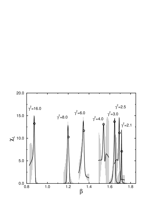
FIG. 12.: $\beta$ dependence of the Polyakov loop susceptibility obtained by the histogram method on an $8^{4}\times 4$ lattice with $\gamma^{2}\geq 2.1$. The circles denote the simulation point.

FIG. 13.: $\beta$ dependence of the Polyakov loop susceptibility obtained by the histogram method on an $8^{4}\times 6$ lattice with $\gamma^{2}\geq 4.0$. The circles denote the simulation point.

FIG. 14.: Large peaks of the Polyakov loop susceptibility obtained by the histogram method at $\gamma^{2}=2.0$ on an $8^{4}\times 4$ lattice, and $\gamma^{2}=3.6$ and $3.8$ on an $8^{4}\times 6$ lattice, respectively.

FIG. 15.: Flip-flop in the history of the plaquette value at $\gamma^{2}=4.0$ on an $8^{4}\times 4$ lattice.

FIG. 16.: Phase transition points for $N_{5}=4$ $(\circ)$ and $N_{5}=6$ $(\Diamond)$ in the $\beta-\gamma$ plane. Two solid lines denote the boundaries of the region in which two kind of phases coexist. Compare the figure with Fig. 10.

FIG. 17.: $\bar{\beta}_{\rm lat}$ as a function of $s$ determined on the transition lines of $N_{5}=4$ $(\circ)$ and $N_{5}=6$ $(\Box)$. The figures shows the physical equivalence between the critical lattice systems.

FIG. 18.: The power-law behavior of $g^{-2}$ as a function of $s$ determined on the transition lines of $N_{5}=4$ $(\circ)$ and $N_{5}=6$ $(\Box)$, where the straight line is the one-loop line (40).

FIG. 19.: Scaling behavior of the Creutz ratio along the $\gamma^{2}=4.0$ line on an $8^{4}\times 4$ lattice. The solid line is $\ln(\chi)=2\ln|\beta-D_{2}|+1.2$ (see Eq.(63)), where $D_{2}=2.156(23)$.

FIG. 20.: Scaling behavior of the Creutz ratio for $N_{5}=2,3,4,5,6$ and $8$ measured on the line expected from the one-loop $\beta$-function (40). The open symbols are the results of the ordered start and the filled symbols are those of the disordered start.