Event-by-event fluctuations of the charged particle ratio from non-equilibrium transport theory

Abstract

The event by event fluctuations of the ratio of positively to negatively charged hadrons are predicted within the UrQMD model. Corrections for finite acceptance and finite net charge are derived. These corrections are relevant to compare experimental data and transport model results to previous predictions. The calculated fluctuations at RHIC and SPS energies are shown to be compatible with a hadron gas. Thus, deviating by a factor of 3 from the predictions for a thermalized quark-gluon plasma.

In this note we exploit a novel idea of a signal proposed by [1] based on event by event fluctuations of the $N_{+}/N_{-}$ ratio ($N_{+}$ and $N_{-}$ being positively and negatively charged hadrons). In particular, we would like to precisely specify the observable which is to be compared with the prediction of Ref.[1]. The magnitude of these fluctuations was estimated from thermodynamics to be a factor of 3 different for a QGP compared to a conventional hadronic gas. The predictions of [1] were derived using a grand canonical ensemble and assuming a zero net charge. In a grand canonical ensemble charge is conserved only on the average, whereas charge is conserved event-by-event in real heavy ion collisions and the model calculations presented here. The assumption of a grand canonical ensemble thus is only valid in the limit of $P\equiv{\langle N_{\rm ch}\rangle}_{\Delta y}/{\langle N_{\rm ch}\rangle}_{\rm total}\rightarrow 0$ and correction to that are of the type $(1-P)$ [1, 2]. Thus, in order to compare experimental data with the predictions of [1], corrections have to be applied, which will be presented here.

For our study of this observable, we employ the Ultra-relativistic Quantum Molecular Dynamics model (UrQMD) [3]. This model has been shown to reproduce the measured data on event-by-event fluctuations in Pb+Pb collisions at the SPS [4]. UrQMD is a microscopic transport approach based on the covariant propagation of constituent quarks and diquarks accompanied by mesonic and baryonic degrees of freedom. It simulates multiple interactions of ingoing and newly produced particles, the excitation and fragmentation of color strings and the formation and decay of hadronic resonances. At SPS and RHIC energies, the treatment of subhadronic degrees of freedom is of major importance. In the UrQMD model, these degrees of freedom enter via the introduction of a formation time for hadrons produced in the fragmentation of strings [5]. The leading hadrons of the fragmenting strings contain the valence-quarks of the original excited hadron. In UrQMD they are allowed to interact even during their formation time, with a reduced cross section defined by the additive quark model, thus accounting for the original valence quarks contained in that hadron [3]. The thermodynamics properties of the model in equilibrium are similar to a Hagedorn gas with a limiting temperature of 135 MeV [6].

Let us shortly review the main ideas of the charge fluctuations as elaborated in [1]. The following connection between the observable charge ratio fluctuations and the fluctuations of the elementary net charges of the system has been proposed:

$$D=\langle N_{\rm ch}\rangle\langle\delta R^{2}\rangle\approx 4\langle\delta Q^{2}\rangle/\langle N_{\rm ch}\rangle\quad,$$ (1)

with $Q=\sum_{a}q_{a}N_{a}$, where $a$ runs over all hadron/parton species in the interval $\Delta y\ll y_{\rm total}$ in an event and $q_{a}$ is the charge of the species $a$ and $N_{a}$ is the number of particles of species $a$. The ratio fluctuations $\langle\delta R^{2}\rangle$ are defined by

$$\langle\delta R^{2}\rangle=\langle R^{2}\rangle-\langle R\rangle^{2}\quad,$$ (2)

where the $\langle\dots\rangle$ denotes event averaging. The ratio $R=N^{+}/N^{-}$ is obtained for each event separately in the given rapidity interval $\Delta y$ by counting the charges of the hadrons. Note that weak decays are not taken into account - in line with the experimental setups.

As already mentioned at the beginning of this letter, the predictions for $D$ obtained in [1] are based on a grand canonical ensemble assuming zero net charge in the system. In reality, the system under consideration has a small but finite net charge. Also, the assumption of a grand canonical ensemble is only justified in the limit of $P\rightarrow 0$.

For a finite acceptance, transport model calculations and the experimental data need to be corrected in order to be compared with the predictions of [1] (see Eq. 15). One observation is that as $P\to 1$, the charge fluctuation has to vanish because the global charge does not fluctuate. Also Eq.(1) is no longer valid in the same limit if the net charge of the system under consideration is non-zero.

The complete analysis is fully explained in the upcoming paper [7]. In this letter, we list the key results. In terms of $N_{+}$ and $N_{-}$, the ratio fluctuation is given by [8]

$${\langle\delta R^{2}\rangle}_{\Delta y}=\tilde{R}_{\Delta y}^{2}\,\left\langle\left({\delta N_{+}\over{\langle N_{+}\rangle}_{\Delta y}}-{\delta N_{-}\over{\langle N_{-}\rangle}_{\Delta y}}\right)^{2}\right\rangle_{\rm\Delta y}$$ (3)

where ${\langle\dots\rangle}_{\Delta y}$ is the event average in a given rapidity window $\Delta y$ and

$$\tilde{R}_{\Delta y}\equiv{\langle N_{+}\rangle}_{\Delta y}/{\langle N_{-}\rangle}_{\Delta y}\;.$$ (4)

In an ideal detector with full coverage, the ratio fluctuation is

$${\langle\delta R^{2}\rangle}_{\rm total} = w_{H}\,\tilde{R}_{\rm total}^{2}\,{Z_{0}^{2}\over{\langle N_{-}\rangle}_{\rm total}\,{\langle N_{+}\rangle}_{\rm total}^{2}}$$ (5)

where $Z_{0}$ is the fixed total charge in the system, $w_{H}={\langle\delta N_{-}^{2}\rangle}/{\langle N_{-}\rangle}\approx 1$, Here ${\langle\dots\rangle}_{\rm total}$ denotes the event average in the full phase space. At SPS, ${\langle\delta R^{2}\rangle}_{\rm total}\sim 1\%$ and at RHIC, ${\langle\delta R^{2}\rangle}_{\rm total}\sim 10^{-5}$. This is a consequence of the charge conservation. No detailed information on dynamics can be obtained from Eq.(5).

Having a finite rapidity window modifies the above full phase space result in an essential way. The particle number in a given rapidity bin now has two independent source of fluctuations:

• Event-by-event fluctuation in the overall number $N_{r}$ of a given particle species $r$ due to different impact parameters and inelasticities.

• Given a class of events with the same $N_{r}$, additional fluctuations in a specific rapidity window occur due to different distributions of the $N_{r}$ particles in phase space.

These two fluctuations are independent of each other. The squares of the fluctuations are additive. Note that the grand canonical ensemble approach requires $\Delta y\ll y_{\rm total}$, therefore the fluctuations from (i) are negligible as shown below.

Assuming that the fluctuations (ii) follow a binomial distribution and that the probability $P$ is the same for all species of particles, the number fluctuations in a given rapidity window are

$${\langle\delta N^{2}\rangle}_{\Delta y} = P^{2}{\langle\delta N^{2}\rangle}_{\rm total}+P(1-P){\langle N\rangle}_{\rm total}$$ (6)

$$= P^{2}{\langle\delta N^{2}\rangle}_{\rm total}+(1-P){\langle N\rangle}_{\Delta y}\;,$$ (7)

where ${\langle\dots\rangle}_{\Delta y}$ denotes the event average within $\Delta y$ and we used ${\langle N_{\rm ch}\rangle}_{\Delta y}=P{\langle N_{\rm ch}\rangle}_{\rm total}$.

In the ratio ${\langle\delta N^{2}\rangle}_{\Delta y}/{\langle N_{\pm}\rangle}_{\Delta y}^{2}$ needed to construct ${\langle\delta R^{2}\rangle}_{\Delta y}$ (c.f. Eq.(3)), the $P^{2}$ factor in the first term cancels. (The same holds for the cross terms.) Hence, the contribution of the first term is ${\langle\delta R^{2}\rangle}_{\rm total}$ in Eq.(5). The second term replaces ${\langle R\rangle}$ factor in Eq.(10) in Ref.[8] to yield

$${\langle\delta R^{2}\rangle}_{\Delta y} = {\langle\delta R^{2}\rangle}_{\rm total}\left({\tilde{R}_{\Delta y}^{2}\over\tilde{R}_{\rm total}^{2}}\right)+(1-P)\tilde{R}_{\Delta y}^{2}D_{+-}^{2}\;,$$ (8)

where $D_{+-}^{2}$ is the expression given in Eq.(13) in Ref.[8].

The prediction given in Ref.[1] is for ${\langle N_{\rm ch}\rangle}_{\Delta y}D_{+-}^{2}$. To extract $D_{+-}^{2}$ from Eq.(8), we need to apply two correction factors, $C_{\mu}=\tilde{R}_{\Delta y}^{2}$ and $C_{y}=(1-P)$. Thus, collecting the correction factors yields

$${{\langle N_{\rm ch}\rangle}_{\Delta y}{\langle\delta R^{2}\rangle}_{\Delta y}\over C_{\mu}C_{y}}={\langle N_{\rm ch}\rangle}_{\Delta y}D_{+-}^{2}+{P\over(1-P)}\left({\langle N_{\rm ch}\rangle}_{\rm total}{{\langle\delta R^{2}\rangle}_{\rm total}\over\tilde{R}_{\rm total}^{2}}\right)\approx{\langle N_{\rm ch}\rangle}_{\Delta y}D_{+-}^{2}\;,$$ (9)

where ${\langle N_{\rm ch}\rangle}_{\Delta y}=P{\langle N_{\rm ch}\rangle}_{\rm total}$ is used. For $P<1$, the second term is negligible at SPS and at RHIC.

Let us summarize the correction factors that need to be applied to take care of the effects of the finite net charge and the finite acceptance window.

1. In order to correct for the finite net charge within the acceptance due to baryon stopping, one has to apply a factor $C_{\mu}$ given by

   $$C_{\mu}=\tilde{R}^{2}_{\Delta y}={{\langle N_{+}\rangle}^{2}_{\Delta y}\over{\langle N_{-}\rangle}^{2}_{\Delta y}}$$ (10)

   to the experimental data and the model calculations to compare with the pion gas and quark gas result of [1].

2. In order to correct for the finite bin size in rapidity, and in order to incorporate global charge conservation one has to rescale the experimental data and the transport model predictions by a factor of

   $$C_{y}=1-P=1-\frac{\langle N_{\rm ch}\rangle_{\Delta y}}{\langle N_{\rm ch}\rangle_{\rm total}}\quad.$$ (11)

Thus, the basic observable to be compared with the predictions calculated in [1] is

$$\tilde{D}={{\langle N_{\rm ch}\rangle}_{\Delta y}{\langle\delta R^{2}\rangle}_{\Delta y}\over C_{\mu}\,C_{y}}=\left\{\begin{array}[]{ll}1&\hbox{quark gluon gas}\\ 2.8&\hbox{resonance gas}\\ 4&\hbox{uncorrelated pion gas}\end{array}\right.$$ (15)

Again the subscript $\Delta y$ denotes the average taken in the rapidity acceptance, while the subscript ‘total’ indicates the average of $4\pi$ acceptance.

Fig. 1 shows the $\tilde{D}$ values as predicted by the UrQMD model (symbols) as compared to the estimates for the resonance gas (dashed line) and the quark gluon gas (full line). The shown acceptance cuts are chosen according to the experimentally accessible rapidity windows of the NA49 ($2.5\leq y\leq 4.5$) and STAR ($-1\leq y\leq 1$) detectors. One observes, that the UrQMD model predictions of the charge ratio fluctuations are in agreement with the expectations of a hadron gas. The predicted fluctuations are a factor of 3 larger than the fluctuations expected if a QGP was formed. Thus, the proposed observable – the charge ratio fluctuations – predicted for a QGP can not be mimicked by either multiple string break-up nor strong rescattering effects which may drive the system towards an equilibrated Hagedorn gas behavior.

Fig. 2 explores the fluctuation parameter $\tilde{D}$ as a function of the width of the inspected rapidity window ($y_{\rm cm}\pm\frac{\Delta y}{2}$) in Au+Au, $b\leq 2$ fm at $\sqrt{s}=200$ AGeV. Full squares denote the charge ratio fluctuation values obtained with all corrections included as discussed above. Open squares show the charge ratio fluctuation values without the correction for finite rapidity window and net charge. In line with the findings of [9], one observes a strong decrease in the fluctuation values if no correction is applied. However, the inclusion of the necessary corrections (see Eqs. 10 and 11) yields fluctuations similar to the ones obtained from a resonance gas over all inspected rapidities. Notice further the increase of the values obtained from UrQMD in rapidity windows of $\Delta y\leq 2$. This increase is due to the vanishing correlations from resonance decays which is present at larger rapidity windows. Details are discussed in [8] (see also [2]).

In conclusion, the charge ratio fluctuations at SPS and RHIC energies are predicted from the UrQMD model and compared to a hadron gas and QGP estimate. It is shown that the UrQMD model results are compatible with the formation of a hadron gas at SPS and RHIC energies. The transport model simulations predict fluctuations that are by a factor of 3 larger then the fluctuations characteristic for QGP formation. The dependence of the fluctuation on the rapidity width is predicted and shown to be compatible with a resonance gas if all corrections are included. This observable can be easily studied as ‘Year 1’ observable with STAR at RHIC. It can also be directly accessed by the NA49 experiment at the CERN-SPS.

Finally let us stress that it is the corrected observable $\tilde{D}$ defined in Eq. (15) that must be compared with our predictions. A measurement of $\tilde{D}\simeq 1$ indicates the presence of a QGP state in the system created by the heavy ion collision.

FIG. 1.: The corrected fluctuation parameter $\tilde{D}=\langle N_{\rm ch}\rangle_{\Delta y}\langle\delta R^{2}\rangle_{\Delta y}/(C_{\mu}C_{y})$ as a function of centrality. Circles denote Pb+Pb collisions at 160AGeV, while squares denote Au+Au collision at $\sqrt{s}=200$ AGeV as predicted by the UrQMD model. The dashed line show the analytical predictions for a hadron gas [1], while the full line depicts the value obtained from lattice QCD [1].

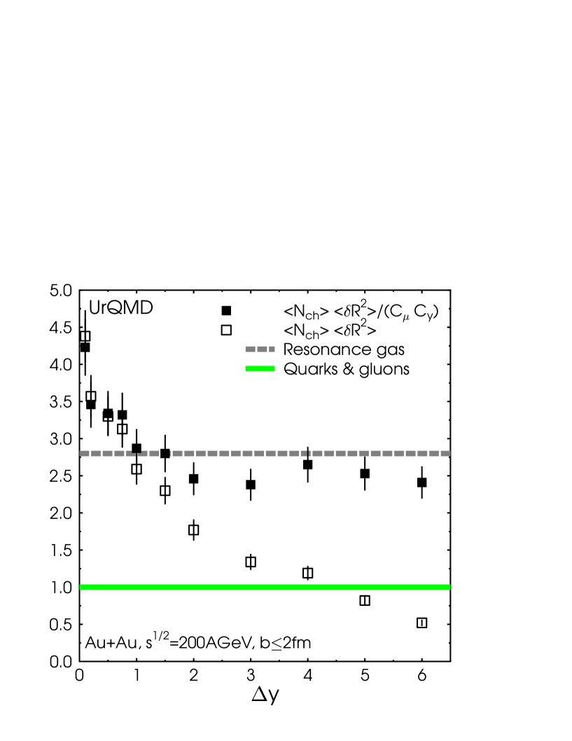
FIG. 2.: Fluctuation parameter $\tilde{D}=\langle N_{\rm ch}\rangle_{\Delta y}\langle\delta R^{2}\rangle_{\Delta y}/(C_{\mu}C_{y})$ and $D=\langle N_{\rm ch}\rangle_{\Delta y}\langle\delta R^{2}\rangle_{\Delta y}$ as a function of the width of the rapidity window ($y_{\rm cm}\pm\frac{\Delta y}{2}$) in Au+Au, $b\leq 2$ fm at $\sqrt{s}=200$ AGeV as predicted by the UrQMD model. Full squares denote the charge fluctuation values $\tilde{D}$ obtained with all corrections included. Open squares show the charge fluctuation values $D$ without the correction for finite rapidity window and net charge. The lines are the same as in Fig. 1.

REFERENCES

- [1] S. Jeon and V. Koch, hep-ph/0003168.
- [2] H. Heiselberg and A. Jackson, nucl-th/0006021.
-
[3]
S. A. Bass et al., Prog. Part. Nucl. Phys. 41, 225 (1998);
M. Bleicher et al, J. Phys. G 25 (1999) 1895 - [4] M. Bleicher et al., Phys. Lett. B435, 9 (1998) [hep-ph/9803345].
-
[5]
B. Andersson, G. Gustavson, and B. Nilsson-Almquist,
Nucl. Phys. B281, 289 (1987);
B. Andersson et al., Comp. Phys. Comm. 43, 387 (1987);
T. Sjoestrand, Comp. Phys. Comm. 82, 74 (1994). - [6] M. Belkacem et al., Phys. Rev. C58, 1727 (1998) [nucl-th/9804058].
- [7] M. Bleicher, S. Jeon and V. Koch, in preparation.
- [8] S. Jeon and V. Koch, Phys. Rev. Lett. 83, 5435 (1999) [nucl-th/9906074].
- [9] K. Fialkowski and R. Wit, hep-ph/0006023.