Velocity distributions and annual-modulation signatures of weakly-interacting massive particles

Abstract:

An annual modulation in the event rate of the NaI detector of the Dama collaboration has been used to infer the existence of particle dark matter in the Galactic halo. Bounds on the WIMP mass and WIMP-nucleon cross section have been derived. These analyses have assumed that the local dark-matter velocity distribution is either isotropic or has some bulk rotation. Here we consider the effects of possible structure in the WIMP velocity distribution on the annual-modulation amplitude. We show that if we allow for a locally anisotropic velocity dispersion tensor, the interpretation of direct detection experiments could be altered significantly. We also show that uncertainties in the velocity distribution function that arise from uncertainties in the radial density profile are less important if the velocity dispersion is assumed to be isotropic.

1 Introduction

Weakly interacting massive particles (WIMPs) are among the leading candidates for dark matter in galactic halos. Such particles arise naturally in extensions to the standard model (SM) of particle physics; an example is the neutralino, plausibly the lightest superpartner in supersymmetric versions of the SM. Massive particles whose coupling with lighter SM particles have interactions of electroweak strength have a cosmological abundance of order the critical density of the Universe. Hence, WIMPs appear naturally as dark-matter candidates. The possibility to link these two apparently separate problems (electroweak symmetry breaking and dark matter) was realized a couple of decades ago, and since then the search for WIMPs in the Milky Way halo has been a major endeavor both theoretically and experimentally (for a comprehensive review see Ref. [1]).

Numerous complementary techniques have been developed in order to detect relic WIMPs. Currently, the most promising method is probably direct detection through observation, in a low-background laboratory detector, of nuclear recoils due to WIMP-nucleus elastic scattering [2, 3]. The chance for a given WIMP to interact in the detector is very low and the energy released in case of interaction is expected to be tiny (in the keV range). Nevertheless, this detection method has already had a few successes. It has been exploited to exclude as the main component of the dark Galactic halo WIMP candidates such as a fourth-generation heavy neutrino and the sneutrino [4]. Detectors have now reached the sensitivity to start probing the region of parameter space of interest if a neutralino is the dark matter (see e.g. Ref. [5]). Recently, the Dama [6] and Cdms [7] collaborations, while probing roughly the same region of parameter space, have presented apparently contradictory results, a possible WIMP signal in the first case and a null result in the second. It is probably premature to derive any conclusion from these results, but, with further data and even more sensitive detectors being developed, the next years promise to be very exciting for the field.

To claim a positive detection, an experiment must be able to discriminate the signal from backgrounds. In principle, the shape of the recoil spectrum can be used, since the recoil spectra from WIMPs and background should generally differ. However, the shape of the recoil-energy spectrum for WIMP-nucleus scattering cannot be predicted with enough precision to separate it from the background, the spectrum of which is generally not understood in detail. A possible way out is to look for a slight annual modulation in the event rate (see Refs. [3, 8]; among more recent works see, e.g., Refs. [9, 10]). Such an effect is expected for the WIMP signal, but not for the background. This is the signature exploited in the data analysis by the Dama collaboration to claim detection of WIMPs. The underlying idea is quite simple. Like all other stars in the rotationally-supported disk, the Sun is moving around the Galactic center on a roughly circular orbit, passing through the dark halo which is believed on the other hand to be static and not rotationally supported. The Earth, and detectors on it, contain this velocity component plus an additional component due to the orbital motion around the Sun. The azimuthal velocity of the Sun and the projection of the velocity of the Earth on the galactic plane are most closely aligned near June 2 and most anti-aligned six months later. The WIMP-nucleus interaction rate in a detector depends on the velocities of the incident WIMPs. Hence, a yearly modulation of the signal is expected.

In prior analyses of the modulation effect, the local dark-matter velocity distribution was assumed to be a Maxwell-Boltzmann distribution (which is, of course, isotropic), as would arise if the Galactic halo is isothermal. Velocity distributions for halos with some bulk rotation have also been considered [10]. Although these velocity distributions are consistent with current data on the Milky Way, there are other plausible, consistent, and possibly even better-motivated alternatives. For example, results from N-body simulations of hierarchical clustering favor density profiles which are steeper at large galactocentric distances than the $r^{-2}$ decline in the isothermal sphere and which are cuspy in the Galactic center, rather than cored, and the velocity distribution corresponding to a cuspy halo should differ from the Maxwell-Boltzmann distribution that corresponds to an isothermal halo.

Moreover, it is plausible that the velocity distribution may be anisotropic rather than isotropic as usually assumed. In fact, most of the visible populations in the Galactic halo show some degree of anisotropy (e.g., the stars in the local neighborhood and globular clusters). Furthermore, the inefficiency of phase mixing that results in a cuspy profile (rather than an isothermal sphere) should leave some degree of anisotropy in the velocity-dispersion tensor. Some evidence for a global preference for predominantly radial velocities is already seen in the simulations [11], as well as in globular clusters [12]. Even if the global velocity distribution is isotropic, clumping in velocity space, which may also arise if phase mixing is not perfectly efficient during gravitational collapse, may yield a locally anisotropic velocity dispersion.

Prior work has shown that the direct-detection rate should not depend sensitively on the details of the velocity distribution [13]. However, this work considered only the total detection rate, integrated over all nuclear-recoil energies. The modulation signal in Dama depends on details of the differential energy distribution. The purpose of this paper will be to show that the amplitude of the modulation can thus depend quite sensitively on the precise form of the velocity distribution. The inferred WIMP cross sections and masses could thus be altered.

The outline of the paper is the following. In the next Section we discuss a procedure to relate the velocity distribution to the Galactic density distribution. In Section 3 we review WIMP direct detection rates and the annual modulation effect. The main results are given in Section 4. In Section 5 we summarize and make some concluding remarks.

2 Dark-matter distribution functions

We suppose that the dark-matter halo of the Milky Way is roughly spherical, and among the general family of profiles,

$$\rho_{\rm{dm}}(r)=\rho_{0}\left(\frac{R_{0}}{r}\right)^{\gamma}\left[\frac{1+(R_{0}/a)^{\alpha}}{1+(r/a)^{\alpha}}\right]^{(\beta-\gamma)/\alpha},$$ (1)

we focus on functional forms suggested by N-body simulations (in the equation above $\rho_{0}$ and $R_{0}$ are respectively the local dark-matter density and the Sun galactocentric distance). We restrict ourselves mainly to the Navarro, Frenk, and White profile [14], which has $(\alpha,\beta,\gamma)=(1,3,1)$ (hereafter the NFW profile). We will show also that the behavior of the profile towards the Galactic center is not critical in our analysis by considering the more cuspy Moore et al. profile [15], $(\alpha,\beta,\gamma)=(1.5,3,1.5)$, and the less singular profile of Kravtsov et al. [16], $(\alpha,\beta,\gamma)=(2,3,0.4)$. The value of the scale radius $a$ which appears in Eq. (1) is determined in the N-body simulations as well, depending on the mass of the simulated halo. We infer its approximate value for the NFW and Moore et al. profiles in case of an $\Omega_{M}=0.3$ cosmology from Refs. [15, 17]. The approach we follow to fix the remaining unknown parameters, both in the dark-halo profile and in the functions that describe the luminous components of the Milky Way, is to perform a combined best fit of available observational data, taking into account the kinematics of local stars, the rotation curve of the Galaxy, the dynamics of the satellites, and more (details are given in Ref. [18]). Sample values for the subset of parameters relevant in the present analysis are specified in Table 1 (mass decompositions for the Milky Way are highly degenerate, so slightly different values are compatible as well). Thus, we have a family of spherically-symmetric radial profiles that are all theoretically plausible and consistent with all known observational constraints.

Parameter	$\rho_{0}$	$a$	$M_{b}$	$M_{d}$
Units	GeV cm-3	kpc	1010 M⊙	1010 M⊙
NFW	0.3	20	0.8	5.1
Moore et al.	0.3	28	1.1	4.7
Kravtsov et al.	0.6	10	1.3	3.6

Table 1: Best-fit values for some relevant parameters in a few mass decompositions for the Milky Way. The three dark-matter-halo profiles considered are specified in the text. $M_{b}$ and $M_{d}$ are respectively the total mass of the bulge and of the disk (stars + gas). We assumed that the Sun galactocentric distance is 8 kpc.

We will now find the velocity distributions that correspond to these halo profiles. The density distribution does not determine the velocity distribution uniquely. To sample the possibilities, we will therefore first find velocity distributions that have isotropic velocity distributions, and then find some distributions that have preferentially radial velocities.

If we assume an isotropic velocity distribution, then there is a one-to-one correspondence between the spherically symmetric density profile $\rho(r)$ and its distribution function given by Eddington’s formula [19],

$$F({\cal E})=\frac{1}{\sqrt{8}\pi^{2}}\left[\int_{0}^{{\cal E}}\frac{d^{2}\rho}{d\Psi^{2}}\frac{d\Psi}{\sqrt{{\cal E}-\Psi}}+\frac{1}{\sqrt{{\cal E}}}\left(\frac{d\rho}{d\Psi}\right)_{\Psi=0}\right]$$ (2)

where $\Psi(r)=-\Phi(r)+\Phi(r=\infty)$, with $\Phi$ the potential of the system, ${\cal E}=-E+\Phi(r=\infty)=-E_{\rm{kin}}+\Psi(r)$, and $E$ and $E_{\rm{kin}}$, respectively, the total and kinetic energy. Eq. (2) works for a single isolated self-gravitating system. However, the Milky Way has a complex structure containing a bulge elongated into a bar, a flattened disk, and maybe a triaxial dark halo. For the present purpose, however, it is sufficient to consider a toy model in which all components are assumed to be spherical. Even the awkward approximation of a “spherical” disk will have little influence on our conclusions. In such a toy model, we can alter Eq. (2) to provide the dark-matter distribution function by replacing $\Psi$ and $\rho$ (appropriate for an isolated system) by $\Psi_{\rm{tot}}$ and $\rho_{\rm{dm}}$, respectively, the gravitational potential due to all components and the dark matter density profile. Actually, it is easier from the numerical point of view to implement Eq. (2) by changing the integration variable from $\Psi_{\rm{tot}}$ to the radius of the spherical system $r$. Then Eq. (2), in case of the dark-matter halo distribution function, becomes,

$$F_{\rm{dm}}({\cal E}) = \frac{1}{\sqrt{8}\pi^{2}}\int_{\Psi_{\rm{tot}}^{-1}({\cal E})}^{\infty}\frac{dr}{\sqrt{{\cal E}-\Psi_{\rm{tot}}(r)}}\left[\frac{d\rho_{\rm{dm}}}{dr}\frac{d^{2}\Psi_{\rm{tot}}}{dr^{2}}\left(\frac{d\Psi_{\rm{tot}}}{dr}\right)^{-2}\right.$$ (3)

$$\left.-\frac{d^{2}\rho_{\rm{dm}}}{dr^{2}}\left(\frac{d\Psi_{\rm{tot}}}{dr}\right)^{-1}\right]\;.$$

If we relax the hypothesis of isotropy of the velocity dispersion tensor, the most general distribution function corresponding to a spherical density profile is a function of ${\cal E}$ and $L$, the magnitude of the angular-momentum vector. In such systems the velocity dispersion in the radial direction is different from that in the azimuthal direction (which is equal to the one in the other tangential direction) [19]. For a given radial density profile, the distribution function is not unique. We investigate a special class of models, the Osipkov-Merritt models [20, 21], in which $F$ is a function of ${\cal E}$ and $L$ only through the variable $\cal Q$:

$${\cal Q}\equiv{\cal E}-\frac{L^{2}}{2r_{a}^{2}}\;.$$ (4)

Here $r_{a}$ is called the anisotropy radius, as in the Osipkov-Merritt models the anisotropy parameter is [21]:

$$\beta(r)\equiv 1-\frac{\overline{v_{\phi}^{2}}}{\overline{v_{r}^{2}}}=\frac{r^{2}}{r^{2}+r_{a}^{2}}\;.$$ (5)

Therefore, $r_{a}$ is the radius within which the dispersion velocity is nearly isotropic. As already mentioned, in analogy with other observed populations, we will entertain the possibility that for the dark-matter halo $\overline{v_{r}^{2}}>\overline{v_{\phi}^{2}}$ and thus that $\beta>0$. The distribution function for this class of models is again easy to derive. It is sufficient to replace in Eq. (3) ${\cal E}$ with $\cal Q$ and $\rho_{\rm{dm}}(r)$ with $\rho_{\rm{dm}}^{\cal Q}(r)=(1+r^{2}/r_{a}^{2})\,\rho_{\rm{dm}}(r)$.

3 Direct-detection rates and annual-modulation effect

The differential direct-detection rate for dark-matter WIMPs in a given material (per unit detector mass) is [1],

$$\frac{dR}{dQ}=\frac{\rho_{0}}{M_{\chi}}\int_{|\vec{v^{\prime}}|\geq v_{\rm{min}}}d^{3}\vec{v^{\prime}}\;f(\vec{v^{\prime}})\,|\vec{v^{\prime}}|\,\frac{d\sigma}{dQ}\;,$$ (6)

where $Q$ is the energy deposited in the detector and $d\sigma/dQ$ is the differential cross section for WIMP elastic scattering with the target nucleus. We assumed here that WIMPs of mass $M_{\chi}$ account for the local dark matter density $\rho_{0}$ and have a local distribution in velocity space (in the rest frame of the detector) $f=F_{\rm{dm}}(r=R_{0})/\rho_{0}$. The lower limit of integration $v_{\rm{min}}$ is the minimum velocity required for a WIMP to deposit the energy $Q$.

Assuming that scalar interactions dominate (as is probably the case for neutralino elastic scattering with Ge and NaI, the materials used respectively by the Cdms and Dama experiments) and that the couplings with protons and neutrons are roughly the same, Eq. (6) can be rewritten as,

$$\frac{dR}{dQ}=\left(\frac{\rho_{0}\,\sigma_{p}^{\rm{scalar}}}{2}\right)\left[A_{N}^{2}\frac{M_{N}}{{M_{\chi}}^{3}}\left(1+\frac{M_{\chi}}{M_{p}}\right)^{2}{\cal F}^{2}(Q)\right]\int_{|\vec{v^{\prime}}|\geq v_{\rm{min}}}d^{3}\vec{v^{\prime}}\;\frac{f(\vec{v^{\prime}})}{|\vec{v^{\prime}}|}\;,$$ (7)

where $\sigma_{p}^{\rm{scalar}}$ is the WIMP-proton cross section at zero momentum transfer, $A_{N}$ and $M_{N}$ are the detector nucleus atomic number and mass, while ${\cal F}(Q)$ is the nuclear form factor. In the equation above, the terms in the round bracket are energy and detector independent; we will not consider them in what follows. The terms in the square brackets depend on the nucleus chosen for the detector, as well as on the energy and WIMP mass. When considering annual modulation, they play a weighting effect for those detectors, like NaI, which are not monatomic (the generalization of Eq. (7) to this case is straightforward). The last term,

$$T(Q,M_{N},M_{\chi},t) = \int_{|\vec{v^{\prime}}|\geq v_{\rm{min}}}d^{3}\vec{v^{\prime}}\;\frac{f(\vec{v^{\prime}})}{|\vec{v^{\prime}}|}=\int_{v_{\rm{min}}}^{\infty}dv^{\prime}\;v^{\prime}\int d\Omega^{\prime}\;f(v^{\prime},\Omega^{\prime})$$ (8)

$$\equiv \int_{v_{\rm{min}}}^{\infty}dv^{\prime}\;g(v^{\prime})\;,$$

depends on $Q$, $M_{N}$, and $M_{\chi}$ through $v_{\rm{min}}=[(QM_{N})/(2M_{r}^{2})]^{1/2}$, where $M_{r}$ is the WIMP-nucleus reduced mass. It is time dependent and gives rise to the annual-modulation effect. This might not be clear at first sight, as we wrote implicitly the temporal dependence in the change of variables between the detector rest frame and the galactic frame. In polar coordinates, the change of variable to the detector frame (primed system in our notation) is simply: $v_{r}=v_{r}^{\prime}$, $v_{\theta}=v_{\theta}^{\prime}$, and $v_{\phi}=v_{\phi}^{\prime}+v_{\oplus}$. The azimuthal shift $v_{\oplus}$ varies during the year; in June it is roughly $v_{\oplus}=\Theta_{0}+v_{E}$, while in December it is $v_{\oplus}=\Theta_{0}-v_{E}$, where $v_{E}\simeq 15\,\rm{km}\,\rm{s}^{-1}$ is the projection of the earth orbital velocity on the galactic plane, while $\Theta_{0}$ is the galactic circular velocity at the Sun’s position. The latter is given in terms of Oort’s constants and the galactocentric distance by:

$$\Theta_{0}=(A-B)R_{0}=(27.2\pm 0.9)\,R_{0}\;\rm{km}\,\rm{s}^{-1}\,\rm{kpc}^{-1}\;,$$ (9)

where the numerical value of $A-B$ comes from the determination from Cepheid proper motions measured by the Hipparcos satellite [22].

The amplitude of the annual modulation (keeping track of whether the signal is greater in June or December) for a monatomic detector is then,

$${\cal{A}}(Q,M_{N},M_{\chi})=\frac{T(Q,M_{N},M_{\chi},{\rm June})-T(Q,M_{N},M_{\chi},{\rm December})}{T(Q,M_{N},M_{\chi},{\rm June})+T(Q,M_{N},M_{\chi},{\rm December})}\;.$$ (10)

As mentioned, the formula for NaI has instead a weighting factor for each of the two nuclei. For a given detector and distribution function the value of $\cal{A}$ follows. To compute $g$ as defined in Eq. (8) the appropriate choice of integration variable are, in the isotropic case,

$$g(v^{\prime}) = 2\pi\,v^{\prime}\int_{0}^{\pi}d\alpha\;\sin\alpha\,\frac{F_{\rm{dm}}({\cal E})}{\rho_{0}}$$

$${\cal E} = \Psi(R_{0})-\frac{1}{2}\left({v^{\prime}}^{2}+2\cos\alpha\,v^{\prime}v_{\oplus}+v_{\oplus}^{2}\right)\;,$$ (11)

while in the anisotropic case,

$$g(v^{\prime}) = 2\,v^{\prime}\int_{0}^{2\pi}d\psi\int_{0}^{\pi}d\eta\;\sin\eta\,\frac{F_{\rm{dm}}(\cal{Q})}{\rho_{0}}$$

$$\cal{Q} = \Psi(R_{0})-\frac{1}{2}\left({v^{\prime}}^{2}+2\sin\psi\,\sin\eta\,v^{\prime}v_{\oplus}+v_{\oplus}^{2}\right)$$ (12)

$$-\frac{R_{0}^{2}}{2r_{a}^{2}}\left({v^{\prime}}^{2}\,\sin^{2}\eta+2\sin\psi\,\sin\eta\,v^{\prime}v_{\oplus}+v_{\oplus}^{2}\right)\;.$$

4 Results

Figure 1: The integrand $g(v)$ for the direct-detection signal for December (D) and January (J) for an NFW profile (solid) and isothermal profile (dashed) both with an isotropic velocity distribution. The differential detection rate for a given recoil energy $Q$ and WIMP mass $M_{\chi}$ is given by the area under the curve to the right of the minimum velocity $v_{\rm{min}}$. This minimum velocity can be inferred in case of a germanium detector from the intersection of the dotted curves for a given $M_{\chi}$ and $Q$. The annual-modulation amplitude is proportional to the difference in the areas under the J and D curves for velocities larger than $v_{\rm{min}}$. The function $g(v)$ is the same for other nuclei, but the dotted curves for $v_{\rm{min}}$ are different. Figs. 3(a) and 4 show dotted curves to determine $v_{\rm{min}}$ for Na and I, respectively. A galactocentric distance $R_{0}=8$ kpc was used.

4.1 Isotropic Velocity Distributions

We first consider distribution functions with isotropic velocity dispersions. In Fig. 1 we plot with a solid line the function $g(v^{\prime})$ defined above in case of a NFW profile, assuming the galactocentric distance to be $R_{0}=8\;{\rm kpc}$ and $\Theta_{0}$ as derived from Eq. (9). There are two solid lines in the figure; the one which is higher at the peak refers to the function $g$ in December, while the second one is appropriate for June. As shown in the previous Section, the amplitude ${\cal{A}}$ of the annual modulation is proportional to the difference between June and December of the integral of $g$ above the value $v_{\rm{min}}$, which in turn depends on the energy deposited in the detector and WIMP and nucleus masses. As a visual aid to identify which are the relevant portions of the curves in each case, we plot in the figure the value of $v_{\rm{min}}$ for a Germanium detector and a few values of $Q$ and $M_{\chi}$ (e.g. $v_{\rm{min}}(Q=30\;{\rm keV},M_{\chi}=60\;{\rm GeV})$ is given by the abscissa of the point at the intersection between the horizontal dotted line labeled $Q=30\;{\rm keV}$ and the vertical dotted line labeled $M_{\chi}=60\;{\rm GeV}$). Analogous plots for Na and I are given in Figs. 3 and 4.

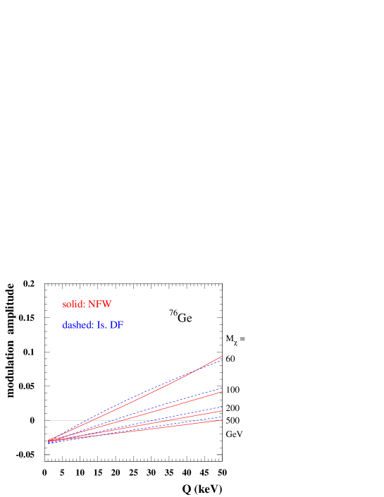
Figure 2: The annual-modulation amplitude for germanium as a function of nuclear-recoil energy $Q$ for $R_{0}=8$ kpc for the NFW (solid) and isothermal (dashed) profiles with isotropic velocity distributions for several WIMP masses $M_{\chi}$.

In Fig. 2 we plot the predicted annual-modulation amplitude as a function of $Q$, for this NFW profile, for a Germanium detector and for four sample values for the WIMP mass. As known from previous analyses, the modulation amplitude changes sign going to higher values of the deposited energy. At least for low-mass WIMPs, the largest values of ${\cal{A}}$ correspond to the largest displayed value of $Q$. Note however that at such large $Q$s the differential rate is almost negligible (being suppressed by the form factor ${\cal F}$).

To compare with the case previous analyses focussed on, we display in Fig. 1 the functions $g$ expected for an isothermal distribution function. The value for the velocity dispersion $\sigma$ is assumed accordingly to the naive (in the sense that it does not correspond to a self-consistent solution) prescription $\sigma=\sqrt{3/2}\;\Theta(R=\infty)$ and $\Theta(R=\infty)=\Theta_{0}$. We find a fairly good agreement with the NFW case and hence a consistency as well in the values of the modulation amplitude in Fig. 2.

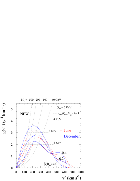
Figure 3: Like Fig. 1, but for anisotropic velocity distributions for the NFW radial profile. Here, the solid curve is for December and the dashed curve is for June, and curves are shown for several values ($\beta=0$, 0.2, and 0.4) of the anisotropy parameter. The dotted curves determine $v_{\rm{min}}$ for I.

We have checked that the effect we are trying to address does not depend sensitively on the steepness of the profile towards the Galactic center. The Moore et al. profile in Table 1 gives curves for $g$ barely distinguishable from the NFW curves in Fig. 1. This is because these two profiles have similar amounts of dark matter inside $R_{0}$ and analogous ratios of dark to luminous matter. The Kravtsov et al. profile in Table 1 has best-fit values for the local halo density $\rho_{0}$ and for length scale $a$ respectively higher and lower than in the previous cases; the dark matter happens then to be appreciably more concentrated toward the inner part of the Galaxy. In this case the velocity dispersion gets larger and hence values for the modulation amplitudes are reduced. We go in the direction of a slightly larger velocity dispersion also by dropping the hypothesis of having a “spherical disk”. We claim this in analogy to the isothermal case where it is relatively easy to construct a self-consistent solution for a thin disk and a flattened dark halo; this system has a velocity dispersion somewhat larger than in the purely spherical case.

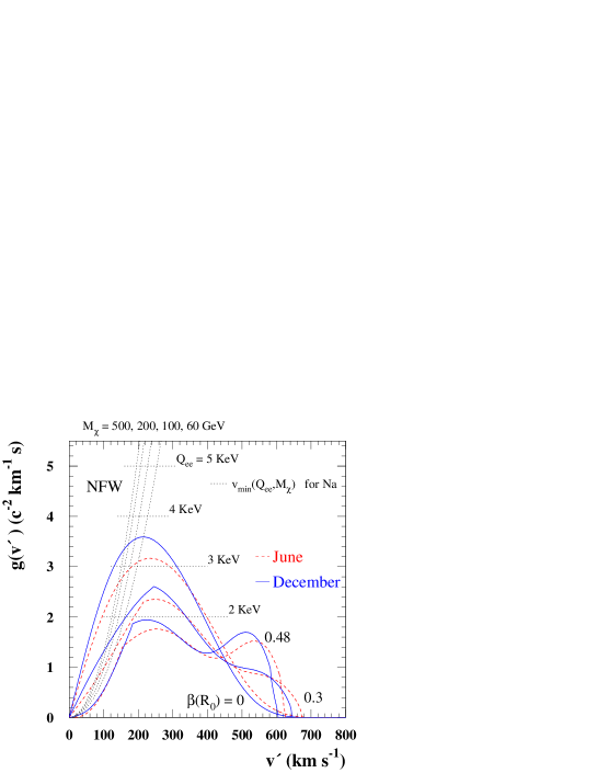
Figure 4: Like Fig. 3, but for values ($\beta=0$, 0.3, and 0.48) of the anisotropy parameter. Again, the solid curve is for December and the dashed curve is for June. The dotted curves determine $v_{\rm{min}}$ for Na.

4.2 Anisotropic Velocity Distributions

We sketch now what happens in case of anisotropy in the velocity dispersion tensor. As mentioned in Section 2, different approaches are possible; we consider the Osipkov-Merritt models applied to the NFW density profile introduced above. This will turn out to be sufficient to address the main qualitative effects. We suppose that the distribution function favors radial velocities. To illustrate the effects of anisotropy in the velocity distribution, we consider values for the anisotropy parameter $\beta(R_{0})$ in the range (0, 0.48). The upper value is close to the value of $\beta(R_{0})$ above which, with our particular choice of potential and dark-matter-density profile, the Osipkov-Merritt scheme breaks down.

In Fig. 3 we plot the forms for the function $g$ corresponding to $\beta(R_{0})=0.2$ and 0.4, as well as $\beta(R_{0})=0$. In Fig. 4 we plot instead the $\beta(R_{0})=0.3$ and 0.48 cases. It is evident that detector rest-frame values of the WIMP kinetic energy are, in anisotropic models, significantly redistributed (even though the spherically symmetric density profile remains unaltered). The enhancement at large $v^{\prime}$ is due to the fact that in these models there is a higher probability to have a contribution to the signal from particles on very elongated and nearly radial orbits (i.e. particles with $\cal{Q}$ close to zero; distribution functions analogous to the case considered here are given in Fig. 5 of Ref. [23]). Obviously this implies that the recoil energy spectra changes to some extent. However, without knowing the WIMP mass it may be hard, in case of a detection, to tell one spectrum induced by an anisotropic distribution from another due to an isotropic population for a different WIMP mass.

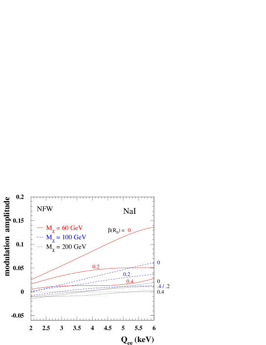
Figure 5: Like Fig. 2 but for Na instead of Ge and for the NFW profile with anisotropic velocity distributions with $\beta=0$, 0.2, and 0.4. Several different values of the neutralino mass are considered. Note also that here we plot $Q_{ee}$, the electron-equivalent energy that is measured by Dama, rather than the nuclear recoil energy. We see that the modulation amplitude may depend on the anisotropy of the velocity distribution, and the neutralino mass at which the modulation effect changes sign may also depend on the velocity anisotropy.

Regarding instead the annual-modulation signature, the effect can be quite dramatic. In Fig 5 we show the modulation amplitude for a NaI detector, plotting on the horizontal axis the electron equivalent energy $Q_{ee}$, rather than $Q$, in the range interesting for the Dama experiment (to derive this plot we assumed quenching factors and Woods-Saxon form factors as suggested by the Dama Collaboration [6]). As can be seen, for $\beta(R_{0})=0.4$, which corresponds to a local velocity ellipsoid for dark-matter particles that is still relatively close to spherical (the axis ratio is equal to 0.7), the modulation amplitudes in a NaI detector are severely damped. For intermediate neutralino masses and values of the recoil energy, the amplitude even changes sign. The $\beta(R_{0})=0.2$ case lies between the isotropic and 0.4 models. Still, the influence on the annual modulation is still rather large. Results for a Ge detector and in case of $\beta(R_{0})=0.48$ and 0.3 are shown in Fig 6 and are analogous to the NaI case.

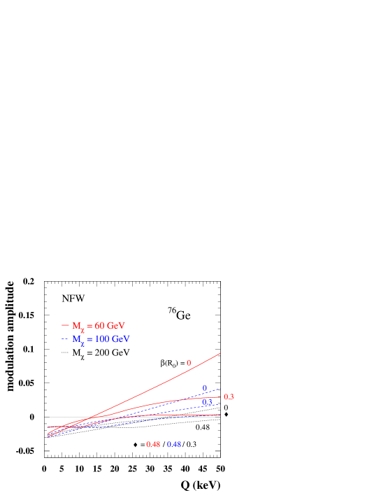
Figure 6: Like Fig. 4 but for Ge instead of Na. Here NFW profiles with anisotropic velocity distributions with $\beta=0$, 0.3, and 0.48 are considered.

5 Conclusions

We have investigated the possible effects on an annual-modulation signal of additional structure in the WIMP velocity distribution beyond the canonical Maxwell-Boltzmann distribution. To do so, we have considered isotropic distribution functions that correspond to density profiles other than the isothermal profile that goes with a Maxwell-Boltzmann velocity distribution, as well as some simple but plausible anisotropic velocity distribution functions.

The measured local rotation curve of the Milky Way fixes the velocity dispersion of any consistent dark-matter phase-space distribution. Thus, the total detection rate, integrated over all recoil energies, is expected to be independent of the detailed form of the velocity distribution. However, uncertainties in the velocity distribution can lead to larger uncertainties in the predicted detection rate if a signal is dominated primarily by events in a small recoil-energy bin, as occurs, for example, in the Dama annual-modulation signal. Moreover, the sign, as well as the magnitude, of the annual modulation can be changed. Thus, the constraints to the WIMP mass that are inferred from the sign of the modulation in Dama may be loosened if we allow for some structure in the phase-space distribution.

The anisotropic velocity distributions we used were chosen as they provide simple deviations from a Maxwell-Boltzmann distribution that illustrate our point. There are other possibilities for the phase-space distribution that are more complicated, although perhaps better motivated. For example, the existence of an NFW profile—rather than an isothermal profile—in numerical simulations suggests that phase mixing via violent relaxation is not fully efficient in gravitational collapse. If so, then some of the pre-collapse phase-space structure (recall that the pre-collapse phase-space structure of cold dark matter is very highly peaked around zero velocity) should be preserved. It is thus reasonable to expect some clumping in velocity space, even if the halo is smooth in physical space. Thus, for example, the local velocity distribution might be highly anisotropic even if the velocity distribution averaged over a larger volume of the Galaxy is isotropic. Although numerical simulations will be required to quantify this further, it is important to note the possible implications for WIMP-detection rates with the simple models we have considered.