QCD and the Structure of the Nucleon in Electron Scattering

Abstract

The internal structure of the nucleon is discussed within the context of QCD. Recent progress in understanding the distribution of flavor and spin in the nucleon is reviewed, and prospects for extending our knowledge of nucleon structure in electron scattering experiments at modern facilities such as Jefferson Lab are outlined.

1 Introduction

The internal structure of the nucleon is the most fundamental problem of strong interaction physics. Understanding this structure in terms of the elementary quark and gluon degrees of freedom of the underlying theory, quantum chromodynamics (QCD), remains the greatest unsolved problem of the Standard Model of nuclear and particle physics.

Historically, the basic strong interaction which we have sought to explain has been that between protons and neutrons in the atomic nucleus. The original idea of massive particle exchange of Yukawa [1] has been a guiding principle according to which later theories have been developed. It was pointed out by Wick [2] that this idea was consistent with the Heisenberg Uncertainty principle, whereby the interaction range of the nuclear force is inversely proportional to the mass of the exchanged meson. Over the years a phenomenological description of the forces acting between nucleons has been developed within a meson-exchange picture.

Following the experimental discovery of the pion in 1947, the 1950s and 1960s saw an explosion of newly discovered mesons and baryons, as particle accelerators pushed to higher energies. To bring some sense of order to the profusion of new particles, Gell-Mann and Zweig introduced the idea of quarks [3], which enabled much of the hadronic spectrum to be organized in terms of just a few elementary constituents. Soon after, however, it was realized that a serious problem existed with the simple quark classifications, namely the $\Delta^{++}$ isobar. The quark model wave function for the $\Delta^{++}$ was predicted to be totally symmetric, however the $\Delta^{++}$ obeyed Fermi-Dirac statistics. A solution to this problem was found by assigning extra internal color [4] quantum numbers to the quarks, in which baryons would have in addition an antisymmetric color wave function.

The discovery of scaling in deep-inelastic electron–nucleon scattering in the late 1960s at SLAC [5] confirmed that the nucleon contained point-like constituents, which were soon identified with the quarks of the quark model. Imposing local gauge invariance on the color fields, and introducing vector gluon exchange to mediate the inter-quark interaction, led naturally to the development of QCD as the fundamental theory of strong interactions [6].

Because QCD is an asymptotically free theory — the effective strong coupling constant decreases at short distances — processes involving large momentum transfers can be calculated reliably within perturbation theory. Yet despite the successes of perturbative QCD, we are still unable to extract from QCD sufficient details regarding its long-distance properties. This is because in the infra-red region the strong coupling constant grows and perturbation theory breaks down, and the available non-perturbative tools are not yet sufficiently developed to allow quantitative predictions.

In a sense it is ironic that the theory which arose out of the desire to understand nuclear forces is able to explain backgrounds in hadronic jets produced in high energy collisions, yet is unable to describe the properties of the ground state of the theory. Although one can argue that QCD in principle explains all hadronic and nuclear phenomena, without understanding the consequences of QCD for hadron phenomenology one may as well argue that the entire physics of atoms and molecules can in principle be explained from QED [7]. Understanding how the transition from the quarks and gluons of QCD to the physical mesons and baryons takes place remains the holy grail of modern nuclear physics.

In the next Section some basic elements of QCD relevant for later application to nucleon structure are reviewed. This is followed in Section 3 by the basic definitions and kinematics of electron–nucleon scattering, including elastic, deep-inelastic and semi-inclusive scattering. In Section 4 we focus more closely on the flavor and spin content of the nucleon, and outline some recent highlights in the study of valence and sea quark distributions. Finally, some concluding remarks are made in Section 5.

2 Elements of QCD

Quantum Chromodynamics is a non-Abelian gauge field theory based on the gauge group SU(3)_color, and defined in terms of the Lagrange density ^6,8-10:

$${\cal L}_{\rm QCD} = {\cal L}_{\rm inv}\ +\ {\cal L}_{\rm gauge}\ +\ {\cal L}_{\rm ghost}\ ,$$ (1)

where ${\cal L}_{\rm inv}$ is the classical Lagrangian, invariant under local gauge transformations of the SU(3)_color group:

$${\cal L}_{\rm inv} = \overline{\psi}_{i,f}(i\gamma^{\mu}D_{\mu}-m_{f})_{ij}\psi_{j,f}\ -\ {1\over 4}F_{\mu\nu}^{a}F^{\mu\nu\ a}\ .$$ (2)

The quark fields $\psi_{i,f}$ (for a particular quark flavor $f=u,d,s,\cdots$ , with mass $m_{f}$) are labeled by color indices $i,j=1,2,3$. The covariant derivative is $D_{\mu}=\partial_{\mu}-igT^{a}A_{\mu}^{a}$, where $g$ is the QCD coupling constant and $T^{a}$ are the generators of the SU(3) group, with $a=1,\cdots,8$. In terms of the gluon field $A_{\mu}^{a}$ the gluon field strength tensor is $F_{\mu\nu}^{a}=\partial_{\mu}A_{\nu}^{a}-\partial_{\nu}A_{\mu}^{a}+gf^{abc}A_{\mu}^{b}A_{\nu}^{c}$, with $f^{abc}$ the SU(3) structure constants. The major differences between QCD and quantum electrodynamics is the appearance, due to the non-Abelian structure of the theory, of gluon self-couplings in the $F\cdot F$ term. This gives rise to 3- and 4-point gluon interactions which make the theory highly non-linear, but also leads to the property of asymptotic freedom (Section 3.2).

Under local gauge rotations the quark fields transform (dropping color and flavor indices) according to:

$$\psi(x) \rightarrow \psi^{\prime}(x)\ =\ U(x)\ \psi(x)\ ,$$ (3)

where $U$ is an SU(3) unitary matrix:

$$U(x) = \exp\left(i\theta^{a}(x)T^{a}\right)\ ,$$ (4)

with $\theta^{a}(x)$ real. The gluon fields transform according to:

$$A_{\mu}(x) \rightarrow A^{\prime}_{\mu}(x)\ =\ U(x)A_{\mu}(x)U^{-1}(x)+{i\over g}\left(\partial_{\mu}U(x)\right)U^{-1}(x)\ .$$ (5)

One can easily show that ${\cal L}_{\rm inv}$ is then invariant under these transformations.

The gauge invariance of the classical Lagrangian introduces some difficulties when quantizing the gauge theory. This problem is avoided with the introduction of an addition term, ${\cal L}_{\rm gauge}$, which fixes a specific gauge. In the Lorentz (covariant) gauge, one has ${\cal L}_{\rm gauge}=-(1/2\alpha)(\partial^{\mu}A^{a}_{\mu})^{2}$, where $\alpha$ is an arbitrary gauge parameter. Of course observables cannot depend on the choice of $\alpha$, and some common choices are $\alpha=1$ (Feynman gauge) and $\alpha\rightarrow 0$ (Landau gauge). Other, non-covariant, gauge choices are the Coulomb gauge ($\partial_{i}A^{a}_{i}=0$), the axial gauge ($A^{a}_{3}=0$), and the temporal gauge ($A^{a}_{0}=0$).

The Faddeev-Popov ghost density, ${\cal L}_{\rm ghost}=(\partial_{\mu}\bar{\chi}^{a})(\delta^{ab}\partial_{\mu}-gf^{abc}A_{\mu}^{c})\chi^{c}$, where $\chi^{a}$ and $\bar{\chi}^{a}$ are scalar anti-commuting ghost fields, ensures that the gauge fixing does not spoil the unitarity of the $S$-matrix. Further discussion about the gauge fixing problem can be found in Refs. [10, 11].

In renormalizable field theories such as QCD the strength of the interaction depends on the energy scale. A property almost unique to QCD is that the renormalized coupling constant decreases with energy — known as asymptotic freedom. The running of the QCD coupling with energy allows one to compute cross sections for any quark–gluon process using a perturbative expansion if the coupling is small. Writing the full QCD Lagrangian as ${\cal L}_{\rm QCD}={\cal L}_{0}+{\cal L}_{\rm I}$, where

$${\cal L}_{0} = \overline{\psi}(i\gamma^{\mu}\partial_{\mu}-m)\psi-{1\over 4}(\partial_{\mu}A^{a}_{\nu}-\partial_{\nu}A^{a}_{\mu})(\partial^{\mu}A^{a\ \nu}-\partial^{\nu}A^{a\ \mu})$$ (6)

$$-{1\over 2\alpha}(\partial^{\mu}A^{a}_{\mu})^{2}+(\partial^{\mu}\bar{\chi}^{a})(\partial_{\mu}\chi^{a})\$$

is the free Lagrangian, and

$${\cal L}_{\rm I} = g\ \overline{\psi}\gamma^{\mu}T^{a}\psi A^{a}_{\mu}-{g\over 2}f^{abc}(\partial_{\mu}A^{a}_{\nu}-\partial_{\nu}A^{a}_{\mu})A^{b\mu}A^{c\nu}$$ (7)

$$-{g^{2}\over 4}f^{abe}f^{cde}A^{a}_{\mu}A^{b}_{\nu}A^{c\mu}A^{b\nu}-gf^{abc}(\partial^{\mu}\bar{\chi}^{a})\chi^{b}A^{c}_{\mu}$$

the interaction part, one can derive from ${\cal L}_{\rm I}$ a complete set of Feynman rules for computing any scattering amplitude involving quarks and gluons ^8-11.

Perturbative QCD has been enormously successful in calculating hard processes in high energy lepton-lepton, lepton-hadron and hadron-hadron scattering. However, even at high energies one can never avoid the fact that the physical states from which the quarks and gluons emerge to undergo the hard scattering are hadrons, so that one always encounters soft scales in any strongly interacting system. While operator product expansions usually allow one to factorize the short and long distance dynamics, understanding the complete physical process necessarily requires going beyond perturbation theory.

Over the years the problem of non-perturbative QCD has been tackled on several fronts. The most direct way is to solve the QCD equations of motion numerically on a discretized space-time lattice [12]. Recent advances in lattice gauge field theory and computing power has made quantitative comparison of full lattice QCD calculations with observables within reach.

Alternative methods of tackling non-perturbative QCD involve the building of soluble, low-energy QCD-inspired models, which incorporate some, but not all, of the elements of QCD. Phenomenological input is then used to constrain the model parameters, and identify circumstances where various approximations may be appropriate. These approaches often exploit specific symmetries of QCD, which for some observables may bring out the essential aspects of the physics independent of the approximations used elsewhere. A good example of this, which has had extensive applications in low energy physics, is chiral symmetry.

Consider the classical quark Lagrange density in Eq.(2) in the limit where the mass of the quarks is zero:

$${\cal L}^{q}_{\rm inv} = \overline{\psi}i\gamma^{\mu}D_{\mu}\psi\ =\ \overline{\psi}_{L}i\gamma^{\mu}D_{\mu}\psi_{L}\ +\ \overline{\psi}_{R}i\gamma^{\mu}D_{\mu}\psi_{R}\ ,$$ (8)

where $\psi_{L,R}=(1/2)(1\pm\gamma_{5})\psi$ are left- and right-handed projections of the Dirac fields. Under independent global left- and right-handed rotations ${\cal L}^{q}_{\rm inv}$ remains unchanged. For $N_{f}$ massless quarks, the classical QCD Lagrangian is then said to have a chiral SU$(N_{f})_{L}\otimes$ SU$(N_{f})_{R}$ symmetry. Of course non-zero quark masses break this symmetry explicitly by mixing left- and right-handed quark fields, however, for the $u$ and $d$ quarks, and to some extent the $s$, the masses are small enough for the chiral symmetry to be approximately valid.

If chiral symmetry were exact, a natural consequence would be parity doubling. The nucleon would have a negative parity partner with the same mass, and the pseudoscalar pion would have the same mass as the scalar meson. In nature, the lightest negative parity spin-1/2 baryon is the $S_{11}$ resonance, which is several hundred MeV heavier than the nucleon. Moreover, the pion has an exceptionally small mass, while the lightest candidate for a scalar meson is several times heavier than the pion, so that chiral symmetry in nature is clearly broken.

The way to reconcile a symmetry which is respected by the Lagrangian but broken by the physical ground state is if the symmetry is broken spontaneously. According to Goldstone’s theorem, a consequence of a spontaneously broken chiral symmetry is the appearance of massless pseudoscalar bosons. For $N_{f}=2$ (namely, for $u$ and $d$ flavors), these correspond to the pseudoscalar pions; for $N_{f}=3$ (counting the strange quark as light), these include in addition the kaons and the $\eta$ meson. The physical mesons are of course not massless, but on the scale of typical hadronic masses ($\sim 1$ GeV), they can be considered light — their masses arising from the small but non-zero quark masses. A perturbative expansion in terms of the small pseudoscalar boson masses can be developed [13], and applied systematically to describe hadron interactions at very low energies.

As will be demonstrated in Sections 4.2 and 4.3 the chiral properties of QCD are in fact critical to understanding many aspects of nucleon structure, from low energy form factors to deep-inelastic structure functions. Before proceedings with further discussion about QCD and nucleon structure, however, in the next Section we first define the observables through which one can study the internal structure of the nucleon in electron scattering.

3 Electron–Nucleon Scattering

Because the electromagnetic interaction of leptons is perhaps the best understood part of the Standard Model, the cleanest way to probe the internal structure of hadrons is through lepton scattering. This applies to both charged leptons and neutrinos, although to be concrete we shall consider the scattering of electrons.

In the one-photon approximation, the scattering of an electron with four-momentum $l$ from a nucleon with momentum $p$ is illustrated in Fig. 1, where the outgoing electron momentum is $l^{\prime}$ and the hadronic final state is denoted by $X$: $eN\rightarrow e^{\prime}X$. The energies of the incident and scattered electrons are $E$ and $E^{\prime}$, and the electron scattering angle is $\theta$. The energy transfer to the nucleon in the target rest frame is $\nu=E-E^{\prime}$, and the four-momentum transfer is $q^{2}=(l-l^{\prime})^{2}\simeq-4EE^{\prime}\sin^{2}\theta$ for $m_{e}\ll E,E^{\prime}$.

In the nucleon rest frame the differential cross section is given by:

$${d^{2}\sigma\over d\Omega dE^{\prime}} = {\alpha^{2}_{em}\over 2MQ^{4}}{E^{\prime}\over E}\ L^{\mu\nu}\ W_{\mu\nu}\ ,$$ (9)

where $\alpha_{em}$ is the electromagnetic fine structure constant, $M$ is the nucleon mass, and $Q^{2}\equiv-q^{2}$. The normalization of states in Eq.(9) is such that $\langle\vec{p}|\vec{p}\ ^{\prime}\rangle=(2\pi)^{3}\ 2p_{0}\ \delta(\vec{p}-\vec{p}\ ^{\prime})$. The lepton tensor $L^{\mu\nu}$ is given by:

$$L^{\mu\nu} = 2\ l^{\mu}l^{\prime\nu}+2\ l^{\prime\mu}l^{\nu}+g^{\mu\nu}q^{2}\ \mp\ 2i\epsilon^{\mu\nu\lambda\rho}l_{\lambda}l^{\prime}_{\rho}\ ,$$ (10)

corresponding to an electron with helicity $\pm 1/2$. Note that for unpolarized scattering only the part of $L^{\mu\nu}$ which is symmetric under the interchange $\mu\leftrightarrow\nu$ is relevant, while for polarized only the antisymmetric part enters.

The hadronic tensor,

$$W_{\mu\nu} = {1\over 2}\sum_{X}(2\pi)^{3}\delta^{4}(p+q-p_{X})\ \langle N|J_{\mu}(0)|X\rangle\langle X|J_{\nu}(0)|N\rangle\ ,$$ (11)

contains all of the information on the structure of the target. For inclusive scattering one sums over all final states $X$, while for exclusive scattering $X$ denotes a specific hadron.

The most general form for the hadronic tensor consistent with Lorentz and gauge invariance, as well as invariance under time reversal and parity, is:

$${1\over 2M}W_{\mu\nu} = \left(-g_{\mu\nu}+{q_{\mu}q_{\nu}\over q^{2}}\right)W_{1}+\ \left(p_{\mu}-{p\cdot q\over q^{2}}q_{\mu}\right)\left(p_{\nu}-{p\cdot q\over q^{2}}q_{\nu}\right)W_{2}$$ (12)

$$+ i\epsilon_{\mu\nu\lambda\rho}{q^{\lambda}\over M}\left(s^{\rho}M^{2}G_{1}+(p\cdot q\ s^{\rho}-s\cdot q\ p^{\rho})G_{2}\right)\ ,$$

where $s^{\rho}$ is the nucleon spin vector, defined by $s^{\rho}(\lambda)=(2\lambda/M)(|\vec{p}\ |;p_{0}\hat{p})$ for nucleon helicity $\lambda$, so that $s^{2}=-1$, $s\cdot p=0$. The structure functions $W_{1}$, $W_{2}$, $G_{1}$ and $G_{2}$ are in general functions of two variables. Usually one chooses these to be $Q^{2}$, and the Bjorken $x$ variable, defined as $x=Q^{2}/2p\cdot q$.

Figure 1: Electron–nucleon scattering in the one-photon exchange approximation: $X=N$ for elastic scattering, while $X$ is a sum over hadrons for inclusive inelastic scattering.

Since $W_{1}$ and $W_{2}$ are coefficients of Lorentz tensors symmetric in $\mu\nu$, they can be measured in unpolarized electron–nucleon scattering. The unpolarized differential cross section can be written in the target rest frame as [14, 15]:

$${d^{2}\sigma^{\uparrow\Uparrow+\downarrow\Uparrow}\over d\Omega dE^{\prime}} = {8\alpha^{2}E^{\prime 2}\over Q^{4}}\left[2W_{1}(x,Q^{2})\sin^{2}(\theta/2)+W_{2}(x,Q^{2})\right]\ ,$$ (13)

where $\uparrow\Uparrow(\downarrow\Uparrow)$ refers to the polarization of the electron parallel (antiparallel) to that of the target nucleon.

The structure functions $G_{1}$ and $G_{2}$ can be measured by taking the difference of cross sections with electron and nucleon polarizations parallel and antiparallel [14, 15]:

$${d^{2}\sigma^{\uparrow\Uparrow-\downarrow\Uparrow}\over d\Omega dE^{\prime}} = {4\alpha^{2}\over Q^{4}}{E^{\prime}\over E}\left[(E+E^{\prime}\cos\theta)MG_{1}(x,Q^{2})-Q^{2}G_{2}(x,Q^{2})\right]\ .$$ (14)

It will be convenient later to introduce dimensionless structure functions $F_{1,2}$, $g_{1,2}$, defined as:

$$M\ W_{1} = F_{1},\hskip 28.45274pt\nu\ W_{2}\ =\ F_{2}$$

$$M^{2}\nu\ G_{1} = g_{1},\hskip 28.45274ptM\nu^{2}\ G_{2}\ =\ g_{2}\ .$$ (15)

As we will see in Section 3.2, some of these dimensionless structure functions have very simple interpretations in terms of quark densities in deep-inelastic scattering.

The structure functions describe scattering to final states whose spectrum depends on the amount of energy and momentum transferred to the target nucleon. In Fig. 2 the differential cross section for unpolarized scattering is plotted as a function of the invariant mass, $W$, of the hadronic final state, where $W^{2}=(p+q)^{2}=M^{2}+2M\nu-Q^{2}$. At low energy, since $\nu>Q^{2}/2M$ only elastic scattering is kinematically allowed (represented by the spike in Fig. 2 at $W=M$). As the energy increases above the pion production threshold, $W_{\rm th}=M+m_{\pi}$ (left vertical line in Fig. 2), inelastic scattering to nucleon + multi-pion states can occur, as well as excitation of nucleon resonances. The first peak corresponds to the spin- and isospin-3/2 $\Delta$ resonance at $W=1232$ GeV. The second peak is predominantly due to the negative parity partner of the nucleon, the $S_{11}$ resonance, and the third to the $F_{15}$. In the region between $W=W_{\rm th}$ and $W=2$ GeV many resonances contribute, most of whose contributions are buried underneath the background. The vertical line in Fig. 2 at $W=2$ GeV corresponds to the approximate boundary between the resonance and deep-inelastic scattering (DIS) regions. In the next Section we shall examine electron scattering to the simplest final state, namely the elastic.

Figure 2: Electron–nucleon differential cross section [16] as a function of hadronic final state mass, $W$.

3.1 Elastic Form Factors

The most basic observables which reflect the composite nature of the nucleon are its electromagnetic form factors. Historically, the first indication that the nucleon is not elementary came from measurements of the form factors in elastic electron–proton scattering [17].

The nucleon form factors are defined through matrix elements of the electromagnetic current, $J_{\mu}=\overline{\psi}\gamma_{\mu}\psi$, with $\psi$ the quark field, as:

$$\langle N(P^{\prime})|J_{\mu}(0)|N(P)\rangle = \overline{u}(P^{\prime})\left(\gamma_{\mu}{\cal F}_{1}(Q^{2})+{i\sigma_{\mu\nu}q^{\nu}\over 2M}{\cal F}_{2}(Q^{2})\right)u(P)\ ,$$ (16)

where $P$ and $P^{\prime}$ are the initial and final nucleon momenta, and $q=P-P^{\prime}$. The functions ${\cal F}_{1}$ and ${\cal F}_{2}$ are the Dirac and Pauli form factors, respectively. In terms of ${\cal F}_{1}$ and ${\cal F}_{2}$ the Sachs electric and magnetic form factors are defined as:

$$G_{E}(Q^{2}) = {\cal F}_{1}(Q^{2})-(Q^{2}/4M^{2})\ {\cal F}_{2}(Q^{2})\ ,$$ (17)

$$G_{M}(Q^{2}) = {\cal F}_{1}(Q^{2})+{\cal F}_{2}(Q^{2})\ .$$ (18)

Squaring the amplitude in Eq.(16) and comparing with the cross section in Eq.(13), one can write the structure functions for elastic scattering in terms of the electromagnetic form factors:

$$F_{1}^{\rm el} = M\tau\ G_{M}^{2}(Q^{2})\ \delta\left(\nu-{Q^{2}\over 2M}\right)\ ,$$ (19)

$$F_{2}^{\rm el} = {2M\tau\over 1+\tau}\left(G_{E}^{2}(Q^{2})+\tau G_{M}^{2}(Q^{2})\right)\ \delta\left(\nu-{Q^{2}\over 2M}\right)\ ,$$ (20)

where $\tau=Q^{2}/4M^{2}$. For the spin-dependent structure functions one has:

$$g_{1}^{\rm el} = {M\tau\over 1+\tau}G_{M}(Q^{2})\left(G_{E}(Q^{2})+\tau G_{M}(Q^{2})\right)\delta\left(\nu-{Q^{2}\over 2M}\right)\ ,$$ (21)

$$g_{2}^{\rm el} = {M\tau^{2}\over 1+\tau}G_{M}(Q^{2})\left(G_{E}(Q^{2})-G_{M}(Q^{2})\right)\delta\left(\nu-{Q^{2}\over 2M}\right)\ .$$ (22)

At the quark level, the form factors can be decomposed as:

$$G_{E,M}(Q^{2}) = \sum_{q}e_{q}\ G^{q}_{E,M}(Q^{2})\ ,$$ (23)

so that contributions from specific quark flavors can be identified by considering different hadrons. For the proton one has:

$$G^{p}_{E,M} = {2\over 3}G^{u}_{E,M}\ -\ {1\over 3}G^{d}_{E,M}\ -\ {1\over 3}G^{s}_{E,M}\ ,$$ (24)

while for the neutron (using isospin symmetry):

$$G^{n}_{E,M} = {2\over 3}G^{d}_{E,M}\ -\ {1\over 3}G^{u}_{E,M}\ -\ {1\over 3}G^{s}_{E,M}\ ,$$ (25)

where $G^{q}_{E,M}$ by definition refers to the quark flavor in the proton.

At low $Q^{2}$ the distance scales on which the electromagnetic scattering takes place are large, so that the resolving power of the probe is only sufficient to measure the static properties of the nucleon. In this region the form factors reflect completely the non-perturbative, long-distance structure of the nucleon. At $Q^{2}=0$ the electric form factor is equal to the charge of the nucleon, while the magnetic form factor gives the magnetic moment:

$$G^{N}_{E}(0) = e_{N}\ ,\ \ \ \ G^{N}_{M}(0)\ =\ \mu_{N}\ ,$$ (26)

where $e_{N}=1(0)$ for the proton (neutron), and in units of the Bohr magneton, $\mu_{p}=2.79\mu_{0}$ and $\mu_{n}=-1.91\mu_{0}$.

At small $Q^{2}$ away from zero, in a frame of reference where the energy transfer to the nucleon is zero (namely, the Breit frame, $\nu=0$, $Q^{2}=\vec{q}^{\ 2}$), the electric and magnetic form factors measure the Fourier transforms of the distributions of charge and magnetization, $\rho_{E}$ and $\rho_{M}$, in the nucleon:

$$G_{E,M}(Q^{2}) = \int d^{3}r\ e^{-i\vec{q}\cdot\vec{r}}\rho_{E,M}(r)\ .$$ (27)

Expanding the form factors about $Q^{2}=0$,

$$G_{E,M}(Q^{2}) = G_{E,M}(0)-{1\over 6}Q^{2}\langle r^{2}\rangle_{E,M}+{\cal O}(Q^{4})\ ,$$ (28)

enables one to define the charge and magnetization radii of the nucleon in terms of the slope of the form factors at $Q^{2}=0$: $\langle r^{2}\rangle_{E,M}=-6\left.dG_{E,M}/dQ^{2}\right|_{Q^{2}=0}$. Empirically, the form factors at low $Q^{2}$ are well described by a dipole form,

$$G_{E}^{p}(Q^{2})\ \approx\ {G_{M}^{p}(Q^{2})\over\mu_{p}}\ \approx\ {G_{M}^{n}(Q^{2})\over\mu_{n}}\ \approx\ G_{D}(Q^{2}) = \left({1\over 1+Q^{2}/Q_{0}^{2}}\right)^{2},$$ (29)

where $Q_{0}^{2}=0.71$ GeV², in which case the electric and magnetic r.m.s. radii of the proton, and the magnetic radius of the neutron, are $\langle r^{2}\rangle^{1/2}=0.81$ fm. Because the neutron has zero charge, the neutron electric form factor, although non-zero, is very small.

The dipole form can be qualitatively understood within a vector meson dominance picture, in which the photon at low $Q^{2}$ fluctuates into a $J^{P}=1^{-}$ meson (such as the $\rho$), which then interacts with the nucleon. The $Q^{2}$ dependence of the form factor is then given by the vector meson propagator, with the mass of the $\rho$ corresponding approximately to $Q_{0}$. However, while providing a reasonable approximation to the form factors at low $Q^{2}$, deviations from the dipole form have been observed, and it is important to understand the nature of the deviations at larger $Q^{2}$.

At the other extreme of asymptotically large $Q^{2}$, the elastic form factors can be described in terms of perturbative QCD [18]. Here the short wavelength of the highly virtual photon enables the quark substructure of the nucleon to be cleanly resolved. By counting the minimal number of hard gluons exchanged between quarks, the $Q^{2}$ behavior of the form factors is predicted from perturbative QCD to be $G_{E,M}(Q^{2})\sim 1/Q^{4}$ at large $Q^{2}$. Just where the perturbative behavior sets in, however, is still an open question which must be resolved experimentally. Evidence from recent experiments at Jefferson Lab and elsewhere suggests that non-perturbative effects are still quite important for $Q^{2}$ at least $\approx 10$ GeV².

Understanding the transition from the low to high $Q^{2}$ regions is vital not only for determining the onset of perturbative behavior. Form factors in the transition region at intermediate $Q^{2}$ are very sensitive to mechanisms of spin-flavor symmetry breaking, which cannot be described within perturbation theory. In Section 4 we give several examples where form factors reflect important aspects of the non-perturbative structure of the nucleon.

3.2 Deep-Inelastic Structure Functions

Because of the $1/Q^{4}$ dependence in the elastic form factor in Eq.(29), the elastic cross section dies out very rapidly with $Q^{2}$. It was therefore expected that the inelastic cross section would behave in a similar fashion at large $Q^{2}$. Contrary to the expectation, the observation [5] in the late 1960s that the inelastic structure function does not vanish with $Q^{2}$, but remains approximately constant beyond $Q^{2}\sim 2$ GeV², provided the first evidence of point-like constituents of the nucleon [19, 20] and led to the development of the parton model and later QCD.

For inclusive scattering the sum in Eq.(11) is taken over all hadronic final states $X$. Using the completeness relation $\sum_{X}|X\rangle\langle X|=1$ and translational invariance, the hadronic tensor $W_{\mu\nu}$ can be written:

$$W_{\mu\nu} = {1\over 2\pi}\int d^{4}\xi\ e^{iq\cdot\xi}\langle N|J_{\mu}(\xi)J_{\nu}(0)|N\rangle\ ,$$ (30)

where $\xi$ is the space-time coordinate. In the limit where $p\cdot q$ and $Q^{2}\rightarrow\infty$, but the ratio of these fixed (Bjorken limit), $W_{\mu\nu}$ receives its dominant contributions from the light-cone region. This is clear if one writes the argument of the exponential in light-cone coordinates,

$$q\cdot\xi = {q_{+}\xi_{-}\over 2}\ +\ {q_{-}\xi_{+}\over 2}\ -\ {\bf q}_{\perp}\cdot\xi_{\perp}\ ,$$ (31)

where $\xi_{\pm}=\xi_{0}\pm\xi_{z}$. In the target rest frame the photon momentum can be taken as $q_{\mu}$ = $\left(\nu;{\bf 0}_{\perp},-\sqrt{\nu^{2}+Q^{2}}\right)$ $\simeq(\nu;{\bf 0}_{\perp},-\nu-Mx)$, so that $q\cdot\xi=-Mx(\xi_{0}-\xi_{z})/2\$ + $(2\nu+Mx)(\xi_{0}+\xi_{z})/2$, where in this frame $x=Q^{2}/2M\nu$. The largest contributions to the integral are those for which the exponent oscillates least, namely $q\cdot\xi\simeq 0$. In the Bjorken limit $q\cdot\xi$ behaves like $\nu(\xi_{0}+\xi_{z})$, so that only when $\xi_{0}=-\xi_{z}$ will there be non-negligible contributions to $W_{\mu\nu}$. Therefore the DIS cross sections is controlled by the product of currents $J_{\mu}(\xi)J_{\nu}(0)$ near the light cone, $\xi^{2}\simeq 0$.

3.2.1 Parton Model

The connection between the deep-inelastic structure functions and the quark structure of the nucleon was first provided by Feynman’s parton model [19]. The hypothesis of the parton model is that the inelastic scattering is described by incoherent elastic scattering from point-like, spin 1/2 constituents (partons) in the nucleon.

The validity of the parton picture relies on the treatment of the interactions of the virtual photon with the partons in the impulse approximation. The legitimacy of the impulse approximation rests on two assumptions: (i) final state interactions can be neglected, and (ii) the interaction time is less than the lifetime of the virtual state of the nucleon as a sum of its on-shell constituents.

The first assumption seems reasonable since in DIS the energy transferred to the parton is much greater than the binding energy, so that the partons can be viewed as quasi-free. The second assumption can be verified in the infinite momentum frame (IMF), where the momentum of the nucleon is $p_{\mu}=\left(p_{z}+M^{2}/2p_{z};\ {\bf 0}_{\perp},\ -p_{z}\right)$, with $p_{z}\rightarrow\infty$ (or $v/c\rightarrow 1$), in which case the photon four-momentum is $q_{\mu}=\left(-xp_{z}(1-M^{2}x^{2}/Q^{2})+M\nu/2p_{z};\ {\bf 0}_{\perp},\ \right.$ $\left.xp_{z}(1-M^{2}x^{2}/Q^{2})+M\nu/2p_{z}\right)$. Since the dominant contributions to $W_{\mu\nu}$ are those for which $q\cdot\xi\ll 1$ and $\xi_{0}\simeq-\xi_{z}$, one has $q\cdot\xi\simeq 2M\nu\xi_{0}/p_{z}$, so that the interaction time is $\sim\xi_{0}\leq p_{z}/2M\nu$. The lifetime of the virtual state can be obtained by observing that the energy of the virtual nucleon state consisting of on-shell partons with momenta $x_{i}p_{z}$ and mass $m_{i}$ is $\approx\sum_{i}(x_{i}p_{z}+m_{i}^{2}/2x_{i}p_{z})$, so that the difference between the energies of the virtual and on-shell nucleons is $\approx(\sum_{i}m_{i}^{2}/x_{i}-M^{2})/2p_{z}$. Therefore the lifetime of this virtual state is proportional to $p_{z}$, and in the Bjorken limit the ratio of interaction time to virtual state lifetime $\sim 1/\nu\rightarrow 0$.

The parton picture is then of a quark with momentum fraction $x_{i}$ absorbing a photon with $x_{i}=x$, since $\delta((q+x_{i}p)^{2})\rightarrow\delta(x-x_{i})/2p\cdot q$. One can then relate the structure functions to the parton densities (quark and antiquark momentum distribution functions) in the nucleon as [19, 20]:

$$F_{2}(x) = \sum_{q}\ e_{q}^{2}\ x(q(x)+\bar{q}(x))\ =\ 2xF_{1}(x)\ ,$$ (32)

$$g_{1}(x) = {1\over 2}\sum_{q}\ e_{q}^{2}\ x(\Delta q(x)+\Delta\bar{q}(x))\ ,$$ (33)

where $q(x)=q^{\uparrow}(x)+q^{\downarrow}(x)$ and $\Delta q(x)=q^{\uparrow}(x)-q^{\downarrow}(x)$ are the spin-averaged and spin-dependent quark densities. The consequence of point-like partons is the non-vanishing of the inelastic structure functions at large momentum transfers, since the structure functions in Eqs.(32) and (33) are independent of $Q^{2}$.

Although providing a simple, intuitive language in which to interpret the qualitative features of the deep-inelastic data, the parton model is not a field theory. The formal basis for the parton model is provided by the operator product expansion and the renormalization group equations in QCD, which actually gives rise to small violations of scaling through QCD radiative corrections.

3.2.2 Operator Product Expansion

In quantum field theory products of operators at the same space-time point (composite operators) are not well defined [10]. The short distance operator product expansion (OPE) of Wilson [21], in which the composite operators are expanded in a series of finite local operators multiplied by singular coefficient functions, provides a way of obtaining meaningful results.

Because deep-inelastic scattering probes the $\xi^{2}\sim 0$ region, rather than the $\xi\sim 0$, one needs an expansion of the product of currents in Eq.(30) which is valid near the light-cone (this is because at short distances $Q\rightarrow\infty$ and $p\cdot q/Q^{2}\rightarrow 0$, while in DIS the light-cone region corresponds to the Bjorken limit, $Q^{2}\rightarrow\infty$ and $p\cdot q/Q^{2}=O(1)$). The general form of the light-cone operator product expansion is [21]:

$$J(\xi)J(0) \sim \sum_{i,N}C^{N}_{i}(\xi^{2})\ \xi_{\mu_{1}}\cdots\xi_{\mu_{N}}\ {\cal O}_{i}^{\mu_{1}\cdots\mu_{N}}(0)\ ,$$ (34)

where the sum is over different types of operators with spin $N$ (i.e. those what transform as tensors of rank $N$ under Lorentz transformations). In DIS the spin-$N$ operators ${\cal O}_{i}^{\mu_{1}\cdots\mu_{N}}$ represent the soft, non-perturbative, physics, while the coefficient functions $C^{N}_{i}$ describe the hard photon–quark interaction, and are calculable within perturbative QCD.

It is useful to categorize the operators according to their flavor properties, namely those that are invariant under SU($N_{f}$) flavor transformations (singlet) and those that are not (non-singlet). For unpolarized scattering (the extension to spin-dependent scattering is straightforward) the operators must be completely symmetric with respect to interchange of indices $\mu_{1}\cdots\mu_{N}$, so that one can construct at most 3 kinds of composite operators [8, 10]. The non-singlet operators must be bilinear in the quark fields:

$${\cal O}_{NS}^{\mu_{1}\cdots\mu_{N}} = {i^{N-1}\over 2\ N!}\ \overline{\psi}\left(\gamma^{\mu_{1}}D^{\mu_{2}}\cdots D^{\mu_{N}}\ +\ \mu_{i}\mu_{j}\ {\rm permutations}\right)\ \vec{\lambda}\ \psi\ ,$$ (35)

where $\vec{\lambda}$ are the eight Gell-Mann matrices of the flavor SU($N_{f}$) group. The singlet operators are:

$${\cal O}_{\psi}^{\mu_{1}\cdots\mu_{N}} = {i^{N-1}\over N!}\overline{\psi}\left(\gamma^{\mu_{1}}D^{\mu_{2}}\cdots D^{\mu_{N}}\ +\ \mu_{i}\mu_{j}\ {\rm permutations}\right)\ \psi\ ,$$ (36)

$${\cal O}_{G}^{\mu_{1}\cdots\mu_{N}} = {i^{N-2}\over 2\ N!}\left(F^{\mu_{1}\alpha}D^{\mu_{2}}\cdots D^{\mu_{N-1}}F^{\mu_{N}}_{\alpha}\ +\ \mu_{i}\mu_{j}\ {\rm permutations}\right),$$ (37)

corresponding to the quark and gluon fields, respectively, and color indices have been suppressed.

Equations (35)-(37) represent operators with the lowest ‘twist’, defined as the difference between the mass dimension and the spin, $N$, of the operator. Whereas the leading twist terms involve free quark fields, operators with higher twist involve both quark–gluon interactions [22], for example $\overline{\psi}\widetilde{F}^{\mu\nu}\gamma_{\nu}\psi$, and are suppressed by powers of $1/Q^{2}$.

The matrix elements of the operators contain information about the long-distance, non-perturbative structure of the nucleon. They can in general be written as:

$$\langle N(p)|{\cal O}_{i}^{\mu_{1}\cdots\mu_{N}}|N(p)\rangle = {\cal A}_{i}^{N}\ p^{\mu_{1}}\cdots p^{\mu_{N}}\ -\ (g^{\mu_{i}\mu_{j}}\ {\rm terms})\ ,$$ (38)

where ${\cal A}_{i}^{N}$ represents the soft physics, and the ‘trace terms’ containing the $g^{\mu_{i}\mu_{j}}$ are necessary to ensure that the matrix elements are traceless (i.e. so that the composite operator has definite spin, $N$). When contracted with the $q_{\mu_{i}}q_{\mu_{j}}$ these give rise to terms that contain smaller powers of $\nu^{2}$ (i.e. $Q^{2}=O(\nu)$ instead of $(p\cdot q)^{2}=O(\nu^{2})$).

The OPE analysis allows one to factorize the moments of the structure functions into short and long distance contributions, where the latter are target-dependent (and $Q^{2}$-independent). For the $F_{2}$ structure function, for example, one has:

$$M_{2}^{N}(Q^{2})\equiv\int_{0}^{1}dx\ x^{N-2}\ F_{2}(x,Q^{2}) = \sum_{i}C^{N}_{i}(Q^{2})\ {\cal A}^{N}_{i}\ .$$ (39)

The target-independent (and $Q^{2}$-dependent) coefficient functions $C_{i}^{N}$ can be calculated at a given order in perturbation theory directly from the renormalization group equations, which will introduce logarithmic $Q^{2}$ violations of scaling compared with the simple parton model.

The structure function can be obtained from the moments via the inverse Mellin transform:

$$F_{2}(x,Q^{2}) = {1\over 2\pi i}\int_{N_{0}-i\infty}^{N_{0}+i\infty}dN\ x^{1-N}\ M_{2}^{N}(Q^{2})\ ,$$ (40)

by fixing the contour of integration to lie to the right of all singularities of $M_{2}^{N}(Q^{2})$ in the complex-$N$ plane. In terms of the quark and gluon distributions, $F_{2}$ is given by a convolution of the parton densities with the coefficient functions [8, 10, 23] describing the hard photon–parton interaction:

$$F_{2}^{p}(x,Q^{2}) = {1\over 6}\int_{x}^{1}\ {dy\over y}\left(C_{NS}\left(x,Q^{2}\right)\ xq_{NS}\left({x\over y},Q^{2}\right)\right.$$ (41)

$$\left.+\ {5\over 3}C_{q}\left(x,Q^{2}\right)\ x\Sigma\left({x\over y},Q^{2}\right)+\ {5\over 3}C_{G}\left(x,Q^{2}\right)\ xG\left({x\over y},Q^{2}\right)\right)\ ,$$

where $q_{NS}(x,Q^{2})=(u+\bar{u}-d-\bar{d}-s-\bar{s})(x,Q^{2})$ is the flavor non-singlet combination (for three flavors), while the singlet combination $\Sigma(x,Q^{2})=\sum_{q}(q+\bar{q})(x,Q^{2})$, and $G(x,Q^{2})$ is the gluon distribution. The gluon coefficient $C_{G}$ enters only at order $\alpha_{s}$ (since the photon can only couple to the gluon via a quark loop).

The challenge to understanding the quark and gluon structure of hadrons is to calculate the soft matrix elements ${\cal A}^{N}_{i}$ in Eq.(39), or equivalently the parton distributions in Eq.(41), from QCD. At present this can be only be done numerically through lattice QCD, or in QCD-inspired quark models of the nucleon. Considerable progress has been made over the last two decades in attempting to establish a connection between the high energy parton picture of DIS on the one hand, and the valence quark models at low energy on the other ^24-26. The underlying philosophy [27, 28] has been that if the nucleon behaves like three valence quarks at some low momentum scale $\sim\mu^{2}$, a purely valence quark model may yield reliable twist-two structure functions. Comparison with experiment at DIS scales, where a description in terms of valence quarks will no longer be accurate, can then be made by evolving the structure function to higher $Q^{2}$ via the renormalization group equations.

3.2.3 Renormalization Group Equations

In an interacting field theory like QCD quantities such as coupling constants, masses, as well as wave functions (operators), must be renormalized. The renormalization procedure introduces an arbitrary renormalization scale, $\mu^{2}$, into the theory, although of course the physics itself cannot depend on $\mu^{2}$.

In the following we will consider the renormalization of the non-singlet operators corresponding to the $F_{2}$ structure function. The generalization to singlet operators in straightforward, although one needs to take into account mixing between the singlet quark and gluon operators [10]. If the unrenormalized matrix elements of the OPE are independent of the renormalization scale $\mu$, then

$${d\over d\mu}\langle N(p)|J_{\mu}(\xi)J_{\nu}(0)|N(p)\rangle = 0\ .$$ (42)

Defining the wave function renormalization of the spin-$N$ non-singlet operator by ${\cal O}_{\rm bare}^{N}=Z^{N}\ {\cal O}^{N}_{\rm ren}$, where $Z^{N}$ is the renormalization constant, Eq.(42) can be rewritten as:

$$\left(\mu{\partial\over\partial\mu}+\beta(g){\partial\over\partial g}-\gamma^{N}\right)\ C^{N}(Q^{2}/\mu,g) = 0\ ,$$ (43)

for each spin $N$. This is the well-known renormalization group equation for the coefficient functions. In Eq.(43), the strong coupling constant $g$ is renormalized at the scale $\mu^{2}$, and $\gamma^{N}$ is the anomalous dimension of the twist-two operator ${\cal O}^{N}$:

$$\gamma^{N} = \mu{\partial\over\partial\mu}(\ln Z^{N})\ ,$$ (44)

and the $\beta$-function is given by:

$$\beta(g) = \mu\ {\partial g\over\partial\mu}\ .$$ (45)

The solution to Eq.(43) is:

$$C^{N}(Q^{2}/\mu^{2},g^{2}) = C^{N}(1,\bar{g}^{2})\exp\left[-\int_{\bar{g}(\mu^{2})}^{\bar{g}(Q^{2})}dg^{\prime}\ {\gamma^{N}(g^{\prime})\over\beta(g^{\prime})}\right]\ ,$$ (46)

where $\bar{g}$ is the effective (running) coupling constant, defined by $d\bar{g}^{2}/dt\ =\ \bar{g}\ \beta(\bar{g})$, with $t=\ln(Q^{2}/\mu^{2})$ and $\bar{g}(t=0)\ =\ g$. The coefficients $C^{N}$, anomalous dimension $\gamma^{N}(g)$ and the $\beta$-function can all be calculated in perturbation theory by expanding in powers of the coupling, $g$:

$$\gamma^{N}(g) = \gamma^{(0)N}\ {g^{2}\over 16\pi^{2}}\ +\ O(g^{2})\ ,$$

$$\beta(g) = -\beta_{0}\ {g^{3}\over 16\pi^{2}}\ +\ O(g^{5})\ ,$$ (47)

$$C^{N}(1,\bar{g}^{2}) = C^{(0)N}\ +\ O(g^{2})\ .$$

It is then straightforward to derive the equation governing the $Q^{2}$ evolution of the non-singlet moments of the structure functions, which to lowest order in $g$ is [29, 30]:

$${\cal Q}^{N}(Q^{2}) = \int_{0}^{1}dxx^{N-1}q_{NS}(x)\ =\ \left[{\alpha_{s}(Q^{2})\over\alpha_{s}(\mu^{2})}\right]^{\gamma^{(0)N}/2\beta_{0}}{\cal Q}^{N}(\mu^{2})\ ,$$ (48)

where the lowest order non-singlet anomalous dimension is:

$$\gamma^{(0)N} = {8\over 3}\left(4\sum_{j=1}^{N}{1\over j}-3-{2\over N(N+1)}\right)\ ,$$ (49)

and $\beta_{0}=11-2N_{f}/3$ for $N_{f}$ active flavors in the evolution. The strong coupling constant has been rewritten in Eq.(48) as:

$$\alpha_{s}(Q^{2})\equiv{\bar{g}^{2}(Q^{2})\over 4\pi} = {4\pi\over\beta_{0}\ln(Q^{2}/\Lambda_{\rm QCD}^{2})}\ ,$$ (50)

by putting the arbitrariness of the renormalization scale into the parameter $\Lambda_{\rm QCD}$, known as the QCD scale parameter, $\ln\Lambda_{\em QCD}^{2}=\ln\mu^{2}-16\pi^{2}/(\beta_{0}\ \bar{g}^{2}(\mu^{2}))$. Once the moments of the structure function or parton distribution are known at $\mu^{2}$, Eq.(48) can be used to give the moments at any other value of $Q^{2}$.

An intuitive and mathematically equivalent picture for this $Q^{2}$ evolution is provided by the DGLAP evolution equations [31]. For the non-singlet quark distribution one has:

$${dq_{NS}(x,Q^{2})\over dt} = {\alpha_{s}(Q^{2})\over 2\pi}\int_{x}^{1}{dy\over y}\ q_{NS}(y,t)\ P_{qq}(x/y)\ ,$$ (51)

where $P_{qq}(x/y)$ is the $q\rightarrow q+g$ splitting function, which gives the probability of finding a quark with momentum fraction $x$ inside a parent quark with momentum fraction $y$, after it has radiated a gluon. The splitting function is related to the anomalous dimension by $\gamma^{N}\sim\int dzz^{N-1}P(z)$. The generalization to singlet evolution is again straightforward, but involves a set of coupled quark and gluon equations [8, 10, 23].

The physical interpretation of the DGLAP equations is that as $Q^{2}$ increases the quarks radiate more and more gluons, which subsequently split into quark and antiquark pairs, which themselves then radiate more gluons, and so on. In this manner the quark-antiquark sea can be generated from a pure valence component. This process modifies the population density of quarks as a function of $x$, so that the momentum carried by quarks is no longer a static property of the nucleon, but now depends on the resolving power of the probe, $Q^{2}$. In general, the larger the $Q^{2}$, the better the resolution, and the more substructure seen in the hadron. It is a remarkable success of perturbative QCD that it can provide a quantitative description of the scaling violations of structure functions ^32-34 for a large range of $x$ and over many orders of magnitude of $Q^{2}$.

3.3 Semi-Inclusive Scattering

Inclusive electron–nucleon scattering is a well-established tool which has been used to study nucleon structure for many years. Somewhat less exploited, but potentially more powerful, is semi-inclusive scattering [35], in which a specific hadron, $h$, is observed in coincidence with the scattered electron, $eN\rightarrow e^{\prime}hX$. This process offers considerably more freedom to explore the individual quark content of the nucleon than is possible through inclusive scattering [36].

A central assumption in semi-inclusive DIS is that at high energy the interaction and production processes factorize. Namely, the interaction of the virtual photon with a parton takes place on a much shorter space-time scale than the fragmentation of the struck quark, and the spectator quarks, into final state hadrons. Furthermore, the hadronic products of the scattered quark (in the current fragmentation region, along the direction of the current in the photon–nucleon center of mass frame) should be clearly separated from the hadronic remnants of the target (in the target fragmentation region).

The cleanest way to study fragmentation is in the current fragmentation region, where the scattered quark fragments into hadrons by picking up $q\bar{q}$ pairs from the vacuum. The production of a specific final state hadron, $h$, is parameterized by a fragmentation function, $D_{q}^{h}(z)$, which gives the probability of quark $q$ fragmenting into a hadron $h$ with a fraction $z$ of the quark’s (or, at high energy, the photon’s) center of mass energy. Because it requires only a single $q\bar{q}$ pair, the leading hadrons in this region are predominantly mesons. At large $z$, where the knocked out quark is most likely to be contained in the produced meson, one can obtain direct information on the momentum distribution of the scattered quark in the target. At small $z$ this information becomes diluted by additional $q\bar{q}$ pairs from the vacuum which contribute to secondary fragmentation.

In the QCD-improved parton model the number of hadrons, $h$, produced at a given $x$, $z$ and $Q^{2}$ can be written (in leading order) as:

$$N^{h}(x,z,Q^{2}) \propto \sum_{q}\ e_{q}^{2}\ q(x,Q^{2})\ D_{q}^{h}(z,Q^{2})\ .$$ (52)

Although factorization of the $x$ and $z$ dependence is generally true only at high energy, recent data from HERMES [37] suggests that at $\nu\sim$ 10–20 GeV the fragmentation functions are still independent of $x$, and agree with previous measurements by the EMC [38] at somewhat larger energies. Where the factorization hypothesis breaks down is not known, and the proposed semi-inclusive program at an energy upgraded CEBAF at Jefferson Lab, with $\nu$ typically $\sim$ 5–10 GeV, will test the limits of the parton interpretation of meson electroproduction.

3.4 Off-Forward Parton Distributions

The nucleon’s deep-inelastic structure functions and elastic form factors parameterize fundamental information about its quark substructure. Both reflect dynamics of the internal quark wave functions describing the same physical ground state, albeit in different kinematic regions. An example of how in certain cases these are closely related is provided by the phenomenon of quark–hadron duality (Section 4.1).

Recently it has been realized that form factors and structure functions can be simultaneously embedded within the general framework of off-forward (sometimes also referred to as non-forward, or skewed) parton distributions [39, 40]. The off-forward parton distributions (OFPDs) generalize and interpolate between the ordinary parton distributions in deep-inelastic scattering and the elastic form factors.

Figure 3: Leading twist off-forward parton distribution, as seen in deeply-virtual Compton scattering. The nucleon, parton and photon initial (final) momenta are labeled $P$ ($P^{\prime}$), $k$ ($k^{\prime}$) and $q$ ($q^{\prime}$), respectively. Deep-inelastic scattering corresponds to $q=q^{\prime}$, $P=P^{\prime}$.

As illustrated in Fig. 3, the OFPD is the amplitude (in the infinite momentum frame) to remove a parton with momentum $k_{\mu}$ from a nucleon of momentum $P_{\mu}$, and insert it back into the nucleon with momentum $k^{\prime}_{\mu}=k_{\mu}+P^{\prime}_{\mu}-P_{\mu}$, where $P^{\prime}_{\mu}$ is the final state nucleon momentum. The simplest physical process in which the OFPD can be measured is deeply-virtual Compton scattering [39] (DVCS).

For the spin-averaged case, the OFPDs can be defined as matrix elements of bilocal operators $\overline{\psi}(-\lambda n/2){\cal L}\gamma^{\mu}\psi(\lambda n/2)$, where $\lambda$ is a scalar parameter, and $n_{\mu}$ is a light-like vector proportional to $(1;0,0,-1)$. The gauge link ${\cal L}$, which is along a straight line segment extending from one quark field to the other, makes the bilocal operator gauge invariant. In the light-like gauge $A^{\mu}n_{\mu}=0$, so that the gauge link is unity. The most general expression for the leading contributions at large $Q^{2}$ can then be written [39]:

$$\int{d\lambda\over 2\pi}e^{i\lambda x}\langle P^{\prime}|\overline{\psi}(-\lambda n/2)\gamma^{\mu}\psi(\lambda n/2)|P\rangle = H(x,\xi,t)\ \overline{u}(P^{\prime})\gamma^{\mu}u(P)$$ (53)

$$+\ E(x,\xi,t)\ \overline{u}(P^{\prime})i\sigma^{\mu\nu}{(P^{\prime}_{\nu}-P_{\nu})\over 2M}u(P)+\cdots\ ,$$

where $t=(P^{\prime}-P)^{2}$ and $\xi=-n\cdot(P^{\prime}-P)$, with $u(P)$ the nucleon spinor, and the dots ($\cdots$) denote higher-twist contributions. A similar expression can be derived for the axial vector current. The structures in Eqs.(53) are identical to those in the definition of the nucleon’s elastic form factors, Eq.(16). The chiral-even distribution, $H$, survives in the forward limit in which the nucleon helicity is conserved, while the chiral-odd distribution, $E$, arises from the nucleon helicity flip associated with a finite momentum transfer [39].

The off-forward parton distributions display characteristics of both the forward parton distributions and nucleon form factors. In the limit of $P^{\prime}_{\mu}\rightarrow P_{\mu}$, one finds [39]:

$$H(x,0,0)=q(x)\ ,$$ (54)

where $q(x)$ is the forward quark distribution, defined through similar light-cone correlations [41] (the dependence on the scale, $Q^{2}$, of $H$ and $q$ is suppressed). On the other hand, the first moment of the off-forward distributions are related to the nucleon form factors by the following sum rules [39]:

$$\int^{1}_{-1}dxH(x,\xi,t) = {1\over 1+\tau}(G_{E}(t)+\tau G_{M}(t))\ ,$$ (55)

$$\int^{1}_{-1}dxE(x,\xi,t) = {1\over 1+\tau}(G_{M}(t)-G_{E}(t))\ ,$$ (56)

where the $x$-integrated distributions are in fact independent of $\xi$. These sum rules provide important constraints on any model calculation of the OFPDs [42].

Higher moments of the OFPDs can also be related to matrix elements of the QCD energy-momentum tensor. Because the form factors of the energy-momentum tensor contain information about the quark and gluon contributions to the nucleon angular momentum, the OFPDs can therefore provide information on the fraction of the nucleon spin carried by quarks and gluons, which has been a subject of intense interest now for more than a decade (see Section 4.4).

Having introduced the tools necessary to study nucleon substructure in inclusive and exclusive reactions, in the next Section we examine more closely the dependence on flavor and spin of the quark momentum distributions.

4 Flavor and Spin Content of the Nucleon

The distribution of quarks in the nucleon is perhaps the most fundamental problem in hadron physics. Knowing the total structure functions and form factors as a function of $x$ and $Q^{2}$ is important for determining the scaling properties and global characteristics of the nucleon, however, understanding the relative contributions from different quark flavors gives us deeper understanding of the nucleon’s internal structure and dynamics. In this Section we first explore the flavor dependence of the valence quark distributions at large $x$, then discuss the flavor structure of the quark-antiquark sea. Finally, we review several topical issues concerning the spin structure of the nucleon.

4.1 Valence Quarks

Much of the emphasis in recent years has been placed on exploring the region of small Bjorken-$x$ at high-energy colliders such as HERA. Delving into the small-$x$ region is necessary in order to determine integrals of structure functions and minimize $x\rightarrow 0$ extrapolation errors when testing various integral sum rules.

At small $x$ ($x<0.2$) most of the strength of the structure function is due to the quark–antiquark sea generated through perturbative gluon radiation and subsequent splitting into quark–antiquark pairs, $g\rightarrow\bar{q}q$. Genuine non-perturbative effects associated with the nucleon ground state structure are therefore more difficult to disentangle from the perturbative background.

Valence quark distributions, on the other hand, reflect essentially long-distance, or non-perturbative, aspects of nucleon structure, and can be more directly connected with low energy phenomenology ^24-26 associated with form factors and the nucleon’s static properties. After many years of structure function measurements over a range of energies and kinematical conditions, the valence quark structure has for some time now been thought to be understood. However, there is one major exception — the deep valence region, at $x>0.7$.

Knowledge of quark distributions at large $x$ is essential for a number of reasons. Not least of these is the necessity of understanding backgrounds in collider experiments, such as in searches for new physics beyond the standard model [43]. Furthermore, the behavior of the ratio of valence $d$ to $u$ quark distributions in the limit $x\to 1$ provides a critical test of the mechanism of spin-flavor symmetry breaking in the nucleon, and a test of the onset of perturbative behavior in large-$x$ structure functions [44].

4.1.1 SU(6) Symmetry Breaking and the $d/u$ Ratio

The precise mechanism for the breaking of the spin-flavor SU(6) symmetry is a basic question for hadron structure physics. In a world of exact SU(6) symmetry, the wave function of a proton, polarized say in the $+z$ direction, would be given by [45]:

$$p\uparrow = {1\over\sqrt{2}}u\uparrow(ud)_{S=0}\ +\ {1\over\sqrt{18}}u\uparrow(ud)_{S=1}\ -\ {1\over 3}u\downarrow(ud)_{S=1}\$$ (57)

$$-\ {1\over 3}d\uparrow(uu)_{S=1}\ -\ {\sqrt{2}\over 3}d\downarrow(uu)_{S=1}\ ,$$

where the subscript $S$ denotes the total spin of the two-quark component. In this limit, apart from charge and isospin, the $u$ and $d$ quarks in the proton would be identical, and the nucleon and $\Delta$ would, for example, be degenerate in mass. In deep-inelastic scattering, exact SU(6) symmetry would be manifested in equivalent shapes for the valence quark distributions of the proton, which would be related simply by $u_{\rm val}(x)=2d_{\rm val}(x)$ for all $x$. From Eq.(32), for the neutron to proton structure function ratio this would imply:

$${F_{2}^{n}\over F_{2}^{p}} = {2\over 3}\ \ \ \ \ \ {\rm[SU(6)\ symmetry]}.$$ (58)

In nature spin-flavor SU(6) symmetry is, of course, broken. The nucleon and $\Delta$ masses are split by some 300 MeV. Furthermore, it is known that the $d$ quark distribution in DIS is considerably softer than the $u$ quark distribution, with the neutron/proton ratio deviating at large $x$ from the SU(6) expectation. The correlation between the mass splitting in the 56 baryons and the large-$x$ behavior of $F_{2}^{n}/F_{2}^{p}$ was observed some time ago ^46-48. Based on phenomenological [47] and Regge [48] arguments, the breaking of the symmetry in Eq.(57) was argued to arise from a suppression of the ‘diquark’ configurations having $S=1$ relative to the $S=0$ configuration, namely:

$$(qq)_{S=0} \gg (qq)_{S=1},\ \ \ \ \ x\rightarrow 1\ .$$ (59)

Such a suppression is in fact quite natural [49, 50] if one observes that whatever mechanism leads to the observed $N-\Delta$ splitting (e.g. color-magnetic force, instanton-induced interaction, pion exchange), it necessarily acts to produce a mass splitting between the two possible spin states of the two quarks which act as spectators to the hard collision, $(qq)_{S}$, with the $S=1$ state heavier than the $S=0$ state by some 200 MeV. From Eq.(57), a dominant scalar valence diquark component of the proton suggests that in the $x\rightarrow 1$ limit $F_{2}^{p}$ is essentially given by a single quark distribution (i.e. the $u$), in which case:

$${F_{2}^{n}\over F_{2}^{p}} \rightarrow {1\over 4}\ ,\ \ \ \ \ {d\over u}\rightarrow 0\ \ \ \ \ [S=0\ {\rm dominance}]\ .$$ (60)

This expectation has, in fact, been built into most phenomenological fits to the parton distribution data ^32-34.

An alternative suggestion, based on perturbative QCD, was originally formulated by Farrar and Jackson [51]. There it was argued that the exchange of longitudinal gluons, which are the only type permitted when the spins of the two quarks in $(qq)_{S}$ are aligned, would introduce a factor $(1-x)^{1/2}$ into the Compton amplitude — in comparison with the exchange of a transverse gluon between quarks with spins anti-aligned. In this approach the relevant component of the proton valence wave function at large $x$ is that associated with states in which the total ‘diquark’ spin projection, $S_{z}$, is zero:

$$(qq)_{S_{z}=0} \gg (qq)_{S_{z}=1},\ \ \ \ \ x\rightarrow 1\ .$$ (61)

Consequently, scattering from a quark polarized in the opposite direction to the proton polarization is suppressed by a factor $(1-x)$ relative to the helicity-aligned configuration.

This is related to the treatment based on counting rules where the large-$x$ behavior of the parton distribution for a quark polarized parallel ($\Delta S_{z}=1$) or antiparallel ($\Delta~{}S_{z}~{}=~{}0$) to the proton helicity is given by $q^{\uparrow\downarrow}(x)=(1-x)^{2n-1+\Delta S_{z}}$, where $n$ is the minimum number of non-interacting quarks (equal to 2 for the valence quark distributions). In the $x\rightarrow 1$ limit one therefore predicts:

$${F_{2}^{n}\over F_{2}^{p}} \rightarrow {3\over 7}\ ,\ \ \ \ \ {d\over u}\rightarrow{1\over 5}\ \ \ \ \ [S_{z}=0\ {\rm dominance}]\ .$$ (62)

Similar predictions can be made for the ratios of polarized quark distributions at large $x$ (see Section 4.4).

The biggest obstacle to an unambiguous determination of $d/u$ at large $x$ is the absence of free neutron targets. In practice essentially all information about the structure of the neutron is extracted from light nuclei, such as the deuteron. The deuteron cross sections must however be corrected for nuclear effects in the structure function, which can become quite significant [52] at large $x$. In particular, whether one corrects for Fermi motion only, or in addition for binding and nucleon off-shell effects [44], the extracted $F_{2}^{n}/F_{2}^{p}$ ratio can differ by up to $\sim 50\%$ for beyond $x\sim 0.5$.

A number of suggestions have been made how to avoid the nuclear contamination problem ^53-57. One of the more straightforward ones is to measure relative yields of $\pi^{+}$ and $\pi^{-}$ mesons in semi-inclusive scattering from protons in the current fragmentation region [58]. At large $z$ ($z$ being the energy of the pion relative to the photon) the $u$ quark fragments primarily into a $\pi^{+}$, while a $d$ fragments into a $\pi^{-}$, so that at large $x$ and $z$ one has a direct measure of $d/u$.

From Eq.(52) the number of charged pions produced from a proton target per interval of $x$ and $z$ is at leading order in QCD given by [45]:

$$N_{p}^{\pi^{+}}(x,z,Q^{2}) \sim 4u(x,Q^{2})\ D(z,Q^{2})\ +\ d(x,Q^{2})\ \overline{D}(z,Q^{2})\ ,$$ (63)

$$N_{p}^{\pi^{-}}(x,z,Q^{2} \sim 4u(x,Q^{2})\ \overline{D}(z,Q^{2})\ +\ d(x,Q^{2})\ D(z,Q^{2})\ ,$$ (64)

where $D=D_{u}^{\pi^{+}}=D_{d}^{\pi^{-}}$ is the leading fragmentation function (assuming isospin symmetry), and $\overline{D}(z)=D_{d}^{\pi^{+}}=D_{u}^{\pi^{-}}$ is the non-leading fragmentation function. Taking the ratio of these one finds:

$$R^{\pi}(x,z,Q^{2})\ =\ {N_{p}^{\pi^{-}}\over N_{p}^{\pi^{+}}} = {4\overline{D}/D+d/u\over 4+d/u\cdot\overline{D}/D}\ .$$ (65)

In the limit $z\rightarrow 1$, the leading fragmentation function dominates, $D\gg\overline{D}$, and the ratio $R^{\pi}\rightarrow(1/4)d/u$.

In the realistic case of smaller $z$, the $\overline{D}/D$ term in $R^{\pi}$ contaminates the yield of fast pions originating from struck primary quarks, diluting the cross section with pions produced from secondary fragmentation by picking up extra $q\bar{q}$ pairs from the vacuum. Nevertheless, one can estimate the yields of pions using the empirical fragmentation functions measured by the HERMES Collaboration [37] and the EMC [38]. Integrating the differential cross section over a range of $z$, as is more practical experimentally, the resulting ratios for cuts of $z>0.3$ and $z>0.5$ are shown in Fig. 4 at $Q^{2}\sim 5$ GeV² for two different asymptotic $x\rightarrow 1$ behaviors [44, 50, 51]: $d/u\rightarrow 0$ (dashed) and $d/u\rightarrow 1/5$ (solid).

Figure 4: Semi-inclusive pion ratio $R^{\pi}$ as a function of $x$ for fixed $z\approx 1$. The dashed line represents the ratio constructed from the CTEQ parameterization [32], while the solid includes the modified $d$ distribution.

The HERMES Collaboration has previously extracted the $d/u$ ratio from the $\pi^{+}$–$\pi^{-}$ difference using both proton and deuteron targets [37] to increase statistics. The advantage of using both $p$ and $d$ is that all dependence on fragmentation functions cancels, removing any uncertainty that might be introduced by incomplete knowledge of the hadronization process. On the other hand, at large $x$ one still must take into account the nuclear binding and Fermi motion effects in the deuteron, and beyond $x\sim 0.7$ the difference between the ratios with corrected for nuclear effects and those which are not can be quite dramatic [58]. Consequently a $d/u$ ratio obtained from such a measurement without nuclear corrections could potentially give misleading results.

On the other hand, with the high luminosity electron beam available at CEBAF, one will be able to compensate for the falling production rates at large $x$ and $z$, enabling good statistics to be obtained with protons alone. Such a measurement will become feasible with an upgraded 12 GeV electron beam, which will enable greater access to the region of large $Q^{2}$ and $W^{2}$. Since the $x\rightarrow 1$ behavior is one of the very few predictions for the $x$-dependence of quark distributions which can be drawn directly from QCD, the results of such measurements would clearly be of enormous interest.

4.1.2 Quark-Hadron Duality

Quark–hadron duality provides a beautiful illustration of the connection between structure functions and nucleon resonance form factors ^59-63. In particular, it allows the behavior of valence structure functions in the limit $x\rightarrow 1$ to be determined from the $Q^{2}$ dependence of elastic form factors [59, 63].

The subject of quark–hadron duality, and the relation between exclusive and inclusive processes, is actually as old as the first deep-inelastic scattering experiments themselves. In the early 1970s the inclusive–exclusive connection was studied in the context of deep-inelastic scattering in the resonance region and the onset of scaling behavior. In their pioneering analysis, Bloom and Gilman [59] observed that the inclusive $F_{2}$ structure function at low $W$ generally follows a global scaling curve which describes high $W$ data, to which the resonance structure function averages. Furthermore, the equivalence of the averaged resonance and scaling structure functions appears to hold for each resonance, over restricted regions in $W$, so that the resonance—scaling duality also exists locally [60].

Following Bloom and Gilman’s empirical observations, de Rújula, Georgi and Politzer [64] pointed out that global duality can be understood from an operator product expansion of QCD moments of structure functions. Expanding the $F_{2}$ moments in a power series in $1/Q^{2}$ (c.f. Eq.(39)),

$$\int_{0}^{1}d\xi\ \xi^{N-2}F_{2}\left(\xi,Q^{2}\right) = \sum_{k=0}^{\infty}\left({(N-2)\Lambda^{2}\over Q^{2}}\right)^{k}A_{N}^{(k)}\left(\alpha_{s}(Q^{2})\right)\ ,$$ (66)

where $\Lambda$ is some mass scale, and the Nachtmann scaling variable $\xi=2x/(1+\sqrt{1+x^{2}/\tau})$ takes into account target mass corrections, one can attribute the existence of global duality to the relative size of higher twists in deep-inelastic scattering. The $Q^{2}$ dependence of the coefficients $A_{N}^{(k)}$ arises only through $\alpha_{s}(Q^{2})$ corrections, and the higher twist matrix elements $A_{N}^{(k>0)}$ are expected to be of the same order of magnitude as the leading twist term $A_{N}^{(0)}$. The weak $Q^{2}$ dependence of the low $F_{2}$ moments can then be interpreted as indicating that higher twist ($1/Q^{2k}$ suppressed) contributions are either small or cancel.

Although global Bloom–Gilman duality of low structure function moments can be analyzed systematically within a perturbative operator product expansion, an elementary understanding of local duality’s origins is more elusive. This problem is closely related to the question of how to build up a scaling ($\approx Q^{2}$ independent) structure function from resonance contributions [65], each of which is described by a form factor $G_{R}(Q^{2})$ that falls off as some power of $1/Q^{2}$.

To illustrate the interplay between resonances and scaling functions, one can observe [59, 66] that (in the narrow resonance approximation) if the contribution of a resonance of mass $M_{R}$ to the $F_{2}$ structure function at large $Q^{2}$ is given by (c.f. Eqs.(19)-(20)) $F_{2}^{(R)}=2M\nu\left(G_{R}(Q^{2})\right)^{2}\ \delta(W^{2}~{}-~{}M_{R}^{2})$, then a form factor behavior $G_{R}(Q^{2})\sim(1/Q^{2})^{n}$ translates into a structure function $F_{2}^{(R)}\sim(1-x_{R})^{2n-1}$, where $x_{R}=Q^{2}/(M_{R}^{2}-M^{2}+Q^{2})$. On purely kinematical grounds, therefore, the resonance peak at $x_{R}$ does not disappear with increasing $Q^{2}$, but rather moves towards $x=1$.

For elastic scattering, the connection between the $1/Q^{2}$ power of the elastic form factors at large $Q^{2}$ and the $x\to 1$ behavior of structure functions was first established by Drell and Yan [61] and West [62]. Although derived before the advent of QCD, the Drell-Yan—West form factor–structure function relation can be expressed in perturbative QCD language in terms of hard gluon exchange. The pertinent observation is that deep-inelastic scattering at $x\sim 1$ probes a highly asymmetric configuration in the nucleon in which one of the quarks goes far off-shell after exchange of at least two hard gluons in the initial state; elastic scattering, on the other hand, requires at least two gluons in the final state to redistribute the large $Q^{2}$ absorbed by the recoiling quark [18].

If the inclusive–exclusive connection via local duality is taken seriously, one can use measured structure functions in the resonance region at large $\xi$ to directly extract elastic form factors [64]. Conversely, empirical electromagnetic form factors at large $Q^{2}$ can be used to predict the $x\to 1$ behavior of deep-inelastic structure functions [59].

Integrating the elastic contributions to the structure functions in Eqs.(19)-(22) over the Nachtmann variable $\xi$, where $\xi=2x/(1+\sqrt{1+x^{2}/\tau})$, between the pion threshold $\xi_{th}$ and $\xi=1$, one finds ‘localized’ moments of the structure functions:

$$\int_{\xi_{th}}^{1}d\xi\ \xi^{N-2}\ F_{1}(\xi,Q^{2}) = {\xi_{0}^{N}\over 4-2\xi_{0}}\ G_{M}^{2}(Q^{2})\ ,$$ (67)

$$\int_{\xi_{th}}^{1}d\xi\ \xi^{N-2}\ F_{2}(\xi,Q^{2}) = {\xi_{0}^{N}\over 2-\xi_{0}}\ {G_{E}^{2}(Q^{2})+\tau G_{M}^{2}(Q^{2})\over 1+\tau}\ ,$$ (68)

$$\int_{\xi_{th}}^{1}d\xi\ \xi^{N-2}\ g_{1}(\xi,Q^{2}) = {\xi_{0}^{N}\over 4-2\xi_{0}}\ {G_{M}(Q^{2})\left(G_{E}(Q^{2})+\tau G_{M}(Q^{2})\right)\over 1+\tau}\ ,$$ (69)

$$\int_{\xi_{th}}^{1}d\xi\ \xi^{N-2}\ g_{2}(\xi,Q^{2}) = {\xi_{0}^{N}\over 4-2\xi_{0}}\ {\tau G_{M}(Q^{2})\left(G_{E}(Q^{2})-G_{M}(Q^{2})\right)\over 1+\tau}\ ,$$ (70)

where $\tau=Q^{2}/4M^{2}$ and $\xi_{0}=2/(1+\sqrt{1+1/\tau})$ is the value of $\xi$ at $x=1$. Differentiating Eqs.(67)–(70) with respect to $Q^{2}$ for $N=2$ allows the inclusive structure functions near $x=1$ to be extracted from the elastic form factors and their $Q^{2}$-derivatives [63]:

$$F_{1} \propto {dG_{M}^{2}\over dQ^{2}}\ ,$$ (71)

$$F_{2} \propto {G_{M}^{2}-G_{E}^{2}\over 4M^{2}(1+\tau)^{2}}+{1\over 1+\tau}\left({dG_{E}^{2}\over dQ^{2}}+\tau{dG_{M}^{2}\over dQ^{2}}\right)\ ,$$ (72)

$$g_{1} \propto {G_{M}\left(G_{M}-G_{E}\right)\over 4M^{2}(1+\tau)^{2}}+{1\over 1+\tau}\left({d(G_{E}G_{M})\over dQ^{2}}+\tau{dG_{M}^{2}\over dQ^{2}}\right)\ ,$$ (73)

$$g_{2} \propto {G_{M}\left(G_{M}-G_{E}\right)\over 4M^{2}(1+\tau)^{2}}+{\tau\over 1+\tau}\left({d(G_{E}G_{M})\over dQ^{2}}+{dG_{M}^{2}\over dQ^{2}}\right)\ .$$ (74)

Note that as $\tau\to\infty$ each of the structure functions $F_{1}$, $F_{2}$ and $g_{1}$ is determined by the slope of the square of the magnetic form factor, while $g_{2}$ (which in deep-inelastic scattering is associated with higher twists) is determined by a combination of $G_{E}$ and $G_{M}$.

Equations (71)-(74) allow the $x\sim 1$ behavior of structure functions to be predicted from empirical electromagnetic form factors. The ratios of the neutron to proton $F_{1}$, $F_{2}$ and $g_{1}$ structure functions are shown in Fig. 5 as a function of $Q^{2}$, using typical parameterizations [67] of the global form factor data. While the $F_{2}$ ratio varies quite rapidly at low $Q^{2}$, beyond $Q^{2}\sim 3$ GeV² it remains almost $Q^{2}$ independent, approaching the asymptotic value $(dG_{M}^{n2}/dQ^{2})/(dG_{M}^{p2}/dQ^{2})$. This is consistent with the operator product expansion interpretation of de Rújula et al. [64] in which duality should be a better approximation with increasing $Q^{2}$. Because the $F_{1}^{n}/F_{1}^{p}$ ratio depends only on $G_{M}$, it remains flat over nearly the entire range of $Q^{2}$. At asymptotic $Q^{2}$ the model predictions for $F_{1}(x\to 1)$ coincide with those for $F_{2}$; at finite $Q^{2}$ the difference between $F_{1}$ and $F_{2}$ can be used to predict the $x\to 1$ behavior of the longitudinal structure function, or the $R=\sigma_{L}/\sigma_{T}$ ratio.

The pattern of SU(6) breaking for the spin-dependent structure function ratio $g_{1}^{n}/g_{1}^{p}$ essentially follows that for $F_{2}^{n}/F_{2}^{p}$, namely 1/4 in the $d$ quark suppression and 3/7 in the helicity flip suppression scenarios [44, 50]. However, the $g_{1}$ structure function ratio approaches the asymptotic limit somewhat more slowly than $F_{1}$ or $F_{2}$, which may indicate a more important role played by higher twists in spin-dependent structure functions than in spin-averaged.

It appears to be an interesting coincidence that the helicity retention model prediction of 3/7 is very close to the empirical ratio of the squares of the neutron and proton magnetic form factors, $\mu_{n}^{2}/\mu_{p}^{2}\approx 4/9$. Indeed, if one approximates the $Q^{2}$ dependence of the proton and neutron form factors by dipoles, and takes $G_{E}^{n}\approx 0$, then the structure function ratios are all given by simple analytic expressions, $F_{2}^{n}/F_{2}^{p}\approx F_{1}^{n}/F_{1}^{p}\approx g_{1}^{n}/g_{1}^{p}\to\mu_{n}^{2}/\mu_{p}^{2}$ as $Q^{2}\to\infty$. On the other hand, for the $g_{2}$ structure function, which depends on both $G_{E}$ and $G_{M}$ at large $Q^{2}$, one has a different asymptotic behavior, $g_{2}^{n}/g_{2}^{p}\to\mu_{n}^{2}/(\mu_{p}(1+\mu_{p}))\approx 0.345$.

Figure 5: Neutron to proton ratio for $F_{1}$ (dashed), $F_{2}$ (solid) and $g_{1}$ (dot-dashed) structure functions in the limit $x\rightarrow 1$.

If the resonance structure functions at large $\xi$ are known, one can conversely extract the nucleon electromagnetic form factors from Eqs.(67)–(70). The $G_{M}$ form factor of the nucleon can be extracted directly from the measured $F_{1}(\xi,Q^{2})$ structure function in Eq.(67). Unfortunately, only the $F_{2}(\xi,Q^{2})$ structure function of the proton has so far been measured in the resonance region. Nevertheless, to a good approximation one can assume that the ratio of electric to magnetic form factors is reasonably well known (see, however, Ref. [68]), and extract $G_{M}$ from the $F_{2}$ structure function in the resonance region via Eq.(68).

Using the parameterization of the recent $F_{2}(\xi,Q^{2})$ data from Jefferson Lab [60], in Fig. 6 we show the extracted $G_{M}^{p}$ compared with a compilation of elastic data. The agreement with data is quite remarkable over the entire range of $Q^{2}$ between 0 and 3 GeV².

Figure 6: Proton magnetic form factor extracted from the inclusive structure function via Eq.(68).

The reliability of the duality predictions is of course only as good as the quality of the empirical data on the electromagnetic form factors and resonance structure functions. While the duality relations [64] are expected to be progressively more accurate with increasing $Q^{2}$, the difficulty in measuring form factors at large $Q^{2}$ also increases. Experimentally, the proton magnetic form factor $G_{M}^{p}$ is relatively well constrained to $Q^{2}\sim 30$ GeV², and the proton electric $G_{E}^{p}$ to $Q^{2}\sim 10$ GeV². The neutron magnetic form factor $G_{M}^{n}$ has been measured to $Q^{2}\sim 5$ GeV², although the neutron $G_{E}^{n}$ is not very well determined at large $Q^{2}$ (fortunately, however, this plays only a minor role in the duality relations, with the exception of the neutron to proton $g_{2}$ ratio, Eq.(74)).

Obviously more data at larger $Q^{2}$ would allow more accurate predictions for the $x\to 1$ structure functions, and new experiments at Jefferson Lab [68] will provide valuable constraints. Once data on the longitudinal and spin-dependent structure functions at large $x$ become available, a more complete test of local duality between elastic form factors and $x\sim 1$ structure functions can be made.

4.2 Light Quark Sea

Over the past decade a number of high-energy experiments and refined data analyses have forced a re-evaluation of our view of the nucleon in terms of three valence quarks immersed in a sea of perturbatively generated $q\bar{q}$ pairs and gluons [69]. A classic example of this is the asymmetry of the light quark sea of the proton, dramatically confirmed in recent deep-inelastic and Drell-Yan experiments at CERN [70, 71] and Fermilab [72].

Difference between quark or antiquark distributions in the proton sea almost universally signal the presence of phenomena which require understanding of strongly coupled QCD. Their existence testifies to the relevance of long-distance dynamics (which are responsible for confinement) even at large energy and momentum transfers.

Because gluons in QCD are flavor-blind, the perturbative process $g\rightarrow q\bar{q}$ gives rise to a sea component of the nucleon which is symmetric in the quark flavors. Although differences can arise due to different quark masses, because isospin symmetry is such a good symmetry in nature, one would expect that the sea of light quarks generated perturbatively would be almost identical, $\bar{u}(x)=\bar{d}(x)$.

It was therefore a surprise to many when measurements by the New Muon Collaboration (NMC) at CERN [70] of the proton and deuteron structure functions suggested a significant excess of $\bar{d}$ over $\bar{u}$ in the proton. Indeed, it heralded a renewed interest in the application of ideas from non-perturbative QCD to deep-inelastic scattering analyses. While the NMC experiment measured the integral of the antiquark difference, more recently the E866 experiment at Fermilab has for the first time mapped out the shape of the $\bar{d}/\bar{u}$ ratio over a large range of $x$, $0.02<x<0.345$.

Specifically, the E866/NuSea Collaboration measured $\mu^{+}\mu^{-}$ Drell-Yan pairs produced in $pp$ and $pd$ collisions. In the parton model the Drell-Yan cross section is proportional to:

$$\sigma^{ph} \propto \sum_{q}e_{q}^{2}\left(q^{p}(x_{1})\ \bar{q}^{h}(x_{2})+\bar{q}^{p}(x_{1})\ q^{h}(x_{2})\right),$$ (75)

where $h=p$ or $D$, and $x_{1}$ and $x_{2}$ are the light-cone momentum fractions carried by partons in the projectile and target hadron, respectively. Using isospin symmetry to relate quark distributions in the neutron to those in the proton, in the limit $x_{1}\gg x_{2}$ (in which $\bar{q}(x_{1})\ll q(x_{1})$) the ratio of the deuteron to proton cross sections can be written:

$${\sigma^{pD}\over 2\sigma^{pp}} = {1\over 2}\left(1+{\bar{d}(x_{2})\over\bar{u}(x_{2})}\right){4+d(x_{1})/u(x_{1})\over 4+d(x_{1})/u(x_{1})\cdot\bar{d}(x_{2})/\bar{u}(x_{2})}\ ,$$ (76)

Corrections for nuclear shadowing in the deuteron [73, 74], which are important at $x\ll 0.1$, are small in the region covered by this experiment.

The relatively large asymmetry found in these experiments, shown in Fig. 7 implies the presence of non-trivial dynamics in the proton sea which does not have a perturbative QCD origin. The simplest and most obvious source of a non-perturbative asymmetry in the light quark sea is the chiral structure of QCD. From numerous studies in low energy physics, including chiral perturbation theory [13], pions are known to play a crucial role in the structure and dynamics of the nucleon (see Section 2). However, there is no reason why the long-range tail of the nucleon should not also play a role at higher energies.

Figure 7: Flavor asymmetry of the light antiquark sea, including pion cloud (dashed) and Pauli blocking effects (dotted), and the total (solid).

As pointed out by Thomas [75], if the proton’s wave function contains an explicit $\pi^{+}n$ Fock state component, a deep-inelastic probe scattering from the virtual $\pi^{+}$, which contains a valence $\bar{d}$ quark, will automatically lead to a $\bar{d}$ excess in the proton. To be specific, consider a model in which the nucleon core consists of valence quarks, interacting via gluon exchange for example, with sea quark effects introduced through the coupling of the core to $q\bar{q}$ states with pseudoscalar meson quantum numbers (many variants of such a model exist — see for example Refs.[76, 77]). The physical nucleon state (momentum $P$) can then be expanded (in the one-meson approximation) as a series involving bare nucleon and two-particle meson–baryon states:

$$\left|N(P)\rangle_{\rm phys}\right. = \sqrt{Z}\ \left\{\left|N(P)\rangle_{\rm bare}\right.\right.$$ (77)

$$+\ \sum_{B,M}\int dy\ d^{2}{\bf k}_{\perp}\ g_{MNB}\ \phi_{BM}(y,{\bf k}_{\perp})\ \left|B(y,{\bf k}_{\perp});M(1-y,-{\bf k}_{\perp})\rangle\right.\left.\right\}\ ,$$

where $M=\pi,K,\cdots$ and $B=N,\Delta,\Lambda,\cdots$. The function $\phi_{BM}(y,{\bf k}_{\perp})$ is the probability amplitude for the physical nucleon $N$ to be in a state consisting of a baryon $B$ and meson $M$, having transverse momenta ${\bf k}_{\perp}$ and $-{\bf k}_{\perp}$, and carrying longitudinal momentum fractions $y=k_{+}/P_{+}$ and 1–$y=(P_{+}-k_{+})/P_{+}$, respectively. The bare nucleon probability is denoted by $Z$, and $g_{MNB}$ is the $MNB$ coupling constant. The one-meson approximation in Eq.(77) will be valid as long as the meson cloud is relatively soft ($Z\approx 1$). It will progressively break down for harder $MNB$ vertex functions, at which point one will need to include two-meson and higher order Fock state components in Eq.(77).

Because of their small masses, the $\pi N$ component of the Fock state expansion in Eq.(77) will be the most important (contributions from heavier mesons and baryons will be progressively suppressed with increasing mass). In the impulse approximation, deep-inelastic scattering from the $\pi N$ component of the proton can then be understood in the IMF as the probability for a pion to be emitted by the proton, folded with the probability of finding the a parton in the pion [78]. For the antiquark asymmetry, this can be written as [79]:

$$\bar{d}(x)-\bar{u}(x) = {2\over 3}\int_{x}^{1}{dy\over y}f_{\pi N}(y)\ \bar{q}^{\pi}(x/y)\ ,$$ (78)

where $\bar{q}^{\pi}$ is the (valence) quark distribution in the pion (e.g. $\bar{u}$ in $\pi^{+}$, normalized to unity), and the distribution of pions with a recoiling nucleon ($N\rightarrow\pi n$ splitting function) is given by ^75,80-82:

$$f_{\pi N}(y) = {3g^{2}_{\pi NN}\over 16\pi^{3}}\int{d^{2}{\bf k}_{T}\over(1-y)}\frac{{\cal F}_{\pi N}^{2}(s_{\pi N})}{y\ (M^{2}-s_{\pi N})^{2}}\left({k_{T}^{2}+y^{2}M^{2}\over 1-y}\right)\ .$$ (79)

For the $\pi NN$ vertex a pseudoscalar $i\gamma_{5}$ interaction has been used, although in the IMF the same results are obtained with a pseudovector coupling. The invariant mass squared of the $\pi N$ system is given by:

$$s_{\pi N} = {k^{2}_{T}+m_{\pi}^{2}\over y}+{k^{2}_{T}+M^{2}\over 1-y}\ ,$$ (80)

and for the functional form of the $\pi NN$ vertex function ${\cal F}_{\pi N}(s_{\pi N})$ we can take a simple dipole parameterization, ${\cal F}_{\pi N}(s_{\pi N})=\left((\Lambda^{2}+M^{2})/(\Lambda^{2}+s_{\pi N})\right)^{2}$, normalized so that the coupling constant $g_{\pi NN}$ has its standard value (= 13.07) at the pole (${\cal F}(M^{2})~{}=~{}1$). Note that the contribution from the pion cloud in Eq.(78) is a leading twist effect, which scales with $Q^{2}$ (at leading order the $Q^{2}$ dependence of $\bar{d}-\bar{u}$ in Eq.(78) enters through the leading-twist quark distribution in the pion, $\bar{q}^{\pi}$.

One can easily generalize the above to include higher Fock state components [79], most notably the $\Delta$. Because the dominant process there is $p\rightarrow\Delta^{++}\pi^{-}$, the $\Delta$ will actually cancel some of the $\bar{d}$ excess generated through the $\pi N$ component, although this will be somewhat smaller due to the larger mass of the $\Delta$.

The relative contributions are partly determined by the $\pi NN$ and $\pi N\Delta$ vertex form factor. The form factor cut-offs $\Lambda$ can be determined phenomenologically by comparing against various inclusive and semi-inclusive data [83], although the most direct way to fix these parameters is through a comparison of the axial form factors for the nucleon and for the $N$–$\Delta$ transition. Within the framework of PCAC these form factors are directly related to the corresponding form factors for pion emission or absorption. The data on the axial form factor are best fit, in a dipole parameterization, by a 1.3 (1.02) GeV dipole for the axial $N$ ($N$–$\Delta$ transition) form factor [84], which gives a pion probability in the proton of $\approx 13\%(10\%)$.

With these parameters Fig .6 shows the $\bar{d}/\bar{u}$ ratio in the proton due to $\pi N$ and $\pi\Delta$ components of the nucleon wave function (dashed line) [85]. Data [32] on the sum of the $\bar{u}$ and $\bar{d}$ (which is dominated by perturbative contributions) has been used to convert the calculated $\bar{d}-\bar{u}$ difference to the $\bar{d}/\bar{u}$ ratio. The results suggest that with pions alone one can account for about half of the observed asymmetry, leaving room for possible contributions from other mechanisms.

Another mechanism which could also contribute to the $\bar{d}-\bar{u}$ asymmetry is associated with the effects of antisymmetrization of $q\bar{q}$ pairs created inside the core [26, 86]. As pointed out originally by Field and Feynman [87], because the valence quark flavors are unequally represented in the proton, the Pauli exclusion principle will affect the likelihood with which $q\bar{q}$ pairs can be created in different flavor channels. Since the proton contains 2 valence $u$ quarks compared with only one valence $d$ quark, $u\bar{u}$ pair creation will be suppressed relative to $d\bar{d}$ creation. In the ground state of the proton the suppression will be in the ratio $\bar{d}:\bar{u}=5:4$.

Phenomenological analyses in terms of low energy models (specifically, the MIT bag model [25]) suggest that the contribution from Pauli blocking can be parameterized as $(\bar{d}~{}-~{}\bar{u})^{\rm Pauli}=\tau^{\rm Pauli}(\alpha+1)(1-x)^{\alpha}$, where $\alpha$ is some large power, with normalization, $\tau^{\rm Pauli}$, less than $\approx 25\%$. Phenomenologically, one finds a good fit with $\alpha\approx 14$ and a normalization $\tau^{\rm Pauli}\approx 7\%$, which is at the lower end of the expected scale but consistent with the bag model predictions [25]. Together with the integrated asymmetry from pions, $\tau^{\pi}\sim 0.05$, the combined value $\tau=\tau^{\pi}+\tau^{\rm Pauli}\approx 0.12$ is in quite reasonable agreement with the experimental result, $0.100\pm 0.018$ from E866.

Although the combined pion cloud and Pauli blocking mechanisms are able to fit the E866 data reasonable well at small and intermediate $x$ ($x<0.2$), it is difficult to reproduce the apparent trend in the data at large $x$ towards zero asymmetry, and possibly even an excess of $\bar{u}$ for $x>0.3$. Unfortunately, the error bars are quite large beyond $x\sim 0.25$, and it is not clear whether any new Drell-Yan data will be forthcoming in the near future to clarify this.

A solution might be available, however, through semi-inclusive scattering, tagging charged pions produced off protons and neutrons. Taking the ratio of the isovector combination of cross sections for $\pi^{+}$ and $\pi^{-}$ production [88]:

$${N_{p}^{\pi^{+}+\pi^{-}}-N_{n}^{\pi^{+}+\pi^{-}}\over N_{p}^{\pi^{+}-\pi^{-}}-N_{n}^{\pi^{+}-\pi^{-}}} = {3\over 5}\left({u-d-\bar{d}+\bar{u}\over u-d+\bar{d}-\bar{u}}\right)\left({D+\overline{D}\over D-\overline{D}}\right)\ .$$ (81)

the difference $\bar{d}-\bar{u}$ can be directly measured provided the $u$ and $d$ quark distributions and fragmentation functions are known. The HERMES Collaboration has in fact recently measured this ratio [89], although there the rapidly falling cross sections at large $x$ make measurements beyond $x\sim 0.3$ challenging. On the other hand, a high luminosity electron beam such as that available at Jefferson Lab, could, with higher energy, allow the asymmetry to be measured well beyond $x\sim 0.3$ with relatively small errors. This would parallel the semi-inclusive measurement of the $d/u$ ratio through Eq.(65) at somewhat larger $x$.

Figure 8: Neutron electric form factor in the pion cloud model [90]. The direct $\pi^{-}$ coupling contribution is labeled “$\pi^{-}p$”, and the recoil proton “$p\pi^{-}$”.

If a pseudoscalar cloud of $q\bar{q}$ states plays an important role in the $\bar{d}/\bar{u}$ asymmetry, its effects should also be visible in other flavor-sensitive observables, such as electromagnetic form factors [90]. An excellent example is the electric form factor of the neutron [91], a non-zero value for which can arise from a pion cloud, $n\rightarrow p\pi^{-}$. Although in practice other effects ^92-94 such as spin-dependent interactions due to one gluon exchange between quarks in the core will certainly contribute at some level, it is important nevertheless to test the consistency of the above model by evaluating its consequences for all observables that may carry its signature.

To illustrate the sole effect of the pion cloud, all residual interactions between quarks in the core can be switched off, so that the form factors have only two contributions: one in which the photon couples to the virtual $\pi$ and one where the photon couples to the recoil nucleon:

$${\cal F}_{1,2}(Q^{2}) = \int_{0}^{1}dy\ \left(f_{1,2}^{(\pi)}(y,Q^{2})\ +\ f_{1,2}^{(N)}(y,Q^{2})\right)\ .$$ (82)

The recoil nucleon contribution is described by the functions:

$$f_{1}^{(N)}(y,Q^{2}) = {3g_{\pi NN}^{2}\over 16\pi^{3}}\int{d^{2}{\bf k}_{\perp}\over y^{2}(1-y)}{{\cal F}(s_{N\pi,i})\ {\cal F}(s_{N\pi,f})\over(s_{N\pi,i}-M^{2})(s_{N\pi,f}-M^{2})}$$ (83)

$$\times\left(k_{\perp}^{2}+M^{2}(1-y)^{2}-(1-y)^{2}{q_{\perp}^{2}\over 4}\right)\ ,$$

$$f_{2}^{(N)}(y,Q^{2}) = {3g_{\pi NN}^{2}\over 16\pi^{3}}\int{d^{2}{\bf k}_{\perp}\over y^{2}(1-y)}{{\cal F}(s_{N\pi,i})\ {\cal F}(s_{N\pi,f})\over(s_{N\pi,i}-M^{2})(s_{N\pi,f}-M^{2})}$$ (84)

$$\times(-2M^{2})(1-y)^{2}\ ,$$

where the squared center of mass energies are:

$$s_{N\pi,i(f)} = s_{\pi N}\ +\ {{\bf q}_{\perp}\over y}\cdot\left((1-y){{\bf q}_{\perp}\over 4}\pm{\bf k}_{\perp}\right)\ ,$$ (85)

with $s_{\pi N}$ defined in Eq.(80).

The contribution from coupling directly to the pion is:

$$f_{1}^{(\pi)}(y,Q^{2}) = {3g_{\pi NN}^{2}\over 16\pi^{3}}\int{d^{2}{\bf k}_{\perp}\over y^{2}(1-y)}{{\cal F}(s_{\pi N,i})\ {\cal F}(s_{\pi N,f})\over(s_{\pi N,i}-M^{2})(s_{\pi N,f}-M^{2})}$$ (86)

$$\times\left(k_{\perp}^{2}+M^{2}(1-y)^{2}-y^{2}{q_{\perp}^{2}\over 4}\right)\ ,$$

$$f_{2}^{(\pi)}(y,Q^{2}) = {3g_{\pi NN}^{2}\over 16\pi^{3}}\int{d^{2}{\bf k}_{\perp}\over y^{2}(1-y)}{{\cal F}(s_{\pi N,i})\ {\cal F}(s_{\pi N,f})\over(s_{\pi N,i}-M^{2})(s_{\pi N,f}-M^{2})}$$ (87)

$$\times\left(2M^{2}y(1-y)\right)\ ,$$

where the $\pi N$ squared center of mass energies are:

$$s_{\pi N,i(f)} = s_{\pi N}\ +\ {{\bf q}_{\perp}\over 1-y}\cdot\left(y\ {{\bf q}_{\perp}\over 4}\pm{\bf k}_{\perp}\right)\ .$$ (88)

The $N\rightarrow\pi N$ splitting functions are related to the distribution functions in Eqs.(83) and (86) by:

$$f_{1}^{(\pi)}(y,Q^{2}=0) = f_{\pi N}(y)\ ,$$ (89)

$$f_{1}^{(N)}(y,Q^{2}=0) = f_{N\pi}(y)\ =\ f_{\pi N}(1-y)\ .$$ (90)

Using the same pion cloud parameters as in the calculation of the $\bar{d}/\bar{u}$ asymmetry in Fig. 7, the relative contributions to $G_{E}^{n}$ from the $\pi^{-}$ and recoil proton are shown in Fig. 8. Both are large in magnitude but opposite in sign, so that the combined effects cancel to give a small positive $G_{E}^{n}$, consistent with the data. Note, however, that the Pauli blocking effect plays no role in form factors, since any suppression of $\bar{u}$ relative to $\bar{d}$ here would be accompanied by an equal and opposite suppression of $u_{\rm sea}$ relative to $d_{\rm sea}$, and form factors always contain charge conjugation odd (valence) combinations of flavors.

The fact that the model prediction underestimates the strength of the observed $G_{E}^{n}$ suggests that other mechanisms, such as the color hyperfine interaction generated by one-gluon exchange between quarks in the core [92, 93], are likely to be responsible for some of the difference. The lowest order Hamiltonian for the color-magnetic hyperfine interaction [92] between two quarks is proportional to $(\alpha_{s}/m_{i}m_{j})\vec{S}_{i}\cdot\vec{S}_{j}$. Because this force is repulsive if the spins of the quarks are parallel and attractive if they’re antiparallel, from the SU(6) wave function in Eq.(57) it naturally leads to an increase in the mass of the $\Delta$ and a lowering of the mass of the nucleon. The same force also leads to the softening [50] of the $d$ quark distribution relative to the $u$ (see Eq.(59)). Furthermore, it leads to a distortion of the spatial (and hence charge) distributions of quarks in the neutron, pushing the two (negatively charged) $d$ to the periphery of the neutron, while forcing the (positively charged) $u$ in the center, giving rise to a negative charge radius [93], $\left<\sum_{i}e_{i}r_{i}^{2}\right>_{n}$.

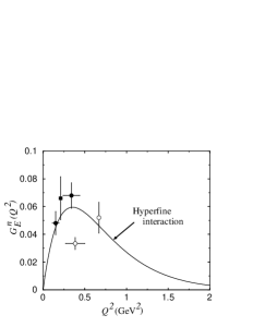
Figure 9: Electric neutron form factor in the hyperfine perturbed quark model with a harmonic oscillator potential.

In the harmonic oscillator model at leading order in $\alpha_{s}$, the hyperfine interaction gives rise to a neutron electric form factor [93]:

$$G_{E}^{n}(Q^{2}) = -{1\over 6}\left<\sum_{i}e_{i}r_{i}^{2}\right>_{n}Q^{2}\exp\left(-Q^{2}/6\alpha^{2}\right)\ ,$$ (91)

where $\alpha$ can be related to decay amplitudes and charge radii [92]. Taking the value $\alpha=0.243$ from the ratio of neutron to proton charge radii, the resulting form factor in Fig. 9 agress quite well with the available $G_{E}^{n}$ data. More accurate data, which will soon be available from Jefferson Lab and elsewhere over a range of $Q^{2}$ will allow more systematic comparison of the various mechanisms which contribute to SU(6) symmetry breaking.

4.3 Strange Quarks in the Nucleon

A complication in studying the light quark sea is the fact that non-perturbative features associated with $u$ and $d$ quarks are intrinsically correlated with the valence core of the proton, so that effects of $q\bar{q}$ pairs can be difficult to distinguish from those of antisymmetrization or residual interactions of quarks in the core. The strange sector, on the other hand, where antisymmetrization between sea and valence quarks plays no role, is therefore more likely to provide direct information about the non-perturbative origin of the nucleon sea [95].

Evidence for non-perturbative strangeness is currently being sought in a number of processes, ranging from semi-inclusive neutrino induced deep-inelastic scattering to parity violating electron–proton scattering. As for the $\bar{d}-\bar{u}$ asymmetry, perturbative QCD alone generates identical $s$ and $\overline{s}$ distributions, so that any asymmetry would have to be non-perturbative in origin.

Figure 10: Strange quark asymmetry in the proton arising from a kaon cloud of the nucleon. The shaded region indicates current experimental limits from the CCFR Collaboration [96].

In deep-inelastic scattering, the CCFR collaboration [96] analyzed charm production cross sections in $\nu$ and $\bar{\nu}$ reactions, which probe the $s$ and $\bar{s}$ distributions in the nucleon, respectively. The resulting difference $s-\bar{s}$, indicated in Fig. 10 by the shaded area, has been extracted from the $s/\bar{s}$ ratio and absolute values of $s+\bar{s}$ from global data parameterizations.

The curve in Fig. 10 corresponds to the chiral cloud model prediction for the asymmetry (in analogy with the pion cloud in Section 4.2), in which the strangeness in the nucleon is carried by kaons and hyperons, so that the $s$ and $\bar{s}$ quarks have quite different origins [77, 97]. Taking the $\Lambda$ hyperon as an illustration (the results generalize straightforwardly to other hyperons such as the $\Sigma$), the difference between the $s$ and $\bar{s}$ can be written [98]:

$$s(x)-\bar{s}(x) = \int_{x}^{1}{dy\over y}\left(f_{\Lambda K}(y)\ s^{\Lambda}(x/y)\ -f_{K\Lambda}(y)\ \bar{s}^{K}(x/y)\right)\ ,$$ (92)

where the $K$ distribution function $f_{K\Lambda}$ is the analog of the $\pi N$ splitting function in Eq.(79), and the corresponding $\Lambda$ distribution $f_{\Lambda K}(y)=f_{K\Lambda}(1-y)$.

In the IMF parameterization of the $KNY$ ($Y=\Lambda,\Sigma$) vertex function, because the $\bar{s}$ distribution in a kaon is much harder than the $s$ distribution in a hyperon, the resulting $s-\bar{s}$ difference is negative at large $x$, despite the kaon distribution in the nucleon being slightly softer than the hyperon distribution [98]. With a dipole cut-off mass of $\Lambda\sim 1$ GeV, the kaon probability in the nucleon is $\approx 3\%$. On the other hand, the exact shape and even sign of the $s-\bar{s}$ difference as a function of $x$ is quite sensitive to the shape of the $KNY$ vertex [98].

Overall, while the current experimental $s-\bar{s}$ difference is consistent with zero, it does also consistent with a small amount of non-perturbative strangeness, which would be generated from a kaon cloud around the nucleon [98]. Of course other, heavier strange mesons and hyperons can be added to the analysis, although in the context of chiral symmetry [99] the justification for inclusion of heavier pseudoscalar as well as vector mesons is less clear. The addition of the towers of heavier mesons and baryons has also been shown in a quark model [77] to lead to significant cancellations, leaving the net strangeness in the nucleon quite small.

Figure 11: Strange electromagnetic form factors of the proton compared with a kaon cloud prediction, with the magnetic ($M$), electric ($E$) and total contributions indicated. For the HAPPEX data [101], $r\approx 0.4$.

Within the same formalism as used to discuss strange quark distributions one can also calculate the strangeness form factors of the nucleon, which are being measured in parity-violating electron scattering experiments at MIT-Bates [100] and Jefferson Lab [101]. The HAPPEX Collaboration at Jefferson Lab [101] has recently measured the left-right asymmetry $A_{LR}$ in $\vec{e}p\rightarrow ep$ elastic scattering, which measures the $\gamma^{*}Z$ interference term:

$$A = {\sigma_{R}-\sigma_{L}\over\sigma_{R}+\sigma_{L}}\ =\ \left({-G_{F}\over\pi\alpha_{em}\sqrt{2}}\right){1\over\varepsilon\ G_{E}^{p2}+\tau\ G_{M}^{p2}}$$ (93)

$$\times\left(\varepsilon\ G_{E}^{p}\ G_{E}^{p(Z)}+\tau\ G_{M}^{p}\ G_{M}^{p(Z)}-{1\over 2}(1-4\sin^{2}\theta_{W})\ \varepsilon^{\prime}\ G_{M}^{p}\ G_{A}^{p(Z)}\right),$$

with $\varepsilon=\left(1+2(1+\tau)\tan^{2}(\theta/2)\right)^{-1}$, and $\varepsilon^{\prime}=\sqrt{\tau(1+\tau)(1-\varepsilon^{2})}$ (the $Q^{2}$ dependence in all form factors is implicit). Using isospin symmetry, one can relate the electric and magnetic form factors for photon and $Z$-boson exchange via:

$$G_{E,M}^{p(Z)} = {1\over 4}G_{E,M}^{(I=1)}-\sin^{2}\theta_{W}\ G_{E,M}^{p}-{1\over 4}G_{E,M}^{s}\ ,$$ (94)

where $G_{E,M}^{(I=1)}$ is the isovector form factor. At forward angles, the asymmetry is sensitive to a combination of strange electric and magnetic form factors shown in Fig. 11 for $Q^{2}=0.48$ GeV². With a soft $KNY$ form factor the contributions to both $G_{E}^{s}$ and $G_{M}^{s}$ are small and slightly positive [98], in agreement with the trend of the data. This result is consistent with the earlier experiment by the SAMPLE Collaboration at MIT-Bates [100], $G_{M}^{s}=+0.23\pm 0.44$ at $Q^{2}=0.1$ GeV² in a similar experiment but at backward angles.

Although the experimental results on non-perturbative strangeness in both structure functions and form factors are still consistent with zero, they are nevertheless compatible with a soft kaon cloud around the nucleon. Future data on $G_{E/M}^{s}$ from the HAPPEX-II and G0 experiments at Jefferson Lab with smaller error bars and over a large range of $Q^{2}$, as well as the remaining data on the proton and deuteron from SAMPLE, will hopefully provide conclusive evidence for the presence or otherwise of a tangible non-perturbative strange component in the nucleon.

4.4 Polarized Quarks

Most of the discussion thus far has dealt with the flavor dependence of quarks in the nucleon. On the other hand, there has been considerable interest over the past decade in how the spin of the nucleon is distributed amongst its constituents ^102-104. Spin degrees of freedom allow access to information about the structure and interactions of hadrons which would otherwise not be available through unpolarized processes. Indeed, experiments involving spin-polarized beams and targets have often yielded surprising results and presented severe challenges to existing theories.

A fundamental sum rule for the spin in the nucleon states that:

$${1\over 2} = J_{q}\ +\ J_{g}\ ,$$ (95)

where $J_{q}$ and $J_{g}$ are the total quark and gluon angular momenta, which can be decomposed into their helicity and orbital contributions:

$$J_{q} = {1\over 2}\Delta\Sigma\ +\ L_{q}\ ,$$ (96)

$$J_{g} = \Delta G\ +L_{g}\ .$$ (97)

In particular, $\Delta\Sigma$, which is defined as the forward matrix element of the axial current, $\Delta\Sigma=\langle N|\bar{\psi}\gamma_{3}\gamma_{5}\psi|N\rangle$, measures the total helicity of the nucleon carried by quarks, which for three flavors is:

$$\Delta\Sigma = \Delta u+\Delta d+\Delta s\ .$$ (98)

In non-relativistic quark models the spin of the nucleon is carried entirely by valence quarks, so that $\Delta\Sigma_{\rm NRQM}=1$.

The gluon helicity, $\Delta G$, can be measured in high-energy polarized proton–proton collisions, via charm production through quark–gluon fusion, or in production of jets with high transverse momentum [105]. The orbital contributions, $L_{q}$ and $L_{g}$, can in principle be extracted from measurements of off-forward parton distributions in DVCS, or deeply-virtual meson production experiments [39]. Currently there is little empirical information on the gluon polarization, and the angular momentum distributions are totally unknown. Note that each term in Eqs.(96) and (97) is renormalization scheme and scale dependent, and only the quark helicity can be defined in a gauge-invariant manner [39].

Experimentally, $\Delta\Sigma$ (which is also referred to as the singlet axial charge) can be determined from a combination of triplet and octet axial charges,

$$g_{3} = \Delta u-\Delta d\ =\ g_{A}\ ,$$ (99)

$$g_{8} = \Delta u+\Delta d\ -\Delta s\ ,$$ (100)

which are determined from $\beta$-decays of the nucleon and hyperons, and the spin-dependent $g_{1}$ structure function of the nucleon. In the $\overline{\rm MS}$ scheme, the lowest moment of the $g_{1}$ structure function (at lowest order in perturbative QCD) is given by [23, 104, 106]:

$$\int_{0}^{1}dxg_{1}^{p(n)}(x,Q^{2}) = \left[1-\left({\alpha_{s}\over\pi}\right)\right]\left(\pm{1\over 12}g_{3}\ +\ {1\over 36}g_{8}\ +\ {1\over 9}\Delta\Sigma\right),$$ (101)

where the $\pm$ refers to the proton or neutron.

The first spin structure function experiments at CERN [107] suggested a rather small value for $\Delta\Sigma$, in fact consistent with zero, which prompted the so-called ‘proton spin-crisis’. A decade of subsequent measurements of inclusive spin structure functions using proton, deuteron and ³He targets have [108] determined $\Delta\Sigma$ much more accurately, with the current world average value [104] (at a scale of $Q^{2}=10$ GeV² in the $\overline{\rm MS}$ scheme) being $\Delta\Sigma\approx 0.3$.

While the spin fractions carried by quarks in the nucleon require only the first moment of the inclusive spin-dependent structure functions, to determine the $x$ dependence of the polarized distributions requires independent linear combinations of $\Delta q$ which at present can only be obtained from semi-inclusive scattering. Generalizing Eq.(52) to the production of hadrons with a polarized beam and target, $\vec{e}\vec{N}\rightarrow e^{\prime}hX$, the difference between the number of hadrons produced at a given $x$, $z$ and $Q^{2}$ with electron and nucleon spins parallel and antiparallel is (at leading order) given by:

$$\Delta N^{h}\ \equiv\ N^{h}_{\uparrow\Uparrow-\downarrow\Uparrow}(x,z,Q^{2}) \sim \sum_{q}e_{q}^{2}\ \Delta q(x,Q^{2})\ \Delta D_{q}^{h}(z,Q^{2})\ ,$$ (102)

where the polarized fragmentation function $\Delta D_{q}^{h}$ gives the probability for a polarized quark $q$ to hadronize into a hadron $h$.

In analogy with the large-$x$ behavior of the unpolarized $u$ and $d$ distributions in Section 4.1, the $x\rightarrow 1$ limit of polarized quark distributions provides a sensitive test of various mechanisms of spin-flavor symmetry breaking. For SU(6) symmetry, the ratio of the polarized to unpolarized quark distributions is:

$${\Delta u\over u} = {2\over 3}\ ,\ \ \ \ \ {\Delta d\over d}\ =\ -{1\over 3}\ \ \ \ \ [{\rm SU(6)\ symmetry}]\ .$$ (103)

If the symmetry is broken through the suppression of the $S=1$ diquark contributions in the nucleon, then in the limit $x\rightarrow 1$:

$${\Delta u\over u} \longrightarrow 1\ ,\ \ \ \ \ {\Delta d\over d}\ \longrightarrow\ -{1\over 3}\ \ \ \ [S=0\ {\rm dominance}]\ .$$ (104)

The perturbative QCD prediction (where the dominant configurations of the proton wave function are those in which the spins of the interacting quark and proton are aligned) on the other hand, is:

$${\Delta u\over u} \longrightarrow 1\ ,\ \ \ \ \ {\Delta d\over d}\ \longrightarrow\ 1\ \ \ \ \ [S_{z}=0\ {\rm dominance}]\ .$$ (105)

Note that the predictions for the $\Delta d$ quark in particular are quite different in the perturbative and non-perturbative models, even differing by sign.

The spin-flavor distributions can be directly measured via polarization asymmetries for the difference between $\pi^{+}$ and $\pi^{-}$ production cross sections on the proton [109, 110]:

$$A_{p}^{\pi^{+}-\pi^{-}} = {\Delta N_{p}^{\pi^{+}}-\Delta N_{p}^{\pi^{-}}\over\Delta N_{p}^{\pi^{+}}+\Delta N_{p}^{\pi^{-}}}\ =\ {4\Delta u_{\rm val}-\Delta d_{\rm val}\over 4u_{\rm val}-d_{\rm val}}\ ,$$ (106)

where the dependence on fragmentation functions and sea quarks cancels. A combination of inclusive and semi-inclusive asymmetries using protons and deuterons at an energy upgraded Jefferson Lab will allow the spin-dependent $\Delta u$ and $\Delta d$ distributions to be determined up to $x\sim 0.8$ with good statistics [111], which should be able to discriminate between the various model scenarios in Eqs.(103)-(105).

At smaller $x$, similar combinations of asymmetries could also be able to measure the polarized antiquark distributions, $\Delta\bar{d}$ and $\Delta\bar{u}$. These are particularly interesting in view of the qualitatively different predictions in non-perturbative models. While chiral (pion) cloud models do not allow any polarization in the antiquark sea, the Pauli exclusion principle on the other hand predicts quite a large asymmetry, $(\Delta\bar{u}-\Delta\bar{d})/(\bar{d}-\bar{u})=5/3$, even bigger than in the unpolarized sea [26, 112]. Measurement of the polarized asymmetry in semi-inclusive scattering would then enable the relative sizes of the pion and Pauli blocking contributions to $\bar{d}-\bar{u}$ to be disentangled.

While data on the polarized quark distributions has slowly been accumulating from various experiments, and plans are under way to systematically measure the polarization of the gluons, until recently there has been very little discussion about the fraction of the nucleon spin residing in angular momentum [113]. This changed somewhat when it was demonstrated [39] that the orbital angular momentum contributions could be determined from off-forward parton distributions measured in deeply-virtual Compton scattering (see Section 3.4).

In particular, it was shown [39] that a sum rule can be derived relating moments of the OFPDs to the total angular momentum carried by quarks and gluons:

$$\int_{-1}^{1}dx\ x\Big{(}H(x,\xi,t)+E(x,\xi,t)\Big{)} = A(t)+B(t)\ ,$$ (107)

where $A$ and $B$ are form factors of the energy-momentum tensor in QCD [114]:

$$T^{\mu\nu}_{q} = {1\over 2}\left(\overline{\psi}\gamma^{\{\mu}i\overrightarrow{D^{\nu\}}}\psi+\overline{\psi}\gamma^{\{\mu}i\overleftarrow{D^{\nu\}}}\psi\right)\ ,$$ (108)

$$T^{\mu\nu}_{g} = {1\over 4}g^{\mu\nu}F^{2}-F^{\mu\alpha}F^{\nu}_{~{}\alpha}\ .$$ (109)

for quarks and gluons, respectively, where the braces $\{\cdots\}$ represent symmetrization of indices. The matrix elements of $T^{\mu\nu}$ can be expanded as [39]:

$$\langle P^{\prime}|T^{\mu\nu}|P\rangle = \overline{u}(P^{\prime})\Big{[}{1\over 2}A(t)\ \gamma^{\{\mu}(P+P^{\prime})^{\nu\}}\$$ (110)

$$+\ {1\over 4M}B(t)\ (P+P^{\prime})^{\{\mu}i\sigma^{\nu\}\alpha}(P^{\prime}-P)_{\alpha}+\cdots\Big{]}u(P)\ .$$

One can then show that the total angular momentum carried by quarks is given by:

$$J_{q} = {1\over 2}\Big{(}A(0)+B(0)\Big{)}\ .$$ (111)

Combining the extracted $J_{q}$ with $\Delta\Sigma$ measured in inclusive DIS, one can then determine the orbital angular momentum of the quarks in the nucleon. An analogous sum rule can also be written for the total gluon angular momentum, $J_{g}$, which can be obtained from OFPDs measured in deeply-virtual meson production. From this the gluon orbital angular momentum can be extracted once the gluon helicity $\Delta G$ is known.

The program to measure the off-forward parton distributions $H,E,\cdots$ in deeply-virtual Compton scattering and meson production experiments is difficult, requiring a large coverage of kinematics and knowledge of background such as the Bethe-Heitler process [115] for DVCS. The first steps along the road to mapping out these fundamental quantities are already being taken at Jefferson Lab and HERMES.

5 Conclusion

Thanks to recent advances in accelerator technology that have enabled precise data to be collected at the world’s particle accelerators, we have been able to probe the fascinating inner structure of the nucleon with unprecedented clarity. Though much has been learned from inclusive DIS experiments, future analyses of nucleon structure will focus more on semi-inclusive reactions, which will enable the spin and flavor composition of protons and neutrons to be resolved with greater precision. Furthermore, there is a growing appreciation of the need to understand the common underlying physics revealed through a range of observables, from elastic form factors to deep-inelastic structure functions.

Some of the most exciting recent developments have been in the study of the non-perturbative structure of the proton sea through asymmetries in sea quark distributions, which illustrate the relevance of chiral symmetry breaking in QCD even at high energies. Important breakthroughs in our understanding of the proton spin have opened the way to accessing for the first time information about the full helicity and orbital momentum distributions in the nucleon. In addition, perhaps longest overdue is the need to determine the valence quark distributions in the region of large Bjorken-$x$, which should settle the long-standing puzzle of the precise $x\rightarrow 1$ behavior of structure functions and shed light on the mechanisms of spin-flavor symmetry breaking in the nucleon.

To make the inroads necessary to achieve a deeper understanding of these issues will require full utilization of the high luminosities and machine duty factors at modern accelerator facilities such as Jefferson Lab. We can anticipate the new generations of experiments to reveal much more of the intriguing world of subnucleon dynamics.

References

References

- [1] H. Yukawa, Proc. Phys. Math. Soc. Japan 17, 48 (1935).
- [2] G.C. Wick, Nature 142, 993 (1938).
- [3] M. Gell-Mann, Phys. Lett. 8, 214 (1964); G. Zweig, CERN preprint 8419/TH 412 (1964).
- [4] O.W. Greenberg, Phys. Rev. Lett. 13, 598 (1964); M.Y. Han and Y. Nambu, Phys. Rev. 139, 1006 (1965).
- [5] W.K.H. Panofsky, in Proceedings of the 14th International Conference on High Energy Physics, Vienna, 1968 (CERN Scientific Information Service, Geneva); E.D. Bloom et al., Phys. Rev. Lett. 23, 930 (1969); J.I. Friedman and H.W. Kendall, Ann. Rev. Nucl. Part. Sci. 22, 203 (1972).
- [6] H. Fritzsch and M. Gell-Mann, in Proceedings of the 16th. International Conference on High Energy Physics, ed. J.P. Jackson and A. Roberts (National Accelerator Lab., Batavia, Illinois, 1972); H. Fritzsch, M. Gell-Mann and H. Leutwyler, Phys. Lett. B 47, 365 (1973); D.J. Gross and F. Wilczek, Phys. Rev. D 8, 3633 (1973).
- [7] N. Isgur, in Proceedings of the 26th International Conference on High Energy Physics (ICHEP 92), Dallas, Texas, August 1992.
- [8] A.J. Buras, Rev. Mod. Phys. 52, 199 (1980).
- [9] F.J. Yndurain, Quantum Chromodynamics (Springer-Verlag, Berlin, 1983).
- [10] T. Muta, Foundations of Quantum Chromodynamics (World Scientific, Singapore, 1987).
- [11] G. Sterman et al., Rev. Mod. Phys. 67, 157 (1995).
- [12] K.G. Wilson, Phys. Rev. D 10, 2445 (1974); D.G. Richards, these proceedings, nucl-th/0006020.
- [13] S. Weinberg, Physica (Amsterdam) 96 A, 327 (1979); J. Gasser and H. Leutwyler, Ann. Phys. 158, 142 (1984); B.R. Holstein, hep-ph/9911449, and these proceedings.
- [14] A.J.G. Hey and J.E. Mandula, Phys. Rev. D 5, 2610 (1972).
- [15] E. Leader and E. Predazzi, An Introduction to Gauge Theories and Modern Particle Physics (Cambridge Univ. Press, 1996).
- [16] I. Niculescu, private communication.
- [17] R. Hofstadter and R.W. McAllister, Phys. Rev. 98, 183 (1955); R.W. Mcallister and R. Hofstadter, Phys. Rev. 102, 851 (1956). R. Hofstadter et al., Phys. Rev. Lett. 5, 263 (1960).
- [18] G.P. Lepage and S.J. Brodsky, Phys. Rev. Lett. 43, 545 (1979); Phys. Rev. D 22, 2157 (1980).
- [19] R.P. Feynman, in Proceedings of the 3rd Topical Conference on High Energy Collisions of Hadrons, Stony Brook, NY, ed. C.N. Yang et al. (Gordon & Breach, New York, 1969); Phys. Rev. Lett. 23, 1415 (1969).
- [20] J.D. Bjorken and E.A. Paschos, Phys. Rev. 185, 1975 (1969).
- [21] K. Wilson, Phys. Rev. 179, 1499 (1969); R.A. Brandt and G. Preparata, Nucl. Phys. B 27, 541 (1971); O. Nachtmann, Nucl. Phys. B 63, 237 (1973).
- [22] R.L. Jaffe, Nucl. Phys. B 229, 205 (1983).
- [23] T. Weigl and W. Melnitchouk, Nucl. Phys. B 465, 267 (1996).
- [24] A. Le Yaouanc, L. Oliver, O. Pène and J.C. Reynard, Phys. Rev. D 9, 2636 (1974); R.L. Jaffe, Phys. Rev. D 11, 1953 (1975); N. Cabbibo and R. Petronzio, Nucl. Phys. B 137, 395 (1978); C.J. Benesh and G.A. Miller, Phys. Rev. D 36, 1344 (1987).
- [25] A.I. Signal and A.W. Thomas, Phys. Rev. D 40, 2832 (1989); A.W. Schreiber, A.W. Thomas and J.T. Londergan, Phys. Lett. B 237, 120 (1989).
- [26] A.W. Schreiber, A.I. Signal and A.W. Thomas, Phys. Rev. D 44, 2653 (1991).
- [27] R.L. Jaffe and G.G. Ross, Phys. Lett. 93 B, 313 (1980).
- [28] G. Parisi and R. Petronzio Phys. Lett. 62 B, 331 (1976).
- [29] H. Georgi and H.D. Politzer, Phys. Rev. D 9, 416 (1974).
- [30] D.J. Gross and F. Wilczek, Phys. Rev. D 9, 920 (1974).
- [31] Yu.L. Dokshitzer, Sov. Phys. JETP 46, 641 (1977); V.N. Gribov and L.N. Lipatov, Sov. J. Nucl. Phys. 15, 439 (1972); L.N. Lipatov, Sov. J. Nucl. Phys. 20, 181 (1974); G. Altarelli and G. Parisi, Nucl. Phys. B 126, 278 (1977).
- [32] H.L. Lai et al., Eur. Phys. J. C 12, 375 (2000).
- [33] A.D. Martin, R.G. Roberts, W.J. Stirling and R.S. Thorne, Eur. Phys. J. C 4, 463 (1998).
- [34] M. Gluck, E. Reya and A. Vogt, Eur. Phys. J. C 5, 461 (1998).
- [35] P.V. Landshoff and J.C. Polkinghorne, Nucl. Phys. B 33, 221 (1971); J. Ellis, Phys. Lett. B 35, 537 (1971); J.D. Stack, Phys. Rev. Lett. 28, 57 (1972); T. Sloan, G. Smadja and R. Voss, Phys. Rep. 162, 45 (1980); R. Renton and W.S.C. Williams, Ann. Rev. Nucl. Part. Sci. 31, 193 (1981).
- [36] W. Melnitchouk, in Proceedings of the Workshop on Physics with a High-Luminosity Polarized Electron-Ion Collider, IUCF, April 1999, hep-ph/9906488.
- [37] K. Ackerstaff, First Results from the HERMES Experiment using Unpolarized Targets, PhD thesis, Univ. Hamburg, 1996.
- [38] J.J. Aubert et al., Phys. Lett. B 110, 73 (1982); Nucl. Phys. B 213, 213 (1983).
- [39] X. Ji, Phys. Rev. Lett. 78, 610 (1997); J. Phys. G 24, 1181 (1998).
- [40] A.V. Radyushkin, Phys. Rev. D 56, 5524 (1997).
- [41] R.L. Jaffe and X. Ji, Phys. Rev. Lett. 67, 552 (1991); A.V. Manohar, Phys. Rev. Lett. 66, 289 (1991).
- [42] X. Ji, W. Melnitchouk and X. Song, Phys. Rev. D 56, 5511 (1997).
- [43] S. Kuhlmann et al., Phys. Lett. B 476, 291 (2000).
- [44] W. Melnitchouk and A.W. Thomas, Phys. Lett. B 377, 11 (1996).
- [45] F.E. Close, An Introduction to Quarks and Partons (Academic Press, 1979).
- [46] R.P. Feynman, Photon Hadron Interactions (Benjamin, Reading, Massachusetts, 1972).
- [47] F.E. Close, Phys. Lett. B 43, 422 (1973).
- [48] R. Carlitz, Phys. Lett. B 58, 345 (1975).
- [49] F.E. Close and A.W. Thomas, Phys. Lett. B 212, 227 (1988).
- [50] N. Isgur, Phys. Rev. D 59, 034013 (1999).
- [51] G.R. Farrar and D.R. Jackson, Phys. Rev. Lett. 35, 1416 (1975).
- [52] W. Melnitchouk, A.W. Schreiber and A.W. Thomas, Phys. Lett. B 335, 11 (1994); Phys. Rev. D 49, 1183 (1994).
- [53] W. Melnitchouk and J.C. Peng, Phys. Lett. B 400, 220 (1997).
- [54] W. Melnitchouk, M. Sargsian and M.I. Strikman, Z. Phys. A 359, 99 (1997).
- [55] P. Souder, in Proceedings of Workshop on CEBAF at Higher Energies, CEBAF, Newport News, 1994; R. Michaels, in Physics and Instrumentation with 6-12 GeV Beams, Jefferson Lab, Newport News, June 1998.
- [56] H1 Collaboration, C. Adloff et al., DESY-99-107, hep-ex/9908059; ZEUS Collaboration, J. Breitweg et al., DESY-99-059, hep-ex/9907010.
- [57] G.G. Petratos et al., in Proceedings of Workshop on Experiments with Tritium at JLab, Jefferson Lab, Newport News, Virginia, September 1999; I.R. Afnan et al., nucl-th/0006003.
- [58] W. Melnitchouk, J. Speth and A.W. Thomas, Phys. Lett. B 435, 420 (1998).
- [59] E.D. Bloom and F.J. Gilman, Phys. Rev. Lett. 16, 1140 (1970).
- [60] I. Niculescu, Ph.D. thesis, Hampton University, 1999; C. Keppel, talk presented at 7th International Workshop on Deep Inelastic Scattering and QCD (DIS 99), Zeuthen, Germany, Apr. 1999.
- [61] S.D. Drell and T.-M. Yan, Phys. Rev. Lett. 24, 181 (1970).
- [62] G.B. West, Phys. Rev. Lett. 24, 1206 (1970).
- [63] W. Melnitchouk, Phys. Rev. Lett. 86, 35 (2001).
- [64] A. De Rújula, H. Georgi and H.D. Politzer, Ann. Phys. 103, 315 (1975).
- [65] N. Isgur, S. Jeschonnek, W. Melnitchouk and J.W. Van Orden, Phys. Rev. D 64, 054005 (2001).
- [66] C.E. Carlson and N.C. Mukhopadhyay, Phys. Rev. D 58, 094029 (1998); Phys. Rev. D 41, 2343 (1989).
- [67] P. Mergell, U.-G. Meißner and D. Drechsel, Nucl. Phys. A 596, 367 (1996).
- [68] M.K. Jones et al., Phys. Rev. Lett. 84, 1398 (2000).
- [69] A. Watson, Science 283, 472 (1999).
- [70] P. Amaudraz et al., Phys. Rev. Lett. 66, 2712 (1991).
- [71] A. Baldit et al., Phys. Lett. B 332, 244 (1994).
- [72] E.A. Hawker et al., Phys. Rev. Lett. 80, 3715 (1998).
- [73] W. Melnitchouk and A.W. Thomas, Phys. Rev. D 47, 3783 (1993).
- [74] A.W. Thomas and W. Melnitchouk, Nucl. Phys. A 631, 296 (1998).
- [75] A.W. Thomas, Phys. Lett. B 126, 97 (1983).
- [76] S. Théberge, G.A. Miller and A.W. Thomas, Phys. Rev. D 22, 2838 (1980); A.W. Thomas, Adv. Nucl. Phys. 13, 1 (1984); D.H. Lu, A.W. Thomas and A.G. Williams, Phys. Rev. C 57, 2628 (1998).
- [77] P. Geiger and N. Isgur, Phys. Rev. D 55, 299 (1997).
- [78] S. Weinberg, Phys. Rev. 150, 1313 (1966); S.D. Drell, D.J. Levy, and T.M. Yan, Phys. Rev. D 1, 1035 (1970).
- [79] J. Speth and A.W. Thomas, Adv. Nucl. Phys. 24, 83 (1998).
- [80] J.D. Sullivan, Phys. Rev. D 5, 1732 (1972).
- [81] V.R. Zoller, Z. Phys. C 54, 425 (1992); Z. Phys. C 60, 141 (1993).
- [82] W. Melnitchouk and A.W. Thomas, Phys. Rev. D 47, 3794 (1993).
- [83] W. Melnitchouk and A.W. Thomas, Phys. Rev. D 47, 3794 (1993); H. Holtmann, A. Szczurek and J. Speth, Nucl. Phys. A 596, 631 (1996).
- [84] T. Kitagaki et al., Phys. Rev. D 42, 1331 (1990).
- [85] W. Melnitchouk, J. Speth and A.W. Thomas, Phys. Rev. D 59, 014033 (1999).
- [86] F.M. Steffens and A.W. Thomas, Phys. Rev. C 55, 900 (1997).
- [87] R.D. Field and R.P. Feynman, Phys. Rev. D 15, 2590 (1977).
- [88] J. Levelt, P.J. Mulders and A.W. Schreiber, Phys. Lett. B 263, 498 (1991).
- [89] K. Ackerstaff et al., Phys. Rev. Lett. 81, 5519 (1998).
- [90] W. Melnitchouk, in Proceedings of the Workshop on Exclusive & Semi-Exclusive Processes at High Momentum Transfer, Jefferson Lab, June 1999, hep-ph/9909463.
- [91] S. Platchkov et al., Nucl. Phys. A 510, 740 (1990); P. Stoler, Phys. Rep. 226, 103 (1993).
- [92] N. Isgur, G. Karl and R. Koniuk, Phys. Rev. Lett. 41, 1269 (1978).
- [93] N. Isgur, G. Karl and D.W.L. Sprung, Phys. Rev. D 23, 163 (1981).
- [94] N. Isgur, Phys. Rev. Lett. 83, 272 (1999).
- [95] X. Ji and J. Tang, Phys. Lett. B 362, 182 (1995).
- [96] A.O. Bazarko et al., Z. Phys. C 65, 189 (1995).
- [97] A.I. Signal and A.W. Thomas, Phys. Lett. B 191, 206 (1987).
- [98] W. Melnitchouk and M. Malheiro, Phys. Rev. C 55, 431 (1997); Phys. Lett. B 451, 224 (1999); Phys. Rev. C 56, 2373 (1997).
- [99] A.W. Thomas, W. Melnitchouk and F.M. Steffens, Phys. Rev. Lett. 85, 2892 (2000).
- [100] B. Mueller et al., Phys. Rev. Lett. 78, 3824 (1997).
- [101] K.A. Aniol et al., Phys. Rev. Lett. 82, 1096 (1999).
- [102] F.E. Close and R.G. Roberts, Phys. Lett. B 316, 165 (1993).
- [103] S.D. Bass and A.W. Thomas, Prog. Part. Nucl. Phys. 33, 449 (1994). S.D. Bass, Eur. Phys. J. A 5, 17 (1999).
- [104] B. Lampe and E. Reya, hep-ph/9810270.
- [105] G.K. Mallot, J. Phys. G 25, 1539 (1999).
- [106] X. Ji and P. Unrau, Phys. Lett. B 333, 228 (1994); X. Ji and W. Melnitchouk, Phys. Rev. D 56, 1 (1997).
- [107] J. Ashman et al., Phys. Lett. B 206, 364 (1988).
- [108] K. Abe et al., Phys. Rev. Lett. 79, 26 (1997); B. Adeva et al., Phys. Rev. D 58, 112001 (1998); K. Abe et al., ibid D 58 112003 (1998).
- [109] L.L. Frankfurt, M.I. Strikman, L. Mankiewicz, A. Schafer, E Rondio, A. Sandacz and V. Papavassiliou, Phys. Lett. B 230, 141 (1989).
- [110] K. Ackerstaff, Phys. Lett. B 464, 123 (1999).
- [111] T.A. Forest, private communication.
- [112] B. Dressler, K. Goeke, M.V. Polyakov and C. Weiss, Eur. Phys. J. C 14, 147 (2000); M. Glück and E. Reya, hep-ph/0002182; R.S. Bhalerao, hep-ph/0003075.
- [113] L. Sehgal, Phys. Rev. D 10, 1663 (1974); X. Ji, J. Tang and P. Hoodbhoy, Phys. Rev. Lett. 76, 740 (1996); S.V. Bashinsky and R.L. Jaffe, Nucl. Phys. B 536, 303 (1998); N. Mathur, S.J. Dong, K.F. Liu, L. Mankiewicz and N.C. Mukhopadhyay, hep-ph/9912289.
- [114] R.L. Jaffe and A. Manohar, Nucl. Phys. B 337, 509 (1990).
- [115] M. Vanderhaeghen, P.A.M. Guichon and M. Guidal, Phys. Rev. Lett. 80, 5064 (1998); Phys. Rev. D 60, 094017 (1999).